THE SUMMERTIME ARCTIC ATMOSPHERERussian drifting North Pole stations were also made available (e.g., Kahl et al. 1999). The atmospheric program during the summer of 2001 [Arctic Ocean

1305SEPTEMBER 2004AMERICAN METEOROLOGICAL SOCIETY |

I n recent years, scientists and scientific organiza-tions have increasingly stressed the significance ofthe Arctic in the global climate system. The past

decade has seen changes in near-surface air tempera-ture, ice extent, and upper-ocean stratification(Houghton et al. 2001), suggesting that anthropogenicclimate change has begun to affect the Arctic. Serreze

et al. (2000) discuss significant temperature increasesover the northern Eurasian and American landmassesof > 0.5∞C per decade, while Rigor et al. (2000) findtrends in winter temperatures of ~ +1∞C per decadeon the Eurasian side of the Arctic. Generally, thesetrends agree with the trends in the Arctic Oscillation(Thompson and Wallace 1998). Morison et al. (2000)discuss the inflow of warm and saline Atlantic waterthat recently has penetrated deeper into the Arctic,altering upper-ocean stability. Chapman and Walsh(1993) show a downward long-term trend in sea iceextent for 1961–90. Parkinson et al. (1999) show thatArctic sea ice extent has been decreasing by ~ 3% perdecade, using microwave data through 1996, whileComiso (2002) shows that the perennial sea ice extentis decreasing by > 9% per decade.

The Arctic is often assumed to have a large climatesensitivity, and anthropogenic climate change is pro-jected to be the largest in the Arctic (e.g., Houghtonet al. 2001). Arctic warming is ~ 2.5 times the globalaverage in the Coupled Model IntercomparisonProject (CMIP; Meehl et al. 2000) simulations(Räisänen 2001). However, the global models used forthese projections have problems reproducing even the

THE SUMMERTIME ARCTICATMOSPHERE

Meteorological Measurements during theMeteorological Measurements during theMeteorological Measurements during theMeteorological Measurements during theMeteorological Measurements during the Arctic Ocean Experiment 2001 Arctic Ocean Experiment 2001 Arctic Ocean Experiment 2001 Arctic Ocean Experiment 2001 Arctic Ocean Experiment 2001

BY MICHAEL TJERNSTRÖM, CAROLINE LECK, P. OLA G. PERSSON, MICHAEL L. JENSEN,STEVEN P. ONCLEY, AND ADMIR TARGINO

A summer expedition with the Swedish icebreaker Oden found a moist, cloudy, but

well-mixed Arctic boundary layer, with a persistent capping inversion, many shallow

mesoscale fronts, and features generally unique to polar conditions.

AFFILIATIONS: TJERNSTRÖM, LECK, AND TARGINO—StockholmUniversity, Stockholm, Sweden; PERSSON—National Oceanic andAtmospheric Administration/Environmental Technology Laboratory,and Cooperative Institute for Research in Environmental Studies,Boulder, Colorado; JENSEN—Cooperative Institute for Research inEnvironmental Studies, Boulder, Colorado; ONCLEY—NationalCenter for Atmospheric Research, Boulder, ColoradoA supplement to this article is available online (DOI:10.1175/BAMS-84-9-Tjernstrom)CORRESPONDING AUTHOR: Dr. Michael Tjernström, ArrheniusLaboratory, Department of Meteorology, Stockholm University,Stockholm S-106 91, SwedenE-mail: [email protected]:10.1175/BAMS-85-9-1305

In final form 12 April 2004”2004 American Meteorological Society

1306 SEPTEMBER 2004|

current Arctic climate. They are generally too warmand have systematic biases in the surface pressurefields, with surface radiative fluxes varying widelybetween models (Walsh et al. 2002). Consequently,the intermodel spread in CMIP climate-warming sce-narios is larger in the Arctic than elsewhere (Räisänen2001). The observed recent warming also appears tohave occurred mostly over the northern Eurasiancontinent, rather than over the central Arctic, as hadbeen suggested by many climate models (Serreze et al.2000).

The difficulties in simulating the Arctic climaterelate directly to an insufficient understanding of sev-eral strong feedback processes. The large climate sen-sitivity in models is due largely to the strongly posi-tive ice–albedo feedback: warming reduces the ice/snow cover, thereby reducing the surface albedo, thus,enhancing the warming. How climate models handlesea ice and snow, and the energy exchange at the sur-face is, therefore, critical. Battisti et al. (1997) showedthat a lack of physical detail in describing ice processesinhibits a realistic representation of natural variabil-ity in the Arctic climate. It also causes significant er-rors in global weather forecast models (Beesley et al.2000).

The ice/snow cover also has a pronounced effecton the turbulent surface fluxes. During winter, snow-covered ice insulates the atmosphere from the highheat capacity of the ocean. Combined with longwaveradiative cooling and the absence of solar forcing dur-ing the Arctic winter, this gives rise to persistentstable stratification in the Arctic boundary layer(ABL) about 75% of the time (Persson et al. 2002).Turbulence in very stable conditions is poorly under-stood (Mahrt 1998; Grachev et al. 2004). Duringsummer, melting ice and snow regulates the low-leveltemperature; additional energy input enhances melt-ing rather than heating the surface, while energy lossresults in freezing, rather than a cooling. When thisunique surface interacts with local boundary layerprocesses, it gives rise to a vertical structure foundonly in the Arctic.

Long periods of stable ABL conditions are inter-spersed with shorter periods with near-neutral con-ditions. This is forced by longwave radiation (Perssonet al. 2002) and directly related to boundary layerclouds, which are a known problem in models. Liquidwater droplets are present in a sizeable fraction evenat very low temperatures (Beesley et al. 2000; Intrieriet al. 2002b), and unusual vertical structures with lay-ering and decoupling from the surface are describedby Curry et al. (2000). Clouds play an important rolefor the surface radiative fluxes, determining the net

longwave radiation and regulating incoming solarradiation in summer. Over the Arctic pack ice, incontrast to midlatitude oceans, clouds often lead tosurface warming (Intrieri et al. 2002a). Curry (1986)discusses the connection of cloud effects to aerosolparticles and cloud microphysics. During summer,the influence of anthropogenic aerosol sources is lim-ited in the Arctic due to the typical large-scale circu-lations, and by efficient scavenging (Leck et al. 1996).The lack of aerosol particles, vital to the formation ofcloud condensation nuclei (CCN), regulates the ra-diative characteristics of the clouds, providing pos-sible complications to the ice–albedo feedback. If in-creased open water from enhanced melting alsoresults in an increase in the concentration of aerosolsfrom local biogenic sources, this may increase thereflectivity and change the lifetime of Arctic stratusclouds. This would constitute a negative feedback toclimate change.

Many of these factors are specific to the Arctic. Theice cover is also a reason for a relative lack of in situobservations, while producing a difficult and hostileenvironment for observational studies. Moreover,because the ice drifts, fixed permanent sites forlong-term measurements cannot be established.Consequently, the ensemble of observations formingthe empirical basis for the development of reliableparameterizations may be inadequate. This may beone reason for the difficulties in modeling the Arcticclimate, and the only realistic way to rectify this is toobtain detailed observations of climate-related pro-cesses in the Arctic. Detailed observations of theArctic surface layer and the energy balance at the sur-face, as well as vertical troposphere structure, areavailable from the Surface Heat Budget of the ArcticOcean (SHEBA; Uttal et al. 2002; Perovich et al. 1999)and, during a shorter period, the First InternationalSatellite Cloud Climatology Project (ISCCP) RegionalExperiment (FIRE) Arctic Clouds Experiment (Curryet al. 2000) complemented SHEBA with detailed air-borne measurements. Recently, observations made onRussian drifting North Pole stations were also madeavailable (e.g., Kahl et al. 1999).

The atmospheric program during the summer of2001 [Arctic Ocean Experiment (AOE) 2001; Lecket al. 2004] on the Swedish icebreaker Oden was thethird in a series of similar expeditions. The previoustwo expeditions in 1991 [International AOE (IAOE)-91; Leck et al. 1996] and 1996 (AOE-96; Leck et al.2001a) were focused on studying atmospheric chem-istry and aerosol chemistry/physics. We designedAOE-2001 to improve upon the previous observa-tional work by adding an enhanced meteorological


component, a better vertical profiling capability forexamining atmospheric chemistry and aerosols, anda marine biology component to investigate processesin open leads and ice. We attempted to characterizea column from a few hundred meters into the ocean,through the ice–ocean interface, up to a few kilome-ters into the atmosphere. AOE-2001 was an interdis-ciplinary experiment with three subprograms: marinebiology, atmospheric chemistry and aerosol chemis-try/physics, and meteorology (more informationavailable online at www.lu.se/eriksw/AOE-2001.html). Although this experiment was significantlyshorter than SHEBA, AOE-2001 had a stronger fo-cus on boundary layer structure. In addition, it wascarried out in the Atlantic sector of the Arctic, whichhas received comparatively less attention—at least forthe atmosphere—and was significantly farther north.Moreover, SHEBA almost entirely lacked the atmo-spheric chemistry and aerosol components present inAOE-2001.

The results from previous expeditions on Odenshowed that in addition to the strong and well-definedbiogenic source of dimethylsulfides (DMS; an impor-tant aerosol precursor; Leck and Persson 1996) in themarginal ice zone (MIZ), a previously unknown lo-cal source of aerosols in the pack ice seems to bepresent. It was speculated that this local source wasalso biogenic, located in open leads (Leck and Bigg1999; Bigg and Leck 2001; Leck et al. 2001b). Also,temporal variability of concentrations of aerosol andgases (e.g., DMS and NH3) were unexpectedly large,with time scales from minutes to hours. Order-of-magnitude changes withina day were not uncommon(Bigg et al. 1996, 2001).AOE-2001 was conceivedto better address these is-sues. This paper presentsthe AOE-2001 field pro-gram, focusing on the me-teorological measurements.There are three main pur-poses for the meteorologysubprogram:

1) to study and determinelikely causes for thepreviously observedtemporal variability ingases and aerosols;

2) to study boundary layermixing processes of im-portance for the energy

balance at the surface, and for bringing newlyformed particles into the ABL from the surface orbringing long-range-transported aerosol precur-sors down from the free troposphere; and

3) to collect boundary layer meteorology data thatwill enhance the understanding of the summer-time ABL dynamics and, thus, help to improvemodel formulations.

THE EXPEDITION. Oden (Fig. 1) is a diesel-powered, 108-m-long, 24,500-hp icebreaker, built inSweden in 1988 to assist in commercial shipping.Oden is particularly effective in the Arctic, capable ofbreaking 2-m-thick ice continuously at a speed of 3 kt,and was the first non-nuclear-powered icebreaker toreach the North Pole in July 1991. During the presentexpedition, the atmospheric program shared Odenwith other scientific programs: biogeochemistry,oceanography, and seismology. The expedition seg-ments had different scientific priorities that deter-mined the cruise plan and onboard activity. Parts ofthe atmospheric measurements were conducted con-tinuously; a 3-week ice drift (2–21 August 2001) wasthe main target period for the atmospheric program.

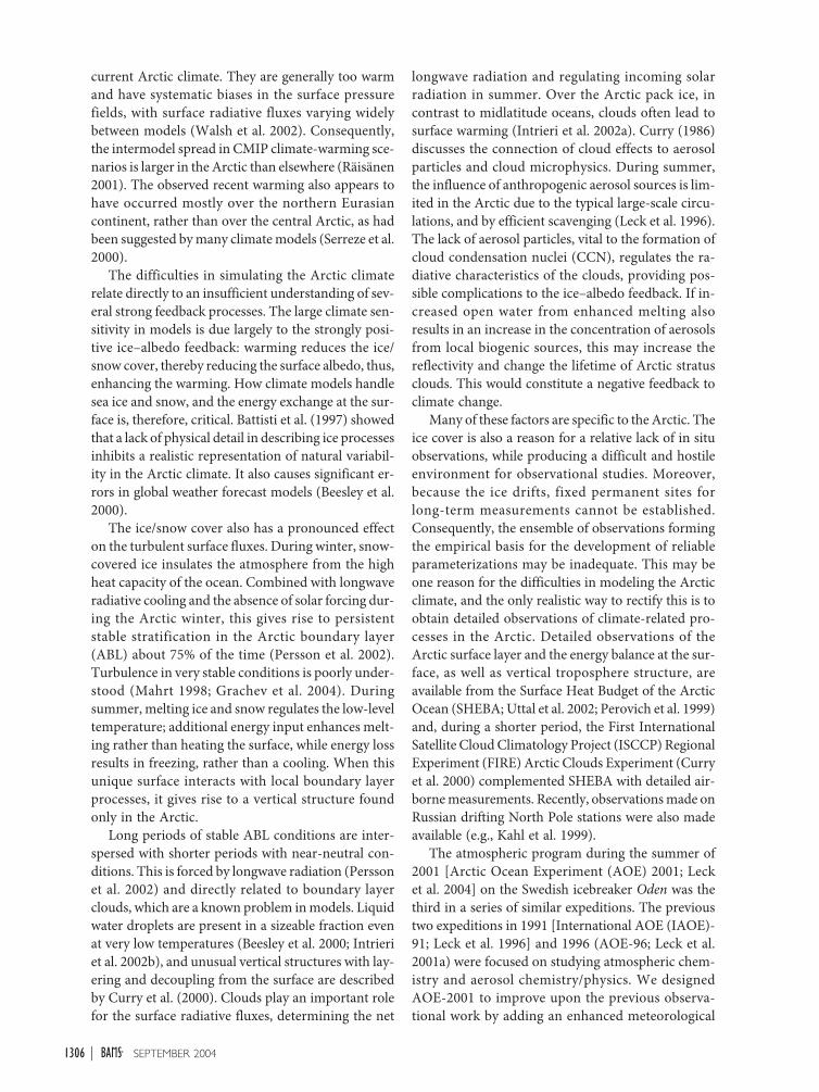
The track of the expedition is shown in Fig. 2. Theexpedition departed Gothenburg, Sweden, on 29 June2001, and the first research station was set up south-east of Svalbard on 5 July; two stations were estab-lished in this area. The expedition continued with twomore MIZ stations (9–10 and 11–12 July) and afterestablishing one more southerly research station inopen water northwest of Svalbard (15–16 July), Oden

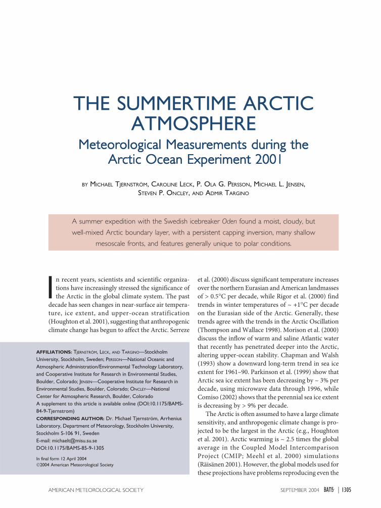
FIG. 1. Picture of the icebreaker Oden at the ice camp. The blue containerscarried research equipment or housed various laboratories. The tetheredballoon is visible at the stern.


headed into the pack ice on 17 July and traversed theGakkel ridge and Amundsen basin to the Lomonosovridge. Three more atmospheric research stations wereestablished (on 19, 22, and 27 July) before reachingthe North Pole on 31 July. During all of the shorterstation periods, many of the biology and atmosphericchemistry/aerosol subprograms were active; however,the meteorology subprogram was mostly limited toremote sensing instruments on board, rawinsound-ings, and the Oden weather station, due to insufficienttime to deploy the appropriate instruments on the ice,although the tethered sounding system and an Inte-grated Surface Flux Facility (ISFF)station was temporarily deployed afew times.

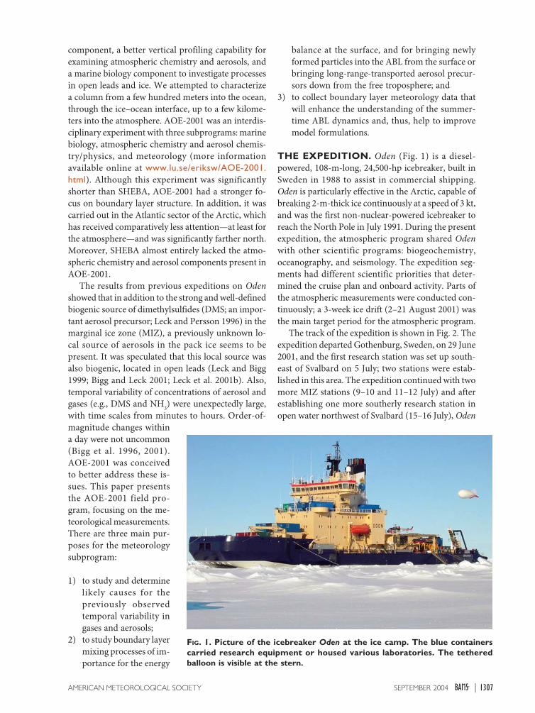
On 2 August Oden was moored toa relatively flat ~ 1.5 km × 3 km icefloe at ~ 89∞N, 1∞W (Fig. 3). Ice

thickness varied from ~ 1.5 to greater than 8 m, withthe latter at the site of the ice camp, presumably dueto subsurface ridging. The ice surface was coveredwith melt ponds of various sizes (see Fig. 3). Someponds eventually froze and became snow covered.Although August is at the end of the melt season, theice was stable for the duration of the experiment andthe ice drift continued with Oden attached to the sameice floe until 21 August. During this 3-week period,we drifted about 150 km in a generally southwesterlydirection (see insert to Fig. 2).

METEOROLOGICAL MEASUREMENTS. Theobjectives of the meteorological measurements calledfor both a continuous monitoring of the vertical struc-ture of the lower troposphere at a high temporal reso-lution and detailed ABL process studies. Althoughvertical structure was a main focus, we also wantedinformation on the horizontal structure and propa-gation of mesoscale systems. The measurement sys-tems that were deployed reflected all these needs.

A suite of remote sensing instruments was de-ployed on Oden, some later on the ice, to provide acontinuous record of vertical profiles of wind speedand direction, temperature, and clouds through thelower troposphere. Atmospheric moisture profileswere provided by the regularly released rawinsound-ings. Detailed studies of ABL turbulence and mixingrequire an undisturbed environment. Oden affectsmeasurements by disturbing airflow and from thenoise generated by its fans and hydraulics; the ice driftwas devised to alleviate these problems. Neighboringice floes were also utilized for some measurements.

FIG. 2. Plot of Oden’s track during AOE-2001, giving datesand locations for the atmospheric research stations.The insert shows the track while drifting with a largeice floe for the main 3-week atmospheric campaign.

FIG. 3. Aerial photograph of the ice floeused for the 3-week main atmosphericcampaign taken from the helicopter(15 Aug). The harbor (indicated by redarrow) set up by Oden to be able toshift mooring positions to face upwindis visible in the upper edge of the icefloe. Most of the atmospheric programwas carried out on the top-left quad-rant of the ice floe. The insert photo-graph shows the surface conditionsnear the mast and the sodar/tethersites on 8 Aug. Note the amount ofmelt ponds early during the ice drift.


A complete description of instrumentation can befound in an online supplement (Tjernström et al.2004), so only a summary is provided here as follows:

• Standard measurements: A weather station onOden’s top deck, ~ 30 m above the ocean surface,provided atmospheric variables and navigationalinformation continuously throughout the expedi-tion. Rawinsoundes were released from Oden’shelipad every 6 h during the ice drift and all shorterresearch stations.

• Remote sensing: A 915-MHz wind profiler, a scan-ning 5-mm radiometer for temperature profiles,and an S-band cloud and precipitation radar weredeployed on board. Two sodar systems were de-ployed on the ice.

• Tethered soundings: The Cooperative Institute forResearch in Environmental Sciences (CIRES)Tethered Lifting System (TLS) was operated on theice. Three payloads, for basic meteorology, 3D tur-bulence, and aerosols, were flown in various com-binations.

• The main mast: An 18-m meteorological telescop-ing mast about 300 m from Oden was equippedwith wind and temperature profile and turbulenceinstruments. The measurements also includedwind direction, absolute temperature, relative hu-midity, and a temperature profile into the ice, aswell as radiation and atmospheric pressure at thesurface.

• An array of microbarographs, for the detection ofgravity waves, was operated at the ice camp withthree sensors in a roughly equilateral triangularpattern ~ 200 m on each side, with a reference sen-sor in the center.

• Two ISFF stations were deployed on nearby icefloes ~ 8 km away from Oden to assess horizontalhomogeneity. These stations, forming a roughlyequilateral triangle with the main meteorologicalmast, made both turbulence and standard meteo-rological measurements.

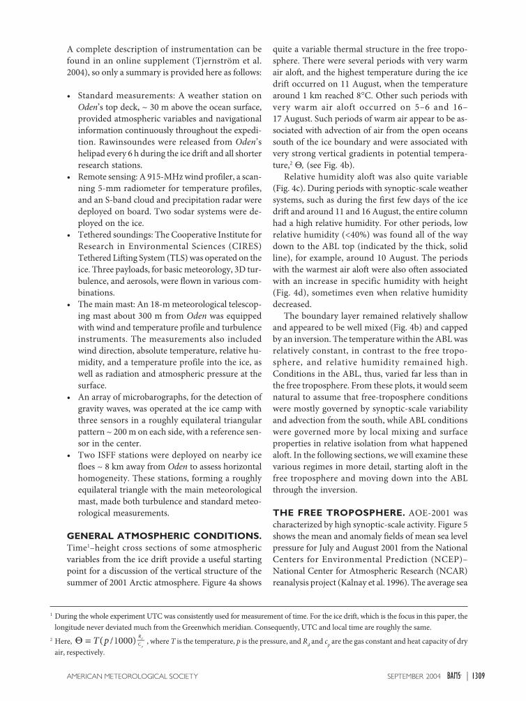
GENERAL ATMOSPHERIC CONDITIONS.Time1–height cross sections of some atmosphericvariables from the ice drift provide a useful startingpoint for a discussion of the vertical structure of thesummer of 2001 Arctic atmosphere. Figure 4a shows

quite a variable thermal structure in the free tropo-sphere. There were several periods with very warmair aloft, and the highest temperature during the icedrift occurred on 11 August, when the temperaturearound 1 km reached 8∞C. Other such periods withvery warm air aloft occurred on 5–6 and 16–17 August. Such periods of warm air appear to be as-sociated with advection of air from the open oceanssouth of the ice boundary and were associated withvery strong vertical gradients in potential tempera-ture,2 Q, (see Fig. 4b).

Relative humidity aloft was also quite variable(Fig. 4c). During periods with synoptic-scale weathersystems, such as during the first few days of the icedrift and around 11 and 16 August, the entire columnhad a high relative humidity. For other periods, lowrelative humidity (<40%) was found all of the waydown to the ABL top (indicated by the thick, solidline), for example, around 10 August. The periodswith the warmest air aloft were also often associatedwith an increase in specific humidity with height(Fig. 4d), sometimes even when relative humiditydecreased.

The boundary layer remained relatively shallowand appeared to be well mixed (Fig. 4b) and cappedby an inversion. The temperature within the ABL wasrelatively constant, in contrast to the free tropo-sphere, and relative humidity remained high.Conditions in the ABL, thus, varied far less than inthe free troposphere. From these plots, it would seemnatural to assume that free-troposphere conditionswere mostly governed by synoptic-scale variabilityand advection from the south, while ABL conditionswere governed more by local mixing and surfaceproperties in relative isolation from what happenedaloft. In the following sections, we will examine thesevarious regimes in more detail, starting aloft in thefree troposphere and moving down into the ABLthrough the inversion.

THE FREE TROPOSPHERE. AOE-2001 wascharacterized by high synoptic-scale activity. Figure 5shows the mean and anomaly fields of mean sea levelpressure for July and August 2001 from the NationalCenters for Environmental Prediction (NCEP)–National Center for Atmospheric Research (NCAR)reanalysis project (Kalnay et al. 1996). The average sea

1 During the whole experiment UTC was consistently used for measurement of time. For the ice drift, which is the focus in this paper, thelongitude never deviated much from the Greenwhich meridian. Consequently, UTC and local time are roughly the same.

2 Here, , where T is the temperature, p is the pressure, and Rd and cp are the gas constant and heat capacity of dryair, respectively.


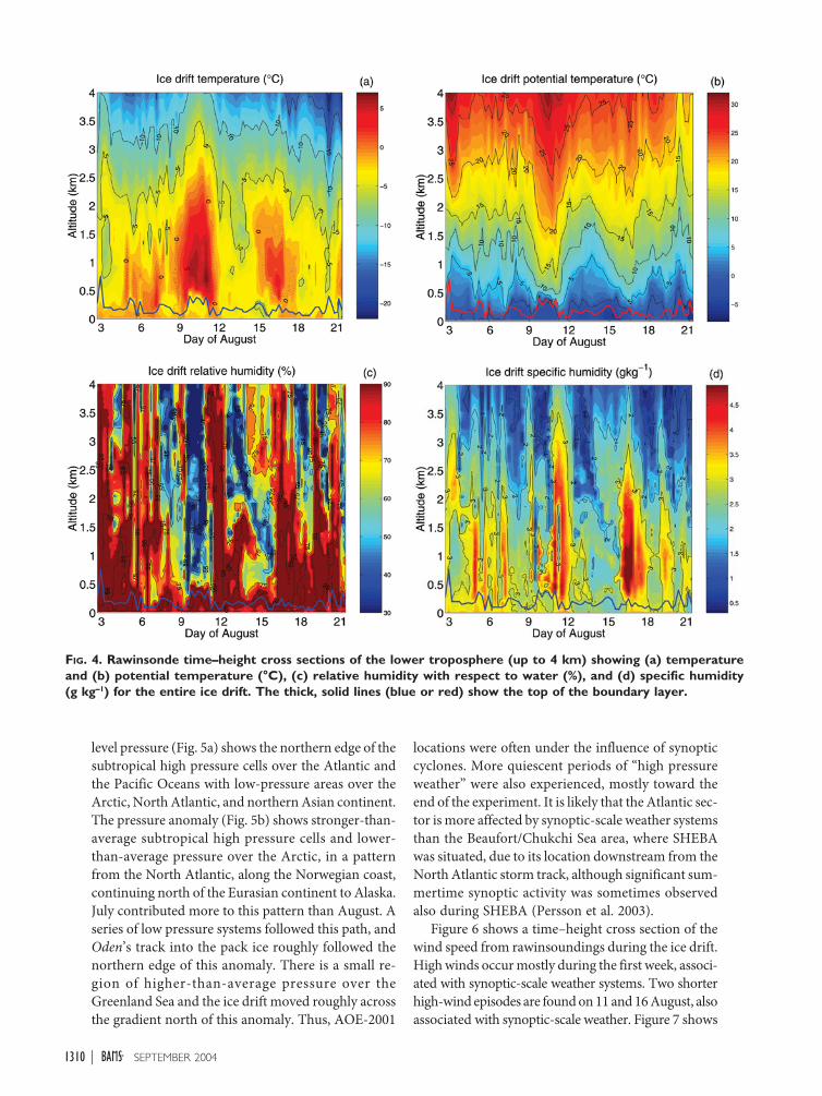
level pressure (Fig. 5a) shows the northern edge of thesubtropical high pressure cells over the Atlantic andthe Pacific Oceans with low-pressure areas over theArctic, North Atlantic, and northern Asian continent.The pressure anomaly (Fig. 5b) shows stronger-than-average subtropical high pressure cells and lower-than-average pressure over the Arctic, in a patternfrom the North Atlantic, along the Norwegian coast,continuing north of the Eurasian continent to Alaska.July contributed more to this pattern than August. Aseries of low pressure systems followed this path, andOden’s track into the pack ice roughly followed thenorthern edge of this anomaly. There is a small re-gion of higher-than-average pressure over theGreenland Sea and the ice drift moved roughly acrossthe gradient north of this anomaly. Thus, AOE-2001

locations were often under the influence of synopticcyclones. More quiescent periods of “high pressureweather” were also experienced, mostly toward theend of the experiment. It is likely that the Atlantic sec-tor is more affected by synoptic-scale weather systemsthan the Beaufort/Chukchi Sea area, where SHEBAwas situated, due to its location downstream from theNorth Atlantic storm track, although significant sum-mertime synoptic activity was sometimes observedalso during SHEBA (Persson et al. 2003).

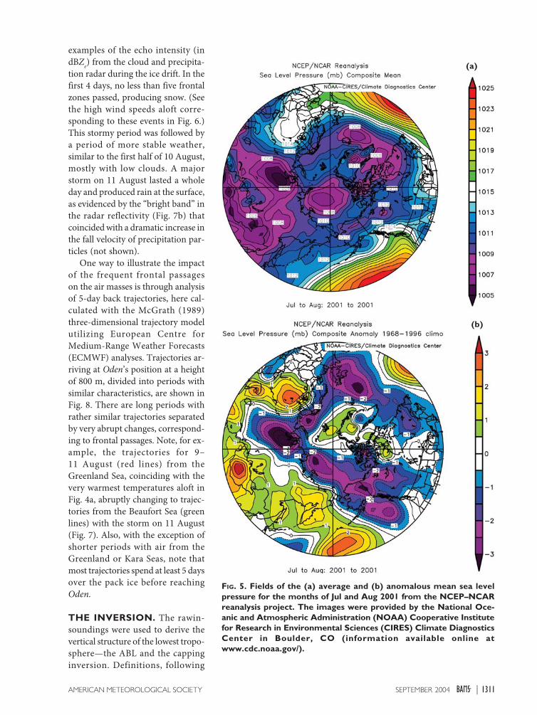
Figure 6 shows a time–height cross section of thewind speed from rawinsoundings during the ice drift.High winds occur mostly during the first week, associ-ated with synoptic-scale weather systems. Two shorterhigh-wind episodes are found on 11 and 16 August, alsoassociated with synoptic-scale weather. Figure 7 shows

FIG. 4. Rawinsonde time–height cross sections of the lower troposphere (up to 4 km) showing (a) temperatureand (b) potential temperature (°C), (c) relative humidity with respect to water (%), and (d) specific humidity(g kg-----1) for the entire ice drift. The thick, solid lines (blue or red) show the top of the boundary layer.


examples of the echo intensity (indBZe) from the cloud and precipita-tion radar during the ice drift. In thefirst 4 days, no less than five frontalzones passed, producing snow. (Seethe high wind speeds aloft corre-sponding to these events in Fig. 6.)This stormy period was followed bya period of more stable weather,similar to the first half of 10 August,mostly with low clouds. A majorstorm on 11 August lasted a wholeday and produced rain at the surface,as evidenced by the “bright band” inthe radar reflectivity (Fig. 7b) thatcoincided with a dramatic increase inthe fall velocity of precipitation par-ticles (not shown).

One way to illustrate the impactof the frequent frontal passageson the air masses is through analysisof 5-day back trajectories, here cal-culated with the McGrath (1989)three-dimensional trajectory modelutilizing European Centre forMedium-Range Weather Forecasts(ECMWF) analyses. Trajectories ar-riving at Oden’s position at a heightof 800 m, divided into periods withsimilar characteristics, are shown inFig. 8. There are long periods withrather similar trajectories separatedby very abrupt changes, correspond-ing to frontal passages. Note, for ex-ample, the trajectories for 9–11 August (red lines) from theGreenland Sea, coinciding with thevery warmest temperatures aloft inFig. 4a, abruptly changing to trajec-tories from the Beaufort Sea (greenlines) with the storm on 11 August(Fig. 7). Also, with the exception ofshorter periods with air from theGreenland or Kara Seas, note thatmost trajectories spend at least 5 daysover the pack ice before reachingOden.

THE INVERSION. The rawin-soundings were used to derive thevertical structure of the lowest tropo-sphere—the ABL and the cappinginversion. Definitions, following

FIG. 5. Fields of the (a) average and (b) anomalous mean sea levelpressure for the months of Jul and Aug 2001 from the NCEP–NCARreanalysis project. The images were provided by the National Oce-anic and Atmospheric Administration (NOAA) Cooperative Institutefor Research in Environmental Sciences (CIRES) Climate DiagnosticsCenter in Boulder, CO (information available online atwww.cdc.noaa.gov/).

(b)

(a)


FIG. 6. Time–height cross section of scalar wind speed(m s-----1) through the troposphere from the ice-drift pe-riod taken from rawinsoundes. Color shading at a 5 ms-----1 intervals indicates wind speeds > 10 m s-----1. The thicksolid red line shows the tropopause.

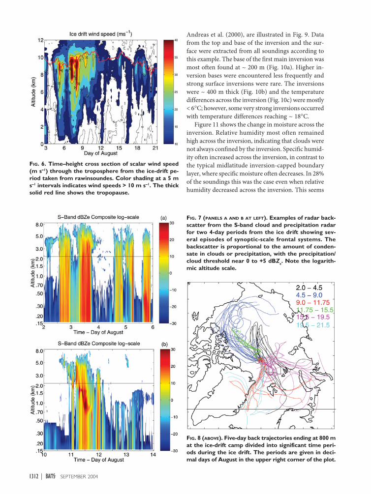
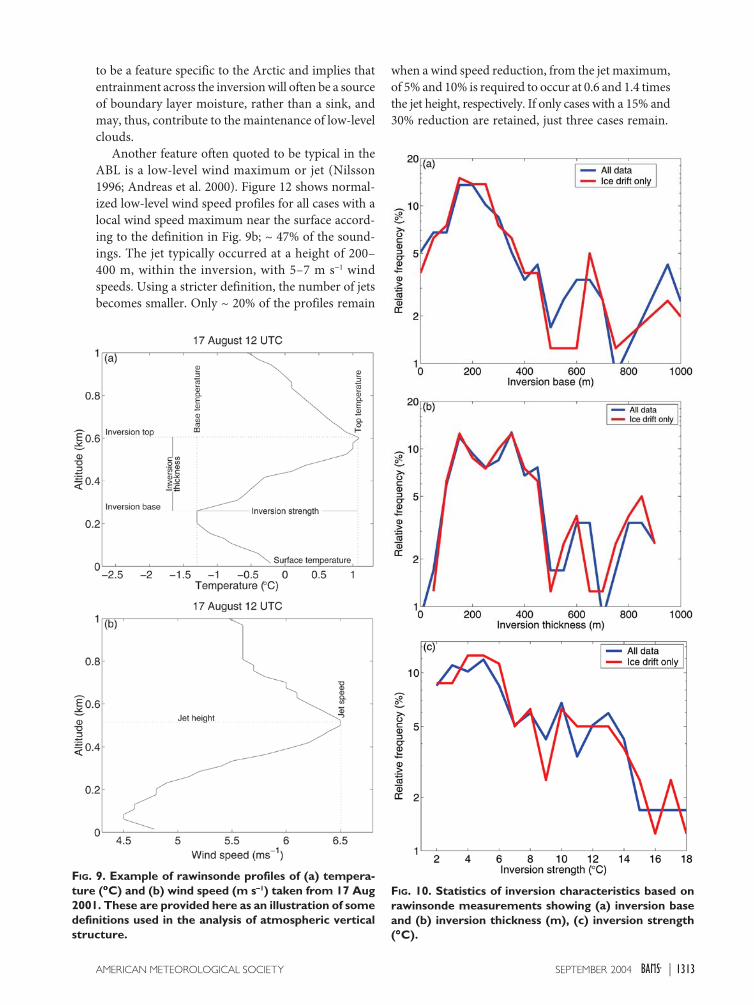
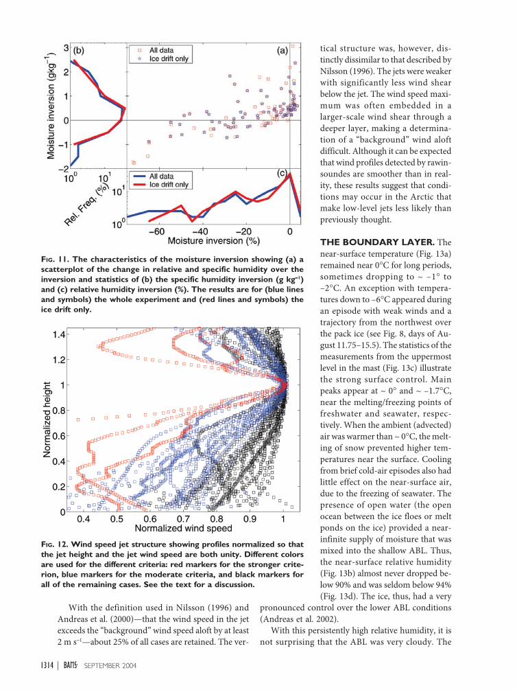
Andreas et al. (2000), are illustrated in Fig. 9. Datafrom the top and base of the inversion and the sur-face were extracted from all soundings according tothis example. The base of the first main inversion wasmost often found at ~ 200 m (Fig. 10a). Higher in-version bases were encountered less frequently andstrong surface inversions were rare. The inversionswere ~ 400 m thick (Fig. 10b) and the temperaturedifferences across the inversion (Fig. 10c) were mostly< 6∞C; however, some very strong inversions occurredwith temperature differences reaching ~ 18∞C.

Figure 11 shows the change in moisture across theinversion. Relative humidity most often remainedhigh across the inversion, indicating that clouds werenot always confined by the inversion. Specific humid-ity often increased across the inversion, in contrast tothe typical midlatitude inversion-capped boundarylayer, where specific moisture often decreases. In 28%of the soundings this was the case even when relativehumidity decreased across the inversion. This seems

FIG. 8 (ABOVE). Five-day back trajectories ending at 800 mat the ice-drift camp divided into significant time peri-ods during the ice drift. The periods are given in deci-mal days of August in the upper right corner of the plot.

FIG. 7 (PANELS A AND B AT LEFT). Examples of radar back-scatter from the S-band cloud and precipitation radarfor two 4-day periods from the ice drift showing sev-eral episodes of synoptic-scale frontal systems. Thebackscatter is proportional to the amount of conden-sate in clouds or precipitation, with the precipitation/cloud threshold near 0 to +5 dBZe. Note the logarith-mic altitude scale.


to be a feature specific to the Arctic and implies thatentrainment across the inversion will often be a sourceof boundary layer moisture, rather than a sink, andmay, thus, contribute to the maintenance of low-levelclouds.

Another feature often quoted to be typical in theABL is a low-level wind maximum or jet (Nilsson1996; Andreas et al. 2000). Figure 12 shows normal-ized low-level wind speed profiles for all cases with alocal wind speed maximum near the surface accord-ing to the definition in Fig. 9b; ~ 47% of the sound-ings. The jet typically occurred at a height of 200–400 m, within the inversion, with 5–7 m s-1 windspeeds. Using a stricter definition, the number of jetsbecomes smaller. Only ~ 20% of the profiles remain

when a wind speed reduction, from the jet maximum,of 5% and 10% is required to occur at 0.6 and 1.4 timesthe jet height, respectively. If only cases with a 15% and30% reduction are retained, just three cases remain.

FIG. 9. Example of rawinsonde profiles of (a) tempera-ture (∞∞∞∞∞C) and (b) wind speed (m s-----1) taken from 17 Aug2001. These are provided here as an illustration of somedefinitions used in the analysis of atmospheric verticalstructure.

FIG. 10. Statistics of inversion characteristics based onrawinsonde measurements showing (a) inversion baseand (b) inversion thickness (m), (c) inversion strength(∞∞∞∞∞C).


tical structure was, however, dis-tinctly dissimilar to that described byNilsson (1996). The jets were weakerwith significantly less wind shearbelow the jet. The wind speed maxi-mum was often embedded in alarger-scale wind shear through adeeper layer, making a determina-tion of a “background” wind aloftdifficult. Although it can be expectedthat wind profiles detected by rawin-soundes are smoother than in real-ity, these results suggest that condi-tions may occur in the Arctic thatmake low-level jets less likely thanpreviously thought.

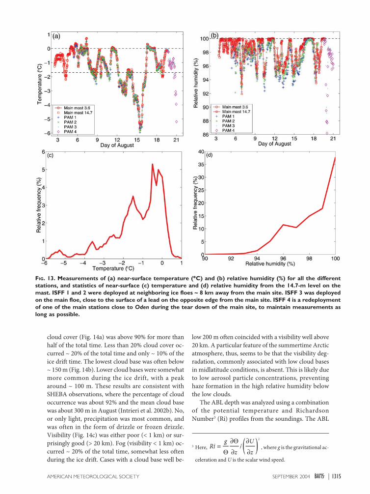
THE BOUNDARY LAYER. Thenear-surface temperature (Fig. 13a)remained near 0∞C for long periods,sometimes dropping to ~ –1∞ to–2∞C. An exception with tempera-tures down to –6∞C appeared duringan episode with weak winds and atrajectory from the northwest overthe pack ice (see Fig. 8, days of Au-gust 11.75–15.5). The statistics of themeasurements from the uppermostlevel in the mast (Fig. 13c) illustratethe strong surface control. Mainpeaks appear at ~ 0∞ and ~ –1.7∞C,near the melting/freezing points offreshwater and seawater, respec-tively. When the ambient (advected)air was warmer than ~ 0∞C, the melt-ing of snow prevented higher tem-peratures near the surface. Coolingfrom brief cold-air episodes also hadlittle effect on the near-surface air,due to the freezing of seawater. Thepresence of open water (the openocean between the ice floes or meltponds on the ice) provided a near-infinite supply of moisture that wasmixed into the shallow ABL. Thus,the near-surface relative humidity(Fig. 13b) almost never dropped be-low 90% and was seldom below 94%(Fig. 13d). The ice, thus, had a very

pronounced control over the lower ABL conditions(Andreas et al. 2002).

With this persistently high relative humidity, it isnot surprising that the ABL was very cloudy. The

FIG. 11. The characteristics of the moisture inversion showing (a) ascatterplot of the change in relative and specific humidity over theinversion and statistics of (b) the specific humidity inversion (g kg-----1)and (c) relative humidity inversion (%). The results are for (blue linesand symbols) the whole experiment and (red lines and symbols) theice drift only.

With the definition used in Nilsson (1996) andAndreas et al. (2000)—that the wind speed in the jetexceeds the “background” wind speed aloft by at least2 m s-1—about 25% of all cases are retained. The ver-

FIG. 12. Wind speed jet structure showing profiles normalized so thatthe jet height and the jet wind speed are both unity. Different colorsare used for the different criteria: red markers for the stronger crite-rion, blue markers for the moderate criteria, and black markers forall of the remaining cases. See the text for a discussion.


cloud cover (Fig. 14a) was above 90% for more thanhalf of the total time. Less than 20% cloud cover oc-curred ~ 20% of the total time and only ~ 10% of theice drift time. The lowest cloud base was often below~ 150 m (Fig. 14b). Lower cloud bases were somewhatmore common during the ice drift, with a peakaround ~ 100 m. These results are consistent withSHEBA observations, where the percentage of cloudoccurrence was about 92% and the mean cloud basewas about 300 m in August (Intrieri et al. 2002b). No,or only light, precipitation was most common, andwas often in the form of drizzle or frozen drizzle.Visibility (Fig. 14c) was either poor (< 1 km) or sur-prisingly good (> 20 km). Fog (visibility < 1 km) oc-curred ~ 20% of the total time, somewhat less oftenduring the ice drift. Cases with a cloud base well be-

low 200 m often coincided with a visibility well above20 km. A particular feature of the summertime Arcticatmosphere, thus, seems to be that the visibility deg-radation, commonly associated with low cloud basesin midlatitude conditions, is absent. This is likely dueto low aerosol particle concentrations, preventinghaze formation in the high relative humidity belowthe low clouds.

The ABL depth was analyzed using a combinationof the potential temperature and RichardsonNumber3 (Ri) profiles from the soundings. The ABL

3 Here, , where g is the gravitational ac-

celeration and U is the scalar wind speed.

FIG. 13. Measurements of (a) near-surface temperature (∞∞∞∞∞C) and (b) relative humidity (%) for all the differentstations, and statistics of near-surface (c) temperature and (d) relative humidity from the 14.7-m level on themast. ISFF 1 and 2 were deployed at neighboring ice floes ~ 8 km away from the main site. ISFF 3 was deployedon the main floe, close to the surface of a lead on the opposite edge from the main site. ISFF 4 is a redeploymentof one of the main stations close to Oden during the tear down of the main site, to maintain measurements aslong as possible.


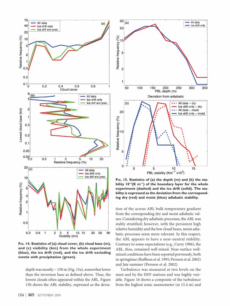
depth was mostly ~ 150 m (Fig. 15a), somewhat lowerthan the inversion base as defined above. Thus, thelowest clouds often appeared within the ABL. Figure15b shows the ABL stability, expressed as the devia-

tion of the across-ABL bulk temperature gradientfrom the corresponding dry and moist adiabatic val-ues. Considering dry adiabatic processes, the ABL wasstably stratified; however, with the persistent highrelative humidity and the low cloud bases, moist adia-batic processes seem more relevant. In this respect,the ABL appears to have a near-neutral stability.Contrary to some expectations (e.g., Curry 1986), theABL, thus, remained well mixed. Near-surface well-mixed conditions have been reported previously, bothin springtime (Ruffieux et al. 1995; Persson et al. 2002)and late summer (Persson et al. 2002).

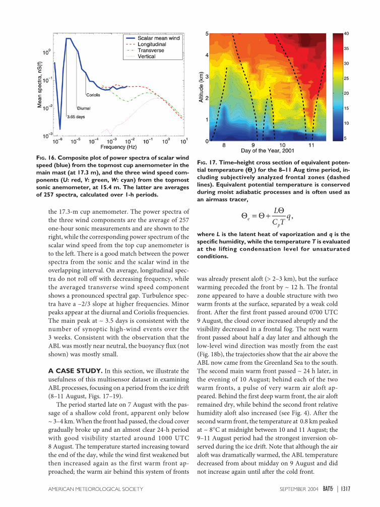
Turbulence was measured at two levels on themast and by the ISFF stations and was highly vari-able. Figure 16 shows a composite of the turbulencefrom the highest sonic anemometer (at 15.4 m) and

FIG. 15. Statistics of (a) the depth (m) and (b) the sta-bility 10-----3(K m-----1) of the boundary layer for the wholeexperiment (dashed) and the ice drift (solid). The sta-bility is expressed as the deviation from the correspond-ing dry (red) and moist (blue) adiabatic stability.

FIG. 14. Statistics of (a) cloud cover, (b) cloud base (m),and (c) visibility (km) from the whole experiment(blue), the ice drift (red), and the ice drift excludingevents with precipitation (green).


the 17.3-m cup anemometer. The power spectra ofthe three wind components are the average of 257one-hour sonic measurements and are shown to theright, while the corresponding power spectrum of thescalar wind speed from the top cup anemometer isto the left. There is a good match between the powerspectra from the sonic and the scalar wind in theoverlapping interval. On average, longitudinal spec-tra do not roll off with decreasing frequency, whilethe averaged transverse wind speed componentshows a pronounced spectral gap. Turbulence spec-tra have a –2/3 slope at higher frequencies. Minorpeaks appear at the diurnal and Coriolis frequencies.The main peak at ~ 3.5 days is consistent with thenumber of synoptic high-wind events over the3 weeks. Consistent with the observation that theABL was mostly near neutral, the buoyancy flux (notshown) was mostly small.

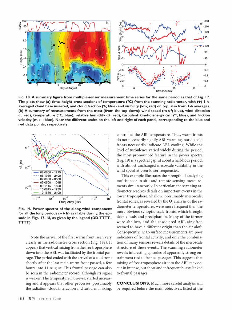
A CASE STUDY. In this section, we illustrate theusefulness of this multisensor dataset in examiningABL processes, focusing on a period from the ice drift(8–11 August, Figs. 17–19).

The period started late on 7 August with the pas-sage of a shallow cold front, apparent only below~ 3–4 km. When the front had passed, the cloud covergradually broke up and an almost clear 24-h periodwith good visibility started around 1000 UTC8 August. The temperature started increasing towardthe end of the day, while the wind first weakened butthen increased again as the first warm front ap-proached; the warm air behind this system of fronts

was already present aloft (> 2–3 km), but the surfacewarming preceded the front by ~ 12 h. The frontalzone appeared to have a double structure with twowarm fronts at the surface, separated by a weak coldfront. After the first front passed around 0700 UTC9 August, the cloud cover increased abruptly and thevisibility decreased in a frontal fog. The next warmfront passed about half a day later and although thelow-level wind direction was mostly from the east(Fig. 18b), the trajectories show that the air above theABL now came from the Greenland Sea to the south.The second main warm front passed ~ 24 h later, inthe evening of 10 August; behind each of the twowarm fronts, a pulse of very warm air aloft ap-peared. Behind the first deep warm front, the air aloftremained dry, while behind the second front relativehumidity aloft also increased (see Fig. 4). After thesecond warm front, the temperature at 0.8 km peakedat ~ 8∞C at midnight between 10 and 11 August; the9–11 August period had the strongest inversion ob-served during the ice drift. Note that although the airaloft was dramatically warmed, the ABL temperaturedecreased from about midday on 9 August and didnot increase again until after the cold front.

FIG. 16. Composite plot of power spectra of scalar windspeed (blue) from the topmost cup anemometer in themain mast (at 17.3 m), and the three wind speed com-ponents (U: red, V: green, W: cyan) from the topmostsonic anemometer, at 15.4 m. The latter are averagesof 257 spectra, calculated over 1-h periods.

FIG. 17. Time–height cross section of equivalent poten-tial temperature (QQQQQe) for the 8–11 Aug time period, in-cluding subjectively analyzed frontal zones (dashedlines). Equivalent potential temperature is conservedduring moist adiabatic processes and is often used asan airmass tracer,

where L is the latent heat of vaporization and q is thespecific humidity, while the temperature T is evaluatedat the lifting condensation level for unsaturatedconditions.


Note the arrival of the first warm front, seen veryclearly in the radiometer cross section (Fig. 18a). Itappears that vertical mixing from the free tropospheredown into the ABL was facilitated by the frontal pas-sage. The period ended with the arrival of a cold frontshortly after the last main warm front passed, a fewhours into 11 August. This frontal passage can alsobe seen in the radiometer record, although its signalis weaker. The temperature, however, started increas-ing and it appears that other processes, presumablythe radiation–cloud interaction and turbulent mixing,

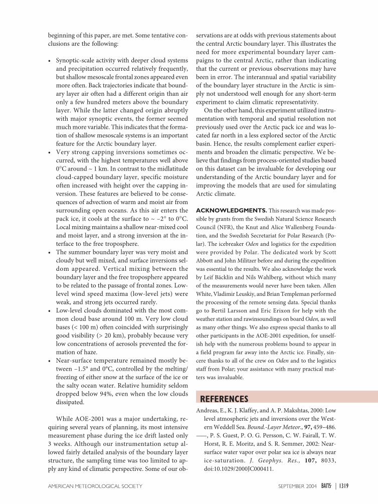
controlled the ABL temperature. Thus, warm frontsdo not necessarily signify ABL warming, nor do coldfronts necessarily indicate ABL cooling. While thelevel of turbulence varied widely during the period,the most pronounced feature in the power spectra(Fig. 19) is a spectral gap, at about a half-hour period,with almost unchanged mesoscale variability in thewind speed at even lower frequencies.

This example illustrates the strength of analyzingmultisensor in situ and remote sensing measure-ments simultaneously. In particular, the scanning ra-diometer resolves details on important events in thelower troposphere. Shallow, presumably mesoscale,frontal zones, as revealed by the Qe analysis or the ra-diometer temperatures, were more frequent than themore obvious synoptic-scale fronts, which broughtdeep clouds and precipitation. Many of the formerwere shallow, and the associated ABL air oftenseemed to have a different origin than the air aloft.Consequently, near-surface measurements are poorindicators of frontal activity, and only the combina-tion of many sensors reveals details of the mesoscalestructure of these events. The scanning radiometerreveals interesting episodes of apparently strong en-trainment tied to frontal passages. This suggests thatmixing of free-troposphere air into the ABL may oc-cur in intense, but short and infrequent bursts linkedto frontal passages.

CONCLUSIONS. Much more careful analysis willbe required before the main objectives, listed at the

FIG. 19. Power spectra of the along-wind componentfor all the long periods (~ 6 h) available during the epi-sode in Figs. 17–18, as given by the legend (DD-TTTT–TTTT).

FIG. 18. A summary figure from multiple-sensor measurement time series for the same period as that of Fig. 17.The plots show (a) time–height cross sections of temperature (∞∞∞∞∞C) from the scanning radiometer, with (∑∑∑∑∑) 1-h-averaged cloud base inserted, and cloud fraction (%; blue) and visibility (km; red) on top, also from 1-h averages.(b) A summary of measurements from the mast (from the top down): wind speed (m s-----1; blue), wind direction(∞∞∞∞∞; red), temperature (∞∞∞∞∞C; blue), relative humidity (%; red), turbulent kinetic energy (m2 s-----2; blue), and frictionvelocity (m s-----1; blue). Note the different scales on the left and right of each panel, corresponding to the blue andred data points, respectively.


beginning of this paper, are met. Some tentative con-clusions are the following:

• Synoptic-scale activity with deeper cloud systemsand precipitation occurred relatively frequently,but shallow mesoscale frontal zones appeared evenmore often. Back trajectories indicate that bound-ary layer air often had a different origin than aironly a few hundred meters above the boundarylayer. While the latter changed origin abruptlywith major synoptic events, the former seemedmuch more variable. This indicates that the forma-tion of shallow mesoscale systems is an importantfeature for the Arctic boundary layer.

• Very strong capping inversions sometimes oc-curred, with the highest temperatures well above0∞C around ~ 1 km. In contrast to the midlatitudecloud-capped boundary layer, specific moistureoften increased with height over the capping in-version. These features are believed to be conse-quences of advection of warm and moist air fromsurrounding open oceans. As this air enters thepack ice, it cools at the surface to ~ –2∞ to 0∞C.Local mixing maintains a shallow near-mixed cooland moist layer, and a strong inversion at the in-terface to the free troposphere.

• The summer boundary layer was very moist andcloudy but well mixed, and surface inversions sel-dom appeared. Vertical mixing between theboundary layer and the free troposphere appearedto be related to the passage of frontal zones. Low-level wind speed maxima (low-level jets) wereweak, and strong jets occurred rarely.

• Low-level clouds dominated with the most com-mon cloud base around 100 m. Very low cloudbases (< 100 m) often coincided with surprisinglygood visibility (> 20 km), probably because verylow concentrations of aerosols prevented the for-mation of haze.

• Near-surface temperature remained mostly be-tween –1.5° and 0°C, controlled by the melting/freezing of either snow at the surface of the ice orthe salty ocean water. Relative humidity seldomdropped below 94%, even when the low cloudsdissipated.

While AOE-2001 was a major undertaking, re-quiring several years of planning, its most intensivemeasurement phase during the ice drift lasted only3 weeks. Although our instrumentation setup al-lowed fairly detailed analysis of the boundary layerstructure, the sampling time was too limited to ap-ply any kind of climatic perspective. Some of our ob-

servations are at odds with previous statements aboutthe central Arctic boundary layer. This illustrates theneed for more experimental boundary layer cam-paigns to the central Arctic, rather than indicatingthat the current or previous observations may havebeen in error. The interannual and spatial variabilityof the boundary layer structure in the Arctic is sim-ply not understood well enough for any short-termexperiment to claim climatic representativity.

On the other hand, this experiment utilized instru-mentation with temporal and spatial resolution notpreviously used over the Arctic pack ice and was lo-cated far north in a less explored sector of the Arcticbasin. Hence, the results complement earlier experi-ments and broaden the climatic perspective. We be-lieve that findings from process-oriented studies basedon this dataset can be invaluable for developing ourunderstanding of the Arctic boundary layer and forimproving the models that are used for simulatingArctic climate.

ACKNOWLEDGMENTS. This research was made pos-sible by grants from the Swedish Natural Science ResearchCouncil (NFR), the Knut and Alice Wallenberg Founda-tion, and the Swedish Secretariat for Polar Research (Po-lar). The icebreaker Oden and logistics for the expeditionwere provided by Polar. The dedicated work by ScottAbbott and John Militzer before and during the expeditionwas essential to the results. We also acknowledge the workby Leif Bäcklin and Nils Wahlberg, without which manyof the measurements would never have been taken. AllenWhite, Vladimir Leuskiy, and Brian Templeman performedthe processing of the remote sensing data. Special thanksgo to Bertil Larsson and Eric Erixon for help with theweather station and rawinsoundings on board Oden, as wellas many other things. We also express special thanks to allother participants in the AOE-2001 expedition, for unself-ish help with the numerous problems bound to appear ina field program far away into the Arctic ice. Finally, sin-cere thanks to all of the crew on Oden and to the logisticsstaff from Polar; your assistance with many practical mat-ters was invaluable.

REFERENCESAndreas, E., K. J. Klaffey, and A. P. Makshtas, 2000: Low

level atmospheric jets and inversions over the West-ern Weddell Sea. Bound.-Layer Meteor., 97, 459–486.

——, P. S. Guest, P. O. G. Persson, C. W. Fairall, T. W.Horst, R. E. Moritz, and S. R. Semmer, 2002: Near-surface water vapor over polar sea ice is always nearice-saturation. J. Geophys. Res., 107, 8033,doi:10.1029/2000JC000411.


Battisti, C. M., C. M. Bitz, and R.M. Moritz, 1997: Dogeneral circulation models underestimate the natu-ral variability in the Arctic climate? J. Climate, 10,1909–1920.

Beesley, J. A., C. S. Bretherton, C. Jacob, E. L Andreas, J.M. Intrieri, and T. A. Uttal, 2000: A comparison ofcloud and boundary layer variables in the ECMWFforecast model with observations at the Surface Heatand Energy of the Arctic (SHEBA) ice camp. J.Geophys. Res., 105 (D10), 12 337–12 349.

Bigg, E. K., and C. Leck, 2001: Cloud-active particlesover the central Arctic area. J. Geophys. Res., 106(D23), 32 155–32 166.

——, ——, and E. D. Nilsson, 1996: Sudden changes inArctic atmospheric aerosol concentrations duringsummer and autumn. Tellus, 48, 254–271.

——, ——, and E. D. Nilsson, 2001: Sudden changes inaerosol and gas concentration in the central Arcticmarine boundary layer: Causes and consequences. J.Geophys. Res., 106 (D23), 32 167–32 185.

Chapman, W. L., and J. E. Walsh, 1993: Recent varia-tions of sea ice and air temperature in high latitudes.Bull. Amer. Meteor. Soc., 74, 33–47.

Comiso, J. C., 2002: A rapidly declining perennial seaice cover in the Arctic. Geophys. Res. Lett., 29, 1956,doi:10.1029/2002GL015650.

Curry, J. A., 1986: Interactions among turbulence, radia-tion and microphysics in Arctic stratus clouds. J.Atmos. Sci., 43, 90–106.

——, and Coauthors, 2000: FIRE Arctic clouds experi-ment. Bull. Amer. Meteor. Soc., 81, 5–29.

Grachev, A. A., C. W. Fairall, P. O. G. Persson, E. LAndreas, and P. S. Guest, 2004: Stable boundary-layerscaling regimes: The SHEBA data. Bound.-LayerMeteor., in press.

Houghton, J. T., Y. Ding, D. J. Griggs, M. Nogner, P. J.van der Linden, X. Dai, K. Maskell, and C. C.Johnson, Eds., 2001: Climate Change 2001: The Sci-entific Basis. IPCC Rep., 881 pp.

Intrieri, J. M., C. W. Fairall, M. D. Shupe, P. O. G.Persson, E. L Andreas, P. S. Guest, and R. E. Moritz,2002a: An annual cycle of Arctic surface cloud forc-ing at SHEBA. J. Geophys. Res., 107, 8039,doi:10.1029/2000JC000439.

——, M. D. Shupe, T. Uttal, and B. J. McCarty, 2002b:An annual cycle of Arctic clouds characteristics ob-served by radar and lidar at SHEBA. J. Geophys. Res.,107, 8030, doi:10.1029/2000JC000423.

Kahl, J. D., N. A. Zaitseva, V. Khattatov, R. C. Schnell,D. M. Bacon, J. Bacon, V. Radionov, and M. C. Serreze,1999: Radiosonde observations from the formerSoviet “North Pole” series of drifting ice stations,1954–90. Bull. Amer. Meteor. Soc., 80, 2019–2026.

Kalnay, E., and Coauthors, 1996: The NCEP/NCAR 40-Year Reanalysis Project. Bull. Amer. Meteor. Soc., 77,437–471.

Leck, C., and C. Persson, 1996: Seasonal and short-termvariability in dimethyl sulfide, sulfur dioxide and bio-genic sulfur and sea salt aerosol particles in the arc-tic marine boundary layer, during summer and au-tumn. Tellus, 48B, 272–299.

——, and E. K. Bigg, 1999: Aerosol production over re-mote marine areas—A new route. Geophys. Res. Lett.,26, 3577–3580.

——, ——, D. S. Covert, J. Heintzenberg, W. Maenhaut,E. D. Nilsson, and A. Wiedensohler, 1996: Overviewof the atmospheric research program during the In-ternational Ocean Expedition of 1991 (IAOE-1991)and its scientific results. Tellus, 48B, 136–155.

——, E. D. Nilsson, E. K. Bigg, and L. Bäcklin, 2001a: Theatmospheric program of the Arctic Ocean Expedition1996 (AOE-1996)—An overview of scientific objec-tives, experimental approaches and instruments. J.Geophys. Res., 106 (D23), 32 051–32 067.

——, M. Norman, E. K. Bigg, and R. Hillamo, 2001b:Chemical composition and sources of the high Arc-tic aerosol relevant for cloud formation. J. Geophys.Res., 107 (D12), 1–17, doi:10.1029/2001JD001463.

——, M. Tjernström, P. Matrai, E. Swietlicki, and E. K.Bigg, 2004: Can marine microorganisms influencemelting of the Arctic pack ice. Eos, Trans. Amer.Geophys. Union, 85, 25–36.

Mahrt, L., 1998: Stratified atmospheric boundary layersand breakdown of models. Theor. Comput. FluidDyn., 11, 263–279.

McGrath, 1989: Trajectory models and their use in theIrish Meteorological Service. Irish MeteorologicalService, Tech. Memo. 112/89, 12 pp.

Meehl, G. A., G. J. Boer, C. Covey, M. Latif, and R. J.Stouffer, 2000: The Coupled Model IntercomparisonProject (CMIP). Bull. Amer. Meteor. Soc., 81, 313–318.

Morison, J. H., K. Aagaard, and M. Steele, 2000: Recentenvironmental changes in the Arctic: A review. Arc-tic, 53, 4.

Nilsson, E. D., 1996: Planetary boundary layer structureand air mass transport during the InternationalArctic Ocean Expedition 1991. Tellus, 48B, 178–196.

Parkinson, C., D. J. Cavalieri, P. Gloersen, H. J. Zwally,and J. C. Comiso, 1999: Arctic sea ice extents, areas,and trends, 1978–1996. J. Geophys. Res., 104, 20 837–20 856.

Perovich, D. K., and Coauthors, 1999: Year on ice givesclimate insights. Eos, Trans. Amer. Geophys. Union,80, 483–486.

Persson, P. O. G., C. W. Fairall, E. L Andreas, P. S. Guest,and D. K. Perovich, 2002: Measurements near the At-


mospheric Surface Flux Group tower at SHEBA: Near-surface conditions and surface energy budget. J.Geophys. Res., 107, 8045, doi:10.1029/2000JC000705.

Persson, P. O. G., E. L Andreas, C. W. Fairall, P. S. Guest,and D. K. Perovich, 2003: Pack ice surface energychanges at SHEBA initiated by late summer synop-tic forcing. Preprints, Seventh Conf. on Polar Meteo-rology and Oceanography and Joint Symp. on High-Latitude Climate Variations, Hyannis, MA, Amer.Meteor. Soc., CD-ROM 3.21.

Räisänen, J., 2001: CO2-induced climate change in theArctic area in the CMIP2 experiments. SWECLIMNewsletter, Vol. 11, 23–28. [Available from SwedishMeteorological and Hydrological Institute, SE-601 76Norrköping, Sweden.]

Rigor, I. G., R. L. Colony, and S. Martin, 2000: Variationsin surface air temperature observations in the Arc-tic, 1979–97. J. Climate, 13, 896–914.

Ruffieux, D. R., P. O. G. Persson, C. W. Fairall, and DanE. Wolfe, 1995: Ice pack and lead surface energy bud-

gets during LEADEX 92. J. Geophys. Res., 100 (C3),4593–4612.

Serreze, M. C., and Coauthors, 2000: Observational evi-dence of recent change in the northern high-latitudeenvironment. Climate Change, 46, 159–207.

Thompson, D. W. J., and J. M. Wallace, 1998: The Arc-tic Oscillation signature in the wintertimegeopotential height and temperature fields. Geophys.Res. Lett., 25, 1297–1300.

Tjernström, M., C. Leck, P. O. G. Persson, M. L. Jensen,S. P. Oncley, and A. Targino, 2004: Experimentalequipment. Bull. Amer. Meteor. Soc., 85, doi:10.1175-BAMS-85-9-Tjernstrom.

Uttal, T., and Coauthors, 2002: Surface Heat Budget ofthe Arctic Ocean. Bull. Amer. Meteor. Soc., 83, 255–276.

Walsh, J. E., W. M. Kattsov, W. L. Chapman,V. Govorkova, and T. Pavlova, 2002: Comparison ofArctic climate by uncoupled and coupled globalmodels. J. Climate, 15, 1429–1446.

Documents

THE SUMMERTIME ARCTIC ATMOSPHERERussian drifting North Pole stations were also made available (e.g., Kahl et al. 1999). The atmospheric program during the summer of 2001 [Arctic Ocean