Embed Size (px)
Citation preview

HAL Id: tel-01315224https://tel.archives-ouvertes.fr/tel-01315224
Submitted on 12 May 2016
HAL is a multi-disciplinary open accessarchive for the deposit and dissemination of sci-entific research documents, whether they are pub-lished or not. The documents may come fromteaching and research institutions in France orabroad, or from public or private research centers.
L’archive ouverte pluridisciplinaire HAL, estdestinée au dépôt et à la diffusion de documentsscientifiques de niveau recherche, publiés ou non,émanant des établissements d’enseignement et derecherche français ou étrangers, des laboratoirespublics ou privés.
The study of phase separation in the miscibility gap andion specific effects on the aggregation of soft matter
systemLi Zhang
To cite this version:Li Zhang. The study of phase separation in the miscibility gap and ion specific effects on the ag-gregation of soft matter system. Soft Condensed Matter [cond-mat.soft]. Université Paris Saclay(COmUE); Northwestern Polytechnical University (Chine), 2016. English. �NNT : 2016SACLS106�.�tel-01315224�

NNT : 2016SACLS106
THESE DE DOCTORAT DE
NORTHWESTERN POLYTECHNICAL UNIVERSITY
ET DE L’UNIVERSITE PARIS-SACLAY
PREPAREE A L’UNIVERSITE PARIS-SUD
ÉCOLE DOCTORALE N°564
PHYSIQUE EN ILE-DE-FRANCE
Spécialité de doctorat : PHYSIQUE
Par
Mme Li Zhang
The study of phase separation in the miscibility gap and ion specific effects on the
aggregation of soft matter systems Thèse présentée et soutenue à Xi’an, le 7 Avril 2016 :
Composition du Jury : Mme Y. P. Zheng M. J. Oberdisse M. W. X. Chen M. F. Muller Mme. A. Salonen M. N. Wang
Dr, Northwestern Polytechnical University Dr, Université de Montpellier Dr, Xi’an Technological University Dr, ECE-PARIS Dr, Université Paris-sud, Université Paris Saclay Professeur, Northwestern Polytechnical University
Présidente du Jury Rapporteur Rapporteur Examinatrice Directeur de thèse Directeur de thèse

Acknowledgements
1
Acknowledgements
I would like to extend my sincere gratitude to Prof. Nan Wang and Prof. Anniina
Salonen for their instructive advice and patience throughout my thesis. This thesis is
finished under their professional suggestions and inspiring encouragements. Their
profound understanding in phase transition, foam and colloidal science has helped me
a lot in designing the ideas and experiments scientifically. Their enthusiasm for
scientific research always encourages me to solve the difficulties conquered during
the experimental process and data analysis.
Thank Prof. Nan Wang for giving me the opportunity to study in abroad, and
Prof. Dominique Langevin and Prof. Anniina Salonen for offering me the chance to
perform the research in Laboratoire de Physique des solides.
I really feel lucky that I am surrounded by the intelligent and lovely mates in the
labs in China and France. I have benefited greatly from Prof. Anniina Salonen for
providing me the chance to study the fascinating topic in LPS, for the experimental
guidance, instrumental set up and use, data discussion and interpretation, valuable
suggestions on the preparation for the conference, as well as for caring my daily life

Acknowledgements
2
in France, from Prof. Nan Wang for providing me an interesting topic through which I
trained how to do scientific work, for persisting guidance on learning to think,
experimental equipment design and data analysis, from Prof. Dominique Langevin,
Prof. Doru Constantin, Prof. Giuseppe Foffi, Prof. François Muller, Prof. Fabrice
Cousin, Dr. Alesya Mikhailovskaya, Dr. Joseph Tavacoli and Dr. Pavel Yazhgur for
their valuable discussion and suggestions, from Dr. Julien Schmitt, and Dr. Cyrille
Rochas for their helping in the SAXS experiment, from Dr. Delphine Hannoy for the
surface tension measurement, From Zenaida Cenorina I.Q.UAN and Clément
Honorez for helping in using rheometer, from Dr. Delphine Hannoy for teaching me
in doing Zeta Potential measurement, from Dr. Eric Raspaud for generously letting me
use the light scattering equipment, from Dr. Yin Li Peng and Liang Zhang for helping
in the transparent system experiment.
I would like to thank Lorène Champougny, Wiebke Drenckhan, Emilie Forel,
Thibaut Gaillard, Anaïs Giustiniani, Emmanuelle Rio, Matthieu Roche for being
dedicated lab mates. Gratitude is extended to Lin Ji, Lei Wang, Li Li tian, Huan Yang,
Yang Bai, Tong Qi Wen, Jia Chen Guo, Yun Fei Li for the support in my daily life and
work.
Finally, I would like to give my warmly thanks to my parents, young brother and
boyfriend for their permanent encouragement and immerse support in these years.
Moreover, I am sincerely grateful for all my friends both in China and France, thanks
for their helping when I met problems and cherishing the good memory we were
together.
The thesis is supported by Doctorate Foundation of Northwestern Polytechnical
University, the European Space Agency (MAP Hydrodynamics of wet foams),
partially funded by ESA and the European Infrastructure Network QualityNano, and
the China Scholarship Council.
Contents
Contents
Acknowledgements................................................................................................... 1
Chapter 1 Introduction ............................................................................................. 6
Chapter 2 Background ........................................................................................... 10
2.1 Phase behavior in miscibility gap ................................................................... 10
2.1.1 Thermodynamics of liquid-liquid phase separation ..........................................11
2.1.2 Kinetics of liquid-liquid phase separation: Nucleation growth and spinodal
decomposition ................................................................................................... 13
2.1.3 Schematic phase diagram type of the systems with miscibility gap ................... 15
2.1.4 Marangoni force ........................................................................................ 16
2.2 Colloidal gels .................................................................................................. 17
2.2.1 DLVO theory............................................................................................. 18
2.2.2 Gel structure.............................................................................................. 19
2.3 Foam................................................................................................................ 21
2.3.1 Surfactants ................................................................................................ 21
2.3.2 Foam structure........................................................................................... 22
2.3.3 Foam aging ............................................................................................... 23
2.3.4 Slowing down the ageing of foam ................................................................ 24
2.4 Hofmeister series............................................................................................. 25
2.4.1 Ions at interface ......................................................................................... 26
2.4.2 Interactions between colloidal partic les in the presence of electrolyte ............... 27
Chapter 3 Materials and methods........................................................................ 29
3.1 Materials.......................................................................................................... 29
3.1.1 Phase separation ........................................................................................ 29

Contents
3.1.2 Gels ......................................................................................................... 29
3.1.3 Foam ........................................................................................................ 30
3.1.4 Gel foam................................................................................................... 30
3.2 Methods........................................................................................................... 31
3.2.1 Sample preparation in miscibility gap and calculation ..................................... 31
3.2.2 Gel sample preparation and measurements .................................................... 33
3.2.3 Foam sample preparation and stability studies ............................................... 35
3.2.4 Foam aging with gel phase .......................................................................... 39
Chapter 4 Phase separation mechanisms studied in miscibility gap .......... 41
4.1 Introduction ..................................................................................................... 41
4.2 Results and discussion .................................................................................... 42
4.2.1 Phase separation of SCN-H2O system in a uni-directional temperature field ...... 42
4.2.2 Phase separation of SCN-H2O system at isothermal field ................................ 47
4.2.3 Growth rate and volume fraction of minority phase to the effect of the
microstructure ................................................................................................... 50
4.2.4 The probability of produced muti-layer structure ............................................ 51
4.2.5 The phase separation pattern to the effect of the solidif ied structure .................. 52
4.3 Conclusions ..................................................................................................... 54
Chapter 5 Influence of salt type on gelation kinetics (NaCl or KCl) ......... 56
5.1 Introduction ..................................................................................................... 56
5.2 Results and discussion .................................................................................... 58
5.2.1 Gel General observations and phase diagrams................................................ 58
5.2.2 Gel structure.............................................................................................. 60
5.2.3 Kinetics .................................................................................................... 62
5.2.4 Scaling ..................................................................................................... 65
5.2.5 Gel rheology at a given time ........................................................................ 70
5.3 Conclusions ..................................................................................................... 72
Chapter 6 Influence of different salts on the gelation kinetics .................... 73
6.1 Introduction ..................................................................................................... 73
6.2 Results and discussion .................................................................................... 75
6.2.1 General observation of gel samples .............................................................. 75
6.2.2 The scaling behavior .................................................................................. 76
6.2.3 Half-time of the transmitted intensity............................................................ 79
6.2.4 Stability of the gel system ........................................................................... 81
6.3 Conclusions ..................................................................................................... 83
Chapter 7 Mix salt and surfactant to make ultrastable and stimulable foam
...................................................................................................................................... 85
7.1 Introduction ..................................................................................................... 85
7.2 Results and discussion .................................................................................... 86
7.2.1 Foamability and foam stability with fixed SDS at room temperature ................. 86

Contents
7.2.2 Influence of changing SDS concentration on foam generation and stability........ 89
7.2.3 Kinetics of crystals formation ...................................................................... 93
7.2.4 Structure of crystallites inside the foam......................................................... 95
7.2.5 Stimulating the foam by temperature ............................................................ 97
7.3 Conclusions ..................................................................................................... 99
Chapter 8 Foam aging modified by the gel phase..........................................100
8.1 Introduction ....................................................................................................100
8.2 Results and discussion ...................................................................................101
8.2.1 The evolution of bubbles in the gel foam......................................................101
8.2.2 The mechanical properties of the bulk gel phase............................................105
8.2.3 The effect of gel strength on foam aging ......................................................106
8.2.4 Correlation behavior ..................................................................................108
8.2.5 Small angle Neutron Scattering measurements .............................................. 110
8.3 Conclusions .................................................................................................... 116
Chapter 9 Conclusions .......................................................................................... 118
Bibliography ............................................................................................................121
Appendix Resumé substantiel de la thèse ........................................................132

Chapter 1 Introduction
Chapter 1 Introduction
Many common industrial products and processes are composed of multiple
phases that are incompatible. Depending on the processes the systems can be required
to remain separate, such as foams and emulsions (mixtures of gas and fluid or 2 fluids)
where the dispersions are stabilized through the use of interfacial active molecules or
particles. Such systems also include particulate suspensions (such as paints, paper,
soil, clays and so on), which are often stabilised by surface charges. However, in other
cases the mixtures are not stabilised and phase separation occurs through coarsening.
The phase separation process can be important as it determines the structure of the
final material. For example, metal alloys with special microstructure are made by
cooling from a temperature above the melting temperature, similarly to many polymer
systems. Meanwhile, particles can aggregate as the solid phase comes out.
There is a wide range of systems that exhibit phase separation and my thesis has
concentrated on the study of various types of such systems. I have studied the phase
separation of a transparent system in the miscibility gap in China, but in 09.2013 as I
got the opportunity to spend one and a half years in France as part of my studies I
concentrated on slightly different systems. My project is to study the ion specific

Chapter 1 Introduction
effects on the aggregation of soft matter systems. Therefore, in my thesis, Chapter 4 is
my work in China and Chapter 5, 6, 7 and 8 are the work in France.
My work in China concentrated on studying the phase separation in the
miscibility gap. When the temperature is quenched into the miscibility gap, a phase
separation process occurred. Which is either nucleation growth (NG) or spinodal
decomposition (SD). The study of the phase separation pattern in the miscibility gap
is significant from a practical viewpoint for providing a novel approach to create
special regular microstructures. This suggests that it is necessary to study the
evolution of microstructure under certain conditions and formation kinetics of
minority phase. In this dissertation, a transparent system with a miscibility gap is used
to investigate the aging of microstructure for SD and NG type with the thermal
gradient and the growth rate of minority phase with isothermal field.
In France I worked on making stable foam through the formation of a gel inside
the foam. Adding salt to the dispersion of colloidal particles can lead to aggregation
due to screening of repulsive electrostatic force between particles and make gels,
which have many applications such as in food and material science. It’s important to
know how the gel ages with time, which has already been widely studied. However,
previous studies tend to observe the macroscopic gelation time and using the same
salt at various concentrations when comparing the gel properties. In this dissertation,
we first observe the microscopic gelation time and then compare the gel properties in
the presence of different types of salts.
Obtaining stable foams is an important issue in the view of their large variety of
applications. There are many ways to make stable foams up to now. However, many
of them are complicated. In this dissertation, by adding high concentrations of salt
(NaCl or KCl) to surfactant SDS, ultrastable foam can be made and the foam is
temperature sensitive. In addition, solid foams also have numerous applications due to
their low mass density and high surface area properties. This indicates that it’s
important to know how the aging of bubbles during the foam changes as the
continuous phase goes from a liquid to a solid (gel). In this dissertation, ge l phase is
used to modify the foam stability.
Outline of the thesis is as follows:
Chapter 2 gives an overview of the different concepts that are used in the rest of
Chapter 1 Introduction
the manuscript.
Chapter 3 describes the experimental methods and materials used.
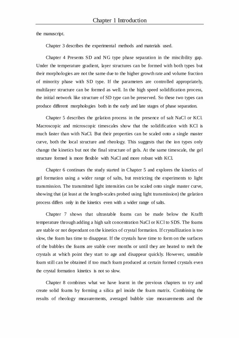
Chapter 4 Presents SD and NG type phase separation in the miscibility gap.
Under the temperature gradient, layer structures can be formed with both types but
their morphologies are not the same due to the higher growth rate and volume fraction
of minority phase with SD type. If the parameters are controlled appropriately,
multilayer structure can be formed as well. In the high speed solidification process,
the initial network like structure of SD type can be preserved. So these two types can
produce different morphologies both in the early and late stages of phase separation.
Chapter 5 describes the gelation process in the presence of salt NaCl or KCl.
Macroscopic and microscopic timescales show that the solidification with KCl is
much faster than with NaCl. But their properties can be scaled onto a single master
curve, both the local structure and rheology. This suggests that the ion types only
change the kinetics but not the final structure of gels. At the same timescale, the gel
structure formed is more flexible with NaCl and more robust with KCl.
Chapter 6 continues the study started in Chapter 5 and explores the kinetics of
gel formation using a wider range of salts, but restricting the experiments to light
transmission. The transmitted light intensities can be scaled onto single master curve,
showing that (at least at the length-scales probed using light transmission) the gelation
process differs only in the kinetics even with a wider range of salts.
Chapter 7 shows that ultrastable foams can be made below the Krafft
temperature through adding a high salt concentration NaCl or KCl to SDS. The foams
are stable or not dependant on the kinetics of crystal formation. If crystallization is too
slow, the foam has time to disappear. If the crystals have time to form on the surfaces
of the bubbles the foams are stable over months or until they are heated to melt the
crystals at which point they start to age and disappear quickly. However, unstable
foam still can be obtained if too much foam produced at certain formed crystals even
the crystal formation kinetics is not so slow.
Chapter 8 combines what we have learnt in the previous chapters to try and
create solid foams by forming a silica gel inside the foam matrix. Combining the
results of rheology measurements, averaged bubble size measurements and the

Chapter 1 Introduction
correlation behavior, we show that the foam aging can be arrested with higher gel
strength and faster gelation time, indicating that the gel strength and gelation kinetics
are two important factors to control the foam stability.
Chapter 2 Background
Chapter 2 Background
2.1 Phase behavior in miscibility gap
The definition of a miscibility gap from the science dictionary is that the region
of temperature and composition in which two kinds of liquids form two layers or
phases when brought together. A miscibility gap in the liquid state exists in a
considerable number of largely different systems such as organic liquids [1],
metal-metal/oxide systems [2, 3], polymer mixtures [4-8], glasses [9], or most
common ingredients to daily experience in cooking, water and oil. The list of
materials being immiscible in the liquid state is endless.
The materials in the miscibility region have a wide range of applications. For
example, immiscible organic liquids are widely used in cosmetic and food industry,
metallic systems are often used as switches, electrical contacts and bearing in car
engines [3], immiscible glasses are mostly used as shock-resistant ceramics,
low-thermal expansion glasses and so on [9].
The phase separation processes in the miscibility gap have a strong effect on the

Chapter 2 Background
final microstructure. Therefore, studying the phase behavior in the miscibility gap can
lead to a better understanding and control of the microstructure.
2.1.1 Thermodynamics of liquid-liquid phase separation
According to the theory of thermodynamics, the system can spontaneously occur
only when the change of Gibbs free energy is less than 0, the liquid- liquid phase
separation obeys this criterion too. In the following we will use the law of regular
solution to discuss the thermodynamic process of liquid- liquid phase separation.
When components A and B exist independently, the free energy of the system is
given by Equation 2.1 as
( )
L L L
A B A A B BG x G x G (2.1)
Where Ax ,
Bx are the molar fractions of A and B respectively; L
AG 、 L
BG are the
molar free energies of A and B; ( )
L
A BG is the molar free energy of the whole system
when A and B are not mixed.
The molar free energy of mixing A and B, at constant temperature T and pressure
P, can be written as
( )
L L
A B mixG G G (2.2)
where mixG is the molar mixing free energy.
According to the Helmholtz-Gibbs Equation, the relationship between molar
mixing free energy mixG and molar mixing enthalpy mixH and molar mixing
entropymixS as
mix mix mixG H T S (2.3)
For a regular solution, mixH can be expressed as
mix A BH x x (2.4)
Where is a coefficient related to the change of free energy and coordination number
when components A and B mixed. Ax and Bx are the molar fraction of A and B, and
satisfy the relationship 1A Bx x . From statistical thermodynamics, we know that
the mixing entropy of the solution can be expressed as

Chapter 2 Background
( ln ln )mix A A B BS R x x x x (2.5)
Where R is the gas constant. Ax and
Bx are smaller than 1, so mixS is always positive.
The mixing free energy mixG is given by Equations (1.3), (1.4) and (1.5) as
A B A A B B( ln + ln )mixG x x RT x x x x (2.6)
The second term on the right of Equation (1.6) is negative, so a value of mixing
free energy higher or lower than 0 depends on the first term. There are two conditions:
(1) For exothermic solutions, the mixing enthalpy 0mixH at all temperatures
and all compositions mixed results in the decrease of the free energy ( 0mixG ). The
system can occur spontaneously.
(2) For the endothermic solutions, the mixing enthalpy 0mixH , and whether
the system can occur spontaneously depends on the temperature and composition of
the system. When the temperature is high, mixT S is higher than
mixH for all the
compositions andmixG is still lower than 0 as shown in Figure 2.1(a). Therefore, the
system still can occur spontaneously. When the temperature is low, for some
compositionsmixT S is higher than
mixH and for some compositionsmixT S is lower
Figure 2.1 The curves of mixing Gibbs-free energy (mixG ) at different temperatures when the
mixing enthalpy ΔH>0, A and B represent two components, Bx represents the molar fraction of
component B, mixS is the molar mixing entropy and T is the temperature. (a) at high temperature,
(b) at low temperature.

Chapter 2 Background
thanmixH , so
mixG is not always lower than 0 at all the compositions as shown in
Figure 2.1(b). In other words, the system cannot occur spontaneously at all the
compositions.
2.1.2 Kinetics of liquid-liquid phase separation: Nucleation growth
and spinodal decomposition
Figure 2.2(a) gives the curve ofmixG plotted versus
Bx at temperature T1. The
points A and B represent the points where the straight dashed red line touch A and B is
tangential to the curve and called the binodal points. All the binodal points at all the
temperatures make the binodal curve, which can be obtained from the Equation
0m
B T
G
x
Put into Equation (1.6) this gives
B
A
xln 0
xA Bx x RT
B
B
B
1- 2x
1- xln
x
T
R
(2.7)
This is the Equation of the binodal curve in a liquid- liquid immiscible gap as
shown in Figure 2.2(b).
The points P and Q are the points of inflection, where the curvature of the curve
mixG changes sign, and are called the spinodal points. All the spinodal points at all
the temperature range assemble the spinodal curve, which can be obtained from the
Equation 2
20m
B T
G
x
Used with Equation (2.6) this gives
A B
1 12 ( + ) 0
x x- RT
B Bx 1- x2
TR
(2.8)
This is the Equation of the spinodal curve in a liquid- liquid immiscible gap as
shown in Figure 2.2(b).
From Figure 2.2 we can see that the spinodal curve separates the liquid- liquid

Chapter 2 Background
misciblility gap into another two regions:
(1) Metastable region: The region between binodal curve and spinodal curve,
where the phase separation pattern is called nucleation growth (NG).
(2) Unstable region: The region surrounded by the spinodal curve, where the
phase separation pattern is called spinodal decomposition (SD).
Figure 2.2 Schematic diagram of ∆Gmix versus XB at temperature T1 (a) and the formed binodal
and spinodal curves (b).
NG type phase separation is associated with metastability, which means that the
existence of an energy barrier, small fluctuations in compositions can lead to the
increase of the free energy. However, it can decrease for larger fluctuations if the
mixture separates into two phases of compositions corresponding to the two points A
and B in Figure 2.2(a). In this condition, domains of a minimum size, of the so-called
critical nucleation radius, are necessary. The concentration profile of NG is illustrated
in Figure 2.3(a) [10], this kind of phase separation mechanism results in domain size
increasing with time and the domains tend to be spherical in nature.
As shown in Figure 2.2(b), SD type phase separation is associated with
instability, which takes place in a completely different way compared with NG type.
Small fluctuations in composition between the point P and Q as shown in Figure 2.2(a)
can lead to the lowest free energy. The concentration profile of SD is illustrated in
Figure 2.3(b), a continuous growth of the amplitude of a concentration fluctuation
Chapter 2 Background
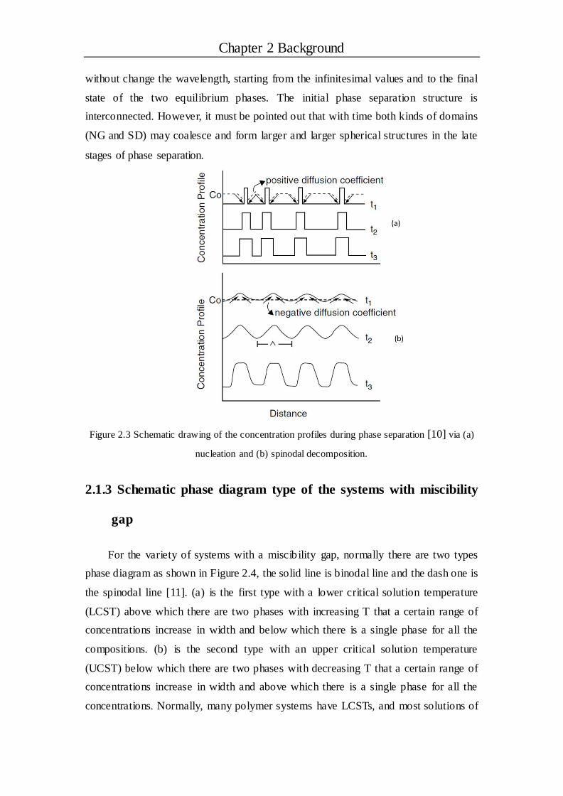
without change the wavelength, starting from the infinitesimal values and to the final
state of the two equilibrium phases. The initial phase separation structure is
interconnected. However, it must be pointed out that with time both kinds of domains
(NG and SD) may coalesce and form larger and larger spherical structures in the late
stages of phase separation.
Figure 2.3 Schematic drawing of the concentration profiles during phase separation [10] via (a)
nucleation and (b) spinodal decomposition.
2.1.3 Schematic phase diagram type of the systems with miscibility
gap
For the variety of systems with a miscibility gap, normally there are two types
phase diagram as shown in Figure 2.4, the solid line is binodal line and the dash one is
the spinodal line [11]. (a) is the first type with a lower critical solution temperature
(LCST) above which there are two phases with increasing T that a certain range of
concentrations increase in width and below which there is a single phase for all the
compositions. (b) is the second type with an upper critical solution temperature
(UCST) below which there are two phases with decreasing T that a certain range of
concentrations increase in width and above which there is a single phase for all the
concentrations. Normally, many polymer systems have LCSTs, and most solutions of

Chapter 2 Background
small molecules have UCSTs. However, more complicated type of behavior with
more than one UCST or LCST or neither type of critical solution temperature are also
observed for polymers.
Figure 2.4 Schematic phase diagrams for mixtures showing binodals and spinodals with (a) lower
and (b) upper critical solution temperature.
2.1.4 Marangoni force
Young, Ratke et al [12-15] showed that in the liquid-liquid miscibility gap if
there is an interfacial tension gradient between the second phase droplets formed
through NG or SD and the matrix phase, the droplets would be pushed to the lower
interfacial energy region by the Marangoni force [15], which results from the
interfacial tension gradient. The resulting terminal velocity of the droplets is given by
x
T
T
rv
md
m
233
2 (2.9)
Where r is the radius of the droplet, d and m are the viscosities of the droplet and
the liquid matrix, is the interfacial energy, T is the temperature, and x is the
distance.

Chapter 2 Background
2.2 Colloidal gels
Colloids are particles that are small enough to be influenced by thermal
fluctuations and not dominated by gravity. This means that they typically have a size
in the range from around 1nm to 1 μm. Colloidal particles are important in many
fields of science and technology, in particular to change the rheological properties of
fluids [16-21]. Often, the dispersed colloidal particles are insoluble in water, but
stabilized to form aqueous dispersions through electrostatic repulsion, which should
be stronger than the Van der Waals attraction.
However, if the suspension is destabilized the particles aggregate and can form a
gel. The basic definition of a gel from Britannica encyclopedia: coherent mass
consisting of a liquid in which particles are either dispersed or arranged in a fine
network throughout the mass. In rheological terms the gel point can be defined as the
point where the Storage modulus (G’) becomes higher than the Loss modulus (G’’)
indicating that the fluid has transitioned from fluid like behavior to solid elastic
behavior [22]. However, the resulting gels can be very different, they can be jellylike
or elastic, or quite solid and rigid (like silica gels) [23].
Previous experiments and theoretical predictions have shown that the gelation of
any particle system with short–range attraction is a direct consequence of liquid-gas
phase separation [24-27]. The typical phase diagram of particle gelation with short
range attraction (for example due depletion because to the addition of polymer) is
given in Figure 2.5, where you can see the red binodal line and black dashed spinodal
line as in the systems with miscibility gap. The x-axis is the packing fraction and the
y-axis is temperature, which is inversely related to the attraction strength. The
scenario of an arrested phase separation is observed if a quench is performed at a
temperature below the temperaturesp
gT . On the other hand, if the temperature is
higher than sp
gT in the two phase region, the system would undergo a standard phase
separation into a gas and liquid phase [28].
Gels have a variety of applications and can be produced in many systems. In this
dissertation, we are working with charged colloids by adding salt to screen the
repulsive electrostatic force between them to make gel. This is the reason why we
only talk about colloidal gels.

Chapter 2 Background
Figure 2.5 Schematic picture of the interrupted phase separation or arrested spinodal scenario [29].
2.2.1 DLVO theory
As discussed above, the repulsive electrostatic and the attractive van der Waal
forces play an important role in the stability of colloidal particle dispersions. In this
setting, the interaction between these two forces can be qualitatively explained using
the theory developed by Derjaguin, Landau, Verwey and Overbeek (DLVO)[30].
A major advance in colloidal science occurred during the 1940s when two groups
of scientists-Boris Derjaguin and the renowned physicist Lev Landau in the Soviet
Union and Evert Verwey and Theo Overbeek in the Netherlands- independently
published a quantitative theoretical analysis of the problem of colloidal stability. The
theory they proposed became known by the initial letters of their names: DLVO,
which assumes that the more long-ranged interparticles interactions mainly control
colloidal stability. Two types of force are considered. A long range van der Waals
force (UA(r)) and a repulsive double- layer force (UC(r)) [31, 32]. The total interaction
between the charged particles is thus given by a sum of the Van der Waals attraction
and the Coulombic repulsion:
DLVO VDW ELU U U (2.10)
The fast aggregation (the aggregation process is solely limited by mutual
diffusion or Brownian motion) of colloidal systems is governed by an attractive

Chapter 2 Background
interaction potential and the slow aggregation (the aggregation process is limited by
some remaining repulsive electrostatic forces) is controlled by a thermally activated
energy barrier crossing. The aggregation of particles is faster at higher salt
concentrations or for weakly charged particles, while it is slower at low salt
concentrations or for highly charged particles [31, 33]. The transition from an
attractive potential to a barrier controlled aggregation is called the critical coagulation
concentration (CCC). The DLVO theory has successfully predicted how the CCC
decreases with an increased ion valence, consistent with the Schulze-Hardy rule.
Since the 1940s, the theory has been widely used to explain different phenomena
found in colloid science. It has worked reasonably well for low electrolyte
concentrations, where electrostatics dominates [34-36].
The DLVO theory for the stability of lyophobic colloidal suspensions is based on
the hard sphere- like colloidal particles interacting with the point- like ions through the
Coulomb potential. It showed that the primary minimum interaction potential between
colloidal particles is arising from the mutual van der Waals attraction, which is not
accessible at low electrolyte concentrations because of a large energy barrier. When
the electrolyte concentration is higher than the critical coagulation concentration
(CCC), the barrier height of the energy drops down to zero, which leads to the
aggregation of colloids and precipitation. However, the DLVO theory predicts that the
CCC should be the same for all monovalent electrolytes, which is apparently not the
case [37-41]. The total interaction between the particles should include the non-DLVO
force, such as the dispersion force and so on:
VDW EL DISU U U U (2.11)
We will describe the specific salt effects more in section 2.4.
2.2.2 Gel structure
Once the colloids are no longer stable in solution they start to aggregate.
Depending on their concentration they form different types of structures. In many
cases the aggregation process leads to the formation of a gel, so a large solid network
that spans macroscopic space. However, at very low volume fractions of colloidal
particles, the aggregation can be so slow that the clusters sediment before they can
form a spaces panning gel [42, 43]. Classical light scattering studies of the

Chapter 2 Background
aggregation of colloidal particles show that the structure of the aggregates can be
characterized in the frame of fractal geometry using the equation:
fDS( q ) q (2.12)
Where S(q) is the structure factor, q the scattering vector, and Df is the fractal
dimension [44-46]. This method is what the researchers often use to get the
structure of gels.
Lin et al [47-50] have shown that using a combination of dynamic and static light
scattering. Colloidal aggregation exhibits two universal limits: diffusion limited
colloid aggregation (DLCA) which is characterized by a complete destabilization of
the colloidal suspension with aggregation taking place upon every collision and
reaction limited colloid aggregation (RLCA) for which some remaining electrostatic
forces allow only a small fraction of collisions to result in aggregation. The structure
of the aggregates in DLCA is rather open and a fractal dimension of Df ~1.8 has been
found both in experiments and computer simulations [50]. For comparison, the lower
sticking probability in RLCA results in denser aggregates with Df ~2.1, which has also
been confirmed in experiments and computer simulations [49, 51-53].
Figure 2.6 A schematic illustration of the storage modulus (G’) and the loss modulus (G’’)
evolution with time during gel formation [54].
The aggregate structures are linked to the mechanical properties of the gels.
Small amplitude oscillations are often performed to monitor the gel formation in
colloidal dispersions as illustrated in Figure 2.6, where the storage and loss moduli are

Chapter 2 Background
shown as a function of time measured at a certain frequency and amplitude. The
storage modulus (G’) in viscoelastic solids measures the stored energy, representing
the elastic portion; the loss modulus (G’’) measures the energy dissipated as heat,
representing the viscous portion. As the definition given in the previous part, the gel
point shown in Figure 2.6 is the point where storage modulus is equal to the loss
modulus indicated by the black arrow. The mechanical properties of colloidal gels are
important in many technological areas. The fabrication of products such as paper,
paint, pharmaceuticals, composites, or ceramics is often based on colloidal
processing.
2.3 Foam
Aqueous foams are formed by the dispersion of gas bubbles in a water phase [55,
56]. In order to generate the foam, energy is needed to create the interface between the
liquid and gas. The interfaces cost energy, which is why without suitable stabilizers
foams are completely unstable and disappear very quickly. In order to prolong their
stability various stabilizers are used, the stabilizers adsorb onto the gas/liquid
interfaces. In this section I will summarize the basic properties of foams, in particular
how they age and how their ageing can be slowed down or controlled. However, I will
start by a short section describing surfactants which is what I have used to stabilize
the gas/water interfaces.
2.3.1 Surfactants
Surfactant molecules have two parts one that is water soluble (oil insoluble) and
another that is water insoluble (oil soluble). This gives rise to their unique properties
and makes them adsorb onto interfaces and to modify the surface properties. In
aqueous foams the surfactant molecules adsorb on the surfaces of the bubbles, with
the water soluble hydrophilic head groups in the water phase and water insoluble
hydrophobic tails extend into the gas phase.
Surfactants adsorb onto interfaces, and because of the hydrophobic parts they
have a limited solubility in water. As more and more surfactant is added into solution
at some point the surfactants no longer stay as monomers but start to aggregate, to
form micelles (although other assemblies are also possible). The concentration at

Chapter 2 Background
which micelles start to form is called the critical micellar concentration (CMC), at this
point the surface tension also saturates to almost a plateau. In some surfactant systems
there is no CMC, but as the concentration increases at some point the surfactants
precipitate out of solution. This concentration also depends on the temperature and is
called the “Krafft boundary” [57].
2.3.2 Foam structure
The physical properties of foam depend strongly on the liquid fraction and the
bubble size. The liquid fraction is defined by the liquid contained in a foam,
l l foamV / V = , the ratio of the volume of liquid to the total volume of the foam. At
high liquid fractions, above random close packing of 36 % (critical liquid fraction C),
they are not called foams, but bubbly liquids. Below this liquid fraction the bubbles
become deformed and films are formed between bubbles. Typically the foams are
called wet down to a liquid fraction of around 10% and foams below this are dry
foams.
Figure 2.7 (a) Gas-liquid interface. (b) Cross section of a Plateau border with three films attached
to it at point C [58], (c) Four Plateau borders (PBs) attached by a node, L is the length of PB and r
is the radius of PB [58], (d) Bulk foams.
The bubbles in foams self-organize to minimize the surface energy. Foam
structure is complicated as they have specific structural features at a range of
length-scales. Starting at the smallest length-scales (nanometers) the surfactants are
arranged at the gas/water interfaces to stabilize the foam as shown in Figure 2.7.
Where two bubbles meet a film is formed, and their thickness can vary from tens of
nanometers up to microns depending on the bubble size and the liquid fraction (b).
Where three films join together is called a Plateau border (PB) (b, c) and the junctions
Chapter 2 Background
between the PBs are nodes (c). The liquid skeleton of channels inside the foam is then
composed of films, PBs and nodes. At even larger length-scales above that of
individual bubbles (d) the macroscopic properties of the foam are determined. The
properties of the foams is why are they are widely used, but understanding the
microscopic origin of the properties is complicated as the properties are determined
by those in all the length-scales below.
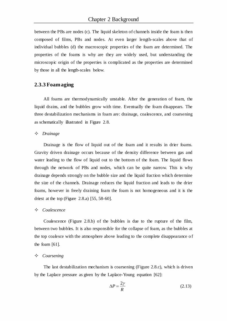
2.3.3 Foam aging
All foams are thermodynamically unstable. After the generation of foam, the
liquid drains, and the bubbles grow with time. Eventually the foam disappears. The
three destabilization mechanisms in foam are: drainage, coalescence, and coarsening
as schematically illustrated in Figure 2.8.
Drainage
Drainage is the flow of liquid out of the foam and it results in drier foams.
Gravity driven drainage occurs because of the density difference between gas and
water leading to the flow of liquid out to the bottom of the foam. The liquid flows
through the network of PBs and nodes, which can be quite narrow. This is why
drainage depends strongly on the bubble size and the liquid fraction which determine
the size of the channels. Drainage reduces the liquid fraction and leads to the drier
foams, however in freely draining foam the foam is not homogeneous and it is the
driest at the top (Figure 2.8.a) [55, 58-60].
Coalescence
Coalescence (Figure 2.8.b) of the bubbles is due to the rupture of the film,
between two bubbles. It is also responsible for the collapse of foam, as the bubbles at
the top coalesce with the atmosphere above leading to the complete disappearance o f
the foam [61].
Coarsening
The last destabilization mechanism is coarsening (Figure 2.8.c), which is driven
by the Laplace pressure as given by the Laplace-Young equation [62]:
2 P
R
(2.13)

Chapter 2 Background
where R is the bubble’s principle radius of curvature.
Figure 2.8 Schematic drawing of the three main foam destabilization mechanisms. (a) is drainage
of the liquid due to gravity, (b) Coalescence of two bubbles, (c) Coarsening of the bubbles due to
the Laplace pressure.
The gas pressure inside small bubbles is larger than inside large ones due to the
curvature of the bubble surface. As a consequence, the gas diffuses through the
aqueous films from the small towards the large bubbles leading to the disappearance
of the smaller bubbles [63]. In this way, the bubbles disappear one after another and
the remaining average bubble size increased.
2.3.4 Slowing down the ageing of foam
As discussed above, foams are thermodynamically unstable, although some
surfactants are very efficient in slowing down the ageing mechanisms. In order to
obtain very long lived (or ultrastable) foams, we need to find ways to radically slow
down or even stop the mechanisms that destabilize the foams.
The simplest way to slow down drainage is to increase the fluid viscosity. For
instance, adding some glycerol in the liquid phase leads to an increase of the bulk
viscosity which leads to a decrease of the drainage rate [64]. However, this will never
arrest the drainage. It will just be slowed down. In order to arrest drainage, the
continuous phase has to be either solidified (to have a yield stress) or larger particles
need to be trapped inside the channels to stop the channels from becoming smaller
and therefore to stop the drainage. It has been shown that drainage can be arrested

Chapter 2 Background
using a colloidal gel (made of Laponite), as the yield stress of the gel becomes higher
than the gravitational stresses driving the drainage of the foam [65].
In coarsening, the diffusion of gas through the liquid phase is the key step in the
in the process. Therefore using a gas which is poorly soluble or insoluble in the liquid
will slow down the gas transport through the liquid phase. Therefore, foam stability is
higher in the presence of fluorinated gases than nitrogen or air because their solubility
is much lower in water. However, this again does not stop the coarsening completely.
In order to stop coarsening, theoretical and numerical studies on the dissolution
of a single bubble have shown that either interfacial elasticity can arrest the foam
coarsening when the Gibbs stability criteria is satisfied:
Ed > σ/2 (2.14)
Or the foam coarsening can be arrested through making the bulk elastic enough [66].
2.4 Hofmeister series
All salts are not equal, the first person to classify them according to their ability
to salt out or salt in proteins was Franz Hofmeister after who the series of salts is
named. According to their ability to precipitate proteins, the order of cations is usually
given as follows:
N(CH3)+ < NH4+< Cs+ < Rb+ < K+ < Na+ < Li+ < Mg2+ < Ca2+
The sequence indicates that the negatively charged proteins remain stable in the
presence of high concentration of electrolyte containing the ions on the right side,
while they already precipitate at low concentration of electrolyte containing the ions
on the left side. Although the first studies of Hofmeister effect was more than 100
years ago [67-69], the reasons behind the ordering in the Hofmeister series are still
under debate. In a colloidal system, over more than a half century the aggregation
behavior of colloidal particles has been explained quite well with the DLVO theory.
However, as has been discussed in 2.2.1 the CCC predicted by the theory is the
same for all the monovalent electrolytes, which is not correct. It can’t explain the ion
specific effects on the particle aggregation within the Hofmeister series, since it
assumes that the ions have no difference except in their valence. In order to solve this

Chapter 2 Background
problem, one of the approaches is based on Collins’s concept of matching water
affinities [70]. Depending on how the ions interact with water, they can be divided
into two main groups: Kosmotropes and chaotropes as given in Figure 2.9.
Kosmotropes have a large hydration shell around the ion and experience a repulsive
dispersion potential with the surface. In contrast, chaotropes have a poor hydration
shell around the ion and experience an attractive dispersion potential [71].
Figure 2.9 The Groups of IA alkali cations and VIIA halide anions are divided into kosmotrope
(strongly hydrated) and chaotropes (weakly hydrated) according to their size [70]. The ions are
drawn approximately to scale of their bare radii.
2.4.1 Ions at interface
Although the properties of bulk electrolyte solutions can be described by the
theory of Debye and Hückel (DH) [72], the surface properties of electrolytes remain a
puzzle. The mystery first appeared when the surface tension of various electrolytes
was measured by Heydweiller [73] and it was observed that it is larger than the
interfacial tension of pure water. Recently theory and experiments have given new
insight into this problem. By using only one adjustable parameter-the hydrated radius
of sodium cation, ah=2.5 Å, Levin et al. [74] presented a new theory which can
explicitly calculate the surface tension, the ionic density profiles, and the electrostatic
potential difference across the solution-air interface. Predictions of the theory are
found to be in excellent agreement with the experiments. Schelero et al. [75-78]
investigated salt effects on the film thickness and stability of wetting films. They
found that with increasing the ion size (decreasing charge density), both cations and
anions show a stronger tendency to adsorb at the interface. The results demonstrate
that the effect of the hydration shell of ions dominates over electrostatics on their
adsorption at the air-water interface.

Chapter 2 Background
Except the air-water interface, the ions are absorbed on the surfaces of the
colloidal particles screening the electrostatic interactions and leading to the
aggregation of the colloidal particles [38-40, 79-81]. Oncsik et al. showed that the
differences in the aggregation rates in the presence of different types of salts could be
rationalized by taking into account the changing surface charge with the varying ion
adsorption [82], poorly hydrated counterions absorb strong on the surface of
hydrophobic latex particles and well hydrated counterions adsorb weakly or not at all.
2.4.2 Interactions between colloidal particles in the presence
of electrolyte
The interactions between colloidal particles in aqueous electrolytes solut ion are
relevant to fields ranging from molecular biology and bioengineering to the
colloidal-based technologies. As we discussed above, for more than half century, their
interactions are explained by the famous DLVO theory [83, 84], which is a very
successful theory can reproduce many phenomena. However, specific ion effects are
not taken into account in this theory.
Over the past 20 years, there has been a growing realization the importance of ionic
polarizability (the effective rigidity of the electronic charge distribution), which play a
significantly role in the ion specificity [85-88]. Ninham et al. [37, 89, 90] developed a
more analytical approach to ion specificity published a series papers over the past
decade and a half. They proved that the proper inclusion of quantum mechanical
non-electrostatic dispersion interactions missing from the classical theories of
electrolytes can explain ion specific effect at surfaces and in colloidal suspensions.
The London-Lifshitz theory predicts that the dispersion interaction between a surface
and an ion decays with the third power of separation and is proportional to the ionic
polarizability [91]. The chaotropic ions (K+, Cs+) have an attractive dispersion
potential with the micelle surface and the kosmotropic ions (Li+, Na+) have a
repulsive dispersion potential [71]. Force measurements between silica surfaces in
electrolyte solutions have given results consistent with the above theory. Taking ions
at the same concentration, more chaotropic ions adsorbed onto the silica surfaces
leading to a smaller force between the silica surfaces compared with the kosmotropic
ions. Moreover, as the ion concentration is increased more cations absorb to the
negatively charged silica surface and neutralize the surface charge, leading to
screening the electrostatic repulsion to reveal the Van der Waals attraction. However,

Chapter 2 Background
the concentration needed to neutralize the surface is not the same for different cations,
and it decreases as the cation radius increase. At even higher salt concentrations,
repulsion reemerges due to the surface charge reversal by excess adsorbed cations
[92]. Oncsik et al [82] also show that the ions of SCN- adsorption on positively
charges particles leads to charge reversal. Therefore, we can see that the ions with
same valence but different radius have different ability to aggregate particles.

Chapter 3 Materials and Methods
Chapter 3 Materials and methods
3.1 Materials
3.1.1 Phase separation
Succinonitrile (SCN, ≥99.9 %) was purchased from J&K and used without
further purification. Milli-Q water (18.2 MΩcm) was used to prepare the samples.
Iron(Fe, ≥99.99 % ) and tin(Sn, ≥99.999 %) were purchased from Alfa Aesar. Argon
(Ar) was used to eject the melted alloy to form ribbons. The mixture of HNO3 and
alcohol was used to etch the samples.
3.1.2 Gels
Silica particles (Ludox TMA from Sigma Aldrich (TMA in the following)) with a
particle diameter of 27 nm (from SAXS measurements) and a stock concentration of
34 wt% were used. The pH of the stock solution measured was 7.0. Sodium chloride
(NaCl, ≥99.5 %), potassium chloride (KCl, ≥99.0 %), lithium chloride (LiCl, ≥99 %),

Chapter 3 Materials and Methods
cesium chloride (CsCl, ≥99.9 %) and magnesium chloride (MgCl2, ≥ 99.9 %) were all
from Sigma Aldrich and were used without further purification.
In the light transmission experiments, same silica particles were bought from the
above company, but the pH is around 4, so the pH was changed to 7 by the addition of
NaOH.
Milli-Q water (18.2 MΩcm) was used for the preparation of all the samples.
3.1.3 Foam
Sodium dodecyl sulfate (SDS, ≥99.0 %) was purchased from Sigma Aldrich and
used without further purification. Sodium chloride (NaCl) and potassium chloride
(KCl) were the same as in gel. Milli-Q water (18.2 MΩcm) and D2O were used for the
preparation of aqueous solutions. Air was used as gas for most of the experiments and
perfluorohexane C6F14 was added for the SANS experiments to slow down foam
coarsening. Stock solutions of 1 M NaCl, 1 M KCl and 555 mM SDS were used in the
sample preparations. Due to the hydrolysis of the SDS the surfactant stock solution
was used within a week of preparation.
3.1.4 Gel foam
Sodium dodecyl sulfate (SDS) and sodium chloride (NaCl) were the same as in
the foam. Silica particles were brought from the same company Sigma Aldrich as in
the gel and have the same diameter with pH around 4. In all the related experiments,
we change the pH of the silica to 8 by using NaOH to make the particles less charged
and for the gel to form faster. Perfluorohexane C6F14 was used as gas to slow down
the foam aging. Stock solutions of 4 M NaCl and 555 mM SDS were used in the
sample preparations. The stock SDS solution was used within a week of preparation
to avoid the hydrolysis of SDS.

Chapter 3 Materials and Methods
3.2 Methods
3.2.1 Sample preparation in miscibility gap and calculation
3.2.1.1 SCN-H2O system sample preparation
SCN was added to the water solution and heated to 353 K for 20 min, then the
samples were immediately injected into the sandwiched cells with a dimension of 25
10 0.5 mm and sealed. The cell’s covers are made of glass and its height was
controlled by the Teflon film spacers. During the experiment, a round copper block
was used for producing an isothermal field and its temperature was controlled by the
3504 Eurotherm. The isothermal field was used for the micro phase separation of
nucleation growth (NG) and spinodal decomposition (SD) and observed by the optical
microscope. Two copper blocks with 10 or 12 mm distance were used for producing a
uni-directional thermal gradient and their temperature was controlled by the flow
inside the copper blocks. The uni-directional thermal gradient was used for the macro
phase separation of NG and SD simultaneously (the samples were put side by side or
separated) and observed by a Samsung camera. The samples were immiscible at room
temperature, and they were put in copper block at 353 K for 5 min before put in the
copper block for observation.
3.2.1.2 Fe-Sn ribbons preparation
The Fe-Sn alloys were melted by radio-frequency (RF) induction heating and
overheated to about 100 K above its liquidus temperature for several minutes under an
argon atmosphere in a 13 mm ID 15 mm OD 160 mm fused silica tube. The
overheated samples were ejected by Ar atmosphere with an overpressure of 50 kPa
through a nozzle (=0.7 mm) at the bottom of the silica tube onto a Cu single roller.
The wheel speed was set as 3 or 10 m/s.
Then the Fe-Sn ribbons were mounted in epoxy, sectioned, polished, and etched
with a mixture of 3 mL HNO3 + 100 mL alcohol. The solidification microstructures
were examined by Zeiss MAT optical microscope and TESCAN VEGA3 LMH
scanning electron microscopy (SEM). The chemical compositions of the identified
constituent phases were determined with an energy dispersive spectrometer (EDS)
fitted in SEM.

Chapter 3 Materials and Methods
3.2.1.3 Calculation of the spinodal curve and volume fraction
According to the theories of the thermodynamics, the spinodal curve is
calculated under the condition, 022 xG , for given temperatures, in which G
is the difference in Gibbs free energy during phase transformation, and x is
concentration.
On the basis of the thermodynamic theories, G can be expressed as [93]
n
k
k
jiji
k
i ij
jii
i
i xxLxxxxRTG0
,ln (3.1)
where R is the gas constant, T the temperature, xi and xj denote the
concentrations of pure substances i and j, ji
k L , is the kth binary interaction
parameter between i and j and may dependent on the temperature as A+BT,
in which A and B are model parameters.
For SCN-H2O system, ji
k L , s are given as follows (k = 0, 1, 2, 3) [94]
2
0 19240 44.85SCN,H OL T
2
1 9871 25.32SCN,H OL T
2
2 9412 25.52SCN,H OL T
2
3 19181 60.85SCN,H OL T (3.2)
For Fe-Sn system, ji
k L , s are given as follows (k = 0) [95]
12.818T+66760 Fe,SnL (3.3)
The spinodal curves of the SCN-H2O and Fe-Sn systems are calculated on the
basis of the above equations.
3.2.1.4 Calculation of the volume fraction
The density of SCN is 0.985g/cm3, which is close to the density of water 1 g/cm3.
So the volume fraction is close to the mass fraction in the phase diagram. The
schematic phase diagram in the miscible gap is shown in Figure 3.1. When the
temperature is quenched to T, a sample with composition C separates to two phases
L1 and L2, the corresponding concentration were C1and C2. We use the lever rule to

Chapter 3 Materials and Methods
calculate the volume fraction, the volume fraction of L1 is 1
2
2 1
L
C Cf
C C and
2 11L Lf f . TM is the bottom temperature of the miscibility gap.
Figure 3.1 Schematic phase diagram in the miscible gap.
3.2.2 Gel sample preparation and measurements
3.2.2.1 Gel sample preparation and rheology measurement
Silica stock was added to salt solutions ranging from 0-500 mM in concentration
and immediately agitated with a vortex mixer for 10 s to ensure homogeneous mixing.
Samples were then sealed to avoid solvent evaporation and stored for observation -
save for those samples prepared for SAXS and rheological experiments. These were
immediately transferred into SAXS capillaries (see below) and into folded paper
containers respectively, both of which were sealed and stored until the measurements.
The paper containers allowed transfer of the samples into the rheometer with minimal
perturbation.
After the gels go from liquid to solid, there are several two ways to measure how
their mechanical properties evolve. One way is to measure G’ and G’’ at different time
after gelation by using small amplitude oscillations (fixed frequency of 10 Hz and
strain 1 %), another way is to measure G’ and G’’ a t fixed time by using the strain
sweep measurement (at constant strain rate amplitudes 5s-1, where the strain is from
0.05 to 25). The former is to obtain the mechanical properties evolution with time
without destroying the structure of gel and the latter is to acquire the mechanical
properties evolution with strain at breaking the gel structure. From these

Chapter 3 Materials and Methods
measurements, we can know how the gel ages with time its yield strain.
3.2.2.2 SAXS measurements
The SAXS measurements were performed at the European Synchrotron
Radiation Facility (ESRF, Grenoble, France) on the bending magnet beamline BM02
(D2AM), at a photon energy of 7 keV. The experimental setup is described in detail in
reference [96]. The data were acquired using a CCD Peltier-cooled camera
(SCX90-1300, from Princeton Instruments Inc., New Jersey, USA) with a resolution
of 1340 × 1300 pixels. Data preprocessing (dark current subtraction, flat field
correction, radial regrouping and normalization) was performed using the bm2img
software developed at the beamline.
The samples were contained in cylindrical glass capillaries (Mark-Rörchen)
1 mm in diameter and the exposure times were between 2 and 10 seconds, depending
on the concentration. The samples which phase separate were measured in the lower
solid-like phase.
3.2.2.3 Modeling SAXS data
The intensity scattered by the spherical silica colloids can always be written as:
I(q)= ∆ρ2×n×S(q)×P(q) (3.4)
where S(q) is the effective structure factor, P(q) is the form factor of individual
colloids which is a constant characteristic of the system, ∆ρ is the electronic contrast
of the colloids and n is the colloidal density.
The form factor, P(q), in the case of spherical silica colloids is [97]:
P(q)=|F(q,R)|2= |3×sin(qR)-qR× cos(qR)
(qR)3 |2
(3.5)
where F(q,R) is the scattering amplitude of a sphere of radius R.
Experimentally, the form factor (in fact ∆ρ2×n×P(q)) can be evaluated in two
ways: i) from the scattered intensity I(q) of dilute solutions with high salt
concentration (where the electrostatic interaction is screened, and the structure factor
can be considered equal to 4); ii) from adjusting the scattering intensity I(q) at high
q-values from various individual curves; a method allowing to estimate the uncertainty
on and the effective values of ∆ρ2×n.

Chapter 3 Materials and Methods
The effective structure factor is then obtained for each image as:
S(q)=I(q)
∆ρ2×n×P(q)
(3.6)
During the formation of gels, S(q) becomes time-dependent (since I(q) is also
time-dependent due to the clustering of the colloids) and is composed of two different
contributions: i) the contribution of the effective interactions between individual
colloids inside the clusters; ii) the contribution of the cluster dimension. The first
contribution arises at intermediate q-values while the second is at low q-values. In the
case of mass fractal gels (as expected at the lowest volume fractions), the latter is
characterized by an increase in forward scattering corresponding to the dependence of
the signal as q-Df where Df is the fractal dimension [44, 45]. However, our
experiments probe mainly the local colloidal environment due to the q-range
accessible (the lowest q-value is around 4 × 10⁻³ Å-1
). In addition most of our
experiments are at relatively high silica volume fractions where the experimental
determination of the fractal dimension from the S(q) is not direct [98]. As a
consequence, we use a simple model, where the contribution of the cluster inner
structure is taken as a constant baseline, B, to which a power law is added, resulting in
Aq-α+B. This has been applied for q<0.01Å-1
on the data once the S(q) have
stopped evolving to obtain . We use the power exponent to compare the results at
different volume fractions.
3.2.2.4 Light transmission observation for gels
Gel samples were prepared the same way as in 3.2.5. After the gel samples were
prepared, they were transfer to a black box, light source was provided by the white
light. Images were taken by a UEye camera every 5 minutes. Before starting to
observe, a black cloth was covered on the black box to avoid environment light to
influence the experiments.
3.2.3 Foam sample preparation and stability studies
3.2.3.1 Preparing KDS
KDS was obtained from SDS by an ion exchange in KCl solution [99]. SDS
powder was dissolved in KCl solution (1M) at 50 °C up to a ratio of the components

Chapter 3 Materials and Methods
of KCl:SDS = 2:1. Then the solution was allowed to stand at 50 °C for 2 h and at
room temperature for next 12 h [99]. The sediment was filtered out using a Shott filter,
washed with Milli-Q water and acetone and dried in air until the mass remained
constant. The product yield was about 95%.
3.2.3.2 Determination of the dissolution temperature and kinetics of
crystal formation
The samples were crystallized by cooling them below the dissolution
temperature. The temperature was slowly increased by 1 ℃ every 30 minutes. Once
the crystals started to dissolve this was slowed down to 0.5 ℃ every 30 minutes. The
dissolution temperature was defined as the temperature when the crystals became
invisible to the eyes. Then the samples were placed in a water bath heated 1 ℃
higher than the measured dissolution temperature above until no crystals can be
observed. The temperature was then set to the target temperature at which the sample
was observed and the time at which crystals started appearing was noted as the
crystallization time.
3.2.3.3 Making foam
All the foams were prepared at room temperature (T=21±2℃), unless otherwise
stated in the text. The foams were prepared using a setup consisting of two disposable
syringes connected by a constriction. The volume of a syringe is 20 mL and the
diameter of the constriction is 2 mm. The syringes are filled with air (with some C6F14
for the SANS experiment) and foaming solution. Salt solution and water start in one
syringe, and the SDS solution in another. This ensures that they come into contact
only as the foam generation process begins. Different ratios of liquid to gas were used
to make the foams, most often 1:4 or 1:8, and the total volume of foam made was
varied. The foam is formed by pushing the liquid and gas forward and backward
through the constriction 40 times.
3.2.3.4 Foam stability studies
After making the foam, the samples were transferred into glass vials. Images
were taken by a UEye camera every 5 minutes at room temperature and at varying
intervals when heated (according to the foam disappearance rate). Some of the
samples were photographed under a microscope to observe the bubble surfaces more

Chapter 3 Materials and Methods
closely. For the heated samples, the temperature was set above the previously
measured precipitation temperature, using the microscope to observe the micro
evolution of the foam bubbles and a UEye camera to obtain the foam’s macro
evolution.
3.2.3.5 Small angle neutron scattering experiments
The experiments were carried out at the Orphée reactor in Saclay on the PAXY
spectrometer. Three different configurations were used with wavelengths of λ = 15 Å
and λ = 4 Å and sample to detector distances of 6.75 m and 1.250 m. This gives an
accessible scattering vector q-range from 2 × 10⁻³ to 5 × 10⁻¹ Å-1. Samples were
enclosed in quartz cells of 1 mm inner thickness with pure D2O as solvent. All the
measurements were performed at atmospheric pressure and room temperature. The
scattered intensities were corrected for the detector background by cadmium
scattering, for the parasitic intensity scattered by quartz cell and empty beam by
subtraction and normalized to the water scattered intensity. Standard procedures for
data reduction [100] were done using the Pasinet software [101]. Absolute values of
the scattering intensity, I(Q)in cm-1, were obtained from the direct determination of
the number of neutrons in the incident beam and the detector cell solid angle [102].
The scattering intensity of the solute was obtained by subtraction of the intensity of
the solvent (measured independently) to the one of the solution. In the following, this
final intensity will be noted I(q).
At high q (> 0.2 Å-1) the intensity saturates to a constant value for both samples
due to the incoherent scattering. The intensity of the sample with KCl is higher,
because the foam prepared with potassium is more stable and there is more sample.
The foam made with NaCl the foam partially collapsed during the experiment.
3.2.3.6 Calculating the enthalpies of dissolution of NaDS and KDS
The equilibria between crystals and micelles are set by kinetic constants, which
depend on the concentrations of the constituents. These kinetic constants can be
linked to the change in Gibbs free energy as ∆G0= -RTlnK= ∆H0-T∆S and a Van’t
Hoff plot will allow us to estimate the enthalpies of dissolution from
ln K= -∆H
RT+
∆S
R (3.7)

Chapter 3 Materials and Methods
In order to calculate this we need to take several approximations. We assume that
the concentration of monomers is negligible (reasonable as we are working with 69
mM DS- and the CMC of SDS is below 1mM at the salt concentrations studied [103]).
We also assume that the micellar size is sufficiently peaked that we consider only one
size of micelle, which does not depend on the salt concentration. We also assume that
the counter ion binding does not depend on the bulk salt concentration, and we
assume them to be the same and constant value of 0.8 for both salts (the degree of
binding has been shown to depend little on temperature [104]).
The case with SDS with the added KCl is much more complicated due to the
presence of both Na+ and K+. This is why for both salts we only consider the range of
high added salt concentrations (from 0.5 to 1 M). This means that the added salt
concentration is much higher than that of the SDS and for the analysis with KCl we can
neglect the concentration of sodium ions. The absolute values of H change if we
change the range, however we always find HSDS lower than HKDS. This is why we
only discuss the difference between the H and not the absolute values.
Dissolution of NaDS
Where n is the number of Na+ associated with a NaDS micelle and m is the
number of monomers per micelle (aggregation number). The melting process can be
written as:
m
(m-n)NaDS
K1↔Na++
1
m-nNa
n
DSm(n-m) (3.8)
Below the melting temperature all of the SDS is in the micelles, so the number of
micelles is CSDS/m and [DS-]≈0 and the concentration of sodium ions can be written
as[Na+]=cNa-n[NanDSm]≈cNa-βcSDS
, where for Na+ the total concentration of sodium
includes the counter ions from the SDS molecules as well as the added salt and is the
degree of counter ion binding onto the micelles.
We can describe the reaction coefficient in terms of the known concentrations as:
K2=(CNa-βCSDS)∙(CSDS
m)
1
m-n. In Figure 3.2 we show the plot of lnK2 as a function of 1/T.
Assuming a constant enthalpy and entropy, which is not unreasonable considering the
linearity of the data, we can get the enthalpy of dissociation of SDS as 75 kJ/mol.

Chapter 3 Materials and Methods
Dissolution of KDS
Thus corresponding equation for melting (with constant K4) can be exactly
analogously to those of SDS. The reaction constant of melting can be simply written as
K4=(cK- βcDS)(CKDS
m)
1
m-n. In Figure 3.2 we also show a plot of lnK4 as a function of 1/T.
This allows us to extract the enthalpy of dissolution of KDS as 88 kJ/mol.
Figure 3.2 The Van’t Hoff representations of the SDS and KDS melting temperatures. The lines
are linear fits and the slopes are used to calculate the enthalpies of dissolution.
3.2.4 Foam aging with gel phase
3.2.4.1 The way to change pH of the TMA solution
2M NaOH solution was prepared first. Then a certain volume of TMA solution
was taken from the bulk solution and put in the glass vial. The solution was stirred
using a magnetic stirrer and NaOH solution was added little by little while the pH of
the solution was measured. The addition was stopped when the pH of the solution
reached 8, at which point the amount of NaOH solution used was noted. For the
following solutions the same amount of NaOH was added to the same quantity of
TMA solution without measuring the pH again. We considered the pH obtained is 8.
However, each time when change the volume of TMA solution, the process to
measure how much NaOH solution needed to get pH=8 was repeated again.

Chapter 3 Materials and Methods
3.2.4.2 Making gel foam
All the foams were prepared at room temperature (T=21±2 ℃) and generated by
the foam machine connected with two syringes at velocity 50mm/s and 20 times. The
volume of a syringe is 60 mL and the diameter of the constriction is 2 mm. The
syringes are filled with air saturated with C6F14 and foaming solution. Salt solution
and water are put in one syringe, and the SDS solution and TMA solution in another.
This ensures that they come into contract only as the foam generation process begins.
The ratio of liquid to gas was 1:6 and the total volume of liquid was 7 mL.
3.2.4.3 Gel foam studies
After making the gel foam, the samples were transferred into petri dishes, which
were fixed with clips and at set vertically. A rectangular prism was put in the center of
the cell to take high resolution photographs of the surface of the gel foam. Images
were taken by a UEye camera every 5 minutes at room temperature.
3.2.4.4 Rheology studies in the bulk gel phase
In order to compare the gel phase evolved in the gel foam, bulk gel rheology was
measured using a rheometer. SDS solution, TMA solution, salt solution and water
were mixed without making foam and transferred into the double gap of rheometer
immediately. We waited for 1 hour and started to measure the storage (G’) and loss
moduli (G’’) at a fixed frequency of 1 Hz and strain 1 %. The measurements
continued for three hours, stopped and waited for 20 min, then started again to
measure G’ and G’’ at fixed frequency of 1 Hz and varied strain from 0.01 to 500 %.

Chapter 4 Phase separation mechanisms studied in miscibility gap
Chapter 4 Phase separation mechanisms
studied in miscibility gap
4.1 Introduction
In nature, a phase transition proceeds spontaneously if the total free energy of a
system decreases, or proceeds along the direction to a low chemical potential. This
leads to two manners of phase separation in the system with a miscibility gap:
nucleation-growth (NG in the following) and spinodal decomposition (SD in the
following) [105, 106]. The miscibility gap, exists in a considerable number of
different systems such as fluid mixtures [107-110], polymer mixtures [7, 8], glasses
and ceramics [111, 112], and metallic systems [113-115], so the NG and SD processes
occur frequently in daily life. For this reason, the understanding of the mechanisms on
the phase separation via the two manners is essential in the areas of condensed matter
physics, materials science, and biological sciences.
From the point of view of variation in the free energy, the NG-type phase
separation is a metastable process and tiny perturbations leads to an increase in free
energy. The free energy can only be decreased in the case if nuclei are formed with a
composition very different from the matrix. While the SD-type one is an unstable

Chapter 4 Phase separation mechanisms studied in miscibility gap
process. Small perturbations will cause the free energy to decrease and therefore it
proceeds spontaneously. From the point of view of the morphology evolution, the new
phase formed in NG process is well separated droplet. Whereas in SD process the new
phase forms in two stages: in the early stage, long-wavelength delocalized
concentration fluctuations grow exponentially and interconnected domains or network
like structures are produced. Then in the later stage, the interconnected domains
coagulate and evolve into droplets. The characteristic droplets radius r grows with
time as mr ~ t , where m = 1/3 in the early, purely diffusive stage, and m = 1 at a
later time, when the surface tension effects become dominate [116, 117]. In the later
stage, the growth of the new phase droplets via the SD manner is like that of
nucleation [118-120]. This is the reason why the researchers in the field of condensed
matter physics usually believed that there is no significant difference between NG and
SD [121]. However, due to the difference in the early dynamic processes of the two
manners and their volume fraction of the minority phase, the pattern evolutions may
be changed drastically if some external conditions are imposed.
In this study, NG and SD type phase separation were realized in a transparent
system, SCN-H2O, which has a miscibility gap. The reason to select the transparent
system is that their phase separation process can be observed in-stiu. Otherwise, for
the alloy system, their phase separation process only can be inferred from their final
structure. Temperature and isothermal field were imposed on the samples with these
two types phase separation. It was found that the pattern formations via these two
manners are quite different. The evidences obtained in the present work show that the
NG and SD type manners will result in distinct morphology evolutions which could
have potential applications in designing specific structural materials.
4.2 Results and discussion
4.2.1 Phase separation of SCN-H2O system in a
uni-directional temperature field
Phase diagram of SCN-H2O system is shown in Figure 4.1. NG and SD type
phase separation can be obtained according to the phase diagram. In this experiment,
SCN-70wt%H2O and SCN-50wt%H2O were chosen to realize the process of NG and
SD in the uni-directional temperature field. The macroscopic NG and SD type phase

Chapter 4 Phase separation mechanisms studied in miscibility gap
separation processes were investigated simultaneously in the temperature field at low
temperature (left side) TL=297.5 K and high temperature (right side) TH=330.5 K. The
photographs as they evolve in time were shown in Figure 4.2. Photographs of NG
process with SCN-70wt%H2O solution was given in (a) and SD process with
SCN-50wt%H2O solution was given in (b).
Figure 4.1 Phase diagram of SCN-H2O system [115]. Metastable and unstable regions were
divided in the miscibility gap. In the former, the phase separation type was NG (between the
binodal and spinodal line in the immiscible gap), whereas in the latter the phase separation type
was SD (below the spinodal line).
As shown in Figure 4.2, the phase separation of NG and SD processes both
started at the low temperature side, this is because the sample at low temperature side
will go into the miscibility gap first. However, the macroscopic morphology evolution
of the two types of phase separation was distinct.
The NG type, SCN-rich phase which has a small volume fraction and defined as
the minority phase, nucleated as droplets in the matrix after the temperature is
quenched below the binodal line. In Figure 4.2(a) at 4 s, most of the solution was still
miscible, then at 10 s it can be seen that there were many droplets formed and pushed
to the high temperature side by the Marangoni force [122, 123], which was caused by
the interfacial tension gradient between a spherical droplet and a liquid matrix [15].
After the droplets formed, they can surpass the interaction interface front as they
migrated to the high temperature side like at 20 s. This was much more obvious at 30
s and the size of the droplets became larger during the migration. One can note that

Chapter 4 Phase separation mechanisms studied in miscibility gap
there were still many droplets and no apparent aggregation was observed.
Figure 4.2 Macroscopic morphology evolution of NG with SCN-70wt%H2O solution (a), and SD
with SCN-50wt%H2O solution (b) with time. The low temperature (left side) was TL=297.5 K and
high temperature (right side) TH=330.5 K. The red dash line in (b) was the interfacial layer
between the matrix phase and the minority rich phase.
Nevertheless, the SD type, the morphology evolution was totally different. At the
time of 4 s (the time t=0 is when SD type phase separation started) as shown in Figure
4.2(b) phase separation had occurred, this is because the spinodal temperature for
SCN-50wt%H2O is higher than the binodal temperature for SCN-70wt%H2O. After
the SD type phase separation started, big size aggregations formed very soon as seen
clearly in Figure 4.2(b) at 10 s. Then from the macroscopic perspective, there was one
large aggregate formed which continued to grow as it migrated to the high
temperature side pushed by Marangoni force, but there were many small droplets
inside it. They formed one large aggregate in order to decrease the interfacial energy
when the migration process proceeds. The newly produced droplets continued to
merge into the large aggregate, which is why it continued to grow.
During this process, one obvious interfacial layer formed marked as the red dash
line like at 20 s. The interfacial layer was not straight due to contact with the edges of
the sample. In fact, the interfacial layer was the left side of the large aggregate and
migrated to the high temperature side together with it. The front of the large aggregate
was cellular as a result of the instability of it.

Chapter 4 Phase separation mechanisms studied in miscibility gap
In order to have a better understanding of the difference between the two types of
phase separation we take a closer look at the samples. Figure 4.3 gives the
microscopic evolution of NG type phase separation for SCN-70wt%H2O at different
times observed by the microscope under the uni-directional temperature field. The left
side (low temperature) was 297.5 K and right side (high temperature) was 323.5 K.
Figure 4.3 Photographs of the phase separation of NG for SCN-70wt%H2O evolution in time
observed by microscope under the uni-directional temperature field. The low temperature (left side)
was TL=297.5 K and high temperature (right side) TH=323.5 K.
The microscopic phase separation was similar like in the macroscopic process.
The SCN-rich phase nucleated as small droplets in the matrix when the temperature
below the binodal temperature and the droplets migrated to the high temperature side
pushed by the Marangoni force. In the beginning, the droplets were too small to be
seen clearly. This is because the lens we selected is small and the purpose is to
compare the microscopic phenomenon with the macroscopic one. The droplets can be
seen clearly as they evolve during 20 s. One can note that the small droplets grow
larger and larger along with their migration and the velocity of bigger droplets was
faster than the smaller one, which can be seen in Figure 4.3 at 20 s that the droplets
with lager radius at the right side of the photograph.
For comparison, the evolution of SD type phase separation for SCN-50wt%H2O
at different times observed with the microscope under the uni-directional temperature
field was shown in Figure 4.4. The low temperature (left side) was 293 K and high
temperature (right side) was 333 K. The microscopic phase separation was similar as
in the macroscopic process as well. In the microscopic process, the aggregated of
droplets can be seen clearly. For the SD process, the initial transition of network-like

Chapter 4 Phase separation mechanisms studied in miscibility gap
structure to the spherical droplets was fast, especially under the temperature gradient,
so in the beginning of Figure 4.4 we only saw the small droplets instead of the
network- like structure. The small droplets are pushed by the Marangoni force and
they aggregate very fast like in the macroscopic process. One can note that at 6 s the
big size aggregates side by side have the trend to connect together. Then at 10 s they
connected to form one large aggregate and an obvious interfacial layer produced like
at 20 s in the macroscopic process. The small droplets on the left side of the layer
continue to merge into the large aggregation as the blue arrow pointed in Figure 4.4 at
10 s.
Figure 4.4 Images of microscopic phase separation of SD for SCN-50wt%H2O evolved as time
observed by the microscope under the uni-directional temperature f ield. The low temperature (left
side) was TL=293 K and high temperature (right side) TH=333 K. The red dash line was the
reaction interface front.
At 10 s, the layer is not formed in Figure 4.2 but it is already formed in Figure
4.4. Therefore, the speed to form the layer was faster in the microscopic than in the
macroscopic process. One reason was that the observed scale in microscopic process
was smaller compared with the macroscopic one. The second reason was that the left
side temperature was lower and the right side temperature was higher in the
microscopic process. When we did the experiment, there was another difference
between microscopic and macroscopic, the distance between low and high
temperature side was 12 mm in microscopic and 10 mm in macroscopic respectively.
Not like the NG type, the microscopic evolution of SD type phase separation was

Chapter 4 Phase separation mechanisms studied in miscibility gap
different as in the macroscopic process where only one interfacial layer formed. For
the microscopic process of SD type, the way to form the first layer during 10 s was
similar like in the macroscopic process. Nevertheless, as the phase separation
continued, when the velocity of reaction interface front was higher than the migration
of the aggregation front, the aggregation behavior of the minority phase would repeat
the process from 0 to 10 s and form another interfacial layer as shown in 50 s. The red
dash line was the reaction interface front, which partially surpassed the big aggregate
front at 19 s and totally surpassed it at 32 s. Then the formation process of the second
interfacial layer was like the first one. We didn’t see this in the macroscopic process.
May be because the sample is longer and the temperature interval between the low
and high side is larger in the microscopic process than in the macroscopic one. For
this experiment, the right side temperature was higher than the spinodal temperature,
so the second interfacial layer with the big aggregate would disappear as they
migrated to the position where the temperature was higher than the spinodal
temperature.
The radius of the drop is hard to measure during the migration when the
temperature gradient exists. In order to avoid this deficiency, next the NG and SD
types were performed at the temperature 1 K lower than binodal and spinodal value
under the condition with isothermal field.
4.2.2 Phase separation of SCN-H2O system at isothermal field
Figure 4.5 was the microscopic evolution of the phase separation process at
isothermal field observed by the microscope. Photographs of SCN-70wt%H2O
solution with NG type at T=323 K evolved as a function of time was shown in (a).
From the phase diagram of Figure 4.1, it can be known that the SCN-rich phase was
minority phase and nucleated as small droplets after the phase separation started.
Then the small droplets grow bigger and bigger with time, which is a typical
characteristic of the nucleation growth. All the droplets are separated from their
neighbors and they grow independently by pure diffusion without coalescence.
Photographs of SCN-50wt%H2O solution with SD type at T=330 K evolved in time
was shown in (b). The difference to the NG type is that the network- like structure
formed when the temperature quenched below the spinodal line for SD type as shown
in 3 s. The network- like structure is typical of the initial state of the spinodal

Chapter 4 Phase separation mechanisms studied in miscibility gap
decomposition growth and cannot be seen clearly under the condition of exerting the
temperature filed. Then the network- like structure coarsens and the shape becomes
spherical (as shown at 24 s), which is similar to that of nucleation. This process was
much faster in the uni-directional temperature since the droplets would collide and
merge with each other.
Figure 4.5 Microscopic evolution of the NG type phase separation at T=323 K with
SCN-70wt%H2O solution (a), and SD type at T=330 K with SCN-50wt%H2O solution.
Figure 4.6 Radius increased with time for both NG and SD type phase separation, three
droplets were chosen for each type measurement.
The relationship between the radius of droplets and time at isothermal field was
shown in Figure 4.6 for both NG and SD type phase separation. Three droplets for
each type were chosen for the measurements. We considered the time 0 s as we saw

Chapter 4 Phase separation mechanisms studied in miscibility gap
the spherical droplets or network- like structure appear by our eyes, this would have
some errors compared to the real case. For SD type, the measurement started after the
network- like structure transition to the spherical droplets. It can be seen that the
growth of the droplets via SD type was faster than the NG type and the relationships
of 0.636 2.612SDR t t and 21123.1 ttRNG were obtained, respectively. The
parabolic law 1 2( )
NGR t t is a typical characteristic of pure diffusive growth process
for NG case [124]. On the contrary, the linear law ( )SD
R t t is the typical
characteristic of the later stage of the spinodal decomposition when the surface
tension effects become dominant [125-127], the constant -2.612 comes from the time
0 we selected is not the real time 0. Therefore, we can see that the data in our
experiment agrees well with the theory of NG and SD type phase separation.
Moreover, it should be noted that when extend the fitted linear line of SD to the
X-axis, the radius of the minority phase for SD is negative at t=0. This is because that
the morphology of SD in the beginning is network like, however, the radius of the
minority phase is measured after its shape transformed from network like to spherical.
This means that it’s reasonable the radius of the minority phase is negative when
extend the fitted linear line of SD to the X-axis at small t.
Figure 4.7 Volume fraction of the SCN-rich phase as a function of temperature for
SCN-50wt%H2O (red solid line) and SCN-70wt%H2O (blue dash line).
The volume fraction of SCN-rich phase (the calculation method given in section
3.2.1.4) for samples SCN-50wt%H2O (SD type) and SCN-70wt%H2O (NG type)
evolution with temperature was shown in Figure 4.7. In both cases, the minority
phases were SCN-rich phase (fSCN). The red solid line was SCN-50wt%H2O and the

Chapter 4 Phase separation mechanisms studied in miscibility gap
blue dashed line was SCN-70wt%H2O. For SCN-50wt%H2O, fSCN was a little bit
smaller than 0.5 and constant for all the temperature, whereas for SCN-70wt%H2O, it
can be seen that fSCN near 0 when the temperature near the binodal temperature
(around 325 K) and increased to the maximum of 0.25 when the temperature
decreased to reach the bottom of the miscibility gap (around 290 K). The different
volume fractions of the minority phases can affect the aggregate behavior during the
phase separation process.
4.2.3 Growth rate and volume fraction of minority phase to the effect
of the microstructure
From Figure 4.2, it can be seen that the migration velocity and aggregation rate
of the minority phase in NG type are slower than in SD type after the phase separation
started. The migration of the minority phase droplets in the liquid matrix is induced
mainly by Marangoni motion and the velocity is given by [12, 128]
x
T
T
rv
md
m
233
2 (4.1)
where r is the radius of the droplet, d and m are the viscosities of the droplet and the
liquid matrix, is the interfacial energy, T is the temperature, and x is the distance.
Under the current experimental conditions, the two samples are put in the same
temperature field at the same time. This means that the temperature regimes are nearly
the same for both the NG and SD type phase separations, which results in almost the
same interfacial tension gradients and the viscosities. In this case, m is mainly
decided by and is proportional to r. Thus, the droplet radius plays a key role in the
migration.
The relationship between the radius of the minority phase and time under the
condition with isothermal field was shown in Figure 4.6, it can be seen that the radius
of the minority phase is proportional to t for SD type phase separation after transition
to the spherical droplets and proportional to t1/2 for NG type. This suggests that the
growth kinetics of the minority phase in SD is faster than in NG. As can be seen in
Figure 4.6, the droplets formed via the SD have a larger size than via the NG if the
phase separation starts at the same time. This makes the migration of the droplets
during the SD faster than during the NG process. Meanwhile, the higher growth rate
of the minority phase has higher possibility to aggregate. However, we should keep in
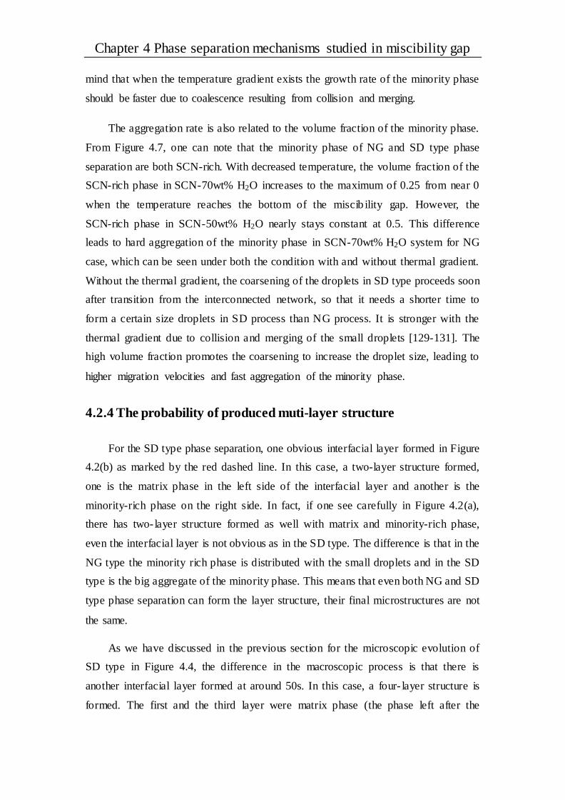
Chapter 4 Phase separation mechanisms studied in miscibility gap
mind that when the temperature gradient exists the growth rate of the minority phase
should be faster due to coalescence resulting from collision and merging.
The aggregation rate is also related to the volume fraction of the minority phase.
From Figure 4.7, one can note that the minority phase of NG and SD type phase
separation are both SCN-rich. With decreased temperature, the volume fraction of the
SCN-rich phase in SCN-70wt% H2O increases to the maximum of 0.25 from near 0
when the temperature reaches the bottom of the miscib ility gap. However, the
SCN-rich phase in SCN-50wt% H2O nearly stays constant at 0.5. This difference
leads to hard aggregation of the minority phase in SCN-70wt% H2O system for NG
case, which can be seen under both the condition with and without thermal gradient.
Without the thermal gradient, the coarsening of the droplets in SD type proceeds soon
after transition from the interconnected network, so that it needs a shorter time to
form a certain size droplets in SD process than NG process. It is stronger with the
thermal gradient due to collision and merging of the small droplets [129-131]. The
high volume fraction promotes the coarsening to increase the droplet size, leading to
higher migration velocities and fast aggregation of the minority phase.
4.2.4 The probability of produced muti-layer structure
For the SD type phase separation, one obvious interfacial layer formed in Figure
4.2(b) as marked by the red dashed line. In this case, a two-layer structure formed,
one is the matrix phase in the left side of the interfacial layer and another is the
minority-rich phase on the right side. In fact, if one see carefully in Figure 4.2(a),
there has two-layer structure formed as well with matrix and minority-rich phase,
even the interfacial layer is not obvious as in the SD type. The difference is that in the
NG type the minority rich phase is distributed with the small droplets and in the SD
type is the big aggregate of the minority phase. This means that even both NG and SD
type phase separation can form the layer structure, their final microstructures are not
the same.
As we have discussed in the previous section for the microscopic evolution of
SD type in Figure 4.4, the difference in the macroscopic process is that there is
another interfacial layer formed at around 50s. In this case, a four- layer structure is
formed. The first and the third layer were matrix phase (the phase left after the
Chapter 4 Phase separation mechanisms studied in miscibility gap
minority phase migrated) and the second and the fourth layer were the big aggregate
of the minority phase. The evolving process of the second layer interface is exactly
the same as the first layer interface formation process. In our case, finally the second
layer interface and the big aggregate will melt and disappear. This is because the
temperature at the high temperature side is higher than the spinodal value.
Considering that if the sample is long enough and can be moved and solidified
during its migration process, and the temperature controlled appropriately to keep the
temperature of the reaction interface front always lower than the spinodal value. Then
the aggregation process can be repeated and a multi- layer structure can be formed
with matrix and the big aggregate of the minority phase alternately.
According to the analysis above, multi- layer structure also can be formed in the
NG process. The mainly difference is that in the multi- layer structure, the minority
rich phase in SD process is the big aggregation and in NG process is the distribution
of the small droplets.
4.2.5 The phase separation pattern to the effect of the solidified
structure
The system of Fe-Sn alloy who has a miscibility gap. Next we will see what the
phase separation pattern to the influence of the solidified structure of Fe-Sn system.
The ribbons of Fe-Sn alloy [132] were prepared by ejecting the melted sample onto a
Cu single roller at certain wheel speed. The phase diagram of Fe-Sn alloy is given in
Figure 4.8(a), the red dashed line is the spinodal line. The solidification
microstructure of a ribbon at a wheel speed 10 m/s of Fe-68wt%Sn alloy is shown in
Figure 4.8(b), which experiences SD type phase separation. The dark phase in (b) is
Sn-rich phase and the light one is Fe-rich phase. The fibers of Fe-rich phase formed in
the upper side of the ribbon, this is the result of the aggregation of the minority phase
(Fe-rich), which is similar like the aggregation process of SD type in SCN-H2O
system. In the bottom of the ribbon, the typical initial fine network like structure of
SD type was preserved and (b’) was the enlargement of the area selected in (b). Such
structure can be preserved in the bottom of the sample since the cooling rate near the
wheel side is high and the initial SD morphology does not have time to coarsen before
solidifying totally.
From (b’), we can see that the influence of cooling rate to the final solidified

Chapter 4 Phase separation mechanisms studied in miscibility gap
morphology is very important. The network like structure was small in the bottom of
(b’) and much larger in the upper part. This is because the cooling rate near the wheel
side was the maximum and decreased toward the upper part of the ribbon. Like shown
in (b) the fibers of Fe-rich phase formed in the upper part of the ribbon, which has
smaller cooling rate, the Fe-rich phase has enough time to aggregate to form the fiber.
It should be noted that the structure shown in the upper part of (b) is a rudiment of the
layer structure since the cooling rate is high and the different small parts cannot
aggregate into the long layer. For comparison, the solidification microstructure via
NG type phase separation of Fe-58wt%Sn alloy at 3m/s is presented in Figure 4.8(c).
In this concentration, the minority phase is Sn-rich phase. As given in (c) that the
Sn-rich droplets nucleated and distributed homogeneously in the matrix and there is
no evidence to form fiber or layer structure.
Figure 4.8 (a) Phase diagram of Fe-Sn system. (b) SEM image of the SD-type solidif ication
microstructure in Fe-68wt%Sn alloy at 10 m/s. (b’) Enlargement of area in (b) selected to show
the worm-like structure. (c) The NG-type solidification microstructure in Fe-58wt%Sn alloy at 3
m/s. In the images, the dark phase is Fe-rich phase and the light one is Sn-rich phase.
In fact, for the alloy system with a miscibility gap, normally the temperature
interval is more than 1000 K, the cooling rate is extremely fast when the melted

Chapter 4 Phase separation mechanisms studied in miscibility gap
samples are quenched to room temperature. Like in the Fe-Sn ribbon, the cooling rate
is so fast that the initial phase separation morphology in the immiscib ility gap can be
reserved. However, a perfect layer structure needs good a design of the thermal
gradient and the cooling rate.
Although the late stage evolution of the minority phase in SD type is similar like
in NG type under the isothermal field, both are the spherical droplets as shown in
Figure 4.5. This is the reason why researchers in the field of condensed matter physics
usually believed that there is no significant difference between NG and SD during the
phase separation process [121]. However, if the morphology can be solidified in the
early stage of the phase separation process, the two processes should have a difference.
Figure 4.8 (b) and (c) are the Fe-Sn ribbon of SD and NG type. It can be seen clearly
that the network like structure in the early stage of SD type and the spherical droplets
in NG type phase separation are preserved. This proved that the different initial phase
separation pattern of NG and SD can lead to different morphologies. Even in the late
stage of SD, the formed morphology under the thermal gradient can have big
difference because of the different growth kinetics and volume fraction of the
minority phase in NG and SD, like the formed layer structure in SCN-H2O system.
Therefore, we can see that these two processes of phase separation can lead to
different morphologies.
4.3 Conclusions
In this study, SCN-50wt%H2O and SCN-70wt%H2O solution were used to
realize SD and NG type phase separations. Under the thermal gradient, macroscopic
observations show that the aggregation rate of the minority phase with SD type is
faster than NG type and two layer structures can be formed for both cases.
Nevertheless, the difference is that with SD type the second layer is the large
aggregates of the minority phase and with NG it’s the distribution of the minority
phase. For the microscopic observations, NG type is similar as in the macroscopic
case, but SD type can produce four layer structures and the formation process of two
latter layers is the repetition of the two former layers.
Under the isothermal field, the relationship of droplet’s radius and time shows
that the growth rate of the minority phase with SD type is faster than with NG type.
Compared with NG type, SD type has a higher volume fraction of the minority phase

Chapter 4 Phase separation mechanisms studied in miscibility gap
and it is easier to coagulate to form the big aggregates. This suggests that the kinetics
properties and the volume fraction of the minority phase play key role in the change
in the morphology evolution.
The results of Fe-Sn ribbons show that due to the initial distinct structure
characteristic of these two types of phase separation, different morphologies can be
obtained. In addition, multilayer structures can be produced if the thermal gradie nt
and the cooling rate can be well designed. However, although the late stage evolution
of minority phase in SD type is similar like in NG type, the formed multilayer
structures with minority rich phase are still not same, big aggregates and distribution
of minority phase respectively.
Thus, we can conclude that NG and SD type phase separation can produce
different morphologies. According to our findings, the materials can be designed by
selecting appropriate parameters to suit the specific material purposes.
Chapter 5 Influence of salt type on gelation kinetics (NaCl or KCl)
Chapter 5 Influence of salt type on gelation
kinetics (NaCl or KCl)
5.1 Introduction
Gels are important in many applications, such as in materials science, food
science, biological cells and so on [133-136]. Though gelation has been described in
several reviews [137-139] many aspects of this process are still not fully understood.
To make a gel, the building blocks identified above must aggregate. Aggregation can
be induced in a number of ways. For colloidal particles, for example, depletion
interactions arising from a polymer in solution can lead to gels that are the result of an
arrested phase separation[140, 141]. In many food systems, gels are the result of the
protein denaturation that precedes aggregation [142, 143]. In this case, the loss of
stability comes from the interactions between protein domains that are not exposed in
the native form[143].
As in most complex fluids, the repulsive electrostatic and the attractive van der
Waal forces play an important role in the stability of colloidal and nano-particle
dispersions. In this setting, the interaction between these two forces can be
Chapter 5 Influence of salt type on gelation kinetics (NaCl or KCl)
qualitatively explained using the theory developed by Derjaguin, Landau, Verwey and
Overbeek (DLVO) [30]. In DLVO theory the addition of counter ions to a dispersion
lowers the repulsive potential between particles by screening their surface charge and
at some critical ion concentration aggregation ensues. Whilst DLVO is one of the few
analytical models that can be derived for this problem it has serious limitations. One
such limitation is that salt ions of the same valence are considered equivalent and
therefore affect the inter-particle potential in the same manner; a consideration that
does not reflect reality where systems are sensitive to both a given ion’s valence and
its chemical nature.
An example of the latter are the “salting in” and “salting out” effects observed in
protein solutions. Here, counter ions of the same valence may either stabilize (salting
in) of de-stabilize (salting out) the system depending on their elemental nature [70].
There is, however, some systematic behavior and the ions can be ordered in a
sequence according to the effects they have on solubility in the so-called Hofmeister
series. It has been found that this series tallies with the respective water affinities of
the ions [70] and recent work has related the size of an ions’ hydration shell to its
position in the series. [144]. Further, it has been shown that it is possible to predict the
critical coagulation concentration with different salts when the specific absorption of
the ions on the surface of the colloids, is accounted for. Specifically, chaotropic ions,
i.e. those that can easily lose their hydration shell, tend to be adsorbed on the colloidal
surface while kosmotropic ones are not [41, 145] decreasing and increasing stability
respectively.
Whilst there is an obvious connection with the hydration phenomena described
above and an ion’s capacity to coagulate colloidal systems [41], there have been less
studies on how such phenomena influence the kinetics and the structure of the gels.
Colloidal silica has been extensively studied, mainly in the presence of NaCl. The
fractal nature of the gels has been shown to form through a reaction limited cluster
aggregation process (RLCA) [45, 146-148]. The peculiar influence of salt on the
coagulation concentration of silica was demonstrated almost 50 years ago [149], when
this influence was shown to depend strongly on the pH of the silica stock solution.
Silica gels have been shown to form much more quickly in the presence of chaotropic
ions (such as NH4+ or K+) rather than kosmotropic ones, such as Na+ [82, 150-152].
The changes in the critical coagulation concentrations of silica particles with a range

Chapter 5 Influence of salt type on gelation kinetics (NaCl or KCl)
of salts was recently shown to correlate very well with the change in the surface
charge arising from differences in ionic adsorption [82]. The gel times have been
measured by eye- inspection, turbidity measurements or rheology all of which focus
on larger length-scales. However, there has not been, to our knowledge, a comparison
between the aggregation kinetics at the microscopic and macroscopic scales.
With this aim in mind, in this Chapter, we have used time resolved small angle
X-ray scattering (SAXS) for two different types and a range of concentrations of salt,
and for several particle densities. In doing so, we are able to define a microscopic
transition time in addition to the macroscopic one defined by traditional eye
inspection. In this way, the chain of events leading to gelation at the microscopic and
macroscopic length-scales can be compared. Moreover, the question of the
mechanical properties of the different gels and their relations to the nature of the salt
and the time elapsed from preparation is addressed.
The work in this Chapter has finished and the results have been published : Zhang,
Li, et al. "Varying the counter ion changes the kinetics, but not the final structure of
colloidal gels." Journal of colloid and interface science 463 (2016): 137-144.
5.2 Results and discussion
5.2.1 Gel General observations and phase diagrams
Figure 5.1(a) shows the photographs of different types of samples observed by
adding salt to silica dispersions: translucid, turbid, two-phase and solid- like, as
defined by their macroscopic features. Specifically, the translucid and the turbid
samples were fully fluid, the two-phase samples were formed of a fluid phase
(eventually transparent) sitting on top of a solid- like phase (always turbid) and
samples classed as solid- like were composed of a single phase that supports its own
weight when turned upside down. In the following, both solid- like and two-phase
samples are called gels. The range of salt concentration (cS) is from 0-500 mM and
silica from 0-12 vol%. Phase diagrams of samples 2 days after preparation with NaCl
and KCl are shown in Figure 5.1(b) and (c). The region of gels (shaded in grey) is
much larger with KCl than with NaCl. Compared with NaCl, less KCl salt at the same
silica concentration is required to make gels and similarly less silica in needed at the

Chapter 5 Influence of salt type on gelation kinetics (NaCl or KCl)
same salt concentration.
Gels are out of equilibrium structures. This implies that their properties can
evolve with time as the system ages. It is therefore of interest to understand if the
phase diagrams discussed above undergo further evolution with time. To probe the
long time evolution of the gels, we stored the samples for 6 months after which we
Figure 5.1(a) Photographs of the different types of samples encountered: translucid, turbid,
two-phase and solid-like with the symbols used to denote them in the phase diagrams. Phase
diagrams obtained from visual observation with different TMA volume fractions and salt
concentrations 2 days and 6 months after preparation for NaCl (b and d respectively)and for KCl
(c and e respectively). The highlighted zone corresponds to two-phase and solid-like samples.
re-constructed the phase diagrams as shown in Figure 5.1(d) and (e). It’s evident that
after this period there is greater similarity between the NaCl and KCl samples. Most
of the samples prepared with both salts in the range of silica concentrations studied
have become two-phase or solid-like. The two-phase samples are formed at the lower
salt concentrations or at the lowest silica concentrations while the solid- like samples
are formed at higher salt and silica concentrations. Some differences remain however,
slightly higher concentrations of NaCl are required to form the solid- like samples
compared with KCl. For the samples prepared with KCl, 60 mM is required to form

Chapter 5 Influence of salt type on gelation kinetics (NaCl or KCl)
the two-phase or solid- like samples whereas 100 mM is needed when NaCl is
employed. However, this difference could disappear after an even longer waiting time.
Nevertheless, these results indicate that the macroscopic character of the samples
produced from both salts is similar after the gels have been allowed to age
significantly.
5.2.2 Gel structure
In order to probe the intimate structure of the evolved gels we used SAXS to
extract their final structure factors, determined when the S(q) measured cease to
change with time, called Sf(q). This time varies from sample to sample, ranging from
several hours to months and for the lowest concentrations of TMA the experimental
time is shorter than this and we do not have the corresponding data. Figure 5.2(a)
shows the Sf(q) as a function of q for 5 different concentrations of TMA
Figure 5.2(a) Structure factor S (q) changed with q at different volume fractions of TMA
(TMA=2 %-16 %) with 300 mM salt, NaCl with solid lines and KCl with dashed lines. (b) The
variation of α with the volume fraction of TMA.
with 300mM NaCl (solid line) and KCl (dash line). Above 0.02 Å-1, all the structure
factors are similar indicating that the ordering is hardly influenced by the
concentration of particles or type of salt used, although the first interaction peak
moves slightly to higher q for the highest volume fractions, indicating a closer
contract of the particles. However at lower q values, which mean larger length scales,
they become very different. The intensity at low q increases as the volume fraction of
silica decreases.

Chapter 5 Influence of salt type on gelation kinetics (NaCl or KCl)
At low q we have fitted the Sf(q) with a power law of the type -αAq + B , as
shown by the red line in Figure 5.3(a). In this way we assume that the contribution of
the local S(q) is a constant, which is not strictly true and for a fuller analysis a model
combining the local amorphous structure with a fractal cluster structure should be
developed. However, the fits allow us to compare all the data conveniently, so the
corresponding are shown in Figure 5.2(b). In fractal systems the power law
exponent is equal to the fractal dimension. At the lowest silica we find ≈ 2.1, a
typical value for the fractal dimension of gels formed by reaction limited cluster
aggregation (RLCA) [53]. Therefore, in the q-range probed the gels at 2-4 vol% have
a fractal nature, with a fractal dimension of 2.1, which compares well with previous
experiments on colloidal silica gels [51, 52]. It also seems that the aggregation, even
at the highest salt concentrations, is dominated by a significant electrostatic barrier as
the aggregation is still reaction limited.
As the volume fraction of particles increases the low q behavior of the Sf (q)
starts to change; the slope decreases and the depth of the first minimum deepens. At
this point we can no longer equate the with fractal dimension, however comparing
the values is useful as it allows us to see that the change in shape occurs for both salts
at all salt concentrations. The values of become much more scattered at higher TMA,
and the values for the samples with NaCl are always slightly lower than those with
KCl. However these effects are minor compared with the effect of increasing TMA.
The shape of the Sf (q) in the q-range studied is no longer that of a fractal assembly,
but starts to resemble that of more compact solids. The change in shape is
qualitatively similar to the results of off- lattice simulations on diffusion limited cluster
aggregation at higher volume fraction [153]. We can conclude that the final structure
factor is influenced much more strongly by the particle volume fraction than salt type
or concentration.
We have also seen in Figure 5.1 that the phase diagrams with NaCl and with KCl
are very different after two days, but they become increasingly similar with time. In
addition, the final local structure in the samples depends predominately on the volume
fraction of particles, and is hardly influenced by the concentration or the type of salt
added. This seems to suggest that the main difference between NaCl and KCl lies in
the kinetics.

Chapter 5 Influence of salt type on gelation kinetics (NaCl or KCl)
5.2.3 Kinetics
In order to further analyse this situation we define both a macroscopic gelation
time, M and a microscopic one, X. The latter is linked to structural arrest in X-ray
experiments. M is linked to the mechanical properties of the gel and denotes the time
at which the yield stress y of the sample becomes higher than the gravitational
stresses g. In our samples this means y > g ≈ 102 Pa. For the solid-like samples M
is taken as the time at which the sample supports its own weight after being turned
upside down. For two-phase samples it was taken as the time at which part of the
sample became solid- like. The sedimenting phase, which eventually becomes
solid- like, is denser than the supernatant. This means that the volume fraction of TMA
in it is higher than in the sample initially and the M measured for these samples
should be taken with some caution.
Figure 5.3(a) The structure factor S(q) for a sample with 12 vol% TMA, 200 mM NaCl, at 20 min,
11 hours and 456 hours after preparation. For clarity, the error bars are only shown for one curve:
they are mainly due to the systematic uncertainty in evaluating the form factor. The solid red line
is a power-law fit (see text). (b) Time evolution of the structure factor S (q=0.005 Å-1) for the same
sample (dots) and fit with the sigmoidal function.
The kinetics at the local scale is followed with the measurements of S(q) in time.
We can see the evolution of S(q) after sample preparation in Figure 5.3(a) for a
sample composed of 12 vol% TMA and 200 mM NaCl. At short times the S(q) is
typical of a fluid sample. With time, the low-q structure factor increases indicating
structuration at larger length-scales, and possibly the formation of a gel.
In order to quantify the timescales of change, we characterized the time
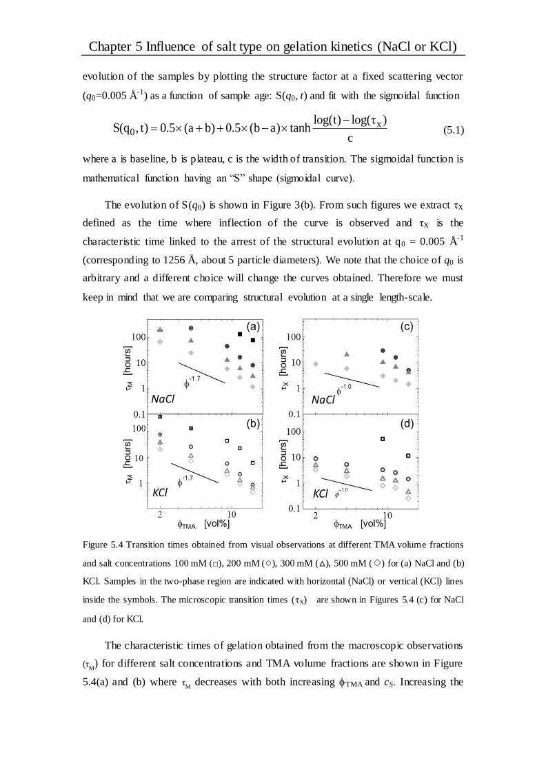
Chapter 5 Influence of salt type on gelation kinetics (NaCl or KCl)
evolution of the samples by plotting the structure factor at a fixed scattering vector
(q0=0.005 Å-1) as a function of sample age: S(q0, t) and fit with the sigmoidal function
x0
log(t) log( )S(q , t) 0.5 (a b) 0.5 (b a) tanh
c
(5.1)
where a is baseline, b is plateau, c is the width of transition. The sigmoidal function is
mathematical function having an “S” shape (sigmoidal curve).
The evolution of S(q0) is shown in Figure 3(b). From such figures we extract τX
defined as the time where inflection of the curve is observed and τX is the
characteristic time linked to the arrest of the structural evolution at q0 = 0.005 Å-1
(corresponding to 1256 Å, about 5 particle diameters). We note that the choice of q0 is
arbitrary and a different choice will change the curves obtained. Therefore we must
keep in mind that we are comparing structural evolution at a single length-scale.
Figure 5.4 Transition times obtained from visual observations at different TMA volume fractions
and salt concentrations 100 mM (□), 200 mM (○), 300 mM (△), 500 mM (◇) for (a) NaCl and (b)
KCl. Samples in the two-phase region are indicated with horizontal (NaCl) or vertical (KCl) lines
inside the symbols. The microscopic transition times (τX) are shown in Figures 5.4 (c) for NaCl
and (d) for KCl.
The characteristic times of gelation obtained from the macroscopic observations
(τM) for different salt concentrations and TMA volume fractions are shown in Figure
5.4(a) and (b) where τM
decreases with both increasing TMA and cS. Increasing the
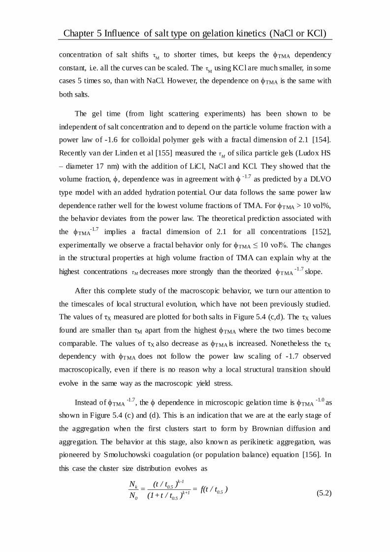
Chapter 5 Influence of salt type on gelation kinetics (NaCl or KCl)
concentration of salt shifts τM to shorter times, but keeps the TMA dependency
constant, i.e. all the curves can be scaled. The τM using KCl are much smaller, in some
cases 5 times so, than with NaCl. However, the dependence on TMA is the same with
both salts.
The gel time (from light scattering experiments) has been shown to be
independent of salt concentration and to depend on the particle volume fraction with a
power law of -1.6 for colloidal polymer gels with a fractal dimension of 2.1 [154].
Recently van der Linden et al [155] measured the τM
of silica particle gels (Ludox HS
– diameter 17 nm) with the addition of LiCl, NaCl and KCl. They showed that the
volume fraction, , dependence was in agreement with -1.7 as predicted by a DLVO
type model with an added hydration potential. Our data follows the same power law
dependence rather well for the lowest volume fractions of TMA. For TMA > 10 vol%,
the behavior deviates from the power law. The theoretical prediction associated with
the TMA-1.7 implies a fractal dimension of 2.1 for all concentrations [152],
experimentally we observe a fractal behavior only for TMA ≤ 10 vol%. The changes
in the structural properties at high volume fraction of TMA can explain why at the
highest concentrations τM decreases more strongly than the theorized TMA -1.7 slope.
After this complete study of the macroscopic behavior, we turn our attention to
the timescales of local structural evolution, which have not been previously studied.
The values of τX measured are plotted for both salts in Figure 5.4 (c,d). The τX values
found are smaller than τM apart from the highest TMA where the two times become
comparable. The values of τX also decrease as TMA is increased. Nonetheless the τX
dependency with TMA does not follow the power law scaling of -1.7 observed
macroscopically, even if there is no reason why a local structural transition should
evolve in the same way as the macroscopic yield stress.
Instead of TMA -1.7, the dependence in microscopic gelation time is TMA -1.0 as
shown in Figure 5.4 (c) and (d). This is an indication that we are at the early stage of
the aggregation when the first clusters start to form by Brownian diffusion and
aggregation. The behavior at this stage, also known as perikinetic aggregation, was
pioneered by Smoluchowski coagulation (or population balance) equation [156]. In
this case the cluster size distribution evolves as
k-1
k 0.50.5k+1
0 0.5
N (t / t )= = f(t / t )
N (1+t / t ) (5.2)

Chapter 5 Influence of salt type on gelation kinetics (NaCl or KCl)
where Nk is the number of clusters of size k and N0 the initial number of
monomers. This population density evolves in time following a single time-scale, the
half-life, that following Smoluchowski takes the form
0.5
S B 0
1 3η 1t = =
K w 4K Tρ w (5.3)
where kS is the Smoluchowski rate of aggregation as defined by diffusion. The term
W is the Fuchs stability ratio that takes into account the form of the inter-particle
potential which in turn depends on salt concentration. For the same salt concentration,
𝑡0.5 will scale as the inverse of the packing fraction as is observed in the data in
Figures 5.4 (c, d).
Interestingly, if we estimate the time at which the S(q0) stops evolving (time to
reach the plateau values in Figure 5.3 b) and compare it with τM we can see that for
most of the samples the gel becomes stress-bearing much before the structure has
been fixed at the scale of a few colloidal particles. This may suggest that particle
rearrangements take place at the microscopic scale, even if the gel is macroscopically
arrested. This might imply that the mechanical properties are still evolving, as we
shall see in the section 5.2.4.
5.2.4 Scaling
Now that we have seen the TMA dependence on both timescales, those data are
compared to better understand the effect of the salt concentration and type on the gel
formed. It has previously been shown that for a fixed particle volume fraction the
evolution of the structure and the mechanical properties of gels formed with different
concentrations of NaCl can be completely scaled onto a master curve by introducing
an appropriate gel time for normalization [154, 157, 158]. It was shown that changing
the concentration of NaCl only changes the kinetics of gelation and alters neither the
structure nor the strength of the gel formed thereafter.
Similarly, we now show that it is possible to scale both τM and τX. One can see in
Figures 5.4 that the TMA dependence is the same for all of the salt concentrations and
both salts. This means that we can use simple multiplicative constants to collapse all
the data, these constants are defined as βM and βX (the data with 500 mM of added
KCl have been chosen as a reference). Our rescaled data is shown in Figure 5.5,

Chapter 5 Influence of salt type on gelation kinetics (NaCl or KCl)
where we see a complete collapse of the data for both salts. Therefore we show that a
single constant works for a range of particle volume fractions. The values of β are
summarized in Table 1. One can note that in most cases, the values obtained for βM
and βX are the same, so in the following we will refer to the scaling factors β used
either for microscopic or macroscopic scaling.
Figure 5.5 The normalized transition times from the macroscopic observations MM (a) and from
the SAXS experiments XX (b).
Table 1 The scale factors β used to collapse the values of τM
and τX onto master curves for the
different salt concentrations and types.
The scaling of τX (extracted from S(q0,t)) indicates that at a given length-scale
the structural evolution is equivalent if the normalized time βt is used. Figure 5.6

Chapter 5 Influence of salt type on gelation kinetics (NaCl or KCl)
shows the full S(q) for 9 vol% TMA and 500 mM KCl and NaCl at βt = 3 hours. We
find that the curves coincide very well over the range of q values once again using the
scaling factor β. In the inset we show that the choice of β is appropriate over the full
evolution of the structure, as normalizing the time with β leads to a collapse of the
two S(q0). This means that variation of the structural evolution with the two salt types
can be fully captured by a single scaling factor.
Figure 5.6 Structure factor S(q) for the samples of 9vol% TMA and 500 mM salt with KCl at 3
hours (dashed line) and NaCl at 10 hours (solid line). The inset is shows S(q=0.005 Å) where the
time is scaled with βx for the same sample NaCl (empty symbols) KCl (filled symbols).
The M are linked to the mechanical properties of the gels, and we have seen that,
similarly with the structural variation, the time to reach a given yield stress can be
normalized by a scaling factor. This has led us to measure the storage and loss moduli
of a gel after 1, 4 and 100 days at fixed frequency 10 Hz and strain 1 % with TMA = 9
vol% cS = 500 mM for both salts. The kinetic dependencies of the moduli during the
gel- formation in the presence of both NaCl (filled symbols) and KCl (open symbols)
are presented in the inset in Figure 5.7. One can see that for both samples G’ and G’’
continue to increase with gel aging even after the macroscopic transition time is
elapsed. In addition it is clear that at a given time the values of G’ and G’’ are much
higher for gels formed with KCl compared to those with NaCl, at early times the
elastic modulus of a gel with KCl is more than 10 times higher than with NaCl. This
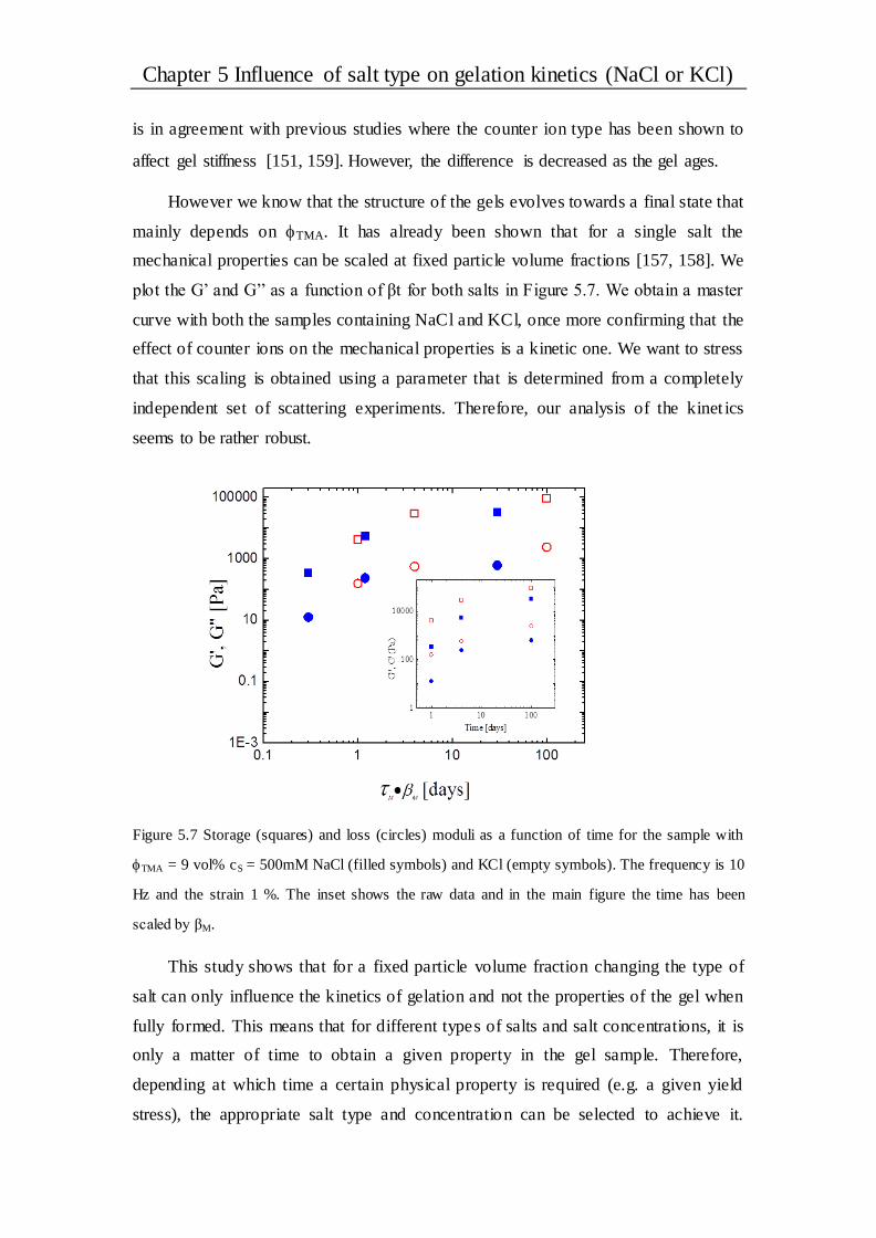
Chapter 5 Influence of salt type on gelation kinetics (NaCl or KCl)
is in agreement with previous studies where the counter ion type has been shown to
affect gel stiffness [151, 159]. However, the difference is decreased as the gel ages.
However we know that the structure of the gels evolves towards a final state that
mainly depends on TMA. It has already been shown that for a single salt the
mechanical properties can be scaled at fixed particle volume fractions [157, 158]. We
plot the G’ and G’’ as a function of βt for both salts in Figure 5.7. We obtain a master
curve with both the samples containing NaCl and KCl, once more confirming that the
effect of counter ions on the mechanical properties is a kinetic one. We want to stress
that this scaling is obtained using a parameter that is determined from a completely
independent set of scattering experiments. Therefore, our analysis of the kinet ics
seems to be rather robust.
Figure 5.7 Storage (squares) and loss (circles) moduli as a function of time for the sample with
TMA = 9 vol% cS = 500mM NaCl (filled symbols) and KCl (empty symbols). The frequency is 10
Hz and the strain 1 %. The inset shows the raw data and in the main figure the time has been
scaled by βM.
This study shows that for a fixed particle volume fraction changing the type of
salt can only influence the kinetics of gelation and not the properties of the gel when
fully formed. This means that for different types of salts and salt concentrations, it is
only a matter of time to obtain a given property in the gel sample. Therefore,
depending at which time a certain physical property is required (e.g. a given yield
stress), the appropriate salt type and concentration can be selected to achieve it.
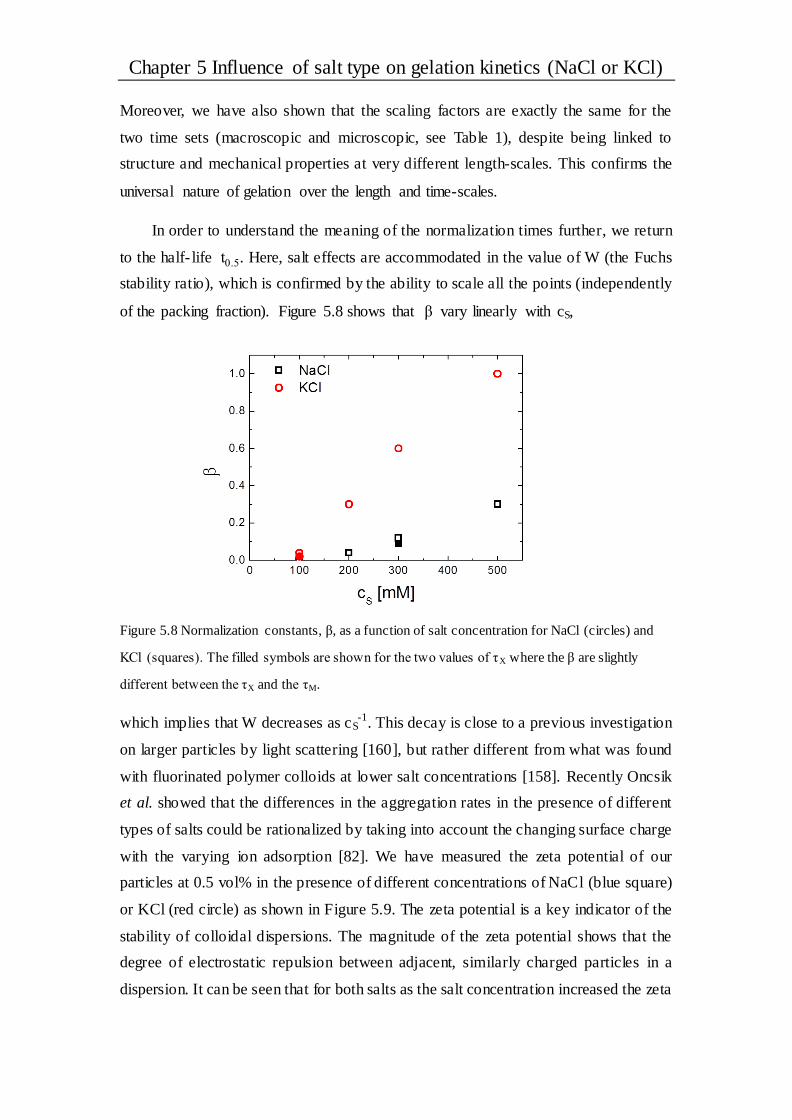
Chapter 5 Influence of salt type on gelation kinetics (NaCl or KCl)
Moreover, we have also shown that the scaling factors are exactly the same for the
two time sets (macroscopic and microscopic, see Table 1), despite being linked to
structure and mechanical properties at very different length-scales. This confirms the
universal nature of gelation over the length and time-scales.
In order to understand the meaning of the normalization times further, we return
to the half- life t0.5. Here, salt effects are accommodated in the value of W (the Fuchs
stability ratio), which is confirmed by the ability to scale all the points (independently
of the packing fraction). Figure 5.8 shows that β vary linearly with cS,
Figure 5.8 Normalization constants, β, as a function of salt concentration for NaCl (circles) and
KCl (squares). The filled symbols are shown for the two values of τX where the β are slightly
different between the τX and the τM.
which implies that W decreases as cS-1. This decay is close to a previous investigation
on larger particles by light scattering [160], but rather different from what was found
with fluorinated polymer colloids at lower salt concentrations [158]. Recently Oncsik
et al. showed that the differences in the aggregation rates in the presence of different
types of salts could be rationalized by taking into account the changing surface charge
with the varying ion adsorption [82]. We have measured the zeta potential of our
particles at 0.5 vol% in the presence of different concentrations of NaCl (blue square)
or KCl (red circle) as shown in Figure 5.9. The zeta potential is a key indicator of the
stability of colloidal dispersions. The magnitude of the zeta potential shows that the
degree of electrostatic repulsion between adjacent, similarly charged particles in a
dispersion. It can be seen that for both salts as the salt concentration increased the zeta

Chapter 5 Influence of salt type on gelation kinetics (NaCl or KCl)
potential increased too, and the zeta potential with KCl is always higher than with
NaCl. This suggests that more KCl is adsorbed on the particle surfaces, and it seems
that the differences in W could be the direct result.
A complete description of the microscopic mechanisms leading to the changing
kinetics of gelation is still missing, but adding our results to the other recent
observations of the strongly changing particle-particle interactions with ion type [92,
161, 162] should provide further testing ground for the predictions of the current
theories [41].
Figure 5.9 Zeta potential evolution with salt concentration in the presence of 0.5 vol%TMA, the
red circles are with KCl and blue squares with NaCl.
5.2.5 Gel rheology at a given time
From Figure 5.7, we know that at a given time the values of G’ and G’’ are much
higher for gel samples formed with KCl compared to those with NaCl. However, they
can be scaled onto a master curve by using the scaling factor β, which means that the
structures produced from both salts are the same after the gels have been allowed to
age significantly. It should be noticed that the strain used during the measurement in
Figure 5.7 is very small (1 % fixed) in order not to destroy the structure of the gels.
Nevertheless, it is worth to see what the structure response of gels formed with both
salts when the strain is gradually increased to destroy their structure.

Chapter 5 Influence of salt type on gelation kinetics (NaCl or KCl)
Storage modulus (G’) and loss modulus (G’’) of the gels were measured with the
sample TMA = 9 vol% in the presence of cS = 300 mM NaCl (blue circle) or KCl (red
square) 1 week after preparation as shown in Figure 5.10, where the strain rate is keep
constant at 5 s-1 and the strain is from 0.05 to 25. For both salts, the solid symbol is
corresponding to G’ and the open one is corresponding to G’’.
It can be seen that for both samples G’ and G’’ are constant when the strain is
small, this is because in the range of small strain the structure of the gels have not
been destroyed. Then as the strain continues to increase, G’ gradually decreases and
G’’ gradually increases after a certain point, where the structure of the gels start to be
destroyed. From Figure 5.10, one can note that there is a point at which the values of
G’ is equal to G’’. When the strain is exceeds than that point, the value of G’ is lower
than G’’, indicating the sample became from solid to liquid state. With NaCl the value
of strain at that point is 12.5 and with KCl is 10. The result shows that for NaCl it
needs higher strain to break the gel structure from solid to liquid state. It also can be
seen that the strain needed is higher with NaCl than KCl when G’ is began to decrease.
Therefore the gels formed with KCl are stronger at a certain point in time, although
they at long times they end up the same.
Figure 5.10 Storage modulus(solids) and Loss modulus(opens) evolved as strain with the sample
TMA = 9 vol% cS = 300 mM at strain rate 5 for KCl (red square) and NaCl (blue circle) after 1
week preparation. The strain of G’=G’’ with KCl is 10 and NaCl is 12.5.

Chapter 5 Influence of salt type on gelation kinetics (NaCl or KCl)
5.3 Conclusions
In this Chapter the salt-specific effects on the gelation process were investigated
through adding NaCl or KCl to a suspension of colloidal silica. Macroscopic
observations showed that the solidification with KCl is much faster than with NaCl.
This was in agreement with results obtained from SAXS experiments where the
evolution of the microstructure of the samples was followed and the characteristic
timescale of local structural arrest extracted. Both the macroscopic observations and
the local structure can be scaled onto a single master curve suggesting that the counter
ion type changes the timescale of gelation but not the equilibrium structure. This
equivalence of the structures over several length-scales is further confirmed by the
collapse of the storage and loss moduli when normalized with a scaling factor.
Further, the simple possibility to scale all our results suggests that the final gel
characteristics depend only on the volume fraction of TMA particles, at least when
salts such as NaCl or KCl are used. Mastering the properties of a gel is a very
important due to the range of applications in which they are found. This work
highlights that comparing properties of gels at times shortly after their formation can
be misleading if their long term characteristics are sought after.
The effect of salt in Soft Matter is extremely subtle. The Hofmeister series for
the precipitation and the “salting in” and “salting out” effects have been known for
more than a hundred years but their physical origin still remains elusive. In this work,
we have explored the effect of this observation on gelation. Indeed the two salts
explored here, result in different gelation times but the final gels are very similar in
structure and mechanical properties. This observation suggests that one could speedup
gelation without changing the structural properties of the final gel by simply choosing
the correct salt in the Hofmeister series.

Chapter 6 Influence of different salts on the gelation kinetics
Chapter 6 Influence of different salts on the
gelation kinetics
6.1 Introduction
In Chapter 5, the salts used for investigating ion specific effects on the gelation
process were NaCl and KCl. The results show that the counter ion type only changes
the timescales of gelation but not the equilibrium structure. It would be interesting to
see if the equivalence between the two salts can be extended to other monovalent salts
and even to divalent ones.
In this section, in addition to NaCl and KCl, the monovalent salts LiCl, CsCl and
a divalent salt MgCl2 are selected to study the ion effect on the gelation process by
adding salt to the suspension of silica particles. In Chapter 5, the betas we obtained
are from scaling of the macroscopic and microscopic timescales. We are wondering
that if there is an easier way to get the information of betas.
As an example, Figure 6.1 is the results of light transmission with samples 9vol%
TMA and 500 mM NaCl (open square) and KCl (open triangle). (a) is the normalized
transmitted light intensity with time using the formula( ) ( )
(0) ( )
I t I
I I
, where I(t) is the

Chapter 6 Influence of different salts on the gelation kinetics
transmitted light intensity in time, I(∞) is the transmitted light intensity after it stops
evolving and I(0) is the transmitted intensity at time t=0. It can be seen that the
normalized intensity decreases with time for both salts. However, the decrease is
faster with KCl than with NaCl. The transmission decreases as the particle size
increases. In our case it means that I is linked to the aggregation of TMA. This means
that the aggregation rate of silica particles in the presence of KCl is faster than with
NaCl. We already knew this from the SAXS experiments shown in the previous
chapter. All of the different measurements performed in Chapter 5 could be scaled
onto master curves using appropriate normalization constants. It would then seem
reasonable that the transmitted intensity could be too.
If indeed it can, it would be a simple way to get the information of relative
timescales of gelation with different kinds of salts.
Figure 6.1 Normalized transmitted light intensity evolved in time (a) and scaled time (b) with 9
vol% TMA and 500 mM NaCl (open square) and KCl (open triangle).
The good news is that the normalized transmission light intensity can be scaled
as shown in (b) and the two curves coincide very well. The scaling factor, called βI is
0.4, which compared with 0.3 obtained in Chapter 5 can be considered very good
within the experimental error.
Therefore, in this Chapter, we will use the light transmission method to
investigate the ion specific effects on the gelation process by adding salts MgCl2, LiCl,
NaCl, KCl, CsCl in the suspension of silica particles separately.
Chapter 6 Influence of different salts on the gelation kinetics
6.2 Results and discussion
6.2.1 General observation of gel samples
Four different kinds of monovalent and one bivalent salt are used in the light
transmission experiments. The range of TMA concentration is from 4 vol% to 16 vol%
and salt is from 100 mM to 500 mM. In this part, we take the middle concentration 9
vol% TMA and 300 mM salt as an example. The photographs of the samples at 0, 3
and 6 hours are shown in Figure 6.2. One can see that just after the samples prepared
at 0 hour, the color of the sample with CsCl is most dark, the rest of other salts are
lighter. With time increased to 3 hours, all of the samples became darker. Up to 6
hours, we can’t see much difference by eyes of the color changes except salt LiCl.
Figure 6.2 Photographs of samples with 9 vol%TMA and 300mM salt at 0, 3 and 6 hours. From
left to right, the salts are in order of LiCl, NaCl, KCl, CsCl and MgCl2.
The software Image J is used to extract the information of transmitted light
intensity with time. Figure 6.3 gives the normalized transmitted light intensity
evolution in time. As the gelation proceeds, the transmission decreased for all salts.
This is because of the aggregation of silica particles. The more aggregation proceeds

Chapter 6 Influence of different salts on the gelation kinetics
the less light is transmitted through the sample. The rate of aggregation is the fastest
with CsCl and slows down according to the order of salt CsCl > KCl > LiCl > MgCl2 >
NaCl.
Figure 6.3 Normalized transmitted light intensity as time in the presence of 9 vol%TMA and 300
mM LiCl (square), NaCl (circle), KCl (triangle), CsCl (diamond) and MgCl2 (star).
6.2.2 The scaling behavior
From Figure 6.1, we know that the curves of normalized transmitted light
intensity with time can be scaled onto the same curve in the presence of salt NaCl and
KCl. Now we are trying to know if the curves with all the salts used can be scaled,
Figure 6.4 shows the curves with all the salts after scaling in the presence of 9 vol%
TMA and 300 mM salt, βI is the time scaling factor. In order to keep the same way to
get βI, here the curve with 9 vol% TMA and 500 mM KCl was fixed as reference,
whose value was considered as 1, then we shift the curves with other kinds of salt
onto it. The scaling factors βI are given in Table 1 following the salt order: LiCl
(0.042) < NaCl (0.15) < MgCl2 (0.24) < KCl (0.67) <CsCl (2.1). Together with the
normalized transmitted light intensity in Figure 6.3, we know that the aggregation rate
was faster with larger value of βI. One can see that all the curves coincide extremely
well. It suggests that the evolution with different kinds of salts can be scaled at fixed
silica and salt concentration.
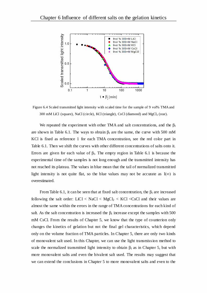
Chapter 6 Influence of different salts on the gelation kinetics
Figure 6.4 Scaled transmitted light intensity with scaled time for the sample of 9 vol% TMA and
300 mM LiCl (square), NaCl (circle), KCl (triangle), CsCl (diamond) and MgCl2 (star).
We repeated the experiment with other TMA and salt concentrations, and the βI
are shown in Table 6.1. The ways to obtain βI are the same, the curve with 500 mM
KCl is fixed as reference 1 for each TMA concentration, see the red color part in
Table 6.1. Then we shift the curves with other different concentrations of salts onto it.
Errors are given for each value of βI. The empty region in Table 6.1 is because the
experimental time of the samples is not long enough and the transmitted intensity has
not reached its plateau. The values in blue mean that the tail of normalized transmit ted
light intensity is not quite flat, so the blue values may not be accurate as I(∞) is
overestimated.
From Table 6.1, it can be seen that at fixed salt concentration, the βI are increased
following the salt order: LiCl < NaCl < MgCl2 < KCl <CsCl and their values are
almost the same within the errors in the range of TMA concentrations for each kind of
salt. As the salt concentration is increased the βI increase except the samples with 500
mM CsCl. From the results of Chapter 5, we know that the type of counterion only
changes the kinetics of gelation but not the final gel characteristics, which depend
only on the volume fraction of TMA particles. In Chapter 5, there are only two kinds
of monovalent salt used. In this Chapter, we can use the light transmiss ion method to
scale the normalized transmitted light intensity to obtain βI as in Chapter 5, but with
more monovalent salts and even the bivalent salt used. The results may suggest that
we can extend the conclusions in Chapter 5 to more monovalent salts and even to the

Chapter 6 Influence of different salts on the gelation kinetics
bivalent salt. These may as well indicate that the scaling behavior of specific ion
effect on the aggregation of colloidal particles is universal.
Table 6.1 Scaling factors βI are obtained by taking 500 mM KCl (red color) as reference for each
volume fraction of silica particles. The range of TMA is from 4 vol% to 16 vol% and salt
concentration is from 100 mM to 500 mM. The values in blue indicate that the experimental time
is not long enough to get the flat tail in the transmission, so the value maybe not accurate. In the
empty region the gelation time of the samples is longer than the experimental time.
The scaling factor βI reflects the aggregation rates of silica particles, which
means that the aggregation rates increased following the above salt order and as the
salt concentration increased except for the sample with 500 mM CsCl. When
observing the values of βI with CsCl, one can see that there is a peak at 300mM as the
concentration of CsCl increased. This implies that at 300 mM the aggregation rate of
silica particles is fastest. Then if we continue to increase the concentration of CsCl the
aggregation rate decreased. It seems that this behavior is contradictory to other salts.

Chapter 6 Influence of different salts on the gelation kinetics
However, many studies have shown that a strong adsorption of the counter ion onto
the particle surface, which can lead to its charge reversal [82, 92]. Moreover, the
recent research shows that the ion specific effects in the aggregation process are
mainly because of the variation in ion adsorption changing the surface charge [82]. In
our case, the aggregation of silica particles is the fastest in the presence of CsCl,
which suggests that the interaction of Cs+ is the strongest with the surface. At some
point, when the adsorption is enough the surface charge will reverse and the
aggregation rate will decrease as at 500 mM CsCl. The good thing is that even the
surface charge is reversal the gelation process still can be scaled.
6.2.3 Half-time of the transmitted intensity
Another way to look at the transmitted data is to compare the time it takes for the
intensity to decrease by half, and this time is defined as τhalf. This time could be linked
to the aggregation similarlty to τX, but at a larger length-scales. Figure 6.5 gives the
relationship between τhalf and the volume fraction of TMA with all the monovalent
salts used. (a) is with LiCl, (b) with NaCl, (c) with KCl and (d) with CsCl, the range
of salt concentration used is from 100 mM to 500 mM and TMA is from 4 vol% to 16
vol%.
All the data decreased as the volume fraction of silica particles increased and the
salt concentration increased. From (a) to (d), the τhalf with LiCl is the largest and CsCl
is the smallest at a fixed salt and silica concentration. The volume fraction
dependence of power law -1.7 is plotted in each graph in Figure 6.5. Rather
surprisingly, we can be seen that the τhalf of first three kinds of salt follow the -1.7
dependence very well. It means that the transmission probes length-scales are
sufficiently large, which linked to the gel structure but not to the initial small
aggregation like τX in Chapter 5.
However, for the salt of CsCl as given in Figure 6.5(d), the overall trend of the
data follows the same linear relationship, but there have deviation at some points. The
data are very close for different concentrations of CsCl except 100 mM at the range of
TMA volume fraction. This is because that the aggregation of silica particles with
CsCl is very fast. The transmitted light intensity decreased by half is accomplished in
less than 10 minutes for most of the samples. Before taken the photos, it will spend 2

Chapter 6 Influence of different salts on the gelation kinetics
or 3 minutes for sample preparation. For the sample with slower gelation time, the
sample preparation time can be neglected compared with τhalf. However, for the
sample with CsCl, its value is comparable with τhalf. Therefore, for this kind of salt the
time τhalf we got may not be accurate.
Figure 6.5 The time of normalized transmission light intensity decreased by half with monovalent
salt (a) LiCl, (b) NaCl, (c) KCl and (d) CsCl. The range of salt concentration is from 100 mM to
500 mM and υTMA is from 4 vol% to 16 vol%.
Figure 6.6 The time of normalized transmission light intensity decreased by half with divalent salt
MgCl2. The range of salt concentration is from 100 to 500 mM and TMA is from 4 vol% to 16
vol%.

Chapter 6 Influence of different salts on the gelation kinetics
The time of normalized transmission light intensity decreased by half with
divalent salt MgCl2 is shown in Figure 6.6. The line -1.7 is also plotted in the graph
and all data are agreed well with the -1.7 dependence although the salt is bivalent.
Moreover, the relationship between the data and υTMA and the salt concentration have
the same trend as the monovalent salt. The results suggest that the ions with different
valence have the same mechanism on the effects of gelation process.
From Figure 6.5 and 6.6 we can see that the volume fraction variation leads to a
power law -1.7 for the τhalf for both monovalent and bivalent salts at all concentrations
used (only the CsCl shows some deviation). Because τhalf is just one point of the full
intensity curves we have collapsed in 6.2.2, they should be scalable onto a master
curve as well using the βI we already obtained in Table 6.1. The scaled data is given in
Figure 6.7, where we can see the good collapse for all salts even there are some
scattered points, which are attributed to the salt with CsCl. The advantage to look at
τhalf is to see dependence, which we can’t obtain from the intensity I(t).
Figure 6.7 The normalized time of transmitted light intensity decreased by half for the different
salt concentrations and types with the volume fraction of silica particles.
6.2.4 Stability of the gel system
Figure 6.8 shows the relationship of 1/βI and normalized salt concentration.
Mg2+is the bivalent ion, so we need to normalize it by multiplying by 2 when
comparing the results with monovalent salt. As discussed above, the scaling factorsβI

Chapter 6 Influence of different salts on the gelation kinetics
are almost the same at all volume fractions of TMA particles for a given salt
concentration. Therefore, the data in Figure 6.8 with 4, 9, 12, 16 vol% TMA are
almost the same. With the first three kinds of salt, all data decrease as the salt
concentration increased. However, with KCl and CsCl, the data seem to stop
decreasing at the higher concentrations and even increase a little with CsCl.
Figure 6.8 The inverse of scaling factor, 1/βI, as a function of normalized salt concentration for
MgCl2 (square), LiCl (diamond), NaCl (circle), KCl (up triangular), and CsCl (down triangular) in
the presence of 4 vol% TMA (a), 9 vol% TMA (b), 12 vol % TMA(c) and 16 vol % TMA(c).
From Chapter 5, we showed that 1/βI is proportional to the Fuchs stability ratio
W, which is linked to the interparticle potential. The interactions are different and the
height of the potential barrier is the lowest with CsCl, probably because the charge of
the TMA is lower. As discussed in 6.2.2 that the specific ion effects on the
aggregation process is due to the ion adsorption onto the surface charge. At higher salt
concentrations, excess absorbed the counterions can lead to the surface charge
reversal [92]. This can explain why the W with CsCl at higher salt concentration is a
little bit increased. We could imagine that with further increase in the salt
concentration, the other salts may have the same trend.
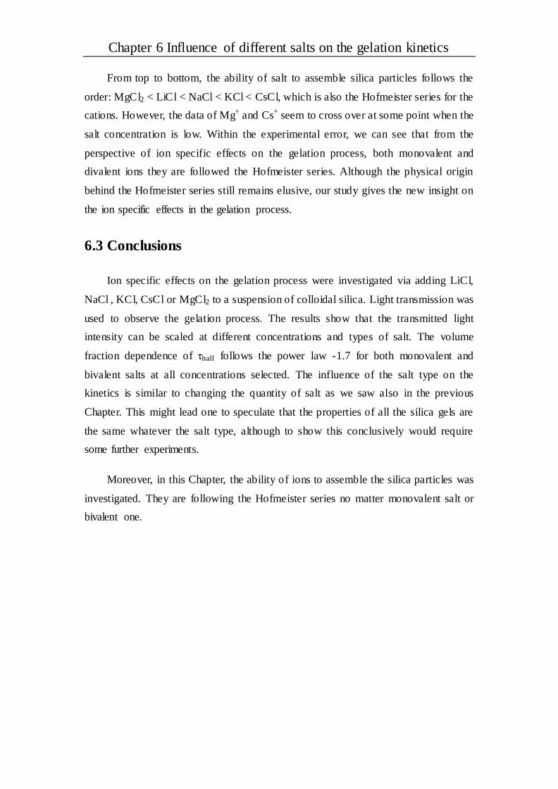
Chapter 6 Influence of different salts on the gelation kinetics
From top to bottom, the ability of salt to assemble silica particles follows the
order: MgCl2 < LiCl < NaCl < KCl < CsCl, which is also the Hofmeister series for the
cations. However, the data of Mg+ and Cs+ seem to cross over at some point when the
salt concentration is low. Within the experimental error, we can see that from the
perspective of ion specific effects on the gelation process, both monovalent and
divalent ions they are followed the Hofmeister series. Although the physical origin
behind the Hofmeister series still remains elusive, our study gives the new insight on
the ion specific effects in the gelation process.
6.3 Conclusions
Ion specific effects on the gelation process were investigated via adding LiCl,
NaCl , KCl, CsCl or MgCl2 to a suspension of colloidal silica. Light transmission was
used to observe the gelation process. The results show that the transmitted light
intensity can be scaled at different concentrations and types of salt. The volume
fraction dependence of τhalf follows the power law -1.7 for both monovalent and
bivalent salts at all concentrations selected. The influence of the salt type on the
kinetics is similar to changing the quantity of salt as we saw also in the previous
Chapter. This might lead one to speculate that the properties of all the silica gels are
the same whatever the salt type, although to show this conclusively would require
some further experiments.
Moreover, in this Chapter, the ability of ions to assemble the silica particles was
investigated. They are following the Hofmeister series no matter monovalent salt or
bivalent one.

Chapter 6 Influence of different salts on the gelation kinetics

Chapter 7 Mixed salt and surfactant to make ultrastable and
stimulable foam
Chapter 7 Mix salt and surfactant to make
ultrastable and stimulable foam
7.1 Introduction
Foams are found in a wide variety of applications in industry and personal life,
such as firefighting, enhanced oil recovery, mineral flotation, food processing and
personal care products. In some of these applications good foam stability is extremely
important. All foams are thermodynamically unstable and are destined to disappear
[163]. In order to prolong their life, various types of stabilizing agents are used, such
as surfactants, polymers, proteins or particles [56]. These stabilizing agents adsorb
onto the surfaces of the bubbles and slow down the different mechanisms by whic h
foams age: drainage, coalescence and coarsening.
In some cases foams that are stable for very long periods of time are required, so
called ultrastable foams, in which the processes of coarsening and drainage should be
arrested. Previous studies have shown that the ultrastable liquid foam can be made
using the dispersions of lamella liquid crystals [164], hydrophilic particles [65],
mixed surfactant [165] and so on. Ultrastable foams have many applications in

Chapter 7 Mixed salt and surfactant to make ultrastable and
stimulable foam
industry such as shown above in firefighting, enhanced oil recovery, mineral flotation.
However, in other cases, good foam stability is initially required but at a given
moment it should become unstable and disappear. Therefore, the destruction of foam
is often required in practical applications. The foams should be stimulable. The foam
stability can be tuned by the external stimuli parameters such as pH, magnetic fields,
temperature and so on [166-171].
In this Chapter, we add NaCl or KCl to SDS to make ultrastable and temperature
stimulable foam. We show that foam stability is controlled by the formation of
crystals on the surface of the bubbles and in the aqueous phase. The time it takes for
the crystals to form is the key factor to obtain stable foams. These ultrastable foams
can be destroyed by heating above the Krafft boundary (below which precipitates
form).
The work in this Chapter has finished and the results have been published: Zhang,
Li, et al. "Precipitating Sodium Dodecyl Sulfate to Create Ultrastable and Stimulable
Foams." Angewandte Chemie 127.33 (2015): 9669-9672.
7.2 Results and discussion
7.2.1 Foamability and foam stability with fixed SDS at room
temperature
Foams were prepared using 69 mM SDS with added NaCl or KCl. Photographs
of these foams as they evolve in time are shown in Figure 7.1. Samples in (a) and (b)
were made with 250 mM and 500 mM of NaCl, while samples in Figures 7.1 (c), (d)
and (e) were with KCl. The solutions with NaCl foam very well, all of the gas is
incorporated in the foam. The foam with 250 mM NaCl disappears within 2 ho urs
(even more quickly than foam with no added salt) as shown in 7.1 (a). With 500 mM
NaCl given in Figure 7.1 (b), most of the foam collapses quickly but the remaining
foam continues to evolve slowly: the bubble size increases while the height of the
foam remains constant over several hours.
The instability of the foam with 250 mM added NaCl could be expected. The
screening of the electrostatic repulsion between the two interfaces dominates over the
effect of the increased surface concentration of surfac tant and the films become

Chapter 7 Mixed salt and surfactant to make ultrastable and
stimulable foam
unstable. The stability of the foam with 500 mM NaCl after an initial phase of foam
collapse is surprising.
The behavior with KCl is very different as seen in Figures 7.1 (c) and (d). The
foams produced are very similar with the two KCl concentrations. Not all of the air
can be incorporated into the foam and even when the amount of liquid used is
increased. We can only make around 8 mL of foam with an initial liquid fraction of
around 50 %. We have not been able to make dry foams, only bubbly liquids. In a
matter of seconds the bubbles have creamed to the top of the sample, and as they
become close packed (liquid fraction around 30 – 40 %) the drainage slows down
dramatically, but continues over several hours before arresting. The coarsening in
these samples arrests as well. This leads to ultrastable foams, and as shown in Figure
7.1 (e), the foam is still intact after 6 months.
Figure 7.1 Photographs of foam samples made with 69 mM SDS and (a) 250 mM NaCl; (b) 500
mM NaCl; (c) 250 mM KCl; (d) 500 mM KCl, (e) sample (d) 6 months later.
We have also prepared foams from KDS with added KCl (69 mM with 500mM
salt). These are much less convenient to work than their SDS homologues as the
KDS solution needs to be heated up above the Krafft boundary (around 50 °C) to
prepare the foams. However their appearance and stability are very similar to those
from SDS with added KCl. In this Chapter we will mainly talk about the foam
prepared with SDS.

Chapter 7 Mixed salt and surfactant to make ultrastable and
stimulable foam
In order to understand these differences we take a closer look at the samples. We
can see some precipitate at the bottom of the flask in Figure 7.1 (b), but nothing with
KCl in Figure 7.1 (d). We made optical microscopy experiments on bulk samples
(without foaming). In both samples the precipitates are composed of crystals. The
crystalline domains formed with NaCl as given in Figure 7.2(a) are plate-like
structures of tens of micrometers in size while the objects with KCl are smaller as
shown in Figure 7.2(b).
Figure 7.2 Microscope images of solution with 69 mM SDS and 500 mM NaCl (a) and KCl (b)
taken a day after mixing. Images of bubbles immediately after preparation prepared with the same
concentrations, NaCl (c) and KCl (b).
Table 7.1 Temperature at which the crystals are no longer visible in the presence of 69 mM SDS
with 250 or 500 mM salt.
The samples were heated to measure the temperature at which the crystals are no
longer visible by eye (Table 7.1). From these values the enthalpies of dissolution, H,

Chapter 7 Mixed salt and surfactant to make ultrastable and
stimulable foam
can be estimated using the Van’t Hoff equation. We find HSDS = 75 kJmol-1 and
HKDS = 88 kJmol-1. Like previously reported by Smith et al. [172], the enthalpy for
the melting of SDS is slightly lower than KDS. However assuming that the energy
gain of sodium is 84 kJmol-1 more than for potassium [144], the interaction energies
are weaker in KDS than in SDS.
Figures 7.2(c) and (d) show photographs of bubbles taken under the microscope
immediately after the generation of foaming the samples. The foam with NaCl (Figure
7.2c) looks exactly like normal surfactant foam: it is rather wet and the bubbles have a
diameter of around 200 µm. The sample with KCl looks nothing like a surfactant
foam (Figure 7.2d): the bubbles are much smaller (mostly below 100 µm in diameter)
and the larger bubbles are not spherical but ellipsoidal.
The presence of elliptical bubbles is surprising as the optimal shape for an air
bubble is spherical. A non-spherical shape indicates that the interfaces are solid-like
[173]. Therefore coarsening of bubbles is arrested making the foam stable (addition of
KCl).
From Figure 7.2 (a) and (b) we know that the precipitates of solution with 69
mM SDS and 500 mM NaCl or KCl without foam are composed of crystals. In the
foam with 500 mM NaCl, the solution collected at the bottom of the vial is slightly
turbid. This implies that not all crystals are inside the foam. The solution that drains
out of the foams prepared with KCl is transparent, despite a non-foamed solution
being turbid. This means that the crystals can get trapped and collect in the Plateau
borders, to stabilize the foam against drainage [174, 175]. In Figure 7.2(d), the
solid-like bubble surfaces in the presence of KCl show this.
The stability of the foams with KCl can therefore be explained by the formation
of the crystals on the bubble interfaces and in the interstices between the bubbles.
However the relative instability of the foam with NaCl is still not entirely clear.
7.2.2 Influence of changing SDS concentration on foam generation
and stability
Photographs of foam prepared with 100 mM KCl at various SDS concentrations
(35, 69, 139 and 277 mM) are shown in Figure 7.3. The foam immediately after
preparation is shown in (a), one hour after preparation in (b) and 7 hours later in (c).

Chapter 7 Mixed salt and surfactant to make ultrastable and
stimulable foam
The graph (7.3.d) shows the evolution of the foam height for these samples in time.
The height of generated foam, which we will term foamability increased with
increased SDS concentration. Not all of the gas incorporated into the foam samples
except the sample with 277 mM SDS.
For the samples with 35, 69 and 139 mM SDS, the produced foams are loosely
packed as one can see in (a), there are many big bubbles in the foam. However, after
one hour, it seems that most of the bubbles have disappeared (7.3.d the foam height
changed little after one hour) and the foams can be stable at least for several months.
Furthermore, in Figure d, it looks that there is an optimum concentration of SDS to
make the maximum of stable foam near 139 mM.
Figure 7.3 Photographs of foam samples made with 100 mM KCl and 35, 69, 139, 277 mM SDS.
(a) Foam after prepared. (b) Foam after prepared 1 hour. (c) Foam after prepared 7 hours. (d)
Measurement of foam height with SDS concentrations at different hours.
Then for the sample with 277 mM SDS, the foamability is the best (the largest
volume of foam is produced) and the produced foam is the most homogeneous with a
small bubble size. However, the foam is unstable. As one can see, after one hour, due
to the drainage and coarsening, the foam has changed a lot. In fact, it’s much more
like a dry network structure than a foam. There are no discernable bubbles left and the
structure is connected by the white crystals and it’s very brittle. The network like
structure is unstable and collapses to the bottom with time as shown by the foam
height change in (d).

Chapter 7 Mixed salt and surfactant to make ultrastable and
stimulable foam
Photographs of foam prepared with 250 mM KCl at various SDS concentrations
(35, 69, 139 and 277 mM) are shown in Figure 7.4. The foam immediately after
preparation is shown in (a), 3 hours after preparation in (b) and 7 hours later in (c).
The graph (7.3.d) shows the evolution of the foam height for these samples in time.
One can see that the foamability increased with increased SDS concentration. For
most of the samples not all of the gas could be incorporated into the foam.
For the foams produced with 35, 69,139 and 277 mM SDS, they quickly drain
after preparation, after which the drainage slows down dramatically before completely
arresting. The coarsening of the foam samples arrest as well. However, for the foam
with 412 mM SDS, if you observe it carefully, you can see that the foam is unlike the
foams to the left of it. This foam is like the foam produced with 277 mM SDS and
100 mM KCl. Their aging process are very similar, but the difference is that the foam
with 250 mM KCl needs longer time to become a dry looking network like structure
with crystalline collection in the Plateau borders, which also needs longer time to
collapse.
Figure 7.4 Photographs of foam samples made with 250 mM KCl and 35, 69, 139, 277, 412 mM
SDS. (a) Foam after prepared. (b) Foam after prepared 3 hours. (c) Foam after prepared 7 hours.
(d) Measurement of foam height with SDS concentrations at different hours.
Indeed, at 7 hours it can be seen that the network like structure has already
started to form. For the other foams, they can stable at least for several months. The
foam height after arresting has linear relationship with the SDS concentration. It is
increased with the increased SDS concentration as seen in (d). Moreover, from (d) one

Chapter 7 Mixed salt and surfactant to make ultrastable and
stimulable foam
can note that the foam behavior changes at the concentration of 139 mM SDS.
Compared with 35 and 69 mM SDS, the foamability raises suddenly and the foam
height falls strongly after one hour, which means that at higher SDS concentration the
foambility is increased. Although the foam will collapse to a certain point after
preparation the foam is still stable.
A third concentration of KCl was explored at 500 mM. Photographs of foam
prepared with 500 mM KCl at various SDS concentrations (35, 69, 139 and 277 mM)
are shown in Figure 7.5. The foam immediately after preparation is shown in (a), 3
hours after preparation in (b) and 7 hours later in (c). The graph (7.3.d) shows the
evolution of the foam height for these samples in time. One can see that the
foamability increased with increased SDS concentration. Not all of the gas
incorporated into the foam samples.
Figure 7.5 Photographs of foam samples made with 500mM KCl and 35, 69, 139, 277, 412 mM
SDS. (a) Foam after prepared. (b) Foam after prepared 3 hour. (c) Foam after prepared 7 hours. (d)
Measurement of foam height with SDS concentrations at different hours.
The initial liquid fractions of these foams from left to right are around 20 %,
51 %, 43 %, 39 % and 34 %. One can note that the liquid fraction is decreased with
the increased SDS concentration except for the sample with 35 mM SDS. This is
correct because more foam can be made at higher SDS concentration but the total
liquid volume is fixed. Then in a matter a seconds the bubbles have creamed to the
top of the samples, as the foam become close packed (liquid fraction from left to right
around 13 %, 45 %, 40 %, 33 % and 31 %) the drainage and coarsening slow down

Chapter 7 Mixed salt and surfactant to make ultrastable and
stimulable foam
dramatically, but continues over several hours before arrests. One hour later, the
foams height is almost unchanged except the one with 412 mM SDS as seen in (d),
which needs longer time to age. After the foams arrest, the foam height is increased
with the increased SDS concentration. The relationship between them is approximate
linear. When the salt concentration is higher than SDS, maybe the amount of
produced crystals is proportional to the SDS concentration. That is why the foam
crystals can stablise it proportionally as well. All the foam samples obtained with 500
mM KCl and the given SDS concentrations are ultrastable, they can be stable more
than 6 months at room temperature.
Figures 7.3, 7.4 and 7.5 show that for the foam samples at fixed salt
concentration foamability is increased as the surfactant concentration increased and
most of the foams are ultrastable. However, for the sample with 277 mM SDS in
Figure 7.3 and with 412 mM SDS in Figure 7.4, the formed foams are unstable and
the foam ageing is not like the normal foam. The foam ages to the network-like
structure first and then collapse to unstable the foam. When compared with the
ultrastable foams, one can see that for this kind of foam samples the surfactant
concentration used is much higher that the salt concentration used.
The foamability is much better at fixed salt concentration with higher surfactant
concentration, which means that much more foam can be produced. However, the
total quantity of crystal is constant so that for each bubble there might not be enough
crystals to stabilize it. We’ll get back to the reasons behind what’s going on after
having looked at the kinetics of crystal formation.
7.2.3 Kinetics of crystals formation
In order to explain the instability of the NaCl foams, we have measured the time
after which the crystals become visible to the eye when the samples are cooled down
from a homogeneous state. In order to keep the same condition for the samples, each
time we heated the samples 1℃higher that the dissolution temperature measured in
7.2.1 to get a homogeneous solution. Then we cooled to the target temperature and
recorded the time at which crystals appeared. The times are shown in Figure 7.6 (a).
The crystallization time (tc) is increased as T is decreased. T is the temperature
difference between the dissolution temperature and the target temperature. In all the

Chapter 7 Mixed salt and surfactant to make ultrastable and
stimulable foam
T range, tc with NaCl is higher than with KCl. It takes at least twice as long for
each T. This means that the crystallization kinetics is considerably slower with
NaCl than with KCl.
Figure 7.6 (b), (c), (d) and (e) are the foam samples prepared with 69 mM SDS
and 500 mM salt at different T and different times. (b) and (c) are with KCl, when
T=20 ℃, tc is smaller than 1min and the foam aging is rapidly arrested and the
bubbles remain very small. Ultrastable foam can be obtained in this condition. When
T=8 ℃, tc increases to around 3 minutes, the foam ageing is eventually arrested as
the crystals form, however the resulting material is more like a crystal network-like
structure than an aqueous foam and it is very brittle, like the foam formed with 277
mM SDS in Figure 7.3 and 412 mM SDS in Figure 7.4, will collapse finally. (d) and
(e) are with NaCl, at T=8 ℃ and 5 ℃, tc increases to around 5 min and 10 min
respectively. Under this condition, the foam has enough time to evolve and it will
partially collapse before the ageing can arrest, like in (d) and (e). tc with T=8 ℃ is
smaller compared with T=5 ℃, so there is more foam left with T=8 ℃.
Figure 7.6(a) Time for the precipitate to become visible by the naked eye after cooling. (b)
Photographs of foam at different times with T=8 ℃ and tc ≈ 3 min. (c) Photographs of foam at
different times with T=20 ℃ and tc ﹤1 min. (d) Photographs of foam at different times with
T=5 ℃ and tc ≈ 3 min. (e) Photographs of foam at different times with T=8 ℃ and tc ≈ 5 min.
Figures b and c are with 500 mM KCl and d and e with 500 mM NaCl. 69 mM SDS was used for
all the samples.
The investigated kinetics of crystal formation given in Figure 7.6 can explain the
instability of the NaCl foams. For the samples shown in Figure 7.1, it takes tens of

Chapter 7 Mixed salt and surfactant to make ultrastable and
stimulable foam
minutes for the crystals to appear in the sample with NaCl, but with KCl they appear
within seconds of mixing. Therefore in the sample with NaCl the foam has ample
time to evolve (coarsen, coalesce and drain) before the crystals form and can start
stabilizing the foams. Similarly making foams with low concentrations of added KCl
(with SDS or KDS) leads to relatively unstable foams, as the crystallization process is
slower than the destabilization process.
However, there is another situation that can exist as shown in Figure 7.6 (b), the
formed foam with KCl is unstable (a crystal network- like structure and collapse)
although the crystallization time is not very long. When compare the samples (b) and
(c), one can note that the difference between them is foamability (b is higher than c).
This indicates that unstable foam will obtain if much more foam produced but there
are not enough crystals to stabilize it even the crystal formation kinetics is not so slow.
From foam formed with 277 mM SDS in Figure 7.3 and 412 mM SDS in Figure 7.4,
we can get the same conclusion. However, for this part, the detailed mechanisms
about how the network-like structure formed need more experiments.
This means that whether the foam is stabilized depends on the link between the
kinetics of crystal formation and the foam ageing times, as well as how much foam is
produced at certain formed crystals. If crystallization is too slow the foam has time to
evolve and it will partially collapse or totally disappear before the ageing can arrest.
Or if too much foam is produced the formed crystals are not enough to stabilize it.
The stability of the foams from both SDS and KDS with added KCl suggest that it is
not the presence of a mixture of counter ions that is determinant in the stabilization
process (Na+ and K+). The requirement seems to be for the presence of potassium and
dodecyl sulfate in sufficient concentration and at a temperature below the Krafft
boundary. Of course the Krafft boundary should depend strongly on the solution and it
is sensitive to the type and concentration of ions present, i.e. DS- and Cl-, with Na+
and/or K+.
7.2.4 Structure of crystallites inside the foam
We have carried out SANS measurements on the foams prepared with 69 mM
SDS and 500 mM NaCl or KCl. The foam made with NaCl partially collapsed during
the experiment. The medium and high q data from the foam with NaCl were

Chapter 7 Mixed salt and surfactant to make ultrastable and
stimulable foam
multiplied by a factor 4 in the data treatment, to compensate for the disappearance of
scattering material during the measurement. The scattered intensity as a function of q
for the two samples is shown in Figure 7.7 (a) where we can see that at low q the
intensity decreases as q-4. Such decay is typical of sharp interfaces, such as the
surfaces of the bubbles and the crystallites.
We can also distinguish two peaks arising from the crystal structure in Figure
7.7(b). For the sample with NaCl, the first peak is at q* = 0.16 Å-1 and the second one
at 0.32 Å-1, so twice the first one. The sample with KCl has peaks at 0.19 Å-1 and 0.38
Å-1. The structure of SDS crystals has been previously measured, they have been
shown to have a lamellar structure where the inter-planar distance, d, depends on the
degree of chain tilt and hydration [176]. We measure d = 39 Å (2π/q*) for the SDS
crystals (precipitated with NaCl). This is exactly what has been measured when SDS
is crystallized from water, it forms monoclinic weakly hydrated (SDS · 1/8 H2O)
crystals with d = 38.9 Å [176]. The crystals formed with KCl also have a lamellar
structure, however the spacing is smaller than with SDS at d = 33 Å. Due to the large
difference in the crystallization temperatures, the crystals should be almost
exclusively of KDS. This means that the KDS crystals are more tightly spaced than
SDS, suggesting that the KDS crystalline unit cell is more strongly tilted.
Figure 7.7 (a) The scattered intensity as a function of the wave vector for a foam prepared with 69
mM SDS and 500 mM NaCl (red circles) and 500 mM KCl (blue squares). In (b) the high q data is
shown in a linear scale.

Chapter 7 Mixed salt and surfactant to make ultrastable and
stimulable foam
7.2.5 Stimulating the foam by temperature
The photograph of Figure 7.1(e) shows that foam prepared with 69 mM SDS and
50 mM KCl can be stable for at least 6 months at room temperature. We have shown
that the incredible stability of the foam arises from the presence of crystallized KDS
both at the surfaces of the bubbles and in the interstices between the bubbles. In order
to break it we heat it to 51°C to melt the crystals. The images are shown in Figure 7.8.
The bubbles shown in Figure 7.8(a) have rugged surfaces and some precipitates are
also found in the surrounding fluid. Very quickly the surface of the bubbles starts to
melt, as seen in the photograph taken after 13 s. The bubbles start coarsening and
coalescing, before disappearing in a few minutes.
Figure 7.8 Bubbles (a) and foams (b) prepared with 69 mM SDS and 500 mM KCl heated
suddenly to 51°C.
We can see the same effect on bulk foam in Figure 7.8(b). Within one minute the
drained solution has become transparent. The foam starts to age as the crystals
disappear from the foam, although this probably takes some time as foam is a very
poor heat conductor. After 1 minute some liquid has drained, and after around 10
minutes the bubble size starts to change considerably. The melting of the crystals
(bulk and interfacial) transforms the foam into common wet foam, which disappears

Chapter 7 Mixed salt and surfactant to make ultrastable and
stimulable foam
within a few hours.
The produced foams are temperature stimulable. It is also possible to stop the
foam ageing before all the foam has disappeared to reform a s table foam again. We
have prepared a sample of foam with 69 mM SDS and 500 mM KCl as shown in
Figure 7.9, which is ultrastable at room temperature as already known in the previous
part. The foam has been left to age for an hour at room temperature after preparation,
then suddenly put in the water bath with the temperature of 51 °C, which is higher
than the dissolution temperature of crystals formed at the surfaces of the bubbles and
in the interstices between the bubbles.
The drained solution in 51 s in the photograph has become transparent. The foam
starts to age as the crystals melt from the foam as shown in the photograph at 88 s,
some of the foam has disappeared. The foam is left to destabilise for 2 minutes after
which it is plunged into a water bath at room temperature. The crystals start to reform
and the ageing of the foam is slowed down (at 143 s). As the crystals reform we find
many of them in the drained solution at the bottom of the foam sample (the solution is
turbid). These crystals will eventually reform and sediment to the bottom of the
sample (at 70 min). The ageing of the reformed foam sample will arrest after several
hours, and it is still very stable at room temperature (we have given 4 days, but it can
remain stable longer than 4 days).
Figure 7.9 Foam prepared with 69 mM SDS and 500 mM KCl at room temperature and waited for
1 hour. Then the foam was placed in a water bath at 51°C and taken out after 120 s and placed in
another water bath at room temperature (T = 22 °C). The foam sample also was given after 4 days
at room temperature.
We show that the process can be stopped and started, however the resulting foam
is different as the concentration of crystals changes due to the drainage of the

Chapter 7 Mixed salt and surfactant to make ultrastable and
stimulable foam
surfactant solution.
7.3 Conclusions
The addition of salt at a high concentration can be used to make ultrastable
foams from SDS. Stable foams are made below the Krafft temperature. However
whether the foams are stable or not also depends on the kinetics of crystal formation.
This can be tuned via the preparation temperature by changing the type and
concentration of added salt. If crystallization is too slow, the foam has time to
disappear. If the crystals have time to form on the surfaces of the bubbles the foams
are stable over months or until they are heated to melt the crystals at which point they
start to age and disappear quickly. Nevertheless, there is one exception, unstable foam
still can be obtained if too much foam produced at certain formed crystals even the
crystal formation kinetics is not so slow, like the concentration of surfactant is much
higher than salt in our case. This can be controlled by selecting appropriate sample’s
concentration.
We have shown how the crystallization of surfactant can be used to our
advantage in creating ultrastable or/and stimulable foams. We have also seen that the
addition of KCl is much more efficient than NaCl. However the detailed mechanisms
including the importance of the presence of two types of counter ions in the foams
with KCl, or the role of the crystal structure on foam stability still require further
experiments and/or simulations.
These results are important as they provide a simple way of making very stable
foams. They could be used in applications where the self- life of a product should be
measured in months or years without degradation of the quality of the foam. Thanks
to their sensitivity to temperature they could even be used as simple temperature
sensors to indicate prolonged heating during a transport phase. However their main
quality is their simplicity, superstability and stimulability become affordable for more
applications.

Chapter 8 Foam aging modified by the gel phase
Chapter 8 Foam aging modified by the gel
phase
8.1 Introduction
Solid foams are found in a wide variety of materials, and this makes
understanding the process of making solid foam so important. It is one of the simple
methods to prepare very light porous ceramic materials, which have various
applications in areas such as tissue engineering , thermal or acoustic insulation,
heterogeneous catalysis, and chromatography due to their low mass density and high
surface area [177-181]. So it’s important to know how to control their properties such
as mechanical, thermal or acoustic and so on. To do this we need to understand the
evolution of the microstructure of the foam.
Solid foam is made from the precursor of wet foam, in which the continuous
phase needs to be either solidified or gelified. Solid silica foams are produced by
drying the silica–loaded wet foams for production of porous materials [182, 183]. If
the continuous phase is becomes a gel, as the gelation process proceeds, the viscosity
of the gel phase will first increase and it will acquire a certain elasticity. From Chapter
5 and 6, we know that a gel can be formed by adding salt to the suspension of silica

Chapter 8 Foam aging modified by the gel phase
particles. Therefore, in this Chapter, salt was added to the suspension of silica
particles to produce the gel phase, which was used as the continuous phase of the
foam to slow down and even arrest the foam ageing. We use a mixture of N2 with
traces of C6F14 (perfluorohexane) to slow down the coarsening and SDS is used as
surfactant to generate the foam.
8.2 Results and discussion
8.2.1 The evolution of bubbles in the gel foam
A range of samples was investigated with different TMA and salt concentrations:
9 vol% TMA and 500 mM NaCl; 12 vol% TMA and 300 mM NaCl; 12 vol% TMA
and 500 mM NaCl; 16 vol% TMA and 300 mM NaCl; 16 vol% TMA and 200 mM
NaCl. All the samples also had 10 g/L SDS, which means that when considering the
ionic strength of the solutions we should also take into account the 69 mM of Na+.
The reason to select these concentrations is because the macroscopic gelation times
measured range in a few hours, which is a typical aging time of foams (they will
coarsen and drain, but will not disappear within this time, hence giving us the
possibility to arrest the foam ageing before they are gone). In addition, the sample 300
mM NaCl 10 g/L SDS without particles used as reference. The photographs of foam
at 1 and 3 hours are given in Figure 8.1 for each concentration with the bulk liquid
volume fraction υl and the averaged bubble radius R.
All the foams are prepared with the same initial liquid fractionΦl of 14.3 %.
After generation the foam ages. Looking at the liquid fractions we can see that they
drain to around 7 % within one hour after which the drainage slows down and the
liquid fraction changes little in the next 2 hours. The bubbles also coarsen, and the
average bubble size increases for all the samples. In all the samples the Φl and the
average radius are different. If you look at the photographs carefully, you can find that
the shapes of the bubbles have differences as well. Some of them are not spherical
anymore, and not because of the foam becoming very dry. For example, the bubbles
for sample in (c) and (e) at 3 hours.
Before running this experiment, we measured the macroscopic gelation times for
the samples without SDS (this was done exactly like in Chapter 5 to get the τM). From

Chapter 8 Foam aging modified by the gel phase
(a) to (e) the gelation times are 65 min, 131 min, 30 min, 271 min and 55 min. The
gelation time of the samples in (c) and (e) are faster than other samples. Therefore, we
could expect that the ageing of the foam in these two samples is the most influenced
by the bulk gel phase.
Figure 8.1 Photographs of bubbles at 1 hour and 3.0 hours in the presence of 9 vol%TMA 500 mM
NaCl (a), 12 vol%TMA 300 mM NaCl (b), 12 vol%TMA 500 mM NaCl (c), 16 vol%TMA 200
mM NaCl (d), 16 vol%TMA 300 mM NaCl (e), and 300 mM NaCl (f). For all the concentrations,
SDS was used at 10 g/L.
We will now look at the distribution of bubble radii in the first 6 hours, and these
are shown in Figure 8.2. The samples are the same as those in Figure 8.1. In the first 2
hours, one can see that the peaks of the curves decrease and shift to a higher radius as
the foam ages for all the samples. Then for the next several hours, in (a), (b), (d) and
(f), the peaks of the curves continue to decrease but very slowly as they shift to the
higher radii as well. For these samples the foam aging is slowed down. However, for

Chapter 8 Foam aging modified by the gel phase
comparison in (c) and (e), the peaks of the curves are unchanged after 3 hours, which
indicates that the foam aging of these two samples is arrested.
Figure 8.2 The distribution of numbers of bubbles as a function of radius in the first 6 hours. (a)
with 9 vol%TMA 500 mM NaCl, (b) with 12 vol%TMA 300 mM NaCl, (c) with 12 vol%TMA
500 mM NaCl, (d) with 16 vol%TMA 300 mM NaCl, (e) with 16 vol%TMA 200 mM NaCl, and
(f) with 300 mM NaCl. For all the concentrations, SDS used was 10 g/L. 0 hour (square), 1 hour
(circle), 2 hours (UpTriangular), 3 hours (down triangular), 4 hours (diamond), 5 hours (star), and
6 hours (pentagon).
In fact, from Figure 8.2, it can be seen that the change of bubble distribution is

Chapter 8 Foam aging modified by the gel phase
only fast in the first 1 hour, this is consisitant with the result of liquid fraction
obtained in Figure 8.1. After that the foam aging is slowed down or arrested
depending on the the different salt and TMA concentrations used.
As foam ages, the shapes of the bubbles are not spherical anymore. So in our
case, we only calculate the radius of the bubbles in the first 7 hours by using the
equation S=πr2 and consider that they are still spherical. The normalized radii as a
function of time are given in Figure 8.3(a). Here the radius taken is as the average
radius. Because the graph is in log- log scale, the data at t=0 is not shown. One can
note that in the first 7 hours, the radii of the bubbles evolves as a power law for the
samples with 9 vol% TMA 500 mM NaCl, 12 vol% TMA 300 mM NaCl, 16 vol%
TMA 200 mM NaCl and the reference sample 300 mM NaCl and they have the
similar slopes, which are slightly smaller than 0.5. However, the samples with
concentration of 12 vol% TMA 500 mM NaCl and 16 vol% TMA 300 mM NaCl
stopped to increase at t=4 hours. In the linear part, the slope of former is lower than
0.3 and the latter is higher than 0.3.
Figure 8.3 Normalized bubble radius (a) and normalized bubble numbers (b) with time for the
concentration 9 vol%TMA 500 mM NaCl (square), 12 vol%TMA 300 mM NaCl (circle), 12
vol%TMA 500 mM NaCl (up triangular), 16 vol%TMA 200 mM NaCl (diamond), 16 vol%TMA
300 mM NaCl (down triangular), and 300 mM NaCl (star). The linear lines t0.3
and t0.5
are shown
in (a).
When you look at the power law showing the relationship between the average
bubble radius and time, it is funny that the power law is not going as 0.5 as the
standard surfactant foams that coarsen and age normally. However, for our samples
the continuous phases of foams are gel phases, it is interesting to see that the power
Chapter 8 Foam aging modified by the gel phase
laws of them are close to 0.5 or 0.3. Moreover, it can be seen from the data that the
growth of the bubbles can be stopped for the samples same as in Figure 8.1 (c) and (e),
then for the rest of them their growth rate of the bubbles are similar like the reference
sample without gel phase. This is a proof to show that the ageing of the foam can be
influenced by the bulk gel phase.
The normalized number of bubbles as a function of time are given in Figure 8.3
(b). One can see that all the data decrease with time. The data dropped slowest for the
sample with concentration 12 vol%TMA 500 mM NaCl and fastest one is 16
vol%TMA 200 mM NaCl, other samples are between them. Moreover, it can be seen
from Figure 8.3 (b) that the time taken for the number of bubbles to reduce to half of
its original value is much slower for sample 12 vol%TMA 500 mM NaCl (about 4
hours) than sample 16 vol%TMA 200 mM NaCl (about 1 hour).
8.2.2 The mechanical properties of the bulk gel phase
In order to understand why the ageing of the foam is influenced as it is, we did
measurements of the bulk rheological properties. The measurement process was as
follows: the samples are transferred into the Double Gap immediately after
preparation and we wait for 1 hour for the gel to form, and then start the measurement
Figure 8.4 Storage modulus (G’) and Loss modulus (G’’) as a function of time with 9 vol%TMA
500 mM NaCl (square), 12 vol%TMA 300 mM NaCl (circle), 12 vol%TMA 500 mM NaCl (up
triangular), 16 vol%TMA 200 mM NaCl (pentagon), and 16 vol%TMA 300 mM NaCl (diamond).
The solid symbols corresponding to G’ and open symbols G’’.

Chapter 8 Foam aging modified by the gel phase
with 1 % strain and 1 Hz frequency for 2.5 hours, so at the end of the measurement
the sample age is 3.5 hours. Storage modulus (G’) and loss modulus (G’’) evolution
with time are shown in Figure 8.4. For all the concentrations, like the mechanical
properties measured in Chapter 5, G’ are higher than G’’ and both moduli increase
with time. G’ and G’’ also varied with the concentration used.
8.2.3 The effect of gel strength on foam aging
It is known that an elastic modulus of the fluid forming the foam can strongly
change the ageing process of the foam. The drainage and coarsening can be slowed
down and even arrested. We could imagine that if the coarsening process is slowed
down a lot by the elastic modulus of the gel, the radius of the bubbles should depend
on the G’ of the gel at a given time. Therefore, we have plotted R as a function of G’.
The relationship of R and G’ for all the concentrations in the first 3 hours is obtained
from the previous part as shown in Figure 8.5, (a) is the normalized radius and (b) is
the average bubble radius. There are many factors that influence the growth of the
bubble size, for example the silica and the salt concentrations. As seen in Figure
8.5(b), it is complicated to say something about the relationship between R and G’.
Therefore, in the following we discuss the relationship between the normalized R and
G’ in Figure 8.5(a), as this seems more reasonable.
The three points for each symbol from left to right show the values of R and G’
(of the bulk phase not the foam) at 1 hour, 2 hours and 3 hours respectively. Keeping
in mind the data in Figure 8.3(a), we know that the growth of the bubbles continued in
the first 7 hours for the samples with lower concentrations of TMA and NaCl and
stopped after 4 hours for the two concentrations with high TMA and/or NaCl (12:500
and 16:300). Therefore, we can see that the silica gels can be sufficiently strong to
arrest the growth of the bubbles leading to stable foam. Simulations of the conditions
of arrest have been carried out by Fyrillas [184] et al. However, their results are
difficult to compare with our experimental values.

Chapter 8 Foam aging modified by the gel phase
Figure 8.5(a) Normalized radius with storage modulus G’ for the concentration 9 vol%TMA
500 mM NaCl (square), 12 vol%TMA 300 mM NaCl (circle), 16 vol%TMA 200 mM NaCl
(diamond), 12 vol%TMA 500 mM NaCl (down triangular), and 16 vol%TMA 300 mM NaCl
(hexagon). (b) is the average radius corresponding to the normalized one. The three points from
left to right for each symbol represent 1 hour, 2 hours and 3 hours. The growth of the bubbles will
arrest after 4 hours for the samples with green triangles and purple hexagons.
From Figure 8.3 (a), we know that the bubble’s radius does not always continue
to grow. The samples with purple and green symbols will stop their growth at 4 hours.
Nevertheless, as shown in Figure 8.5(a), the slopes between R and G’ are not the same
for these two samples. In other words, the values of G’ are different for them to arrest
the foam aging. Therefore, we can conclude that there should be a critical point of the
gel strength to stable the foam. That is to say, if G’ is less than the critical point, the
radius of the bubbles continues to grow and the foam is unstable; if it is above the
critical value, they arrest. Because of the evaporation of the samples in the rheometer,
we only obtained the gel strength in the first 3 hours. In order to ascertain whether the
reasoning is correct we should do more detailed measurements of foam rheology.
As discussed above, it is known that the gel strength is an important factor to
influence the foam stability, with higher gel strength comes higher stability of the
foam. However, if we compare the data with purple and green symbols, blue and
black or red symbols in Figure 8.5(a), you can find that the former have larger G’ and
bubble size. It seemed that this is contradictory to the gel strength analysis above.
Nevertheless, if you see the two sets of data listed carefully, you can see the salt
concentrations are different. The former has lower salt concentration than the latter.
Chapter 8 Foam aging modified by the gel phase
We can say that the foam aging is influenced much more strongly by the salt
concentration than the particle volume fraction. This can be shown in Figure 8.3,
although the gel phase is exists in the sample 16 vol% TMA 200 mM NaCl, the
evolution of its bubble size and numbers are still faster than the reference sample,
which has the salt concentration of 300 mM. Moreover, we already know from
Chapter 5 that with higher salt the gelation process is faster.
Therefore, we can conclude that the gel strength and gelation kinetics are two
important factors to modify the foam aging.
8.2.4 Correlation behavior
In the previous section, we know that the gel strength and gelation kinetics are
important factors to slow down or arrest the foam aging. In this case, the movement of
the bubbles for the samples with higher gel strength and salt concentration should be
slower than others. The correlation behavior can compare the movement at certain
time to the previous time. Therefore we use the software Image J to obtain the
correlation map and the correlation coefficient R between two images. Correlation
map is a map showing the difference between the local areas. Correlation coefficient
reflects how much the two images related. Higher R means more closely related. The
time interval between two images is 5 minutes. First 20 images of the samples with
the concentration 16 vol% TMA 200 mM NaCl and 16 vol% TMA 300 mM NaCl are
selected to do the measurement (in 95 min). By doing this, the next image is
considered as the target and the previous one considered as the source. The correlation
sequence is from target to the source.
As an example, Figure 8.6 shows the correlation map with correlation coefficient
R (a) is 0.215 and (b) is 0.937. The color of the correlation map is darker with small R
and lighter with large R. R is small means the bubbles in the next image have strong
movement based on the previous image; otherwise, the movement of the bubbles is
not so obvious in the next image.
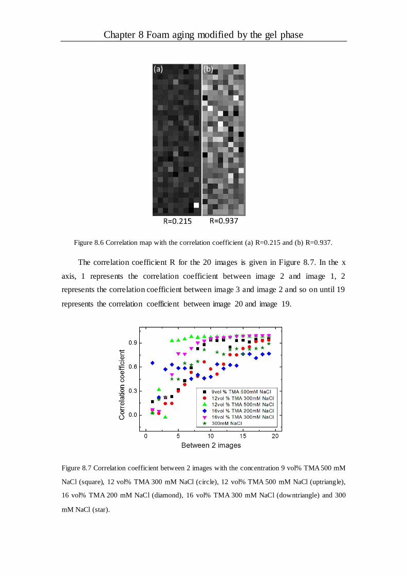
Chapter 8 Foam aging modified by the gel phase
Figure 8.6 Correlation map with the correlation coefficient (a) R=0.215 and (b) R=0.937.
The correlation coefficient R for the 20 images is given in Figure 8.7. In the x
axis, 1 represents the correlation coefficient between image 2 and image 1, 2
represents the correlation coefficient between image 3 and image 2 and so on until 19
represents the correlation coefficient between image 20 and image 19.
Figure 8.7 Correlation coefficient between 2 images with the concentration 9 vol% TMA 500 mM
NaCl (square), 12 vol% TMA 300 mM NaCl (circle), 12 vol% TMA 500 mM NaCl (uptriangle),
16 vol% TMA 200 mM NaCl (diamond), 16 vol% TMA 300 mM NaCl (downtriangle) and 300
mM NaCl (star).
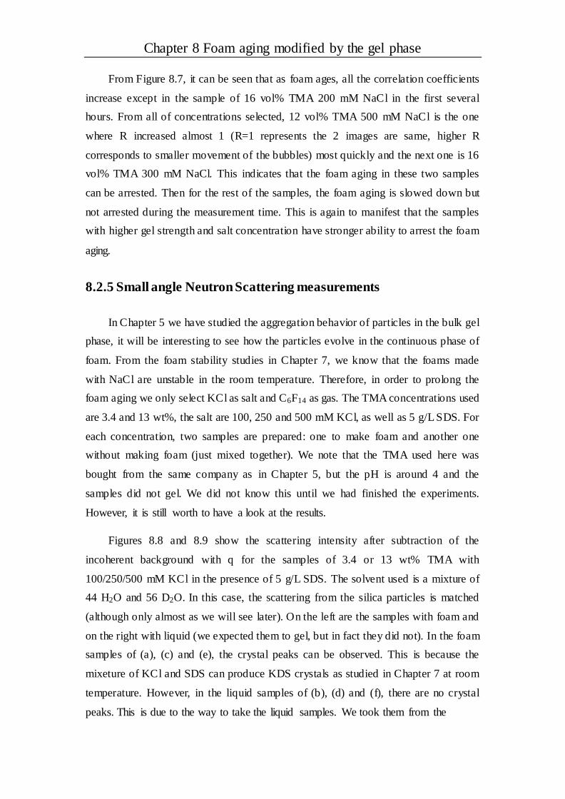
Chapter 8 Foam aging modified by the gel phase
From Figure 8.7, it can be seen that as foam ages, all the correlation coefficients
increase except in the sample of 16 vol% TMA 200 mM NaCl in the first several
hours. From all of concentrations selected, 12 vol% TMA 500 mM NaCl is the one
where R increased almost 1 (R=1 represents the 2 images are same, higher R
corresponds to smaller movement of the bubbles) most quickly and the next one is 16
vol% TMA 300 mM NaCl. This indicates that the foam aging in these two samples
can be arrested. Then for the rest of the samples, the foam aging is slowed down but
not arrested during the measurement time. This is again to manifest that the samples
with higher gel strength and salt concentration have stronger ability to arrest the foam
aging.
8.2.5 Small angle Neutron Scattering measurements
In Chapter 5 we have studied the aggregation behavior of particles in the bulk gel
phase, it will be interesting to see how the particles evolve in the continuous phase of
foam. From the foam stability studies in Chapter 7, we know that the foams made
with NaCl are unstable in the room temperature. Therefore, in order to prolong the
foam aging we only select KCl as salt and C6F14 as gas. The TMA concentrations used
are 3.4 and 13 wt%, the salt are 100, 250 and 500 mM KCl, as well as 5 g/L SDS. For
each concentration, two samples are prepared: one to make foam and another one
without making foam (just mixed together). We note that the TMA used here was
bought from the same company as in Chapter 5, but the pH is around 4 and the
samples did not gel. We did not know this until we had finished the experiments.
However, it is still worth to have a look at the results.
Figures 8.8 and 8.9 show the scattering intensity after subtraction of the
incoherent background with q for the samples of 3.4 or 13 wt% TMA with
100/250/500 mM KCl in the presence of 5 g/L SDS. The solvent used is a mixture of
44 H2O and 56 D2O. In this case, the scattering from the silica particles is matched
(although only almost as we will see later). On the left are the samples with foam and
on the right with liquid (we expected them to gel, but in fact they did not). In the foam
samples of (a), (c) and (e), the crystal peaks can be observed. This is because the
mixeture of KCl and SDS can produce KDS crystals as studied in Chapter 7 at room
temperature. However, in the liquid samples of (b), (d) and (f), there are no crystal
peaks. This is due to the way to take the liquid samples. We took them from the

Chapter 8 Foam aging modified by the gel phase
Figure 8.8 Scattering intensity I(q) after subtraction the incoherent background I_bcg as a function
of q for the samples with 3.4 wt% TMA at various salt concentrations in the presence of 5 g/L
SDS. The samples on the left side are foam and right side are liquid. (a) and (b) with 100 mM KCl,
(c) and (d) with 250 mM KCl, and (e) and (f) with 500 mM KCl. The solvent is the mixture of
H2O and D2O (44:56). The red line is the form factor of silica particles. Solid square symbol
represents the foam sample and open square one represents the liquid sample.
bottom and the crystals are on the top. It is difficult to say something from the figures,
but we can estimate the liquid fraction in the foam from the incoherent scattering.
This is linked to the flat background measured at high q. We take the intensity of foam
and divide it by the liquid one. In the figures the red line is a calculated form factor of

Chapter 8 Foam aging modified by the gel phase
silica particles. When we match silica, in the liquid samples with 13 wt% TMA, from
the shape of the curves it seems that we still can see the silica particles slightly. In
these samples the measured intensity is very low, we did not have enough statistics.
Figure 8.9 Scattering intensity I(q) after subtraction the incoherent background I_bcg as a function
of q for the samples with 13 wt% TMA at various salt concentrations in the presence of 5 g/L SDS.
The samples on the left side are foams and right side are liquids. (a) and (b) with 100 mM KCl, (c)
and (d) with 250 mM KCl, and (e) and (f) with 500 mM KCl. The solvent is the mixture of H2O
and D2O (44:56). The red line is the form factor of silica particles. Solid square symbol represents
the foam sample and open square one represents the liquid sample.

Chapter 8 Foam aging modified by the gel phase
The measured values of foam liquid fraction from the data in Figures 8.8 and 8.9
are shown in Table 1. One can see that with 3.4 wt% TMA Φl is increased with salt
concentration except for 250 mM KCl when the scattering form silica particles is
matched. Although the errors in these measurements are rather important due to the
insufficient measurement times for some of the samples, the tendency seems logical.
We know that the foams are more stable with the higher concentrations of salts.
However, with 13 wt% TMA the maximum Φl is with 250 mM KCl, which is a little
strange. But it is not easy to explain why it is like this.
Table 1 Volume fraction of the samples calculated from Figure 8 to 11.
Figures 8.10 and 8.11 are the same concentration as in Figures 8.8 and 8.9. The
difference is that the solvents used are a mixture of 92 H2O and 8 D2O. In this
condition, air is matched. In (a), (c) and (e) for all the foam samples, we can see the
crystal peaks as when we match the silica particles, but not in the liquid samples in (b),
(d) and (f). Moreover, we can see the nice shape of the scattering curves coincides
exactly with the form factor P(q) of silica particles. This means that the silica particles
can be seen inside the foams as well as the gels. However, it seems that the silica
particles have not started aggregating and the increase in the scattered intensity at low
q is mainly because of the gas/liquid interfaces.

Chapter 8 Foam aging modified by the gel phase
Figure 8.10 Scattering intensity I(q) after subtraction the incoherent background I_bcg as a
function of q for the samples with 3.4 wt% TMA at various salt concentrations in the presence of 5
g/L SDS. The samples on the left side are foams and right side are liquids. (a) and (b) with 100
mM KCl, (c) and (d) with 250 mM KCl, and (e) and (f) with 500 mM KCl. The solvent is the
mixture of H2O and D2O (92:8). The red line is the form factor of silica particles. Solid square
symbol represents the foam sample and open square one represents the liquid sample.

Chapter 8 Foam aging modified by the gel phase
Figure 8.11 Scattering intensity I(q) after subtraction the incoherent background I_bcg as a
function of q for the samples with 13 wt% TMA at various salt concentrations in the presence of 5
g/L SDS. The samples on the left side are foams and right side are liquids. (a) and (b) with 100
mM KCl, (c) and (d) with 250 mM KCl, and (e) and (f) with 500 mM KCl. The solvent is the
mixture of H2O and D2O (92:8). The red line is the form factor of silica particles. Solid square
symbol represents the foam sample and open square one represents the liquid sample.

Chapter 8 Foam aging modified by the gel phase
In order try to understand more about the behavior of silica particles in the foam
sample, we show an apparent structure factor S(q) with concentration 13 wt% TMA
250 mM KCl 5 g/L SDS when air is matched is given in Figure 8.12. We have divided
the scattered intensity by the calculated P(q) of the silica particles at the given
concentration. One can see that S(q) is increased with decreasing q, but we are not
sure the scattering is from the surface of silica particles or the crystals. Anyway, it’s
interesting to see the silica particles in foam sample. This part needs more
experiments.
Figure 8.12 Structure factor S(q) evolved as q for the foam sample with the concentration of 13 wt%
TMA 250 mM KCl and 5 g/L SDS when air is matched. The solvent is the mixture of H2O and
D2O (92:8).
8.3 Conclusions
In this Chapter the modification of the foam aging by the gel phase was
investigated by mixing NaCl or KCl, silica particles, SDS and C6F14 to produce gel
foam. A reference sample was selected without particles. The results of liquid fraction
show that the drainage of foam is fast in the first one hour and then it slowed in the
next hours. This is consistent with the distribution of bubble sizes, the changement of
which is only fast in the first hour. After that, the peaks of the distribution curves
slowly shift to the higher radius except the samples with 12 vol% TMA and 500 mM
NaCl and 16 vol% TMA and 300 mM NaCl, for these the curves are stopped to shift
after 3 hours. When look at the normalized radius with time, one can find that the
radii of them stopped to increase at around 4 hours. These suggest that foam aging is

Chapter 8 Foam aging modified by the gel phase
arrested with these two samples.
The rheological properties of bulk gel phases are measured, the relationship
between R and G’ imply that gel strength and gelation kinetics are two important
factors to slow down or arrest the foam aging. For the samples of 12 vol% TMA with
500 mM NaCl and 16 vol% TMA with 300 mM NaCl they have high gel strength and
smallest gelation time. That is the reason why they can arrest the foam aging. For rest
of them they only can slow down of it. The correlation behavior is another proof to
manifest that the gel strength and gelation kinetics are two important factors to
modify the foam aging.
These results are useful as they provide a simply way to make solid foam. Foam
aging can be tuned by changing the concentration of salt and particles in the sample.

Chapter 9 Conclusions
Chapter 9 Conclusions
The dissertation is focused on the pattern of phase separation in the miscibility
gap, ion specific effects on the aggregation of colloidal part icles and surfactant, and
gel phase influences to the foam stability.
We have observed the macroscopic and microscopic phase separation processes
at various conditions using a microscope and scanning electron microscopy (SEM).
The structure and the mechanical properties of gels are investigated by small angle
X-ray scattering (SAXS) and rheology methods. Small angle neutron scattering
(SANS) measurements are performed to determine the structure of crystallites inside
the foam. The detailed conclusions are summarized as below:
1. In the miscibility gap, SD and NG type phase separations have been
investigated. The results show that layer structures can be formed for both types under
the thermal gradient but their morphologies are not the same. This is due to their
distinct kinetic characteristics and the volume fraction of the minority phase. For SD
type, it has a higher growth rate and volume fraction of minority phase leading to fast
aggregation. As shown in the microscopic evolution of SD type, when the para meters
are controlled appropriately, multilayer structures can be obtained. This is feasible for
NG type as well. However, the difference is that for the former the minority phase

Chapter 9 Conclusions
rich layer is composed of the big aggregates of the minority phase and for the latter is
the distribution of minority phase as spherical droplets.
Further, the initial structure characteristics of these two types of phase separation
are not the same. According to this, different morphologies can be obtained such as
the Fe-Sn ribbon. Our studies show that NG and SD type phase separations both in the
early and late stage can produce different morphologies.
2. NaCl or KCl is added to a suspension of colloidal silica to investigate the
salt-specific effects on the gelation process. Macroscopic observations and
microscopic structure from SAXS experiments showed that the solidification with
KCl is much faster than with NaCl. It’s found that the macroscopic observations and
the local structure can be scaled onto a single master curve, indicating that the counter
ion type changes the timescale of gelation but not the equilibrium structure. The
collapse of the storage and loss moduli when normalized with a scaling factor is
further confirmation of the equivalence of the structure over several length-scales.
The results also indicate that one could speedup gelation without changing the
structural properties of the final gel by simply choosing the correct salt in the
Hofmeister series.
When salts such as NaCl or KCl used it’s possible to scale all results, suggesting
that the final gel characteristics depend only on the volume fraction of TMA particles.
The rheology measurements as a function of strain show that the strain needed to
destroy the gel structure is higher with NaCl than with KCl, implying that the gel
structure with NaCl is more flexible than with KCl even its storage modulus is less
strong, when they are compared at a given time. Of course at long times they seem to
tend to the same.
3. The light transmission method is used to observe the gelation process by
adding different kinds of salt to the dispersion of silica particles. The normalized
transmitted light intensities can be normalized by a scaling factor for all
concentrations and types of salt selected, as well as the time (τhalf) when the
transmitted light intensity decreased by half. This suggests that at least the scaling
behavior with NaCl or KCl in Chapter 5 can be extended to more monovalent salts
and even to divalent ones.
The ability of ions to assemble the silica particles has been investigated as well.

Chapter 9 Conclusions
It is found that they are following the Hofmeister series no matter monovalent salt or
bivalent one.
4. The addition of salt at a high concentration to SDS has been studies. It’s
shown that ultrastable foams are made below the Krafft temperature. However
whether the foams are stable or not also depends on the kinetics of crystal formation.
If crystallization is too slow, the foam has time to disappear. If the crystals have time
to form on the surfaces of the bubbles the foams are stable over months or until they
are heated to melt the crystals at which point they start to age and disappear quickly.
Nevertheless, there is one exception, unstable foam still can be obtained if too much
foam is produced at a certain quantity of formed crystals even the crystal formation
kinetics is not so slow. Such that the concentration of surfactant is much higher than
salt. This can be controlled by selecting appropriate sample concentrations. Moreover,
the type of salt with KCl is much more efficient than NaCl in creating ultrastable
or/and stimulable foams.
5. The foam aging modification by the gel phase is investigated by mixing salt,
silica particles and surfactant solution to produce gelling foam. The results of
averaged bubble size and rheology measurements suggest that the gel strength is the
important factor to restrict the growth of the bubbles, which are smaller when the gel
strengths are higher. Comparing the bubble size data of sample 16 vol% TMA and
300 mM NaCl with 12 vol% TMA and 500 mM NaCl or sample with 16 vol% TMA
and 200 mM NaCl with a reference sample, we found that gelation kinetics is another
factor to influence the evolution of bubbles. The aging of foam with lower salt
concentration is faster than with higher one.

Bibliography
Bibliography
[1] Walter H. U., Fluid sciences and materials science in space: a European perspective . 2012:
Springer Science & Business Media.
[2] Roozeboom B., HW: Heterogene Gleichgewichte, 1901, Braunschweig.
[3] Ratke L., Immiscible liquid metals and organics. 1993: DGM Informationsgesellschaft
Verlag.
[4] Cardy J., Phase transitions and critical phenomena. Vol. 11Academic, London, 1987.
[5] Bates F. S.Wiltzius P., Spinodal decomposition of a symmetric critical mixture of
deuterated and protonated polymer. The Journal of chemical physics, 1989. 91(5): p.
3258-3274.
[6] Cumming A., Wiltzius P., Bates F. S., Rosedale J. H., Light-scattering experiments on
phase-separation dynamics in binary fluid mixtures. Physical Review A, 1992. 45(2): p.
885.
[7] Bates F. S., Polymer-polymer phase behavior. Science, 1991. 251(4996): p. 898-905.
[8] Aarts D. G., Schmidt M., Lekkerkerker H. N., Direct visual observation of thermal
capillary waves. Science, 2004. 304(5672): p. 847-850.
[9] Mazurin O. V.Porai-Koshits E., Phase separation in glass. 1984: Elsevier.
[10] Stupp S. I., LeBonheur V., Walker K., Li L. -S., Huggins K. E., Keser M., Amstutz A.,
Supramolecular materials: self-organized nanostructures. Science, 1997. 276(5311): p.
384-389.
[11] Sperling L. H., Introduction to physical polymer science. 2015: John Wiley & Sons.
[12] Young N., Goldstein J., Block M., The motion of bubbles in a vertical temperature gradient.
Journal of Fluid Mechanics, 1959. 6(03): p. 350-356.
[13] Prinz B., Romero A., Ratke L., Casting process for hypermonotectic alloys under
terrestrial conditions. Journal of materials science, 1995. 30(18): p. 4715-4719.

Bibliography
[14] Ratke L.Voorhees P., Growth and coarsening: Ripening in materials science, 2002, Berlin:
Springer.
[15] Marangoni C., Tipographia dei fratelli Fusi, Pavia (1865), also. Ann. Phys.
Chem.(Poggendorff), 1871. 143: p. 337.
[16] Buscall R., Mills P. D., Goodwin J. W., Laws on D., Scaling behaviour of the rheology of
aggregate networks formed from colloidal particles. Journal of the Chemical Society,
Faraday Transactions 1: Physical Chemistry in Condensed Phases, 1988. 84(12): p.
4249-4260.
[17] Mourchid A., Delville A., Lambard J., Lecolier E., Levitz P., Phase diagram of colloidal
dispersions of anisotropic charged particles: equilibrium properties, structure, and rheology
of laponite suspensions. Langmuir, 1995. 11(6): p. 1942-1950.
[18] Boek E., Coveney P., Lekkerkerker H., van der Schoot P., Simulating the rheology of
dense colloidal suspensions using dissipative particle dynamics. Physical Review E, 1997.
55(3): p. 3124.
[19] Van der Werff J.De Kruif C., Hard‐ sphere colloidal dispersions: The scaling of
rheological properties with particle size, volume fraction, and shear rate. Journal of
Rheology (1978-present), 1989. 33(3): p. 421-454.
[20] Krieger I. M., Rheology of monodisperse latices. Advances in Colloid and Interface
Science, 1972. 3(2): p. 111-136.
[21] Senff H.Richtering W., Temperature sensitive microgel suspensions: Colloidal phase
behavior and rheology of soft spheres. The Journal of chemical physics, 1999. 111(4): p.
1705-1711.
[22] Winter H. H.Chambon F., Analysis of linear viscoelasticity of a crosslinking polymer at the
gel point. Journal of Rheology (1978-present), 1986. 30(2): p. 367-382.
[23] Ferry J. D., Viscoelastic properties of polymers. 1980: John Wiley & Sons.
[24] Zaccarelli E., Colloidal gels: Equilibrium and non-equilibrium routes. Journal of Physics:
Condensed Matter, 2007. 19(32): p. 323101.
[25] Foffi G., De Michele C., Sciortino F., Tartaglia P., Scaling of dynamics with the range of
interaction in short-range attractive colloids. Physical review letters, 2005. 94(7): p.
078301.
[26] Charbonneau P.Reichman D., Systematic characterization of thermodynamic and
dynamical phase behavior in systems with short-ranged attraction. Physical Review E, 2007.
75(1): p. 011507.
[27] Buzzaccaro S., Rusconi R., Piazza R., “Sticky” hard spheres: equation of state, phase
diagram, and metastable gels. Physical review letters, 2007. 99(9): p. 098301.
[28] Foffi G., Sciortino F., Zaccarelli E., Tartaglia P., Dynamical arrest in dense short-ranged
attractive colloids. Journal of Physics: Condensed Matter, 2004. 16(38): p. S3791.
[29] Cardinaux F., Gibaud T., Stradner A., Schurtenberger P., Interplay between spinodal
decomposition and glass formation in proteins exhibiting short -range attractions. Physical
Review Letters, 2007. 99(11): p. 118301.
[30] Russel W. B., Saville D. A., Schowalter W. R., Colloidal Dispersions. 1989: Cambridge
University Press.
[31] Evans D. F.Wennerstrom H., Colloidal domain. 1999: Wiley-Vch.
[32] Elimelech M., Gregory J., Jia X., Williams R., Particle Deposition and Aggregation,

Bibliography
Measurement, Modeling and Simulation. Colloids and Surfaces A: Physicochemical and
Engineering Aspects, 1997. 1(125): p. 93-94.
[33] Elimelech M., Gregory J., Jia X., Williams R., Particle Deposition and Aggregation:
Measurement, Modelling and Simulation 1995 , Butterworth-Heinemann: Oxford, UK.
[34] Behrens S., Borkovec M., Schurtenberger P., Aggregation in charge-stabilized colloidal
suspensions revisited. Langmuir, 1998. 14(8): p. 1951-1954.
[35] Lin W., Galletto P., Borkovec M., Charging and aggregation of latex particles by
oppositely charged dendrimers. Langmuir, 2004. 20(18): p. 7465-7473.
[36] Kobayashi M., Skarba M., Galletto P., Cakara D., Borkovec M., Effects o f heat treatment
on the aggregation and charging of Stöber-type silica. Journal of colloid and interface
science, 2005. 292(1): p. 139-147.
[37] Boström M., Williams D., Ninham B., Specific ion effects: why DLVO theory fails for
biology and colloid systems. Physical Review Letters, 2001. 87(16): p. 168103.
[38] López-León T., Jódar-Reyes A. B., Bastos-González D., Ortega-Vinuesa J. L., Hofmeister
effects in the stability and electrophoretic mobility of polystyrene latex particles. The
Journal of Physical Chemistry B, 2003. 107(24): p. 5696-5708.
[39] López-León T., Santander-Ortega M. J., Ortega-Vinuesa J. L., Bastos-González D.,
Hofmeister effects in colloidal systems: influence o f the surface nature. The Journal of
Physical Chemistry C, 2008. 112(41): p. 16060-16069.
[40] u - Ortega-Vinuesa J. L., Bastos-González D., Inversion of Hofmeister
series by changing the surface o f colloidal particles from hydrophobic to hydrophilic. The
Journal of Physical Chemistry C, 2010. 114(25): p. 11133-11139.
[41] dos Santos A. P.Levin Y., Ion Specificity and the Theory of Stability of Colloidal
Suspensions. Physical Review Letters, 2011. 106(16): p. 167801.
[42] Starrs L., Poon W., Hibberd D., Robins M., Collapse of transient gels in colloid-polymer
mixtures. Journal of Physics: Condensed Matter, 2002. 14(10): p. 2485.
[43] Poon W. C., Starrs L., Meeker S., Moussaid A., Evans R. M., Pusey P., Robins M.,
Delayed sedimentation of transient gels in colloid–polymer mixtures: dark-field observation,
rheology and dynamic light scattering studies. Faraday Discussions, 1999. 112: p. 143-154.
[44] Fisher M. E.Burford R. J., Theory of Critical-Point Scattering and Correlations. I. The
Ising Model. Physical Review, 1967. 156(2): p. 583-622.
[45] Dietler G., Aubert C., Cannell D. S., Wiltzius P., GELATION OF COLLOIDAL SILICA.
Physical Review Letters, 1986. 57(24): p. 3117-3120.
[46] Ferri F., Frisken B., Cannell D. S., Structure of silica gels. Physical review letters, 1991.
67(25): p. 3626.
[47] Klein R.Meakin P., Universality in colloid aggregation. Nature, 1989. 339.
[48] Lin M., Linds ay H., Weitz D., Ball R., Klein R., Meakin P. Universality of fractal
aggregates as probed by light scattering . in Proceedings of the Royal Society of London A:
Mathematical, Physical and Engineering Sciences. 1989. The Royal Society.
[49] Lin M., Lindsay H., Weitz D., Klein R., Ball R., Meakin P., Universal reaction-limited
aggregation. Phys. Rev. A, 1990. 41(4): p. 2005-2020.
[50] Lin M., Lindsay H., Weitz D., Klein R., Ball R., Meakin P., Universal diffusion-limited
colloid aggregation. Journal of Physics: Condensed Matter, 1990. 2(13): p. 3093.
[51] Schaefer D. W., Martin J. E., Wiltzius P., Cannell D. S., Fractal geometry of colloidal

Bibliography
aggregates. Physical Review Letters, 1984. 52(26): p. 2371.
[52] Dietler G., Aubert C., Cannell D. S., Wiltzius P., Gelation of colloidal silica. Physical
review letters, 1986. 57(24): p. 3117.
[53] Lin M., Lindsay H., Weitz D., Ball R., Klein R., Meakin P., Universal reaction-limited
colloid aggregation. Physical review A, 1990. 41(4): p. 2005.
[54] Winter H. H.Mours M., Rheology of polymers near liquid-solid transitions, in Neutron
spin echo spectroscopy viscoelasticity rheology. 1997, Springer. p. 165-234.
[55] Weaire D. L.Hutzler S., The physics of foams. 2001: Oxford University Press.
[56] Cantat I., Cohen-Addad S ., Elias F., Graner F., Höhler R., Pi tois O., Rouyer F.,
Saint-Jalmes A., Les mousses: structure et dynamique. 2010: Belin.
[57] Smirnova N.Churjusova T., Thermodynamic study of the temperature-concentration
dependence along the Krafft boundary. Differential scanning calorimetry measurements
and modeling for the N-dodecanoyl-N-methylglucamIne-water system. Langmuir, 1995.
11(9): p. 3327-3332.
[58] Saint-Jalmes A., Physical chemistry in foam drainage and coarsening. Soft Matter, 2006.
2(10): p. 836-849.
[59] Koehler S. A., Hilgenfeldt S., Stone H. A., A generalized view of foam drainage:
experiment and theory. Langmuir, 2000. 16(15): p. 6327-6341.
[60] Saint-Jalmes A., Zhang Y., Langevin D., Quantitative description of foam drainage:
Transitions with surface mobility. The European Physical Journal E, 2004. 15(1): p.
53-60.
[61] Langevin D.Rio E., Coalescence in foams and emulsions. Encyclopedia of surface and
colloid and science. 2nd ed. New York: Taylor and Francis, 2012: p. 1-15.
[62] Saint-Jalmes A., Physical chemistry in foam drainage and coarsening. Soft Matter, 2006. 2:
p. 836-849.
[63] Hilgenfeldt S., Koehler S. A., Stone H. A., Dynamics of coarsening foams: accelerated and
self-limiting drainage. Physical review letters, 2001. 86(20): p. 4704.
[64] Safouane M., Durand M., Saint Jalmes A., Langevin D., Bergeron V., Aqueous foam
drainage. Role of the rheology of the foaming fluid. Le Journal de Physique IV, 2001.
11(PR6): p. Pr6-275-Pr6-280.
[65] Guillermic R.-M., Salonen A., Emile J., Saint-Jalmes A., Surfactant foams doped with
laponite: unusual behaviors induced by aging and confinement. Soft Matter, 2009. 5(24): p.
4975-4982.
[66] Kloek W., van Vliet T., Meinders M., Effect of bulk and interfacial rheological properties
on bubble dissolution. Journal of Colloid and Interface Science, 2001. 237(2): p. 158-166.
[67] Jungwirth P.Cremer P. S., Beyond hofmeister. Nature chemistry, 2014. 6(4): p. 261-263.
[68] Zhang Y.Cremer P. S., Chemistry of Hofmeister anions and osmolytes. Annual review of
physical chemistry, 2010. 61: p. 63-83.
[69] Lo Nostro P.Ninham B. W., Hofmeister phenomena: an update on ion specificity in
biology. Chemical reviews, 2012. 112(4): p. 2286-2322.
[70] Collins K. D., Ions from the Hofmeister series and osmolytes: effects on proteins in solution
and in the crystallization process. Methods, 2004. 34(3): p. 300-311.
[71] Lukanov B.Firoozabadi A., Specific ion effects on the self-assembly of ionic surfactants: a
molecular thermodynamic theory of micellization with dispersion forces. Langmuir, 2014.

Bibliography
30(22): p. 6373-6383.
[72] Debye P.Hückel E., De la théorie des électrolytes. i. abaissement du point de congélation et
phénomènes associés. Physikalische Zeitschrift, 1923. 24(9): p. 185-206.
[73] Heydweiller A., Concerning the physical characteristics of solutions in correlation. II.
Surface tension and electronic conductivity of watery salt solutions. Ann. Phys, 1910. 33: p.
145-185.
[74] Levin Y., Dos Santos A. P., Diehl A., Ions at the air-water interface: an end to a
hundred-year-old mystery? Physical review letters, 2009. 103(25): p. 257802.
[75] Kralchevsky P. A., Danov K. D., Basheva E. S., Hydration force due to the reduced
screening of the electrostatic repulsion in few-nanometer-thick films. Current Opinion in
Colloid & Interface Science, 2011. 16(6): p. 517-524.
[76] Hédreul C.Frens G., Foam stability. Colloids and Surfaces A: Physicochemical and
Engineering Aspects, 2001. 186(1): p. 73-82.
[77] Angarska J., Tachev K., Kralchevsky P., Mehreteab A., Broze G., Effects of Counterions
and Co-ions on the Drainage and Stability of Liquid Films and Foams. Journal of colloid
and interface science, 1998. 200(1): p. 31-45.
[78] Schelero N., Hedicke G., Linse P., Klitzing R. v., Effects of counterions and co-ions on
foam films stabilized by anionic dodecyl sulfate. The Journal of Physical Chemistry B,
2010. 114(47): p. 15523-15529.
[79] Merk V., Rehbock C., Becker F., Hagemann U., Nienhaus H., Barcikowski S., In situ
non-DLVO stabilization of surfactant-free, plasmonic gold nanoparticles: Effect of
Hofmeister’s anions. Langmuir, 2014. 30(15): p. 4213-4222.
[80] Wang D., Tejerina B., Lagzi I., Kowalczyk B., Grzybowski B. A., Bridging interactions
and selective nanoparticle aggregation mediated by monovalent cations. ACS nano, 2010.
5(1): p. 530-536.
[81] López ‐ León T., Ortega ‐ Vinuesa J. L., Bastos ‐ González D., Ion ‐ Specific
Aggregation of Hydrophobic Particles. ChemPhysChem, 2012. 13(9): p. 2382-2391.
[82] Oncsik T., Trefalt G., Borkovec M., Szilagyi I., Specific Ion Effects on Particle
Aggregation Induced by Monovalent Salts within the Hofmeister Series. Langmuir, 2015.
31(13): p. 3799-3807.
[83] Derjaguin B., Theory of the stability of strongly charged lyophobic sols and the adhesion of
strongly charged particles in solutions of electrolytes. Acta Physicochim. USSR, 1941. 14:
p. 633-662.
[84] Verwey E., Theory of the stability of lyophobic colloids. The Journal of Physical
Chemistry, 1947. 51(3): p. 631-636.
[85] Perera L.Berkowitz M. L., Many‐body effects in molecular dynamics simulations of Na+
(H2O) n and Cl−(H2O) n clusters. The Journal of chemical physics, 1991. 95(3): p.
1954-1963.
[86] Dang L. X.Garrett B. C., Photoelectron spectra of the hydrated iodine anion from
molecular dynamics simulations. The Journal of chemical physics, 1993. 99(4): p.
2972-2977.
[87] Stuart S. J.Berne B., Surface curvature effects in the aqueous ionic solvation of the
chloride ion. The Journal of Physical Chemistry A, 1999. 103(49): p. 10300-10307.
[88] Levin Y., Polarizable ions at interfaces. Physical review letters, 2009. 102(14): p. 147803.

Bibliography
[89] Boström M., Williams D. R., Ninham B. W., Surface tension of electrolytes: specific ion
effects explained by dispersion forces. Langmuir, 2001. 17(15): p. 4475-4478.
[90] Parsons D. F.Ninham B. W., Charge reversal of surfaces in divalent electrolytes: The role
of ionic dispersion interactions. Langmuir, 2010. 26(9): p. 6430-6436.
[91] Ninham B. W.Yaminsky V., Ion binding and ion specificity: the Hofmeister effect and
Onsager and Lifshitz theories. Langmuir, 1997. 13(7): p. 2097-2108.
[92] Dishon M., Zohar O., Sivan U., From Repulsion to Attraction and Back to Repulsion: The
Effect of NaCl, KCl, and CsCl on the Force between Silica Surfaces in Aqueous Solution.
Langmuir, 2009. 25(5): p. 2831-2836.
[93] Sundman B.Ågren J., A regular solution model for phases with several components and
sublattices, suitable for computer applications. Journal of physics and chemistry of solids,
1981. 42(4): p. 297-301.
[94] Zhang S., Liu Z.-K., Han Q., Thermodynamic Modeling of the Succinonitrile-Water
System. Journal of Phase Equilibria and Diffusion, 2008. 29(3): p. 247-251.
[95] Kumar K. H., Wollants P., Delaey L., Thermodynamic evaluation of Fe-Sn phase diagram.
Calphad, 1996. 20(2): p. 139-149.
[96] Simon J. P., Arnaud S., Bley F., Berar J. F., Caillot B., Comparat V., Geissler E., de
Geyer A., Jeantey P., Livet F., Okuda H., A new small-angle X-ray scattering instrument
on the French CRG beamline at the ESRF Multiwavelength anomalous
scattering/diffraction beamline (D2AM). Journal of Applied Crystallography, 1997. 30: p.
900-904.
[97] Lindner P.Zemb T., eds. Neutrons, X-rays and Light: Scattering Methods Applied to Soft
Condensed Matter. 2002, Elsevier: Amsterdam.
[98] Lattuada M., Wu H., Has my A., Morbidelli M., Estimation of Fractal Dimension in
Colloidal Gels. Langmuir, 2003. 19(15): p. 6312-6316.
[99] Evans D. F., Evans J. B., Sen R., Warr G. G., A comparison of counterion effects in
surfactant and classical colloid systems. The Journal of Physical Chemistry, 1988. 92(3): p.
784-790.
[100] Brulet A., Lairez D., Lapp A., Cotton J. P., Improvement of data treatment in small-angle
neutron scattering. Journal of Applied Crystallography, 2007. 40: p. 165-177.
[101] Lairez D., Pasinet. p. software free of charge at http://didier.lairez.fr/]
[102] Cotton J. P., Introduction to Scattering Experiments, in Neutron, X-ray and Light
Scattering, P. Lindner and T. Zemb, Editors. 1991, Elsevier, North-Holland, Delta series.
p. 19.
[103] Thongngam M.McClements D. J., Influence of pH, ionic strength, and temperature on
self-association and interactions of sodium dodecyl sulfate in the absence and presence of
chitosan. Langmuir, 2005. 21(1): p. 79-86.
[104] Shah S., Jamroz N., Sharif Q., Micellization parameters and electrostatic interactions in
micellar solution of sodium dodecyl sulfate (SDS) at different temperatures. Colloids and
Surfaces A: Physicochemical and Engineering Aspects, 2001. 178(1): p. 199-206.
[105] Kostorz G., Phase transformations in materials. Phase Transformations in Materials, by
Gernot Kostorz (Editor), pp. 724. ISBN 3-527-30256-5. Wiley-VCH, October 2001., 2001.
1.
[106] Tanaka H., General view of a liquid-liquid phase transition. Physical Review E, 2000.

Bibliography
62(5): p. 6968.
[107] Wallace A. F., Hedges L. O., Fernandez-Martinez A., Raiteri P., Gale J. D., Waychunas
G. A., Whitelam S., Banfield J. F., De Yoreo J. J., Microscopic evidence for liquid-liquid
separation in supersaturated CaCO3 solutions. Science, 2013. 341(6148): p. 885-889.
[108] Kurita R.Tanaka H., Critical-like phenomena associated with liquid-liquid transition in a
molecular liquid. Science, 2004. 306(5697): p. 845-848.
[109] Kurita R., Murata K.-i., Tanaka H., Control of fluidity and miscibility of a binary liquid
mixture by the liquid–liquid transition. Nature materials, 2008. 7(8): p. 647-652.
[110] Murata K.-i.Tanaka H., Liquid–liquid transition without macroscopic phase separation in
a water–glycerol mixture. Nature materials, 2012. 11(5): p. 436-443.
[111] Aasland S.McMillan P., Density-driven liquid–liquid phase separation in the system
AI2O3–Y2O3. Nature, 1994. 369(6482): p. 633-636.
[112] Hammel J. J., Direct Measurements of Homogeneous Nucleation Rates in a Glass‐
Forming System. The Journal of Chemical Physics, 1967. 46(6): p. 2234-2244.
[113] Wang C., Liu X., Ohnuma I., Kainuma R., Ishida K., Formation of immiscible alloy
powders with egg-type microstructure. Science, 2002. 297(5583): p. 990-993.
[114] Ratke L.Diefenbach S., Liquid immiscible alloys. Materials Science and Engineering: R:
Reports, 1995. 15(7): p. 263-347.
[115] Massalski T. B., Okamoto H., Subramanian P., Kacprzak L., Scott W. W., Binary alloy
phase diagrams. Vol. 1. 1986: American Society for Metals Metals Park, OH.
[116] Chan C.Goldburg W., Late-stage phase separation and hydrodynamic flow in a binary
liquid mixture. Physical review letters, 1987. 58(7): p. 674.
[117] Siggia E. D., Late stages of spinodal decomposition in binary mixtures. Physical review A,
1979. 20(2): p. 595.
[118] Bailey A., Poon W., Christianson R. J., Schofield A., Gasser U., Prasad V., Manley S.,
Segre P., Cipelletti L., Meyer W., Spinodal decomposition in a model colloid-polymer
mixture in microgravity. Physical review letters, 2007. 99(20): p. 205701.
[119] Tanaka H.Araki T., Spontaneous double phase separation induced by rapid hydrodynamic
coarsening in two-dimensional fluid mixtures. Physical Review Letters, 1998. 81(2): p.
389.
[120] Binder K., Theory of first-order phase transitions. Reports on progress in physics, 1987.
50(7): p. 783.
[121] Gunton J., San Miguel M., S ahni P. S., Domb C., Lebowitz J., Phase transitions and
critical phenomena, 1983, Academic, New York.
[122] Wei Z., Nan W., Bing-Bo W., Direct observation of phase separation in binary monotectic
solution. 2007.
[123] Qun R., Nan W., Li Z., Jian-Yuan W., Ya-Ping Z., Wen-Jing Y., The effects of spinodal
decomposition and nucleation on phase separation. 2012.
[124] Cumming A., Wiltzius P., Bates F. S., Nucleation and growth of monodisperse droplets in
a binary-fluid system. Physical review letters, 1990. 65(7): p. 863.
[125] Tanaka H., New coarsening mechanisms for spinodal decomposition having droplet pattern
in binary fluid mixture: Collision-induced collisions. Physical review letters, 1994. 72(11):
p. 1702.
[126] Koga T.Kawasaki K., Spinodal decomposition in binary fluids: Effects of hydrodynamic
Bibliography
interactions. Physical Review A, 1991. 44(2): p. R817.
[127] Mauri R., Shinnar R., Triantafyllou G., Spinodal decomposition in binary mixtures.
Physical Review E, 1996. 53(3): p. 2613.
[128] Ratke L.Voorhees P. W., Growth and coarsening: Ostwald ripening in material processing .
2013: Springer Science & Business Media.
[129] He J., Zhao J. Z., Ratke L., Solidification microstructure and dynamics of metastable
phase transformation in undercooled liquid Cu–Fe alloys. Acta materialia, 2006. 54(7): p.
1749-1757.
[130] Ratke L.Thieringer W., The influence of particle motion on Ostwald ripening in liquids.
Acta Metallurgica, 1985. 33(10): p. 1793-1802.
[131] Rogers J.Davis R., Modeling of collision and coalescence of droplets during microgravity
processing of Zn-Bi immiscible alloys. Metallurgical Transactions A, 1990. 21(1): p.
59-68.
[132] Fernandez D., 15. Materials and methods are available as supplementary materials on
Science Online. 16. IJ Fairchild et al.; eiMF, Earth Sci. Rev. 75, 105 (2006). 17. JW Partin,
KM Cobb, JF Adkins, B. Clark.
[133] Mezzenga R., Schurtenberger P., Burbidge A., Michel M., Understanding foods as soft
materials. Nature materials, 2005. 4(10): p. 729-740.
[134] Lucey J., Formation and physical properties of milk protein gels. Journal of Dairy Science,
2002. 85(2): p. 281-294.
[135] Prost J., Jülicher F., Joanny J., Active gel physics. Nature Physics, 2015. 11(2): p.
111-117.
[136] Janmey P. A., Hvidt S., Käs J., Lerche D., Maggs A., Sack mann E., Schliwa M., Stossel T.
P., The mechanical properties of actin gels. Elastic modulus and filament motions. Journal
of Biological Chemistry, 1994. 269(51): p. 32503-32513.
[137] Zaccarelli E., Colloidal gels: equilibrium and non-equilibrium routes. Journal of
Physics-Condensed Matter, 2007. 19(32).
[138] Trappe V.S andkuhler P., Colloidal gels - low-density disordered solid-like states. Current
Opinion in Colloid & Interface Science, 2004. 8(6): p. 494-500.
[139] Scheffold F., Romer S., Cardinaux F., Bissig H., Stradner A., Rojas -Ochoa L. F., Trappe
V., Urban C., Skipetrov S. E., Cipelletti L., Schurtenberger P., New trends in optical
microrheology of complex fluids and gels, in Trends in Colloid and Interface Science Xvi ,
M.G. Miguel and H.D. Burrows, Editors. 2004. p. 141-146.
[140] Lu P. J., Zaccarelli E., Ciulla F., Schofield A. B., Sciortino F., Weitz D. A., Gelation of
particles with short-range attraction. Nature, 2008. 453(7194): p. 499-U4.
[141] Foffi G., De Michele C., Sciortino F., Tartaglia P., Arrested phase separation in a
short-ranged attractive colloidal system: A numerical study. Journal of Chemical Physics,
2005. 122(22).
[142] Foegeding E. A., Food Biophysics of Protein Gels: A Challenge of Nano and Macroscopic
Proportions. Food Biophysics, 2006. 1(1): p. 41-50.
[143] Mezzenga R.Fischer P., The self-assembly, aggregation and phase transitions of food
protein systems in one, two and three dimensions. Reports on Progress in Physics, 2013.
76(4).
[144] Salis A.Ninham B. W., Models and mechanisms of Hofmeister effects in electrolyte

Bibliography
solutions, and colloid and protein systems revisited. Chemical Society Reviews, 2014.
43(21): p. 7358-7377.
[145] Levin Y., dos Santos A. P., Diehl A., Ions at the Air-Water Interface: An End to a
Hundred-Year-Old Mystery? Physical Review Letters, 2009. 103(25).
[146] Schaefer D. W., Martin J. E., Wiltzius P., Cannell D. S., FRACTAL GEOMETRY OF
COLLOIDAL AGGREGATES. Physical Review Letters, 1984. 52(26): p. 2371-2374.
[147] Lin M. Y., Lindsay H. M., Weitz D. A., Ball R. C., Klein R., Meakin P., UNIVERSALITY
IN COLLOID AGGREGATION. Nature, 1989. 339(6223): p. 360-362.
[148] Lin M. Y., Lindsay H. M., Weitz D. A., Ball R. C., Klein R., Meakin P., UNIVERSAL
REACTION-LIMITED COLLOID AGGREGATION. Physical Review A, 1990. 41(4): p.
2005-2020.
[149] A n L H tij vić E Stability of colloidal silica: I. Effect of simple electrolytes. Journal
of Colloid and Interface Science, 1969. 31(3): p. 287-296.
[150] Trompette J. L.Meireles M., Ion-specific effect on the gelation kinetics of concentrated
colloidal silica suspensions. Journal of Colloid and Interface Science, 2003. 263(2): p.
522-527.
[151] Trompette J. L.Clifton M. J., Influence of ionic specificity on the microstructure and the
strength of gelled colloidal silica suspensions. Journal of Colloid and Interface Science,
2004. 276(2): p. 475-482.
[152] Van der Linden M., Conchuir B. O., S pigone E., Niranjan A., Zaccone A., Cicuta P., The
role of Hofmeister series in the gelation of colloidal silica. submitted.
[153] Rottereau M., Gimel J. C., Nicolai T., Durand D., Monte Carlo simulation of particle
aggregation and gelation: I. Growth, structure and size distribution of the cluste rs.
European Physical Journal E, 2004. 15(2): p. 133-140.
[154] Wu H., Xie J.-j., Morbidelli M., Kinetics of colloidal gelation and scaling of the gelation
point. Soft Matter, 2013. 9(17): p. 4437-4443.
[155] van der Linden M., Conchúir B. O., S pigone E., Niranjan A., Zaccone A., Cicuta P.,
Microscopic origin of the Hofmeister effect in gelation kinetics of colloidal silica. The
journal of physical chemistry letters, 2015. 6(15): p. 2881-2887.
[156] Smoluchowski M., Drei Vorträge über Diffusion, Brownsche Molekularbewegung und
Koagulation von Kolloidteilchen. Pisma Mariana Smoluchowskiego, 1927. 1(2): p.
530-594.
[157] Cao X. J., Cummins H. Z., Morris J. F., Structural and rheological evolution of silica
nanoparticle gels. Soft Matter, 2010. 6(21): p. 5425-5433.
[158] Sandkühler P., Sefcik J., Morbidelli M., Scaling of the Kinetics of Slow Aggregation and
Gel Formation for a Fluorinated Polymer Colloid. Langmuir, 2005. 21(5): p. 2062-2077.
[159] Okazaki K.Kawaguchi M., Influence of monovalent electrolytes on rheological properties
of gelled colloidal silica suspensions. Journal of Dis persion Science and Technology, 2008.
29(1): p. 77-82.
[160] Holthoff H., Egelhaaf S. U., Borkovec M., Schurtenberger P., Sticher H., Coagulation
rate measurements of colloidal particles by simultaneous static and dynamic light scattering.
Langmuir, 1996. 12(23): p. 5541-5549.
[161] Lopez-Leon T., Manuel Lopez -Lopez J., Odriozola G., Bastos-Gonzalez D., Luis
Ortega-Vinuesa J., Ion-induced reversibility in the aggregation of hydrophobic colloids.

Bibliography
Soft Matter, 2010. 6(6): p. 1114-1116.
[162] Lopez-Leon T., Luis Ortega-Vinuesa J., Bastos-Gonzalez D., Ion-Specific Aggregation of
Hydrophobic Particles. Chemphyschem, 2012. 13(9): p. 2382-2391.
[163] Weaire D.Hutzler S., The physics of foams. 1999, New York: Oxford University Press.
[164] Friberg S.Saito H. Foam stability and association of surfactants. in Foams, Proceedings of
a Symposium organized by the Society of Chemical Industry, Colloid and Surface
Chemistry Group, and held at Brunel University, Academic Press, London. 1976.
[165] Varade D., Carriere D., Arriaga L., Fameau A.-L., Rio E., Langevin D., Drenckhan W.,
On the origin of the stability of foams made from catanionic surfactant mixtures. Soft
Matter, 2011. 7(14): p. 6557-6570.
[166] Salonen A., Langevin D., Perrin P., Light and temperature bi-responsive emulsion foams.
Soft Matter, 2010. 6(21): p. 5308-5311.
[167] Elias F., Bacri J.-C., Flament C., Janiaud E., Talbot D., Drenckhan W., Hutzler S.,
Weaire D., Magnetic soap films and magnetic soap foams. Colloids and Surfaces A:
Physicochemical and Engineering Aspects, 2005. 263(1): p. 65-75.
[168] Lam S., Blanco E., S moukov S. K., Velikov K. P., Velev O. D., Magnetically responsive
Pickering foams. Journal of the American Chemical Society, 2011. 133(35): p.
13856-13859.
[169] Binks B. P., Murakami R., Armes S. P., Fujii S., Schmid A., pH-responsive aqueous
foams stabilized by ionizable latex particles. Langmuir, 2007. 23(17): p. 8691-8694.
[170] Carl A.von Klitzing R., Smart foams: new perspectives towards responsive composite
materials. Angewandte Chemie International Edition, 2011. 50(48): p. 11290-11292.
[171] Fameau A. L., Saint‐Jalmes A., Cousin F., Houinsou Houssou B., Novales B., Navailles
L., Nallet F., Gaillard C., Boué F., Douliez J. P., Smart foams: switching reversibly
between ultrastable and unstable foams. Angewandte Chemie International Edition, 2011.
50(36): p. 8264-8269.
[172] Smith L. A., Roberts K. J., Machin D., McLeod G., An examination of the solution phase
and nucleation properties of sodium, potassium and rubidium dodecyl sulphates. Journal of
Crystal Growth, 2001. 226(1): p. 158-167.
[173] Subramaniam A. B., Abk arian M., Mahadevan L., Stone H. A., Non-spherical bubbles.
Nature, 2005. 438(7070): p. 930-930.
[174] Louvet N., Höhler R., Pi tois O., Capture of particles in soft porous media. Physical Review
E, 2010. 82(4): p. 041405.
[175] Shrestha L. K., Acharya D. P., Sharma S. C., Aramaki K., Asaoka H., Ihara K.,
Tsunehiro T., Kunieda H., Aqueous foam stabilized by dispersed surfactant solid and
lamellar liquid crystalline phase. Journal of Colloid and Interface Science, 2006. 301(1): p.
274-281.
[176] Smith L. A., Duncan A., Thomson G. B., Roberts K. J., Machin D., McLeod G.,
Crystallisation of sodium dodecyl sulphate from aqueous solution: phase identification,
crystal morphology, surface chemistry and kinetic interface roughening. Journal of Crystal
Growth, 2004. 263(1-4): p. 480-490.
[177] Banhart J., Metal foams: production and stability. Advanced Engineering Materials, 2006.
8(9): p. 781-794.
[178] Scheffler M.Colombo P., Cellular ceramics: structure, manufacturing, properties and

Bibliography
applications. 2006: John Wiley & Sons.
[179] Colombo P., Conventional and novel processing methods for cellular ceramics.
Philosophical Transactions of the Royal Society of London A: Mathematical, Physical
and Engineering Sciences, 2006. 364(1838): p. 109-124.
[180] Gonzenbach U. T., Studart A. R., Steinlin D., Tervoort E., Gauckler L. J., Processing of
Particle‐Stabilized Wet Foams Into Porous Ceramics. Journal of the American Ceramic
Society, 2007. 90(11): p. 3407-3414.
[181] Gonzenbach U. T., Studart A. R., Tervoort E., Gauckler L. J., Ultrastable Particle‐
Stabilized Foams. Angewandte Chemie International Edition, 2006. 45(21): p. 3526-3530.
[182] Carn F., Saadaoui H., Massé P., Ravaine S., Julian-Lopez B., Sanchez C., Deleuze H.,
Talham D. R., Backov R., Three-dimensional opal-like silica foams. Langmuir, 2006.
22(12): p. 5469-5475.
[183] Lesov I., Tcholakova S., Denkov N., Factors controlling the formation and stability of
foams used as precursors of porous materials. Journal of colloid and interface science,
2014. 426: p. 9-21.
[184] Fyrillas M., Kloek W., van Vliet T., Mellema J., Factors determining the stability of a gas
cell in an elastic medium. Langmuir, 2000. 16(3): p. 1014-1019.

Applendix Resumé substantiel de la thèse
Appendix Resumé substantiel de la thèse
De nombreux produits et procédés industriels communs sont composés de
plusieurs phases qui sont incompatibles. Selon les procédés, les systèmes peuvent être
appelés à rester séparés, tels que des mousses et des émulsions (mélanges de gaz et de
fluides liquides ou 2) lorsque les dispersions sont stabilisées par l'utilisation de
molécules ou de particules actives aux interfaces. De tels systèmes comprennent
également des suspensions de particules (telles que des peintures, du papier, des sols,
des argiles, etc.), qui sont souvent stabilisées par des charges de surface. Cependant,
dans d'autres cas, les mélanges ne sont pas stabilisées et la séparation de phase se
produit à travers mûrissement. Le procédé de séparation de phase peut être importante
car elle détermine la structure du matériau final. Par exemple, les alliages métalliques
à microstructure spéciale sont fabriqués par refroidissement à partir d'une température
supérieure à la température de fusion est similaire à de nombreux systèmes polymères.
Pendant ce temps, les particules peuvent agréger comme phase solide sort.
Il existe un large éventail de systèmes qui présentent une séparation de phase et ma
thèse a porté sur l'étude des différents types de tels systèmes. J'ai étudié la séparation
de phase d'un système transparent dans l'intervalle de miscibilité en Chine, mais en

Applendix Resumé substantiel de la thèse
09,2013 comme je l'ai eu l'occasion de passer un an et demi en France dans le cadre
de mes études je me suis concentré sur des systèmes légèrement différents. Mon
projet est d'étudier les effets spécifiques d'ions sur l'agrégation des systèmes de la
matière molle. Par conséquent, dans ma thèse, le chapitre 4 est mon travail en Chine
et au chapitre 5, 6, 7 et 8 sont le travail en France.
Mon travail en Chine est concentrée sur l'étude de la séparation de pha se dans
l'intervalle de miscibilité. Lorsque la température est trempé dans l'intervalle de
miscibilité, un procédé de séparation de phase a eu lieu. Ce qui est soit une croissance
de nucléation (NG) ou de la décomposition spinodale (SD). L'étude du motif de
séparation de phase dans l'intervalle de miscibilité est significative d'un point de vue
pratique pour fournir une nouvelle approche pour créer des microstructures réguliers
spécialisés. Cela donne à penser qu'il est nécessaire d'étudier l'évolution de la
microstructure sous certaines conditions et la cinétique de formation de la phase
minoritaire. Dans cette thèse, un système transparent avec un écart de miscibilité est
utilisée pour étudier le vieillissement de la microstructure pour SD et le type NG a vec
le gradient thermique et le taux de croissance de la phase minoritaire avec le champ
isotherme.
En France, je travaillais sur la fabrication d'une mousse stable grâce à la
formation d'un gel à l'intérieur de la mousse. L'ajout de sel à la dispersio n de
particules colloïdales peut conduire à l'agrégation due à un dépistage de la force
électrostatique répulsive entre les particules et faire des gels, qui ont de nombreuses
applications telles que la nourriture et la science des matériaux. Il est important de
savoir comment le gel âges avec le temps, ce qui a déjà été largement étudiés.
Toutefois, des études antérieures ont tendance à observer le temps de gélification
macroscopique et en utilisant le même sel à diverses concentrations en comparant les
propriétés du gel. Dans ce mémoire, nous observons tout d'abord le temps de
gélification au microscope, puis de comparer les propriétés du gel en présence de
différents types de sels.
L'obtention de mousses stables est une question importante dans la vue de leur
grande variété d'applications. Il existe de nombreuses façons de faire des mousses
stables jusqu'à maintenant. Toutefois, bon nombre d'entre eux sont compliqués. Dans
ce mémoire, en ajoutant des concentrations élevées de sel (NaCl ou KCl) à l'agent
tensioactif SDS, la mousse ultrastable peut être effectuée et la mousse est sensible à la
température. En outre, les mousses solides ont également de nombreuses applications

Applendix Resumé substantiel de la thèse
en raison de leur densité de faible masse et des propriétés de grande surface. Cela
indique qu'il est important de savoir comment le vieillissement des bulles pendant les
changements de mousse que la phase continue va d'un liquide à un solide (gel). Dans
ce mémoire, la phase de gel est utilisé pour modifier la stabilité de la mousse.
Le chapitre 2 donne un aperçu des différents concepts qui sont utilisés dans le reste du
manuscrit. Le chapitre 3 décrit les méthodes expérimentales et les matériaux utilisés.
Mécanismes de séparation de phase étudiés dans l'intervalle de miscibilité.
Le chapitre 4 présente SD et NG séparation de phase de type dans l'intervalle de
miscibilité. Sous le gradient de température, des structures de couches peuvent être
formées avec les deux types mais leurs morphologies ne sont pas les mêmes que ceux
indiqués sur la figure 1. Ceci est dû aux caractéristiques cinétiques et la fraction
volumique de la phase minoritaire. Pour le type SD, il a un débit et le volume de
croissance plus grande fraction de la phase minoritaire conduisant à l'agrégation
rapide. Si les paramètres sont contrôlés de façon appropriée, la structure multicouche
peut être formé aussi.
Effet spécifiques des ions sur la formation des gels colloïdales : Le chapitre 5
décrit le processus de gélification en présence de sel NaCl ou KCl pour étudie r les
Figure 1 Evolusion acroscopique de la morphologie de NG avec une solution
SCN-70% en poids H2O (a) et SD avec une solution SCN-50% en poids H2O (b)
avec le temps. La basse température (côté gauche) était TL = 297,5 K et une
température élevée (côté droit) TH = 330,5 K. La ligne pointillée rouge (b) est la
couche interfaciale entre la phase de matrice et la phase riche en minorité.

Applendix Resumé substantiel de la thèse
effets spécifiques de sel sur le processus de gélification. Les observations
macroscopiques et microscopiques à partir d'expériences structure de SAXS a montré
que la solidification de KCI est beaucoup plus rapide qu'avec NaCl. Cependant,
comme on le voit sur la figure 2, les observations macroscopiques et la structure
locale peuvent être mises à l'échelle sur une courbe maîtresse unique, ce qui indique
que le type de compteur d'ions modifie l'échelle de temps de gélification, mais non la
structure d'équilibre. L'effondrement du stockage et de la perte des modules lorsque
normalisée avec un facteur d'échelle est une nouvelle confirmation de l'équivalence de
la structure sur plusieurs échelles de longueur. Le chapitre 6 poursuit l'étude a
commencé au chapitre 5 et explore la cinétique de formation de gel en utilisant une
large gamme de sels, mais en limitant les expériences de transmission de la lumière.
Les intensités lumineuses transmises peuvent être mises à l'échelle sur la courbe
maître unique, montrant que (au moins à la longueur des échelles sondée utilisant la
transmission de la lumière), le processus de gélification ne diffère que par la cinétique
même avec une plus large gamme de sels.
Effets spécifiques d'ions sur la stabilité de la mousse: Le chapitre 7 montre
que les mousses peuvent être faites ultrastable en dessous de la température de Krafft
en ajoutant des une concentration élevée en sel de NaCl ou KCl à SDS. Les mousses
sont stables ou non, dépendant de la cinétique de formation des cristaux comme
Figure 2 Les temps de transitions normalisées à
partir des observations macroscopiques MM (a)
et à partir des expériences SAXS XX (b).

Applendix Resumé substantiel de la thèse
indiqué sur la figure 3. Si la cristallisation est trop lente, la mousse a le temps de
disparaître.
Si les cristaux ont le temps de se former sur les surfaces des bulles des mousses
stables au cours des mois ou jusqu'à ce qu' ils sont chauffés pour faire fondre les
cristaux à quel point ils commencent à l'âge et disparaissent rapidement. Avec du
NaCl le temps de cristallisation est plus lent que par NaCl, par conséquent, la mousse
fabriquée est moins stable avec du NaCl, comme le montre la Figure 4
Mousse vieillissement accordé par la phase de gel: Dans le chapitre 8, le
vieillissement de la mousse est modifiée par la phase de gel pour produire gélifiant
Figure 3. Temps à la quelle la précipité deveins
visib à ’o i nu n f oidss nt
Figure 4 photographies des échantillons de mousse à base de SDS à 69
mM et (a) 250 mM de NaCl; (B) 500 mM NaCl; (C) 250 mM KCI; (D)
KCl 500 mM, (e) l'échantillon (d) 6 mois plus tard

Applendix Resumé substantiel de la thèse
mousse. Les résultats de la taille des bulles et la rhéologie mesures moyennées
suggèrent que la résistance du gel et de la cinétique de gélification sont deux facteurs
importants pour influer sur l'évolution des bulles, qui sont plus petites lorsque les
résistances de gel sont plus élevés. Comme on le voit sur la figure 5, les échantillons
avec mM de NaCl, 16% en volume de TMA 300 mM de NaCl et 12% en volume
TMA-500 présentent une résistance de gel élevée et plus rapide cinétique de
gélification, leur vieillissement de la mousse peut être arrêté.
Figure 5 Rayon normalisé avec module de stockage G 'pour la
concentration 9% en volume TMA 500 mM de NaCl (place), 12% en
volume TMA 300 mM de NaCl (cercle), 16% en volume TMA 200
mM de NaCl (de diamant), 12% en volume TMA 500 mM de NaCl
(triangle vers le bas) et 16% en volume de TMA 300 mM de NaCl
(hexagone).

Université Paris-Saclay Espace Technologique / Immeuble Discovery Route de l’Orme aux Merisiers RD 128 / 91190 Sa int-Aubin, France
Titre : L'étude de la séparation de phase dans une zone de miscibilité et des effets spécifiques des ions sur
l’agrégation des colloïdes et des mousses
Mots clés: Nucléation, décomposition spinodale, sel, gel, mousse, colloïde, démixtion, diffusion aux petits
angles
Résumé : Le procédé de séparation de phase est importante car elle détermine la structure des matériaux finaux. Il existe de nombreux systèmes qui ont plus d'une phase tels que des mousses et des gels. Les mousses sont des dispersions aqueuses de bulles de gaz dans une phase aqueuse et gels apparaissent lorsque certains microscopique unité de base commence à se rassembler formant un grand réseau solide qui enjambe l'espace macroscopique. Ils ont de nombreuses applications dans l'industrie et la vie quotidienne. Dans cette thèse, tout d'abord, je me concentre sur l'étude de différents types de séparation de phase. Deuxièmement, je étudié les effets spécifiques d'ions sur l'agrégation des particules colloïdales et tensioactif, le but est de faire des mousses stables. Dans la lacune de miscibilité il existe deux types de séparation de phase: la croissance nucléation et la décomposition spinodale, ils ont différents mécanismes et de la cinétique de croissance. Par conséquent, mon premier projet est d'étudier le
processus d'évolution d'eux et de leurs effets sur la structure finale du matériau. Les gels peuvent être préparés par l'ajout de sel à la dispersion de particules colloïdales, ils ont un grand nombre d'applications telles que dans les aliments et la science des matériaux. Dans cette thèse, nous utilisons différents types de sels de comparer les propriétés de gel à partir de deux aspects macroscopiques et microscopiques. Obtenir des mousses stables est significatif dans la vue de leur beaucoup d'applications, mais les moyens de les faire sont pour la plupart compliqué. Dans cette thèse, nous pouvons obtenir des mousses stables par l' intermédiaire de deux façons. On est tout simplement en ajoutant des sels de solutions de tensioactifs, à travers lequel nous pouvons faire la mousse ultra-stable. Une autre façon est d'utiliser la phase de gel, nous avons étudié en tant que phase continue dans les mousses à arrêter le vieillissement de la mousse.
Title : The study of phase separation in the miscibility gap and ion specific effects on the aggregation of soft
matter systems
Keywords : Nucleation, Spinodal decomposition, Salt, Gel, Foam, Colloid, Demixing, Scattering
Abstract : Phase separation process is important as it determines the structure of the final materials. There are many systems that have more than one phase such as foams and gels. Aqueous foams are dispersions of gas bubbles in a water phase and gels appear when some basic microscopic unit starts to aggregate forming a large solid network that spans macroscopic space. They have many applications in industry and daily life. In the present thesis, firstly, I focus on studying different types of phase separation. Secondly, I studied the ion specific effects on the aggregation of colloidal particles and surfactant, the purpose is to make stable foams. In the miscibility gap there are two types of phase separation: Nucleation growth and spinodal decomposition, they have different growth mechanisms and kinetics. Therefore, my first
project is to investigate the evolution process of them and their effects to the final structure of material. Gels can be made by adding salt to the dispersion of colloidal particles, they have a large number of applications such as in food and material science. In this dissertation, we use different types of salts to compare gel properties from both macroscopic and microscopic aspects. Obtaining stable foams is significant in the view of their plenty of applications, but the ways to make them are mostly complicated. In this thesis, we can obtain stable foams via two ways. One is simply by adding salts to surfactant solutions, through which we can make ultrastable foam. Another way is using the gel phase we have studied as the continuous phase in foams to arrest the foam aging.