The Structure of Spot Rates and Immunizationforum.johnson.cornell.edu/faculty/michaely/The Structure of Spot...THE JOURNAL OP FINANCE • VOL. XLV, NO. 2 • JUNE 1990 The Structure

THE JOURNAL OP FINANCE • VOL. XLV, NO. 2 • JUNE 1990

The Structure of Spot Rates and Immunization

EDWIN J. ELTON, MARTIN J. GRUBER, and RONI MICHAELY*

ABSTRACT

Empirical studies of the modern theories of bond pricing typically choose proxies forthe state variables in a rather arbitrary fashion. This paper empirically analyzes thequestion of the optimal spot rates to use as state variables. Our findings indicate thatthe four-year spot rate serves as the best proxy in the one-state-variable model. In thecase of the two-state-variables model, the six-year rate and eight-month rate areidentified as best. Tests of the out-of-sample prediction ability indicate that our modelis superior to Macaulay's duration model and alternative proxies for state variables.

MODERN THEORIES OF BOND pricing hypothesize that the value of a default-freebond is a function of a small number of state variables that follow a diffusionprocess. These include the one-state models of Cox, Ingersoll, and Ross (1985),Brennan and Schwartz (1977), and Vasicek (1977) and the two-state models ofCox, Ingersoll, and Ross (1985), Richard (1978), Brennan and Schwartz (1979,1980), and Nelson and Schaefer (1983).

When these models are approximated empirically, a change in one or morespot rates is almost always used as a proxy for the state variables. The one-month rate is sometimes chosen. (See Brennan and Schwartz (1977), Babbel(1983), and Nelson and Schaefer (1983).) The one-year rate is often a choice,and, finally, some researchers use a short and long rate (Brennan and Schwartz(1980) or Nelson and Schaefer (1983)).

The assumption behind the use of a small set of rates to describe bond pricesor changes in bond prices (rate of return) is that all spot rates can be modeled asfunctions of this set. This is true for most bond pricing models and for all of theimmunization literature from the simplest model of Macaulay (1938) to the morecomplex two-index models which have appeared in recent literature. Empiricaltests of these sophisticated theoretical models have not demonstrated a superi-ority to much simpler models (see Ingersoll (1983), Nelson and Schaefer (1983),and Brennan and Schwartz (1983)).

One possible explanation is that no research has been done on the structure ofspot rates. Rather, in almost all empirical research, the structure that was utilizedand the proxy for the state variable (key rate) were specified on an ad hoc basis.The purpose of this paper is to analyze empirically the structure of spot rates.The structure is of interest in its own right. In addition, it is our hope thatunderstanding this structure will allow more accurate models of bond pricing,immunization, and bond portfolio management to be developed.

* Stern School of Business, New York University. Elton and Gruber are Nomura Professors ofFinance. We would like to thank Chris Blake, Ernest Bloch, Linda Canina, William Greene, andBruce Tuckman for their helpful comments.

629

630 The Journal of Finance

The remainder of the paper is organized as follows: Two alternative modelsdescribing the expected shift in the yield curve are presented in Section I. SectionII describes the sample. In Section III we determine the optimal proxy for thestate variable when the one-state-variable model is assumed. The analysis nec-essary for the two-state-variables model directly parallels that employed for theone-state-variable model and is presented in Section IV. In Section V we evaluatewhether the proxies for the state variables outperform the commonly usedproxies. It is shown that using the method developed here to select the optimalproxies to the state variables outperforms the proxies utilized elsewhere. SectionVI concludes the paper.

I. Anticipated and Unanticipated Bond Returns

Bond returns can be divided into expected (anticipated) and unexpected (unan-ticipated) returns. A world with only anticipated returns implies that all bondshave the same rate of return over any time period but does not imply a worldwith a stationary yield curve. For example, if the expectations theory held andspot rates were different from each other, the yield curve would change over timein a deterministic manner. In such a world, pricing models would be irrelevantsince all bonds and portfolios of bonds would have the same rate of return.

Of course, actual bond returns also include unanticipated components. Theseunanticipated components can be systematic (affect multiple bonds) or unsyste-matic (unique to a bond). For noncallable government bonds, the unanticipatedsystematic components arise from an unanticipated change in the shape orposition of the yield curve. In this paper we will be concerned with unanticipatedsystematic returns. For equilibrium modeling and immunization, this is theelement of return that is important. For active bond management models, this isthe element of return that influences risk estimation. Finally, the systematicunanticipated return is an important component of models for generalized bondpricing.

To measure unanticipated shifts, we need to model what the expected yieldcurve should be one period hence. We employ two alternative models in thispaper. In the first we assume that the yield curve is expected to remain unchanged.All changes in spot rates are assumed to be unanticipated. This model is thesimplest model of expectations we can utilize and is the one which has beenemployed in most previous empirical work (see Nelson and Schaefer (1983) andBabbel (1983)). It is also consistent with some recent empirical work of Mankiwand Miron (1986) demonstrating that short-term interest rates follow a randomwalk. Finally, it is consistent with a liquidity preference or a preferred habitattheory of the term structure of interest rates.

As a second model of the anticipated term structure, we assume the expectationtheory holds exactly. (Babbel (1983) also assumes this.) Thus, in each period t,we derived from the yield curve in t the forward rates for period t -I- 1.' Theseforward rates were assumed to be the expected spot rates in t -I- 1. In all futuresections, we use these two different models of unanticipated returns: the change

' When we did not have monthly intervals, we interpolated.

The Structure of Spot Rates and Immunization 631

in spot rates and the difference between the spot rate and the forward ratecalculated in the prior period.

II. Sample

Our sample consists of McCulloch's estimates of spot rates for a series ofmaturities over the 30-year period, 1957-1986. McCulloch's estimates are derivedin a consistent manner from yield curves over a long time span and have becomean accepted standard for empirical work. For each month in the sample period,the data consist of spot rates for maturities of 1 to 18 months on a monthlyinterval, for maturities of 18 to 24 months on a quarterly basis, and on a yearlybasis from 2 to 13 years.^ We divided our data into six five-year subsamples fortwo reasons. This enables us to test the models in a forecast mode (have hold-out sample periods) and to replicate the results over several periods in order tostudy the robustness of our results.

III. Single-Factor Models

Empirical tests of one-state-variable models of bond pricing employ the unex-pected change in a single spot rate as the systematic factor affecting the unex-pected change in all spot rates. In some models, the unexpected change in theinterest rate is used as a proxy for an unobserved factor affecting innovations inthe term structure; in others, it is used as a proxy for the unobserved statevariable.

The implications of such a model can easily be seen. Define the price of a bondas the discounted value of a series of cash flows C,'s at the appropriate spot ratesToi's. Assume that the unexpected change in all spot rates depends on the changein one factor F. Taking the derivative of the bond price with respect to the changein F, dividing by P, and rearranging yield an expression for the unanticipatedrate of price change:

dP/P = - 1 / P E - ^ ^ ^ ^ (1)"^ ^ ' t (1 + rj (1 + /•„,) dF' ^'^

where dP/P is the return due to an unanticipated change in the yield curve.Consistent with the literature, e.g., Babbel (1983) and Brennan and Schwartz

(1983), we assume that the change in the factor can be proxied by the unantici-pated change in a spot rate. However, in contrast to prior literature, we presentand utilize a methodology for determining the best single-factor proxy.

A. Best One-Factor Proxy

In this section we first set forth the methodology for determining the bestproxy. Then we present some empirical evidence on how well the proxy performs.

A.I. Determining the Best Factor Proxy

Assume that the unanticipated change in spot rates is linearly related to some

' For some years there are estimates of spot rates for maturities beyond those we used.


unknown factor; then,

dru = a, -I- bidFt + cu, (2)

where dru is the unanticipated change in the ith spot rate at time t, and dft is theunanticipated change in the unknown factor at time t.

The derivation of the optimal proxy for any maturity is contained in AppendixA. The derivation assumes stationarity of the factor structure and minimumsquared forecast error as the criteria of choice between models. In Appendix Awe show that under these assumptions the factors' proxies can be ranked by thevariance of the spot times the R"^ (square of the correlation coefficient).

While this technique allows us to rank the proxies for each maturity, theproblem of combining or weighting the performance across maturities stillremains. We examined two alternative weighting schemes. The first weightingtechnique simply assumes that it is equally important to forecast unexpectedchanges at each yearly interval. The second weighting scheme employs a set ofweights that might typically be used to reproduce the rate of price change on aportfolio of bonds. The effect of this weighting scheme (called cash flow weights)is to place more importance on forecasting accurately the unanticipated changein spot rates of intermediate maturities.^

While it is impossible to test the forecasting ability of every technique for allpossible uses, if one technique performs well both for individual rates and for therates on a portfolio of bonds, one can have some faith in the robustness of thetechnique.

A.2. Empirical Evidence

Two time periods (1957-1961 and 1972-1976) were employed to select the bestkey rate. The entries in the body of Table I are the product oiR^ and the varianceof the dependent spot rate averaged across all maturities using the models ofunexpected change described earlier. Initial investigation showed that a key rateequal to the 4-year spot rate was the optimum if one rate was selected over bothtime periods and both weighting schemes. In Table I we compare the 4-yearchoice (which is used throughout the paper) with three other rates: the rate thatworks best for the period, model, and weighting scheme under investigation; a 1-year rate; and a 13-year rate. The latter two benchmarks were chosen becausethey were the key rates employed by Nelson and Schaefer (1983) and Babbel(1983) in the case of the one-year rate. Notice in Table I that in every case thekey rate of four years significantly outperforms the 1- and 13-year benchmarksand that the differences in performance between this rate and the best are quitesmall even when the differences in maturity are large. This leads us to use thefour-year-rate as the key rate in all further sections.

' Computing the weight on the forecast error for the portfolio of bonds involved estimating thecoefficient of the term involving (droJdF) from equation (1). This is obviously a function of couponsand spot rates. Simulations were run assuming constant yearly coupons and spot rates varyingbetween 8% and 12%. The relative importance of any (droi/dF) was relatively stable over the differentscenarios, and we utilized the average weights. These weights were 0.58, 0.79, 0.92, 0.98, 0.98, 1.0,0.96, 0.89, 0.79, 0.71, 0.61, 0.51, and 0.40 for years 1 through 13, respectively. When we had multipleforecasts within a year, we divided the weight equally among them.


1.2

3 •%.>

4 as

CO ' C d)

III

3i,>•S a s

Ef .2 3

COCO

d

05

d

.—ICO

d

( M

l O

d

(NCO

d

l O

od

1—1

CO

d

COol O

d

lght

s

CO

i"

!o. £ !

COCO

O

OQ

00

d

d

00O5CO

d

CO

d

(N i o COCO f... ^

d d d S

55 IM05 GO

d d

03

1"a3cra

.a'St*

Flov

O

a


B. Pattern of Sensitivities

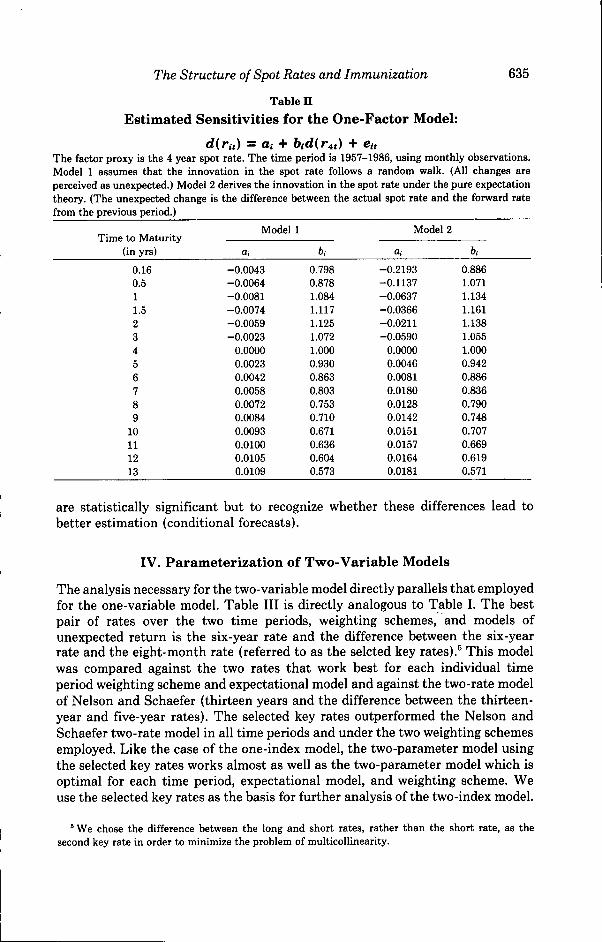
In Table II we present the average intercept (a,) and slope {bt) of the regressionof the unexpected change in different spot rates against the unexpected changein the 4-year spot rate. This is done for both models of unexpected change, andtheir results are quite similar. Note first that the b's not only differ from one(the assumption in the Macaulay measure of duration), but they have a distinctpattern. They start below one, rise above one, and fall to well below one for longrates. While we report in this table only the average results over all six of our 5-year data periods, examination of each 5-year period shows a very similar pattern.

In most previous empirical work where the independent variable was selectedto be the shortest rate in the sample, the sensitivities decline uniformly with thematurity of the spot rate. While it is more convenient to have such a pattern fordeveloping duration measures, the cost, as seen in the previous section, is to haveless explanatory power. Using the four-year spot as the independent variableincreases explanatory power but creates a more complex pattern for sensitivities."

There also appears to be a discernible but less distinct pattern in the interceptswhich implies a nonzero mean in unexpected changes in spot rates. If either ofour two models of estimating the unexpected change in spots were perfectlycorrect, all intercepts should be equal to zero. We can think of four reasons thatcan account for finding nonzero intercepts. The first is the error in variablesproblems. To the extent that the four-year rate is an imperfect proxy for thefactor driving interest rates and that deviations of the four-year rate from thefactor are random, the errors in the independent variable will cause the interceptto be positive and the slope to be lower. The second is the problem of omittedvariables. If the process driving interest rates is really a two-factor model (andwe present evidence later in the paper that it is), one would expect a pattern onthe intercept similar to that found. The third reason is the presence of liquiditypremiums. While this could impact both models, its impact is easiest to see (andshould be larger) for model 2. The presence of the liquidity premium would meanthat the changes in the expected spot rates we derived are overestimates of thetrue expectations. Liquidity premiums change more rapidly for shorter maturitiesthan for long maturities and would result in the pattern of intercepts we found.The fourth reason applies to model 2. It is easy to show that an underestimateof the true thirty-day spot rate would cause the intercept to be negative whenthe dependent variable is a short-term spot rate and positive when it is a long-term spot rate.

We have not tested the statistical significance of the intercepts and slopes, forwe believe that the importance of the presence of an intercept different fromzero and of a slope different from one relates not to whether these differences

* The reason for the more complex pattern is the following. The 6; for any maturity spot is theproduct of the correlation between that spot and the four-year rate and the standard deviation of thespot divided by the standard deviation of the four-year rate. As we move to higher maturities, thestandard deviation of the spot rate uniformly decreases. On the other hand, as we move from verylow maturities to longer maturities, the correlation with the four-year rate increases (reaching amaximum when the maturity is four years) and then decreases. It is this pattern for the two elementsaffecting fe, which accounts for sensitivities at first increasing and then decreasing as we increasematurities.


Table II

Estimated Sensitivities for the One-Factor Model:

din,) = a, + 6,d(r4,) + e.vThe factor proxy is the 4 year spot rate. The time period is 1957-1986, using monthly observations.Model 1 assumes that the innovation in the spot rate follows a random walk. (All changes areperceived as unexpected.) Model 2 derives the innovation in the spot rate under the pure expectationtheory. (The unexpected change is the difference between the actual spot rate and the forward ratefrom the previous period.)

Time to Maturity(in yrs)

0.160.511.523456789

10111213

Model 1

-0.0043-0.0064-0.0081-0.0074-0.0059-0.0023

0.00000.00230.00420.00580.00720.00840.00930.01000.01050.0109

6.

0.7980.8781.0841.1171.1251.0721.0000.9300.8630.8030.7530.7100.6710.6360.6040.573

Model 2

a.

-0.2193-0.1137-0.0637-0.0366-0.0211-0.0590

0.00000.00460.00810.01800.01280.01420.01510.01570.01640.0181

bi

0.8861.0711.1341.1611.1381.0551.0000.9420.8860.8360.7900.7480.7070.6690.6190.571

are statistically significant but to recognize whether these differences lead tobetter estimation (conditional forecasts).

IV. Parameterization of Two-Variable Models

The analysis necessary for the two-variable model directly parallels that employedfor the one-variable model. Table III is directly analogous to Table I. The bestpair of rates over the two time periods, weighting schemes, and models ofunexpected return is the six-year rate and the difference between the six-yearrate and the eight-month rate (referred to as the selcted key rates).^ This modelwas compared against the two rates that work best for each individual timeperiod weighting scheme and expectational model and against the two-rate modelof Nelson and Schaefer (thirteen years and the difference between the thirteen-year and five-year rates). The selected key rates outperformed the Nelson andSchaefer two-rate model in all time periods and under the two weighting schemesemployed. Like the case of the one-index model, the two-parameter model usingthe selected key rates works almost as well as the two-parameter model which isoptimal for each time period, expectational model, and weighting scheme. Weuse the selected key rates as the basis for further analysis of the two-index model.

chose the difference between the long and short rates, rather than the short rate, as thesecond key rate in order to minimize the problem of multicoUinearity.


&I &5 | .S &Ja >o

l l l l l l l lto 0)

x : <x>

2 "5 a,

IIOH >>

^ a_o 00

i

CO ' ^ 0)<U O 3

III

S

ato

S05OIO

d

• "5d

O

m

to toto lO

d d

lO to"O OO 00r-i d

a a^ to

to ^ - I-I ^.•lO .>> .-I .>>

P £̂ «! td

00

d

ato

ghts

a3

x;be

Wei

oE

CO

&0

II

IO

cora

00

•asCO

ao

to

the

c

1c

diff

ere

d th

e

ca_22

r sp

ot

CO

cl

C2

oB

r"•W

CO

yed

i

o

mpl

cl>

CO

a

>̂IO<B

'S• aBCO

'ear

. ^

CO

.s•!.:>

B

s

nee

bet

iffe

re

T30}

:ST3B

rate

a

aCOa

CO

iar

e

CO

0)' • ^

'EH

sa

<2a

J3u

M

mat

uri

tyls

on a

nd

ox:

<u

ates

.

B

BO•pa>• o

B

a

CO

the

' .2

00

a0}

For

lue.

a

as

'Sa

x:

itt

•c3aa

*^.2CO

0)XI

aB

num

ber

i

a.B

.o

te.

a

x:

1a00V

1 in

tl

ior

CO

oB

the

in

CO

inu

ss2'op.(O<u

JS

B

BO

>

oBE

yea:

to

and

the

Sa

pot

1


When different maturity spots were regressed on the selected key rates, therewas a clear pattern to the regression coefficients. While these are modeled laterin the paper, we should note now that the slope coefficients on both rates are notmonotonic with respect to the maturity of the dependent spot rate.

V, Selecting the Best Forecasting Model

In this section we evaluate whether the methods developed in the paper lead tobetter conditional forecasts of the unexpected change in spot rates than docommonly used benchmarks.

A. Alternative Forecast Methods

The analysis to this point has been concerned with determining the best one-and two-index methods to use in forecasting unexpected changes in spot rates.The one-index model (denoted by opt 1 in Table IV) bases forecasts on aunivariate regression where the independent variable is the unexpected changein the four-year spot rate. The two-index model (denoted by opt 2) bases forecastson a bivariate regression where the independent variables are the unexpectedchange in the six-year rate and the difference between the unexpected change inthe six-year rate and the eight-month rate. For each of the models, sensitivitieswere estimated using data for the five years prior to the forecast period.

This way of estimating sensitivities is perfectly feasible as a way of gettingestimates for bond pricing. However, it does not result in a closed-form specifi-cation. For many purposes, a closed-form model is desired. Hence, we constructedand tested two such models. The data analysis from previous sections suggests aform for sensitivities that is quadratic in the natural logarithm of time. Thus, weconstruct regressions of the following form:

bi = co + ciln(i) -I- C2 (ln(i))' + c, (3)

where, bi is the sensitivity of a spot rate of maturity i to an unexpected changein the factor.

This model performed well in fitting the cross-sectional pattern of sensitivities(fe's). The average R^ is higher than .97 for the regression of sensitivities on timein the one-index method and higher than .93 and .99 for the first and secondsensitivities in the two-index model. Forecasts from these models are labeled opt1 s for the one factor smoothed and opt 2 s for the two factors smoothed. Whilethe motivation for this specification is to allow the derivation of a closed-formbond pricing model, its smoothing properties might result in better forecaststhan using the historical sensitivities directly.

We have a number of benchmarks with which to compare our forecasts. Thenatural benchmark is the assumption inherent in Macaulay's duration measure.This measure simply assumes that the sensitivity of all rates to a change in anyrate (including the four-year rate) is one. In Table IV these forecasts are labeledas naive. Our other benchmarks were the models used in Nelson and Schaefer(1983) and Bahbel (1983). Both Babbel and Nelson and Schaefer use the one-year rate in their single-index models, and Nelson and Schaefer use the thirteen-


Table IV

The Out-of-Sample Performance of Competing ModelsModel 1 assumes that the innovation in the spot rate follows a random walk. (All changes areperceived as unexpected.) Model 2 derives the innovation in the spot rate under the pure expectationtheory. (The unexpected change is the difference between the actual spot rate and the forward ratefrom the previous period.) For each model the coefficients are estimated in the prior period. TheMean Square Error is then calculated as a basis of comparison. The models are ranked from best toworst for each subperiod (columns 2-5), and for the overall sample as well (first column).t "Opt 1"is the optimal one-factor proxy, the 4-year rate. "Opt 2" is the optimal two-factor proxies, the 6-yearrate, and the difference between the 6-year and the 8-month rates. "Opt 1 s" is the smoothed one-factor proxy, estimated by equation (3). "Opt 2 s" is the smoothed two-factor proxies, estimated byequation (3). "Naive" assumes that the sensitivities of all rates to a change in any rate are one. "1yr" is the model in which the 1-year spot rate is used as the factor proxy. "13 yrs" is the model inwhich the 13-year spot rate is used as the factor proxy. "13, 5 yr" is a two-state-variables model inwhich the 13-year spot rate and the difference between the 13-year and the 5-year rates are used asthe factor proxies.

1Overall

opt 213, 5 yropt 1opt 1 snaiveopt 2 sl y r13 yrs

1Overall

opt 2opt 1opt 2 s*opt 1 s*naive

2Period 1

opt 2]opt 2 s]13, 5 yropt 1 s]opt 1]13 yrs]naive]l y r

2Period 1

opt 2]opt 2 s]naiveopt 1 sopt 1

Panel A: Model 1

3Period 2

opt 2opt 2 s13, 5 yroptl]opt 1 s]naive]lyr]13 yrs

Panel B: Model 2

3Period 2

opt 2opt 2 sopt 1opt 1 snaive

4Period 3

opt 213, 5 yropt 1opt 1 sl y ropt 2 s*naive*13 yrs

4Period 3

opt 2opt 1opt 1 sopt 2 s*naive*

5Period 4

opt 213, 5 yrnaiveopt 1 sopt 1opt 2 sl y r13 yrs

5Period 4

opt 2naiveopt 2 soptlopt 1 s

* Indicates that the order of these two models is reversed for the cash flow weighting.] Indicates a difference that is insignificant at the 5% level.t The subperiods are 1962-1966,1967-1971,1977-1981, and 1982-1982. The two subperiods (1957-

1961 and 1972-1976) that were used to determine the optimal factors' proxies are excluded since theydo not represent true out-of-sample periods.

year rate and the difference between the thirteen-year and five-year rates in theirtwo-index models. We adopt these rates as additional benchmarks in Table IV,calling them 1 yr, 13 yr, and 13, 5 yr. We use them only for tests of expectationalmodel 1, for this is the framework in which they were proposed by Nelson andSchaefer.

B. Tests

Each of the techniques discussed above is used to prepare forecasts for spotrates in each of four five-year periods. Parameters of all models are estimated


over the previous five-year period. The two five-year periods 1957-1961 and1972-1977 were excluded from the forecasting sample period because they wouldnot constitute a true hold-out sample since they were used to select the indexesthat worked best.^

The methodology used to compare and rank forecast techniques involves testsof differences in mean square forecast errors. More specifically, for each fore-casting technique, squared forecast errors were computed for each maturity. Thiswas repeated each month in the sample period, resulting in a matrix of 60(months) by 31 (maturities) for each forecasting technique. For forecastingmethods taken two at a time, differences between all pairwise entries werecalculated along with a mean standard deviation. In computing the mean andstandard deviation, we used the same two weighting schemes discussed earlier.From the central limit theorem, the differences in forecasts from any twotechniques should be normally distributed, and we tested the significance of thedifferences.

We compare four sample periods as well as combining the four sample periodsinto one, using 240 months. Table IV shows the results when each maturity isweighted equally. The results when they are weighted by their importance inimpacting the change in the bonds portfolio price are identical, except for thosecases that are shown by an asterisk. All differences are significant at the 5%level except where there are brackets indicating insignificance.

C. Empirical Results

From Table IV we can see some definite differences in performance of themethods. The first striking result from Table IV is that, for the overall sampleand in each subperiod, the optimum single-and two-factor proxies we developedoutperformed the proxies utilized by others, including Macaulay's duration model.This would clearly hold in the period where we search for the optimum. However,the results shown in Table IV are for different periods. This consistent outper-formance is evidence that the ranking of preferred proxies for the unknownfactor is sufficiently stable from period to period, so that the procedure discussedin earlier sections leads to better results. The second striking characteristic ofTable IV is the dominance of the two-factor models over their one-factorcounterparts. This dominance holds in each period and for both definitions ofunexpected change in spot rates. Elton, Gruber, and Nabar (1988) also foundstrong evidence of two factors affecting returns.

The third result shown in Table IV is that the smoothed sensitivities under-performed the sensitivities from the prior period. However, the smoothed sensi-tivities outperformed the naive or Macaulay model. Thus, for those who insiston a closed-form solution, there seems to be one that dominates Macaulay's.

* For the periods 1962-1966 and 1972-1981, we tried alternative variations of opt 1 and opt 2. Weexplored the forecasting ability when an intercept was used or left out. We also tested forecastingability when sensitivities and intercepts were calculated for the three 5-year periods and then averagedfor forecasting purposes. These variations were not statistically different from one another, and theirranking varied considerably when we went across the two periods. Using an intercept and just oneprior 5-year period to calculate values performed no worse than any other and was simpler.


However, for most purposes, calculating duration and storing a vector of sensi-tivities are not inconvenient.

The last result that needs to be highlighted is the overall performance of thenaive or Macaulay measure. Previous literature has shown that this measure hasnot been easy to beat. However, in our tests, both the one-variable and two-variable optimum models always outperform Macaulay's measure. Moreover, forexpectational model 2, it was the poorest performer, and, for expectational model1, it outperformed the smoothed two-variable method and two benchmark one-variable models.^

In summary, our technique for choosing the optimal proxy worked well withboth one- and two-variables models. Overall, the two-variables model outperformsthe one-variable model, and all outperform benchmark models.

VI. Conclusion

Empirical work on bond pricing needs to assume something about the relationshipbetween unexpected spot rate changes of different maturities. In the mostcommon approach, unexpected changes in all spot rates are described by changesin one or more key spot rates. While previous studies have chosen these factorsin an ad hoc manner, this paper shows how to select the factors and structurewhich best describe the correlations across unexpected changes in spot rates.

In fact, our findings indicate that the four-year rate serves as the best proxyin the one-state-variable model, while the eight-month and six-year rates do bestin the two-state-variables model. Also, we find that the two-factor model outper-forms the one-factor model. Our model produces out-of-sample predictions su-perior to those using Macaulay's duration model and those using other statevariable proxies. These results may explain why models used in the area ofimmunization, which assume complex relationships between changes in spotrates, have not, in general, outperformed the simplest immunization model putforth by Macaulay: the inferior results may be due to an inappropriate choice offactors describing the unexpected changes in spot rates.

A deeper understanding of the structure of unexpected changes in spot rates isof fundamental importance as an aid to understanding risk in the bond markets.Thus, our results may be used in the pricing of debt instruments, the pricing ofoptions on debt instruments, the construction of bond portfolios, and perform-ance evaluation of bond portfolios.

' We performed one other set of tests. We added the errors at each point in time across thematurities, weighting each maturity equally or weighting according to their importance in pricesensitivity. This allows cancellation of errors. If errors are random, then allowing overestimates forthe maturity to cancel with underestimates for second maturity will produce a better measure of thesensitivity of price to an unexpected change in interest rates. However, there is a second pattern. Inthis pattern the sign is very much a function of maturity: short maturities having positive residualsand long maturities having negative residuals, or vice versa. Hence, this technique is very sensitiveto the choice of the longest maturity. A bond with a maturity different from 13 years would performvery poorly because the errors would not tend to cancel out. Thus, the results of Table IV are morereflective of true relative performance.


Appendix A

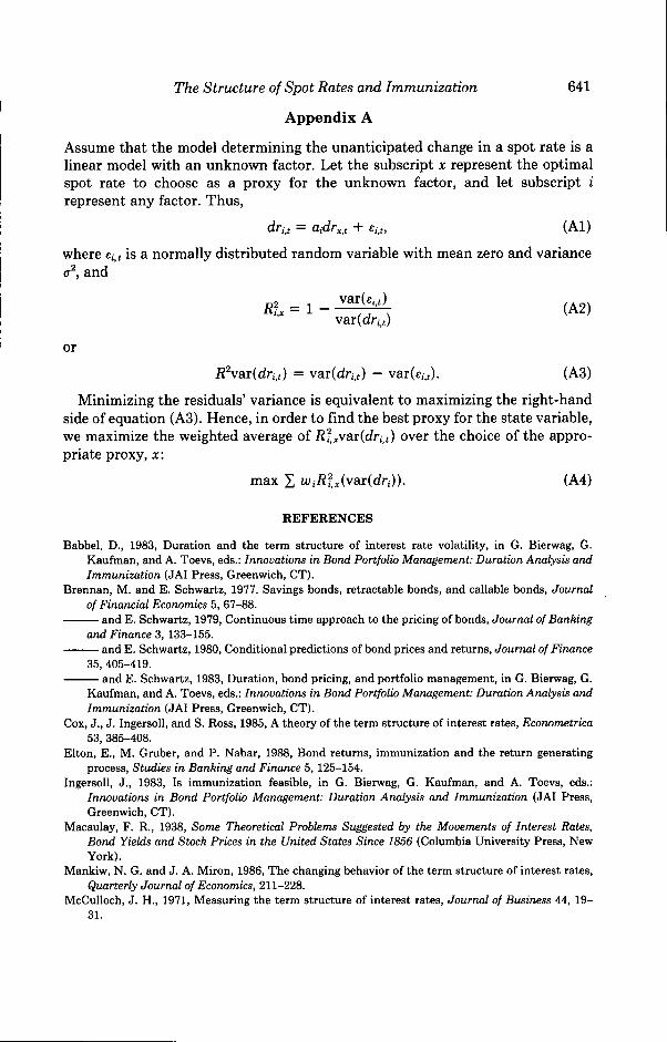
Assume tbat the model determining the unanticipated cbange in a spot rate is alinear model witb an unknown factor. Let the subscript x represent the optimalspot rate to choose as a proxy for tbe unknown factor, and let subscript irepresent any factor. Tbus,

+ ei,t, (Al)

wbere £;,( is a normally distributed random variable witb mean zero and variance(7̂ , and

RI = 1 - I ^ (A2)

var(dri,()

or

i,t). (A3)Minimizing the residuals' variance is equivalent to maximizing the right-band

side of equation (A3). Hence, in order to find tbe best proxy for the state variable,we maximize the weigbted average of i??,xvar(dri,() over tbe cboice of the appro-priate proxy, x:

max I WiRlAyaHdn)). (A4)

REFERENCES

Babbel, D., 1983, Duration and the term structure of interest rate volatility, in G. Bierwag, G.Kaufman, and A. Toevs, eds.: Innovations in Bond Portfolio Management: Duration Analysis andImmunization (JAI Press, Greenwich, CT).

Brennan, M. and E. Schwartz, 1977. Savings bonds, retractable bonds, and callable bonds. Journalof Financial Economics 5, 67-88.

and E. Schwartz, 1979, Continuous time approach to the pricing of bonds. Journal of Bankingand Finance 3, 133-155.

and E. Schwartz, 1980, Conditional predictions of bond prices and returns, Joumal of Finance35, 405-419.

• and E. Schwartz, 1983, Duration, bond pricing, and portfolio management, in G. Bierwag, G.Kaufman, and A. Toevs, eds.: Innovations in Bond Portfolio Management: Duration Analysis andImmunization (JAI Press, Greenwich, GT).

Cox, J., J. Ingersoll, and S. Ross, 1985, A theory of the term structure of interest rates, Econometrica53, 385-408.

Elton, E., M. Gruber, and P. Nabar, 1988, Bond returns, immunization and the return generatingprocess. Studies in Banking and Finance 5, 125-154.

Ingersoll, J., 1983, Is immunization feasible, in G. Bierwag, G. Kaufman, and A. Toevs, eds.:Innovations in Bond Portfolio Management: Duration Analysis and Immunization (JAI Press,Greenwich, GT).

Macaulay, F. R., 1938, Some Theoretical Problems Suggested by the Movements of Interest Rates,Bond Yields and Stock Prices in the United States Since 1856 (Columbia University Press, NewYork).

Mankiw, N. G. and J. A. Miron, 1986, The changing behavior of the term structure of interest rates.Quarterly Journal of Economics, 211-228.

McGuUoch, J. H., 1971, Measuring the term structure of interest rates. Journal of Business 44, 19-31.


, 1975, The tax adjusted yield curve, Journal of Finance 30, 811-830.Nelson, J. and S. Schaefer, 1983, The dynamics of the term structure and alternative portfolio

immunization strategies, in G. Bierwag, G. Kaufman, and A. Toevs, eds.: Innovations in BondPortfolio Management: Duration Analysis and Immunization (JAI Press, Greenwich, CT).

Richard, S., 1978, An arbitrage model of the term structure of interest rates. Journal of FinancialEconomics 6, 33-37.

Vasicek, O., 1977, An equilibrium characterization of the term structure. Journal of FinancialEconomics 5,177-188.

Documents

The Structure of Spot Rates and Immunizationforum.johnson.cornell.edu/faculty/michaely/The Structure of Spot...THE JOURNAL OP FINANCE • VOL. XLV, NO. 2 • JUNE 1990 The Structure