The Structure of Ocean Transport Charges · Several empirical models of international trade flows, ... neighborhood of .50. ... chiefly value at the point of shipment,

This PDF is a selection from an out-of-print volume from the NationalBureau of Economic Research

Volume Title: Explorations in Economic Research, Volume 1, Number1

Volume Author/Editor: NBER

Volume Publisher: NBER

Volume URL: http://www.nber.org/books/expl74-1

Publication Date: 1974

Chapter Title: The Structure of Ocean Transport Charges

Chapter Author: Robert E. Lipsey, Merle Yahr Weiss

Chapter URL: http://www.nber.org/chapters/c4891

Chapter pages in book: (p. 162 - 193)

3ROBERT E. LIPSEYQueens College and National Bureau

of Economic Research

MERLE YAHR WEISSTemple University and National Bureau

of Economic Research

The Structure of Ocean TransportCharges

ABSTRACT: This paper attempts to estimate the commodity structureof ocean transport charges: the relation between the characteristics ofcommodities and the charges for shipping them. The purpose is toprovide a method of estimating such charges for use in models ofworld trade, to explain which goods will enter international trade, andhow much trade will take place in the commodity in general andbetween particular countries. Because comprehensive transport pricedata are not available we have used actual charges for individualshipments to construct a model of commodity differences inrates. ¶ We find that the main determinants of rates, which make upour estimating equation, are the value per ton of a commodity, itsbulkiness (cubic ft. per ton), the distance over which it is shipped, theprevalence of small individual shipments, and the possibility of ship-ping the product by tanker. We found no evidence that rates onexports from the United States were higher than on exports of otherdeveloped countries, once commodity and route characteristics weretaken into account. There was some weak evidence that productsshipped mostly by liner carried relatively high charges and that anexport surplus on a shipping route led to lower rates on imports thanon exports.

162

Structure of Ocean Transport Charges 163

INTRODUCTION

This paper1 attempts to give some empirical content to the idea of acommodity structure of ocean transport prices that helps to determinewhich goods will enter international trade, what proportion of the totaloutput of a commodity will be traded, and which countries will beexporters and which will be importers of each commodity. There are nocomprehensive, publicly available data on actual transport charges ininternational trade.2 Requiring such information as an element in theexplanation of the pattern of trade, by commodity, we have attempted toquantify the main factors underlying commodity differences in the price oftransport and thus to provide a method of estimating the price of oceantransport for each commodity. We have done this by examining twobodies of data on actual transport charges and generalizing from them, aswell as we can, about the determinants of these charges. However, wewere not primarily interested in the factors determining the level of oceantransport charges or changes in that level over time, differences amongroutes or among ports, or the effect of shipping conferences on rates.

Several empirical models of international trade flows, attempting toexplain the volume of total trade between two countries, have useddistance as a proxy for various barriers to trade, of which transport cost isone. A study by Tinbergen, for example, explained the size of the tradeflow between any two countries by the GNP of each and the distancebetween them, assuming that distance was a rough measure of transportcost, although it could also stand for an index of the amount of informationon export markets.3 Distance proved to be a significant variable, with theappropriate negative sign in almost all of his equations.

Linneman, in a much more elaborate study that included income,population, and several variables for various preferential trading arrange-ments, also found distance to be an important and significant negativeinfluence on the amount of trade between countries.4

Several other similar models of trade based at least partly on distance,but including other variables such as income, membership in preferentialmarket areas, and the total level of each country's exports and imports,have been described by Taplin and by Learner and Stern.5 The onlyinstance we found of an attempt to introduce cost rather than distance wasin a study by Beckerman in which a crude ordering of country pairs by thecost of transportation between them, based on differences between expor-ters' valuations (excluding transport and insurance charges) and importers'valuations (including transport and insurance charges), was used to explaintrade patterns within Europe.'

164 Robert E. Lipsey and Merle Yahr Weiss

DETERMINANTS OF THE PRICE OF TRANSPORT—THEORETICAL CONSIDERATIONS

Most theoretical explanations of the structure of ocean transport chargesdeal with supply elements, listing the factors that determine the cost ofproducing these services. Some of these relate to commodity characteris-tics and others to characteristics of particular shipping routes. We aremainly interested in the former but we have attempted to introduce thelatter, where possible, to insure that their presence will not bias ourestimates of the effects of the commodity characteristics.

Among the commodity characteristics are the stowage factor (that is, thenumber of cubic feet of shipping space taken up by one ton of acommodity); the possibilities of shipping the product in bulk usingspecialized vessels, or for using tramp rather than liner shipment; the easeof loading or unloading; the fragility of the product or its susceptibility todeterioration; and the average size or shipping weight per shipment. Sizeof shipment is important because small shipments require additional laborcosts, such as extra handling, for a given amount of weight.

Among the route characteristics are the distance of shipment, the costs ofloading and unloading in particular ports, the degree of competitionamong shipping lines, and the extent of any imbalance of trade betweenoutbound and inbound sh4pments.' The significance of the last factor isthat it might cause severe competition for freight, and therefore lowercharges, in the direction of less trade.

If the shipping industry were perfectly competitive and we were willingto treat shipping services as homogeneous, at least within liner or tankershipping, we could ignore demand factors, since we are interested prima-rily in the structure of rates at one time rather than in changes over time.However, it is well known that the unit value (value per ton) of thecommodity to be shipped is an important determinant of ocean transportcharges. It is difficult to explain a strong positive relationship between theunit value of commodities and transport charges per ton by any costfactors. The only clearly positive relationship between the unit value andthe cost of producing transport services is based on the cost of insurance,which is included in our measure of transport cost. Insurance cost mayappear either as a specific payment or as the need for stronger guaranteesof the quality of service necessary to obtain the business of shippingvaluable commodities. However, the cost of insurance is only a small partof transport cost, and since it depends on many factors other than unitvalue, one would not expect the relationship between unit values andinsurance cost to account for a large part of the variability of transportcharges. In fact, evidence from the United Nations' Latin American freightrate study,8 referred to below in the section on comparisons with other


results, indicates that insurance charges could account for no more than.02 or .03 of unit value coefficients which we found to be in theneighborhood of .50.

If shipping is subject to monopolistic pricing, mainly through the opera-tion of shipping conferences and barriers to entry, a positive relationshipbetween unit values and transport charges could result from price dis-crimination since the demand for transport services is likely to be moreinelastic for higher-valued commodities than for cheaper ones. That is, ifone commodity is more expensive per ton than another, a given rise intransport cost per ton will add less in percentage terms to its price than tothat of the cheaper product. If the elasticity of final demand is the same forboth commodities, then sales, and therefore the purchase of transportservices, will decline less for the more expensive product. Thus, theelasticity of the derived demand for transport services will be lower for theexpensive product, and the difference in the elasticities provides theopportunity for discriminating carriers to charge higher freight rates on themore expensive products.

Our model of the determination of transport charges in a cross-section ofcommodities and trade routes therefore assumes that these charges are afunction of a variety of cost elements on the supply side and of theelasticity of demand for ocean transport, the unit value of the commoditybeing the determinant of the demand elasticity. To our data on transportcharges for particular shipments we have thus fitted equations using unitvalue and several other characteristics of commodities and those of traderoutes. The basic data are from a Census Bureau study of the differencesbetween two methods of valuation for U.S. imports: the official valuations(those reported on customs documents, chiefly value at the point ofshipment, excluding freight and insurance) and the value at the point ofentry into the United States, including freight and insurance. The differencebetween these two values, with some adjustments, is our measure oftransport charges. Supplementary data, referred to hereafter as "biddingdata" and used as a check on the Census data, are from an earlier NationalBureau study of international price competitiveness. Both data sets aredescribed more fully in the appendix. Since the Census data are broader incommodity coverage, they are the basis for most of the conclusions thatfollow.

TRANSPORT PRICE ESTIMATING EQUATION

The basic estimating equation for the price of transport, based on Censusdata for U.S. imports, treats the transportation charge per ton as a functionof the unit value, the distance shipped, the stowage factor for the commod-


ity, a dummy variable for products that are at least to some extent shippedby tanker, and a dummy variable for small shipments, which we define asshipments under one ton in weight. All the coefficients for these variableswere statistically significant at the 5 per cent confidence level and all hadthe signs that would be expected. Some other variables that were tested,but not finally accepted for the estimating equation, are discussed below.

The estimating equation,9 with all variables in logarithmic form, is:

(1) FR = —3.53 + .52UV + .30D1 + .35ST + .3OSW — .51TA(57.35) (13.51) (18.18) (6.22) (12.25)

R2=81

where FR is the transport charge (in $ per ton), UV is unit value ($ per ton),0! is distance (nautical miles), ST is stowage (cubic feet per ton), SW is adummy variable for a shipment of less than one ton, and TA is a dummyvariable for a product that was in some instances imported by tanker.Figures in parentheses are t-values for the coefficients.

The equation states that a long distance from origin to destination,bulkiness (volume per ton), and smallness of a shipment all add to theprice of transport per ton, presumably by raising the cost. The feasibility ofshipment by tanker reduces the price. High value per ton raises the price oftransport, and this is the strongest relationship of all.

The degree of our success in matching the actual determinants oftransport charges can be seen in Table 1, which compares the ratesestimated from equation (1) with the reported charges for those StandardInternational Trade Classification (SITC) groups in which we had at leastthirty observations. Some wide discrepancies are evident, and for a few ofthem explanations come readily to mind. For example, we have novariable to take account of fragility or likelihood of damage in shipment,except to the extent that value per ton serves as a proxy for thesecharacteristics; and that omission probably accounts for the underestimatesof transport charges on glassware and pottery and possibly for those onalcoholic beverages and toys and games.

For some purposes interest in transport costs is centered not on thefreight rate (cost per ton) but on the freight factor: the ratio of total freightpayments to the total value of the shipment. The freight factor may be abetter measure than the freight rate of the influence of transport costs as abarrier to trade and would be useful also for estimating aggregate transportcosts if value data, but not tonnage data, were available.

An equation for freight factors could presumably be estimated directly,but in these logarithmic equations, freight rate and freight factor equationsare both linear, differing only in one coefficient.

TABLE 1 Reported and Estimated a Transport Charges: Averages byCommodity Groupsb (dollars per metric ton)

Average of Average ofReported Estimated

SITCC Charges Charges

011 Meats, fresh, frozen, etc. 87 66013 Meats in containers, meat prep., etc. 50 64031 Fish, fresh, frozen, etc. 69 65051 Fruit, fresh, and nuts, fresh or dried 24 27061 Sugar and honey 8 10071 Coffee 40 52081 Feeding-stuff for animals 25 20112 Alcoholic beverages . 64 50231 Crude rubber 51 44262 Wool and other animal hair 90 103281 Iron ore and concentrates 2 2

283 Ores and concentrates, non-ferrous 5 4

331 Petroleum, crude and partly refined 2 3

332 Petroleum products 2 2

422 Fixed vegetable oils, exc. soft 1 5 29512 Organic chemicals 31 30631 Veneers, plywood board, etc. 39 34653 Textile fabrics, woven, exc. cotton 87 105664 Glass 33 29665 Glassware 173 87666 Pottery 92 60674 Iron and steel plates and sheets 19 14

132 Road motor vehicles 130 109841 Clothing 254 260851 Footwear 196 171

861 Scientific, medical, etc., Inst. and appar. 319 311

894 Toys, games, sporting goods, etc. 270 . 189• 899 Manufactured articles n.e.s. 201 169

• aEstimated from equation (1).bAverages are geometric means.cAll groups with thirty observations or more. Some of the SITC titles are abbreviated here.

Thus, if the freight rate equation is

log FR = a + b log UV + c log DI + d log ST

implying, in arithmetic form:

FR = aUV1'


the freight factor equation is

log FF = a + (b — 1) log UV + c log DI + d log ST

implying, in arithmetic form,

FF = DIC STa

and our estimating equation for freight rates can easily be transformed intoan estimating equation for freight factors. This is, in fact, how we derivedthe freight factor equation used for Table 2, which lists the actual andestimated freight factors. We can use these estimated transport costs ofindividual commodities as a variable to explain trade flows or, as analternative, we can use them to turn price relationships among exportingcountries at the point of export, excluding transport charges, into deliveredprice relationships, including transport charges. A number of studies haveused export unit values to represent prices of exporting countries,10 andsome more recent work has involved the calculation of actual price levelsfor goods offered in international trade.h1 In both cases the comparisonsinvolve prices exclusive of transport charges. However, one would expectthat purchase decisions are based on delivered prices, so that equal U.S.and U.K. export prices, for example, would mean that the U.S. suppliesCanada but the U.K. supplies Ireland.

The equations derived in this paper permit the analyst to transform pricesor price ratios excluding transport charges into delivered prices or ratiosapplicable to individual markets by inserting the appropriate values for theindependent variables. Even if no relative price data exist, the freightfactors derived from these equations provide estimates of that part ofdifferences in relative delivered prices that could be accounted for bytransport charges, if these costs are borne by purchasers. Thus if weassumed that prices from different suppliers to one market were identicalbefore transport charges were added, w could estimate the relative differ-ence in delivered prices between one supplier and another. If we assumedthat delivered prices in a market were identical, we could estimate relativedifferences in prices at the point of shipment.

TESTS OF THE ESTIMATING EQUATION

Comparisons with Bidding DataSince the structur of transport charges in U.S. import trade, to which theCensus data relate, could be quite different from that on other trade routes,we. are fortunate to have a completely independent ource of data, fordifferent years and different routes, with which we can compare the results

TABLE 2 Reported and Estimateda Freight Factors: Averagesby Commodity Groups (percentage ofvalue of shipment)

Average ofReported

Average ofEstimated

Freight FreightSITCb Factors Factors

01 1 Meats, fresh, frozen; etc. 11 8

013 Meats in containers, meat prep., etc. 4 5

031 Fish, fresh, frozen, etc. 7 6

051 Fruit, fresh, and nuts, fresh or dried 13 15

061 Sugar and honey 7 8

071 Coffee 5 6

081 Feeding-stuff for animals 18 14

112 Alcoholic beverages 9 7

231 Crude rubber 13 11

262 Wool and other animal hair 5 6

281 Iron ore and concentrates . 26 29283 Ores and concentrates, non-ferrous 14 11

331 Petroleum, crude and partly refined 15 19

332 Petroleum products 14 16

442 Fixed vegetable oils, exc. soft 6. 11

512 Organic chemicals 4 4

631 Veneers, plywood board, etc. 16 14

653 Textile fabrics, woven, exc. Cotton 6 7

664 Glass 14 12

665 Glassware 11 6

666 Pottery 12 8

674 Iron and steel plates and sheets 11 8

732 Road motor vehicles 9 7

841 Clothing 5 5

851 Footwear 7 6

861 Scientific, medical, etc., inst. and appar. 2 2

894 Toys, games, sporting goods, etc. 9 6

899 Manufactured articles n.e.s. 9 8

aEstimated from equation (1).bAll groups with thirty observations or more. Some of the SITC titles are abbreviated here.

from the Census data. The equation from bidding data, which coveredexports by the United States and other developed countries mainly toless-developed countries, particularly in Latin America, during 1 953—64,was

(2) FR = —4.95 + .7OUV + .34D1 + .5OST R2 = .59(28.23) (6.93) (13.08)


The variables for small shipments and tanker shipment do not appear inthis equation because no such shipments were included in these data. Theother three variables were statistically significant, as in the Census data,and had the same sign. However, the coefficients were all higher in thebidding data, .70 against .52 for unit value, .34 against .30 for distance,and .50 against .35 for stow'age.

We pooled the two sets of data to test whether the level and the structureof rates implied by the bidding data were significantly different from. thosederived from Census data. An equation containing only a dummy variablefor bidding data, implying that the other coefficients were assumed to beidentical in the two sets of data, was (in logs):

(3) .FR = —3.61 + .53UV + .37ST + .3001 + .275W — .48TA(63.71) (21.26) (14.80) (5.96) (12.15)

+ .67B R2 = .81

(23.52)

where B is a dummy variable for bidding data and .the other variables arethose defined for equation (1). The level of rates, on the a sumption that thecoefficients for UV and other variablesare identical in the two data sets, issignificantly higher in the bidding data than in the Census data. However,the other coefficients can be tested by inserting cross-product variables,multiplying B by each of the others. The cross-product term for distancedid not appear to be significant and was dropped, leaving as the resultingequation:

(4) FR —3.56 + .52UV + .355T + .3 101 + .305W — .51TA(60.46) (19.14) (15.24) (6.57) (12.89)

— 1.11B + .17(B x UV) + .14(B x ST) R2 = .81(4.11) (5.41) (2.77)

which implies that both the unit value and the stowage coefficients weresignificantly higher in the bidding data than in the Census data, whereasthe constant term was significantly lower.

The bidding data thus confirm the choice of variables but suggestdifferent values for some coefficients. A number of possible interpretationsof these differences are discussed below.

Tests with Independent Unit Value Data

A basic problem in our estimating equation is that the freight rate and theunit value are both variables that have the weight of the shipment in theirdenominator; that is, freight rate is computed by dividing the total freightcost by the weight of the shipment, and unit value is computed by dividing


the total value of the shipment by the weight of the shipment. If there weresignificant errors of measurement in the weight variable, they could havebiased both the unit value coefficient and the correlation measure. Theextent of the bias would depend on the characteristics of the errors; forexample, the correlation between the errors and the true values of thevariables. To check for possible bias from this source, we coflectedpublished value and quantity data and calculated independent unit valuesfor the commodities and countries in our transport charge data, as de-scribed in the appendix, matching the SITC categories in our transportcharge data to those of the published value and quantity data. The numberof independent unit values was, of course, smaller than the number of ouroriginal observations because the independent unit values representedwhole commodity groups rather than individual shipments.

We then calculated regressions with the logarithms of the independentunit value, distance, and the stowage factor as independent variables, aswell as, in the Census data, dummy variables for small weight and tankershipment, and the logarithm of the transport charge as the dependentvariable. These results are compared with the original equations in Table312

We were concerned that our unit value coefficient obtained from thewhole data set might be biased by errors in the measurement of weight, butas noted in Table 3, the magnitudes and signs of these coefficients basedon the two sets of unit value observations are very similar. In the Censusdata the unit value and distance coefficients are almost unaffected by thesubstitution of the independent unit values (they change from .52 to .50and .30 to .32) and the stowage coefficient is unchanged. Only the smallshipment and tanker coefficients are altered substantially. The small ship-ment coefficient may pick up some of the variation artificially excludedfrom the unit value variable because. the unit values from the publisheddata, matched only to the country and commodity of each freight rate, areidentical for several observations.

The bidding-data coefficients change more significantly, the coefficientsfor unit value and stowage declining and becoming closer to those fromthe Census data and that for distance increasing and differing by more thanoriginally from the Census results. We suspect, from the change in the unitvalue coefficient, that some bias from measurement errors may have beenpresent in the initial result. It is not surprising that the bidding data weremore subject to this defect because many of the shipping weights wereestimated, whereas those used for the Census equations were part of theoriginal data set.

The adjusted R2 decreased in each case, as we would expect, since wesubstituted the average unit value of a commodity group for unit valuesspecific to individual shipments. In this way we ignored some known

TABLE 3 Comparison between Regression CoefficientsBased on Original Unit Values and CoefficientsBased on Independent Unit Values

Equation Intercept UV ST UI SW TA R2

Census Data

(1) —3.53 .52(57.35)

.35(18.18)

.30(13.51)

.30(6.22)

—.51

(12.25).81

(5) —2.34 .50(42.33)

.35(15.29)

.32

(12.50)

.72

(13.53), —.57

(11.82).75

(2) —4.95 .70(28.23)

Bidding

.50(13.08)

Data

.34(6.93)

. .59

(6) —4.30 .68(26.38)

.49(12.29)

.28(5.12)

.58

(7) —4.93 .58(19.64)

.44(9.56)

.45(7.33)

.47

(1) Original data, 2,889 observations.(2) Original data, 835 observations.(5) Independent unit values.(6) Original data for which matching independent unit values were available, 756 observations.(7) Independent unit values.

variation in the independent variable that we knew was associated withsome of the variation in the dependent variable.

On the whole, then, the Census-data equations passed this test quitesuccessfully, and we feel fairly safe in proceeding on the assumption thatthe problem of biased coefficients is negligible in the Census data and is ofsome, but not major importance, in the bidding data.

Non-Linearity and Heteroscedasticity

We have fitted linear equations in logs although there is no strongtheoretical basis for the linear form. The recent UNCTAD study, describedmore fully below, used linear arithmetic equations that we found toproduce a much poorer fit and unstable coefficients. It is quite possible, ofcourse, that a more complex function would give a still better fit than thelog linear function, and to examine that possibility we tested the estimatingequation for signs of non-linearity. The method was to split the sample inhalf according to the ranking of several variables, asking, first, whether thecoefficient for a variable among the observations with larger values for thevariable was significantly different from the coefficient among the observa-tions with smaller values, and second, whether coefficients for indepen-


dent variables differed significantly between commodities carrying lowertransport charges and those bearing higher rates. The most convenient wayto perform the tests was to assign a dummy variable to that half of eachdistribution which contained the larger observations and introduce into theequation cross-product terms between that dummy variable and eachindependent variable. Thus, for example, if we defined LU as the dummyvariable for large unit value (that is, higher than the median unit value), weintroduced a term (LU) (UV) into the equation. A positive and statisticallysignificant coefficient for (LU) (UV) would indicate that a given percentagedifference between two unit values was associated with a larger percentagedifference in freight charges among more expensive goods than among thecheaper products.

The results of these tests, summarized in Table A3 in the appendix,suggest that there were some statistically significant differences incoefficients, but that permitting slopes to vary in the two halves of thedistributions would, in most cases, produce little improvement in the fit ofthe equation and change the coefficients only slightly.

The separation by size of unit value (equation 26) has comparativelylittle effect on the coefficients but indicates that a given percentage changein unit value adds less to the freight charge at higher unit values than atlower ones. The breakdown by stowage factor (equation 27) suggests thatthe impact of bulkiness on freight rates is greater among bulky com-modities than among less bulky ones. The distance breakdown (equation28) indicates that the effect of a given percentage change in distance issmaller among long voyages than among short ones. In none of these casesdid the addition of the dummy variable raise the R2 substantially, eventhough all the dummy variables were statistically significant at the 5 percent level.

A greater effect on the coefficients was produced by separating the groupinto high and low transport rates, the dependent variable (equation 29).The higher R2 is meaningless since transport cost was, to some extent,being placed on both sides of the equation. The equation does suggest thatstowage affected transport charges much more among commodities withhigh rates than among those with low rates.

One reason for the differences in coefficients that appear when observa-tions are divided into transport rate groupings is suggested by our tests forheteroscedasticity. Wetested for heteroscedasticity, using Bartlett's test anda four-way division of the observations, with orderings by transport charge,unit value, stowage, and distance. The latter two orderings did not producea rejection of the hypotheses of homoscedasticity at the 5 per cent level,the unit value ordering indicated a rejection at the 5 per cent level but notat the 1 per cent level, but the ordering by transport charges produced verystrong evidence of heteroscedasticity. It may be, then, that the differences


in coefficients between high- and low-transport charge groups reflect thisheteroscedasticity rather than any true non-linearity in the relationships.

Some Experiments with the TransportPrice Equations

Since the bidding data cover a period of several years, we could presuma-bly use them to measure changes in the structure of transport prices,although the observations become fairly thin when they are divided byperiods of time. If we fit an equation (in logs) to the bidding data for1959—61 and 1962—64 using a dummy variable, E, for observations for1959—61, and adding the cross-product terms for 1959—61 for each vari-able, we obtain:

(8) FR = —2.89 + .69UV + .4OST + .140! — 2.81E + .08(E x UV)(15.85) (5.83) (1.53) (2.64) (1.46)

— .03(E x ST) + .29(E x DI) = .60(.40) (2.63)

The equation implies that there was no unambiguous. shift in the level ofrates, since the coefficient for E is negative; but the cross-product terms forunit value and distance are positive. It would be possible to calculate theimplied transport charges for different types of commodities in the twoperiods and to weight these in any proportions considered appropriate toproduce an index of transport charges.

Another possible source of information on changes in transport chargesis the comparison between bidding- and Census-data equations, since thebidding data referred to an earlier period. The equation with only a singledummy variable for bidding data showed a considerably higher level forthe earlier period. The more complete equation was also more ambiguous,since the dummy variable for bidding data was negative, although thecross-product terms for the unit value and stowage coefficients werepositive. The two equations suggest that although the level of transportcharges was probably lower in general in the Census data, there might besome products, with low unit value and low storage factors, for which theCensus data equation implied higher charges.

There are several possible reasons for the difference in level betweenequations for the two data sets, since the bidding data differ from theCensus data in several respects other than just the method of collection.One is that the Census data relate entirely to U.S. imports, whereas thebidding data cover mainly shipments from the United States and otherdeveloped countries to less-developed countries, particularly in LatinAmerica. Another is that the bidding data cover mostly the years 1960—64,but the Census data are all for 1966. Still a third difference is that the


Census data cover a much larger number and variety of commodities thanthe bidding data.

A possible explanation of the difference is that transport charges de-clined between the early 1960s and 1966, in the sense that in 1966 theywere lower than the levels implied by the bidding-data equation; takingaccount of unit value, distance, and stowage factors. If transport chargesper ton for each commodity on each trade route increased, but not somuch as our equation predicted, given a rise in unit values, we wouldconsider that transport charges had fallen.

There are at least two alternative explanations for the difference betweenthe two transport charge levels: (1) that transport charges into the UnitedStates are lower, given the commodity characteristics of trade, than thoseon shipments out of the United States and out of other developed coun-tries, or at least lower than on those countries' shipments to Latin America;(2) that the amount of discrimination by shipping firms, as indicated by theextent to which they charged higher rates for more valuable commodities,was greater in the earlier period than later, or greater on the exports of theUnited States and other developed countries, at least those to LatinAmerica, than on U.S. imports.

These data thus do not rebut the claim that transport charges favor U.S.imports as compared to U.S. exports, but because of the differences intiming and commodity coverage between the sources we cannot draw anyfirm inference on this issue. A related claim that transport charges on U.S.exports are higher than on the corresponding exports by other countries isnot supported by a test in which the bidding-data dummy variable used forequation (3) is replaced by separate variables for U.S. exports and exportsby other countries. The coefficients for the two origins of exports arealmost identical, a fact that suggests that transport charges, taking accountof product mix, were not significantly different.

A factor not included in our equations is the possibility of shipping aproduct other than the tanker products by some method other than liner,including the use of specialized bulk cargo vessels or tramp ships. Severalversions of this variable were tried: the percentage of tonnage shipped byliner, a dummy variable if any of the product was imported by non-liner(other than tanker) shipment, and a dummy variable for products of whichmore than 10 per cent of imports was by non-liner shipment. Thesevariables had the expected sign: positive for percentage shipped by linerand negative for the two dummy variables. However, none of thecoefficents was statistically significant at the 5 per cent level and wetherefore omitted these variables from the basic estimating equation. Anexample of one of these coefficients is given in equation (9), where NL is adummy variable for a commodity of which non-liner imports were 10 per,cent or more of total imports into the United States. If one takes the


coefficient at face value, it seems to imply, as one might expect, thatshipment by tramp steamer or other non-liner mode is cheaper than byliner or that the possibility of such shipment lowers even the liner rates forthe affected products.

(9) FR = —3.47 + .52UV + .35ST + .30D1 + .3OSW — .54TA(54.83) (18.08) (1 3.49) (6.25) (11.97)

— .O5NL R2 = .81(1.70)

It has also been suggested that transport charges are affected by thebalance of tonnage on a route. The hypothesis is that, if outboundtonnage exceeds inbound tonnage on a route, outbound rates will becomparatively expensive and inbound rates will be cheap, as the surplusof capacity for inbound shipping induces price-cutting among carriers.Using some data on shipments along particular trade routes, we classi-fied origin-destination combinations into twenty-seven routes and calcu-lated the ratio of export tonnage to import tonnage and the differencebetween them for each route. The coefficients for the balance onliner shipment, non-liner shipment, and both combined proved of nostatistical significance in any of the equations we tried, and oftenhad the wrong sign. However, a cross-product term for (NL)

(where XNL

is the ratio of non-liner exports to non-liner imports on a

trade route, although it was not significant at the 5 percent level, did havea t-value greater than 1 and the expected negative sign, as in equation (10).

(10) FR —3.55+ .52UV + .355T + .3W! + .305W — .53TA(56.69) (18.17) (13.59) (6.22) (12.31)

— .006(NL)( XNL R2 = 81(1.51) k MNL /

If the coefficient is taken as given, it implies that an export surplus onnon-liner trade on a route lowers the transport charge for non-liner importson that route. The relationship is not strong, but it is in the expecteddirection and does give some support to the role of the trade balance.

COMPARISON WITH OTHER FINDINGS

Our results agree with earlier studies13 in identifying the unit value as themost important determinant of freight rates. However, none of theseauthors calculated any coefficients for the other variables we include andfind to be significant, or estimated a significant, specific relationship


between freight rates and unit values. With better data we are able toestimate the separate influence of distance, stowage, and size of shipmenton freight rates, Furthermore, our results suggest that the omission of any ofthese variables may cause the others to be miscalculated, as there issignificant and positive correlation between unit values and distance andbetween unit values and stowage factors. That omission of variables mayaccount for the difference between our estimate of the unit valuecoefficient and those calculated by Moneta, which ranged between .23and .29. However, other explanations for the difference are possible. TheMoneta data were calculated from grouped observations rather than fromindividual shipments, the distance variable was taken into account in acrude manner by dividing the observations into five exporting areas, andthe data referred to a period much earlier than ours.

Benjamin Chinitz, in a 1956 study, examined the freight rate structure oftwo conferences that had published rates covering commodities exportedfrom the United States to His major purpose was to investigatewhether conference rates implied rate discrimination in ocean transport.Holding constant the stowage factor, he found the correlation between thepublished conference freight rate and the unit value for each commodity tobe quite low, and thus unlike the strong relation in our equations.

The most elaborate study of the structure of transport charges is a recentECLA volume on transport charges for exports from Latin America.15 Thedata are quite different from ours, the rates being derived from conferencetariffs and thus confined to liner trade and to official rates. The approachwas also different, separating the elements of transport charges into twocomponents. One was what the authors referred to as the structure of rates,which involved differences among commodities with regard to transportcharges on a single route. The other involved what they called the level ofrates: differences among routes for transport charges on individual com-modities. The results, however, were similar to ours in several respects.Unit value and stowage were almost always significant variables andexplained a high proportion of transport rate variation among com-modities. Handling costs and risks of damage and pilferage were statisti-cally insignificant or of small importance. Distance was a significantelement in determining transport rate variation among routes, as we alsoconcluded, and two other variables for which we had no data, the numberof lines serving a route and the level of port costs, were also significant.The degree of imbalance of trade on a route appeared to be insignificant.In general, the explanation of commodity differences in transport chargeswas much more successful than the explanation of route differences.

On the whole, despite the wide differences in sources and methodsbetween our study and the ECLA report, the conclusions appear to bereasonably in agreement.

178 Robert E. Lipsey and Merie Yahr Weiss

CONCLUSIONS

We find that there is a commodity structure of transport charges in whichthe main determinants of these rates are similar over fairly different timeperiods and trade The main elements we identify as determinantson the cost side are the stowage factor (the bulkiness of the commodity),the distance over which it is shipped, the size of individual shipments, andthe possibility of shipping the product by tanker. The other main elementin transport charges, which we identify with discrimination by shippingcompanies in rate-setting, is the unit value, or value per ton of thecommodity. With these variables we were able to derive an equation thatcould be used to estimate transport charges for whole classes of com-modities, as a step in explaining the commodity composition and directionof international trade.

On other issues related to the determination of transport charges theevidence was weak or ambiguous. A comparison of two different sets ofdata indicated that either (1) transport charges fell between the early 1960sand 1 966; or (2) rates on imports to the United States were lower than onexports from the United States and other, developed countries; or (3)charges on U.S. imports were lower than on Latin American imports. Wecould find no evidence in our data that rates on exports from the UnitedStates were higher than on exports from other developed countries, oncecommodity and route characteristics were taken into account.

We found some evidence that products shipped mostly by liner carriedrelatively high transport charges and still weaker evidence that an exportsurplus on a. route led to lower transport charges on imports than onexports. The weakness of the trade balance effect, as well as the strength ofthe unit value effect, suggests that the shipping conferences may have beenhighly successful in reducing competition.

Several interesting questions are raised by the results here but wouldrequire additional data collection or further analysis for an authoritativeconclusion. One is whether the structure of transport charges differssubstantially among routes or areas of the world. Another is whether thegrowth of container shipment has increased competition sufficiently toalter the structure of rates, particularly the relation of unit value to transportcharges. Still another is whether the same type of analysis could be used toexplain and forecast the growth of air transport as a substitute for oceantransport.

There are quite a few additional sources of transport price data that arenewly available or were for other reasons not employed in our analysis,but could contribute to a fuller study of the transport market. One is theCensus Bureau data for U.S. imports in the years after 1966, includingthose on air shipments, which are superior to our sample because theactual value at the point of shipment was collected for each shipment, in


addition to the official value. Another source is the extensive collection oftransport charges for the United Nations report cited earlier, and stillanother is the voluminous information on conference freight rates such aswas published in various congressional hearings.'6 Major shippers of bulkcommodities, particularly products such as petroleum in which intra-company shipments are important, could probably provide much bettertransport cost data than our official records, which are not reliable for thesecases. These data would enhance the accuracy of our estimates andenlarge the time, mode,product, and geographical coverage. They wouldthus, among other advantages, provide a better opportunity to distinguishbetween effects of changes over time and of differences in cost amongcountries of origin and among destinations.

APPENDIX

Our data on transport costs come from two sources. One is the underlyingdata from a Census Bureau study of the difference between official andc.i.f. (cost, insurance, and freight) valuations for U.S. imports, and the otheris the price collection that was part of the National Bureau's study ofinternational price competitiveness.'

Census Data

The main body of data, and the basis for our estimating equation, was theCensus Bureau study of U.S. imports. This had, as its main purpose,measurement of the difference between c.i.f. values, which include insur-ance and transport charges, and the official value of imports as reported bythe Census Bureau. The latter are mainly f.a.s. (free alongside ship) or f.o.b.(free on board) but also include some other bases of valuation such asAmerican selling price. These data consisted of information on about 5,000import shipments into the United States during the calendar year 1966from a probability sample of U.S. imports.

The information collected by the Census Bureau included the valuereported in the official data and, in addition, the c.i.f. value, the shippingweight, and a detailed commodity classification by both the SITC (StandardInternational Trade Classification) and the TSUSA (Tariff Schedules of theUnited States Annotated). Using these classifications we estimated thestowage factors from the sources described below. The difference betweenthe official value and the c.i.f. value is what we call transport cost, exceptin the cases described later.

Not all of the more than 5,000 observations from the Census Bureau'ssurvey were suitable for our purpose. Since we were interested in oceantransport costs, we eliminated all shipments other than by vessel and all


shipments loaded or originating in Canada or Mexico, about 1,900 al-together. Also dropped from the sample were all observations showingzero transport cost or zero shipping weight, and all for which we could notestimate a stowage factor. After all these eliminations, the final samplecontained 2,889 observations.

These Census data are widely distributed among the commodity groups,as can be seen in the following table.

Number ofSITC Commodity Observations

0 Foods 5451 Beverages & tobacco 652, 61—65 Crude materials, excl. petrol., and mfrs.

of animal or vegetable origin 7823 Petroleum 1 53

4, 5 Fats, oils, and chemicals 30866, 812 Stone, glass and clay products 18767, 68, 69 Metals and manufactures, n.e.s. 1 78

71,72 Machinery 11873 Road motor vehicles 1 26

83,84,85 Clothingandshoes 231

82, 86, 89 Miscellaneous 203

The Census data have some drawbacks. The classifications, detailed asthey are, do not identify particular articles, and it is therefore likely that theassignment of stowage factors to particular shipments was imperfect. Thereare also ambiguities in the officially reported valuation, as mentionedearlier. For example, in some cases the official value was the Americanselling price (ASP), which was not related to the actual f.a.s. value andcould even be higher than the c.i.f. value. This created no problems for theCensus Bureau's own study, which was directed toward measuring differ-ences between official values, however calculated, and c.i.f. values, butwas troublesome to us because we were measuring transport cost. Some,but not all, of these anomolies were removed by an adjustment we carriedout for those products subject to ASP valuation. The official values weremultiplied by the ratio of f.o.b. value to official value, calculated from the1970 Census Bureau survey.2 The information on f.o.b. values was notavailable in the 1966 survey we used.

However, even where ASP valuations were not reported as the officialvalues, there were cases of what appeared to be unbelievable unit values.We made no attempt to remove these observations because we lacked theinformation needed to decide which were incorrect. Many cases of im-probable unit values, and also of improbable or impossible transportcharges, were for commodities in which a high proportion of shipments


were intra-company transactions. In such transactions the unit values aresubject to the vagaries of transfer-price accounting, in which tax considera-tions may play an important role, and may therefore be far. from truemarket prices. When the ships are also company-owned, as is often thecase for petroleum imports, it is not at all clear what the reported transportcharge means. In this case too, the allocation of costs among the stages ofproduction, transportation, marketing, etc., could be quite arbitrary orreflect the structure of taxation.

Bidding Data

The data from the price competitiveness study, which we refer to here asbidding data, are derived mainly from formal bids by firms in developedcountries to supply machinery and equipment to less-developed countries.The basic information supplied by each bidding document included thef.o.b. or f.a.s. price of the particular product being offered, and, in thecases used here, the c.i.f. price as well. Occasionally, other informationwas provided, such as the division of the f.o.b.-c.i.f. differential amonginsurance, ocean freight, and other costs, and data on the weight ofparticular shipments or on their bulk. The information on bulk was used forcalculating stowage factors. What we have called "transport charge" is thedifference between the c.i.f. and f.a.s. values. Where we could, we addedinland freight to f.b.b. values to convert them to f.a.s. values, but we didnot remove insurance even when it was reported separately.

Only a small part of the total observations included both weight andbulk, and one or the other therefore had to be estimated in most cases,often on the basis of data from other sources. For transformers, weight andstowage factors were estimated from separate equations relating them tothe capacity of the transformer.3 There were no more than 100 observa-tions on weight and about 70 on stowage, mainly from shipping docu-ments associated with bids on projects for U.S. government agencies,particularly the TVA, but including several others. The bids used for thispurpose were not necessarily or usually the ones that provided theshipping-cost data. They were from the collection acquired for the pricecompetitiveness project, and they covered the same type of product.

The shipping-cost data for railway locomotives also did not includeweight, but did provide detailed specifications. A logarithmic regressionequation of weight on horsepower, with dummy variables for wheelarrangement and type of service (such as road, switching, or combination),was derived from data published in various issues of Railway Agemagazine,4 and this equation was then used to estimate the weights forlocomotives in the

Data on aluminum cable were indentified by type of cable (e.g., Quail,Flicker, Drake) and type of reel used. Using this information, we obtained


both weight and the stowage factor from a catalogue listing the weight andvolume of each type of cable and reel.6

The commodity distribution of the bidding data is not representative ofUnited States or world trade, because it was determined by the needs ofthe price competitiveness study and the availability of data. That study wasconfined to machinery, transport equipment, metals, and metal products,which accounted for a little under half of the value of exports of the UnitedStates and of the OECD countries in 1 963. They accounted for a smallershare of world trade and, since these are relatively expensive products forwhich freight cost is comparatively low as a percentage of for a stillsmaller share of total expenditures on ocean freight.

Even within the three-digit Standard International Trade Classificationcommodity groups included in the data, the observations were veryunevenly distributed because the bids, which were the source of most ofthe observations, were concentrated in certain products. Of 835 observa-tions containing information on both weight and stowage, as given in thesources or estimated, the main groups covered were:

Number ofSITC Product Observations

693.13 Aluminum cable 143718.42 Graders & dozers 54722.1 Transformers 526

The other 11 2 observations were scattered among various types of semi-manufactured metal products, iron and steel tanks and drums, several typesof electrical and non-electrical machinery, automobiles, and trucks.

These data include observations in years ranging from 1953 through1965, but were mainly concentrated in the period 1960 through 1964, ascan be seen in the following tabulation:

Number ofYear Observations

1953 1

1954 7

1955 01956 01957 01958 201959 531960 1951961 301962 1561963 2221964 1441965 7


As noted, almost all the observations represent the cost of shipmentsfrom developed to less-developed counties. The origins of the shipmentsare as follows:

Number ofOrigin Observations

U.S. '156

Canada 35urope 563Japan 75Other 6

and the destinations:

Number ofDestination Observations

Mexico 156South America 611Asia 50Other 18

•Thus the data are strongly dominated by exports to Latin America.

Independent Unit Value Data

Estimates of value per ton, or unit value, independent of our main data ontransport charges, could not be obtained for individual shipments. How-ever, they could be calculated for each commodity group from publisheddata. We collected the value and tonnage data for exports of OECDcountries other than the United •States and Canada (which do •not usetonnage as a universal quantity unit) to match the bidding-data unitvalues.8 To match the Census data for each commodity, we collectedvalues and shipping weights reported in the published statistics on importsby method of transportation.9

Stowage, Distance, and Shipping Characteristicsof Commodities and Routes

Stowage factors for products other than electrical equipment andaluminum cable were assigned on the basis of information in several bookson freight stowage, although the commodity lists there did not cover all theitems in our sample.b0 Distance, the other principal variable involved inour equations, was also not provided in the bidding data, but the ports ofshipment and destination usually were given. We used shipping distancesfor these ports or the ones closest to them."

The characteristics of trade routes—the balance of liner, non-liner, and


tanker trade—were derived from a report of the U.S. MaritimeAdministration.12 The origins and destinations in our Census data wereclassified into twenty-seven trade routes and the balance of trade on eachroute (e.g., U.S. Atlantic ports and East Coast of South America) imputed toall the origin-destination combinations included in the route.

Several shipping characteristics of commodities in U.S. import tradewere calculated from the same source. One characteristic was whether thecommodity was ever imported by tanker. Another was the share of linerimports, for those products that were never imported by tanker; a third waswhether a commodity (other than those sometimes shipped by tanker) wasever among non-liner imports; and a fourth was whether non-liner importswere more than 1 0 per cent of the sum of liner and non-liner imports of acommodity. These commodity characteristics were calculated for all traderoutes combined, and used that way in the equations.

Basic Data

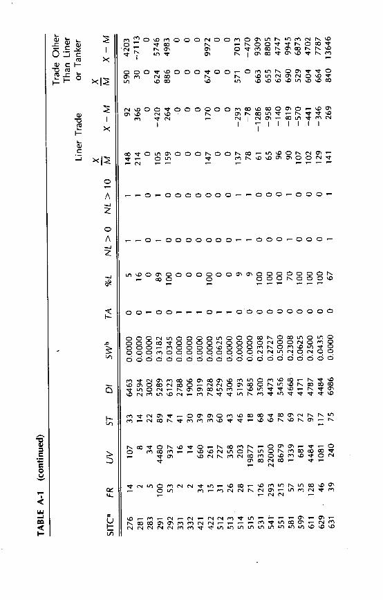
The average values of each variable in the Census data are shown in TableA1 for every SITC group containing at least ten observations. The values forthese variables are not necessarily characteristic of the whole group,particularly in groups with small numbers of observations, since they wereassigned on the basis of the characteristics of the particular observationsthat appeared in the sample.

TA

BLE

A-i

Ave

rage

Val

ues

of V

aria

bles

in C

ensu

s D

ata

..

Tra

de O

ther

Tha

n Li

ner

Line

rT

rade

or T

anke

r

FR

UV

ST

DI

SW

bT

A%

L

xN

L>

0N

L> 1

0M

X —

Mx M

X —

M

11

87

825

82

6882

0.0000

092

10

126

36

165

325

13

50

1231

60

4496

0.0000

0100

00

65

—618

310

3120

31

69

1025

80

4668

0.0000

060

11

112

47

394

2194

32

51

764

60

6597

0.0000

0100

00

165

307

514

6018

51

24

184

113

3242

0.0000

057

11

208

327

365

—2228

53

34

300

59

7196

0.0667

077

11

136

—33

783

8652

55

40

349

62

4854

0.0000

0100

00

175

166

678

6718

61

8117

43

4112

0.0000

10

00

00

00

71

40

806

65

4221

0.0000

0100

10

150

25

172

—1625

72

35

372

68

3670

0.0000

0100

00

123

45

105

—2175

75

99

1945

79

8020

0.0000

0100

00

111

106

376

125

81

25

140

65

3715

0.0000

038

11

87

—203

136

392

99

50

533

65

4301

0.0000

04

11

73

—781

550

7461

112

64

732

65

4250

0.0213

0100

00

96

—585

560

6447

121

66

1416

100

5160

0.0000

0100

00

102

—155

648

4879

211

62

1482

75

5786

0.0000

0100

00

127

70

515

1889

221

19

196

87

5939

0.0000

.0

19

11

120

357

1038

19074

231

51

404

63

8466

0.0000

094

10

120

102

551

390

243

30

140

45

4467

0.0000

097

10

122

74

381

3873

262

90

1659

103

6622

0.0172

0100

00

101

—112

228

1210

266

50

613

97

5751

0.0000

0100

00

114

—442

668

9212

TA

BLE

A-i

(con

tinue

d)

Tra

de O

ther

Tha

n Li

ner

Line

rT

rade

or T

anke

r

.x

x

FR

UV

ST

DI

TA

%L

NL

>0

NL>

10

MX

— M

MX

— M

276

14

107

33

6463

0.0000

05

11

148

92

590

4203

281

28

14

2594

0.0000

016

11

214

366

30

—7113

283

534

22

3002

0.0000

10

00

00

0

291

100

4480

89

5289

0.3182

089

11

105

—420

624

5746

292

53

937

74

6123

0.0345

0100

00

159

264

886

4983

331

216

41

2788

0.0000

10

00

00

00

332

214

30

1906

0.0000

10

.0

00

00

0

421

34

660

39

3919

0.0000

10

00

00

00

422

15

261

39

7828

0.0000

0100

00

147

170

674

9972

512

31

727

60

4529

0.0625

10

00

00

0

513

26

358

43

4306

0.0000

10

00

00

00

514

28

203

46

5193

0.0000

09

11

137

—293

571

7013

515

71

19877

18

7685

0.0000

09

11

78

—78

0—470

531

126

8351

68

3500

0.2308

0100

00

61

—1286

663

9309

541

293

22000

64

4473

0.2727

0100

00

65

—958

655

8805

551

215

8679

78

5456

0.5000

0100

00

96

—140

627

4747

581

57

1339

69

4668

0.2308

070

11

90

—819

690

9945

599

3568

172

4171

0.0625

0100

00

107

—570

529

6873

611

128

4484

97

4787

0.2500

0100

00

102

—441

604

4702

7787

629

.46

1081

117

4484

0.0435

0100

00

129

—346

664

631

39

240

75

6986

0.0000

067

11

141

269

840

13646

•63

264

1

651

652

653

656

657

662

664

665

666

673

674

678

682

687

698

714

715

719

723

724

729

732

821

831

841

851

861

862

86 17

118 81 87 136

148

27 3317

3 92 17 24 22 5210

217

611

013

914

418

824

313

011

528

825

419

631

911

7

ii63

510.

0000

5571

230.

0769

2443

880.

0000

997

650.

0000

6549

790.

5000

027

045

010

00

100

085

010

00

100

O10

00

100

010

00

100

037

010

00

100

010

00

100

010

00

100

1 1 0 0 1

0 0 0 0 0

—10

22—

631

—71

220

4

—30

9—

404

—67

1

—29

6—

253

—15

4—

415

—12

08

766

1204

378

912

147

230

1751

759

8044

671

9803

656

9142

594

7628

569

8448

913

1472

793

816

127

822

1292

867

194

4258

567

4990

214

768

858

1284

476

684

8181

812

629

682

9676

680

8454

850.

1429

176

9247

440.

0000

2361

126

5279

0.05

0015

7310

369

560.

1034

1528

8984

860.

1566

2752

108

6947

0.40

0012

1715

082

380.

0500

215

4263

560.

0000

239

6546

090.

0545

1551

7345

420.

3636

788

6954

000.

1781

9314

6213

0.00

0019

173

010

00

070

1

010

00

010

00

061

1

010

00

010

00

010

00

010

00

010

00

010

00

038

1

274

1030

3589

3943

735

9917

371

4500

628

7883

911

9127

1109

8024

728

1042

911

2911

374

788

1193

468

110

082

679

8619

835

1319

061

287

78

—28

8—

577

—56

1

—17

738

3—

459

220

55—

460

—56

4—

9758

6 4

410

—59

5—

121

—64

4

091

167

080

013

41

188

085

015

70

123

010

2

090

013

01

236

1,15

31

187

059

099

1-

94

066

084

065

014

40

101

010

41

113

083 92 98

109 94 63

5694

121

3664

0.00

0016

8579

4790

0.00

0042

3155

4349

0.30

7715

7856

5188

0.12

5057

3419

863

870.

1600

7842

117

4833

0.18

1815

1918

547

510.

0094

1227

120

4069

0.30

4328

5217

769

730.

4118

4850

202

7766

0.29

8829

3020

551

730.

1600

3011

8363

400.

4194

4231

8038

180.

0909

0 .0 0 0 0 0 1 0 0 0 0 0 0

TA

BLE

A-i

(con

clud

ed)

Tra

de O

ther

Tha

n Li

ner

Line

rT

rade

or T

anke

r

.x

xF

RU

VS

TD

IS

Wb

TA

%L

NL

> 0

NL>

10M

X —

MM

X —

M

891

273

3744

141

6145

01905

010

00

010

9—

3884

912

803

893

116

1209

141

7714

0.00

000

100

00

112

—15

288

814

371

894

270

3026

206

6072

0.27

780

100

00

91—

271

805

1211

989

920

122

2019

170

280.

3947

010

00

012

4—

4283

312

534

SIT

C g

roup

s w

ith te

n or

mor

e ob

serv

atio

ns.

bFig

ure

belo

w m

ultip

lied

by 1

00 is

per

cent

age

of o

bser

vatio

ns o

r gr

oups

with

indi

cate

d ch

arac

teris

tic.

FR

= T

rans

port

cha

rge,

in $

per

tort

.U

V =

Uni

t val

ue, i

n $

per

ton.

ST

= S

tow

age

fact

or, i

n cu

bic

feet

per

ton.

= D

ista

nce,

in n

autic

al m

iles.

SW

= S

mal

l wei

ght d

umm

y fo

r sh

ipm

ents

of l

ess

than

one

ton.

TA

= D

umm

y va

riabl

e fo

r co

mm

odity

gro

up s

omet

imes

impo

rted

into

the

U.S

. by

tank

er.

% L

= P

erce

ntag

e lin

er. F

or p

rodu

cts

neve

r im

port

ed b

y ta

nker

, lin

er im

port

s as

per

cent

age

of s

um o

f lin

er a

nd n

on-li

ner

impo

rts.

NL>

0 =

Non

-line

r gr

eate

r th

an 0

. For

pro

duct

s ne

ver

impo

rted

by

tank

er, d

umm

y va

riabl

e fo

r so

me

non-

liner

impo

rts.

NL>

10

= N

on-li

ner

impo

rts

grea

ter

than

10

per

cent

. For

pro

duct

s ne

ver

impo

rted

by

tank

er, d

umm

y va

riabl

e fo

r no

n-lin

er im

port

s m

ore

than

10

per

cent

of s

um o

f lin

er a

ndno

n-lin

er im

port

s.

= R

atio

of e

xpor

t to

impo

rt to

nnag

e: a

vera

ge fo

r tr

ade

rout

es in

com

mod

ity g

roup

, in

perc

enta

ge.

X —

M =

Diff

eren

ce b

etw

een

expo

rt a

nd im

port

tonn

age:

ave

rage

for

trad

e ro

utes

in c

omm

odity

gro

up, i

n th

ousa

nds

of lo

ng to

ns.

TABLE A-2 Estimating Equations for Transport Charges:.Alternative Equations for Use when Some Var-iables Are Missing

Equation Intercept UV ST DI SW TA R2

(1) —3.53 .52 .35 .30 .30 —.51 .81

(11) —4.42 .56 .38 .35 .25 .80(12) —3.54 .54 .35 .29 —.49 .81

(13) —1.08 .54 .35 .25 —.62 .80(14) —2.50 .59 .31 .28 —.59 .79(15) —4.40 .58 .37 .34 .80(16) —1.66 .60 .39 .18 .79(17) —3.46 .65 .37 .23 .78(18) —1.16 .56 .35 —.60 .80(19) —2.52 .61 .30 —.57 .79(20) —0.02 .61 .23 —.70 .78

(21) —1.71 .61 .38 .78(22) —3.44 .66 .36 .78

(23) —0.57 .68 .15 .76(24) —0.10 .63' —.68 .78(25) —0.62 .69 .76

All variables except SW and TA are in logs.For definitions of variables see Table

TA

BLE

A-3

Tes

ts fo

r N

on-L

inea

rity

in B

asic

Est

imat

ing

Equ

atio

n

Equ

a-to

nIn

ter-

cept

LIV

ST

DI

SW

TA

(LU

)(U

V)

(LS

)(S

T)

(LD

)(D

I)(L

F)(

UV

)(L

F)(

ST

)(L

F)(

D!)

R2

(1)

—3.

53.5

2(5

7.35

).3

5(1

8.18

).3

0(1

3.51

).3

0(6

.22)

—.5

1

(12.

25)

.81

(26)

—3.

57.5

5(3

9.52

).3

6(1

8.41

).2

9(1

2.64

).3

0(6

.35)

—.4

9(1

1.70

)—

.02

(2.8

8).8

1

(27)

—3.

38.5

2(5

7.24

).3

0(1

1.02

).3

0(1

3.57

).2

9(6

.14)

— .5

0

(11.

95)

.02

(2.4

4).8

1

(28)

—4.

39.5

2

(55.

88)

.35

(18.

37)

.41

(10.

56)

.29

(6.1

4)—

.50

(11.

95)

— .0

2

(3.4

9).8

1

(29)

—2.

11.4

3(3

1.19

).1

6(5

.95)

.26

(11.

35)

.23

(5.0

6)—

.53

(13.

43)

—.0

05(0

.24)

.17

(4.7

6).0

1

(0.4

3).8

4

FR

(de

pend

ent v

aria

ble)

= T

rans

port

cha

rge,

in $

per

ton.

UV

Uni

t val

ue, i

n $

per

ton.

ST

= S

tow

age,

in c

ubic

feet

per

ton.

DI

= D

ista

nce,

in n

autic

al m

iles.

SW

Sm

all w

eigh

t dum

my,

for

ship

men

ts o

f les

s th

an o

ne to

n.T

AD

umm

y va

riabl

e fo

r co

mm

odity

gro

up s

omet

imes

impo

rted

into

the

U.S

. by

tank

er.

LULo

w u

nit v

alue

(be

low

the

med

ian)

.LS

= L

ow s

tow

age

fact

or (

belo

w th

e m

edia

n).

LD =

Low

dis

tanc

e (b

elow

the

med

ian)

.LF

= L

ow tr

ansp

ort c

ost )

belo

w th

e m

edia

n).


NOTES AND REFERENCES TO TEXT

1. This analysis of ocean transport charges is a by-product of a study of interrelationsbetween international investment and trade, financed partly from grants to the NationalBureau by the National Science Foundation and the Ford Foundation. Benjamin Chinitz,J. Royce Ginn, Hal B. Lary, Donald S. Shoup, Raymond J. Struyk, and a refereee assistedus with valuable suggestions on both content and presentation, as did Frank Boddy,Emilio C. Collado, Douglass North, Willard Thorp, and Donald Woodward who readthe manuscript as members of the Bureau's Board of Directors. We are indebted toSusan Tebbetts and Marianne Rey for research assistance and programming and to theU.S. Bureau of the Census for some of the data on transport cost. For a description of thestudy see Robert E. Lipsey and Merle Yahr Weiss, "The Relation of U.S. ManufacturingAbroad to U.S. Exports—A Framework for Analysis," 1969 Business and EconomicStatistics Section Proceedings of the American Statistical Association.

2. The most extensive sets of data available are conference rates published in variouscongressional hearings, particularly those of the Joint Economic Committee on Dis-criminatory Ocean Freight Rates and the Balance of Payments. See, for example, 88thCongress, 1st and 2nd Sessions, Parts 1 through 5, June 20 and 21, 1963, October 9 and10, 1963, November 19 and 20, 1963, and March 25 and 26, 1964; and 89th Congress,1st Session, Parts 1, 2, and 3, April 7 and 8, 1965, May 27, 1965, and June 30, 1965. Itis uncertain, however, how closely these match the rates actually paid. Furthermore,they cover only certain trade routes and certain commodities. The commodity descrip-tions usually do not match those of trade data, being sometimes too specific andsometimes too broad. There are also many rates not given in terms of tonnage or valueand not easily translated into those terms. The information is in such cases almostimpossible to relate to trade data without a separate study of each commodity.

3. Jan Tinbergen, Shaping the World Economy (New York: Twentieth Century Fund, 1962),Appendix VI, p. 263.

4. Hans Linnernan, An Econometric Study of Trade Flows (Amsterdam: North-Holland,1966).

5. Grant B. Taplin, "Models of World Trade," International Monetary Fund Staff Papers,November 1967; Edward E. Learner and Robert M. Stern, Quantitative InternationalEconomics (Boston: Allyn and Bacon, 1970), Chapter 6.

6. W. Beckerman, "Distance and the Pattern of Intra-European Trade," Review ofEconomics and Statistics, February 1956, pp. 31—40.

7. For a discussion of the determinants of cost differences among shipping routes seeWalter Oi, "The Cost of Ocean Shipping" in The Economic Value of the United StatesMerchant Marine (Evanston, Illinois: The Transportation Center, 1961).

8. Maritime Freight Rates in the Foreign Trade of Latin America, United Nations, EconomicCommission for Latin America, Joint Transport Programme, November 1970.

9. One of the main intended uses of the equation is for estimating transport charges ifspecific data are not available. Since not all the variables in our equation are alwaysobtainable, we have listed, in Table A2 of the appendix, several variants of the equationthat omit one or more of these variables.

10. For example, A.L. Ginsburg, American and British Regional Export Determinants (Am-sterdam: North-Holland, 1969).

Ii. Irving B. Kravis and Robert E. Lipsey, Price Competitiveness in World Trade (New York:NBER, 1971).

12. We also re-ran our bidding equation for the subset of our observations that matched theindependently collected unit values (Equation 6 in Table 3). The omission of shipmentsfor which we could not collect independent unit values did not affect the Censusequations significantly and we therefore have omitted these calculations.


1 3. See, for example, Herman F. Karreman, Methods for improving World TransportationAccounts, Applied to 1950—1953 (New York: NBER, Technical Paper 15, 1961); andCarmellah Moneta, "The Estimation of Transport Costs in International Trade Accounts,"Journal of Political Economy, February 1959, pp. 41—58.

14. Benjamin Chinitz, "Rate Discrimination in Ocean Transportation," (unpublished Ph.D.dissertation, Harvard University), April 1956.

1 5. Maritime Freight Rates in the Foreign Trade of Latin America, United Nations, EconomicCommission for Latin America, Joint Transport Programme, November 1970.

16. See, for example, the Joint Economic Committee's hearings on Discriminatory OceanFreight Rates and the Balance of Payments.

NOTES AND REFERENCES TO APPENDIX

1. "C.l.F. Calculations Add 9 Percent to Import Figures, Special Study Shows," CensusBureau release, December 20, 1966; and Kravis and Lipsey, Price Competitiveness inWorld Trade (see Chapter 4 for a description of data sources).

2. The ratio was virtually identical to the average of 1968—70. The results of these surveyswere reported in Highlights of U.S. Export and import Trade (FT 990), U.S. Bureau of theCensus, March 1969, July 1970, and April 1972.

3. The equation for weight was:

log weight (pounds) = 3.2802 + .7755 capacity (KVA)

(10.67) (26.31)

and the equation for stowage was:

log stowage (cubic feet per ton) = 42.06 — .03 capacity (KVAI1 ,000)(4.08)

Numbers in parentheses are t-values of regression coefficients.4. Railway Age, January 18, 1960; January 15, 1962; January 20, 1964; Simmons-

Boardman Publishing Corp.5. The equation was:

log weight (pounds) = 7.79 + .65 log HP + .09CC — .246

(54.07) (29.76) (3.20) (4.80)

— .38 Gen'I Purpose — .27 Rd. Switch(11.82) (8.27)— .27 Freight — .45 Misc. Purpose(5.73) (10.52)

in which HP is horsepower, CC and B are wheel arrangements, and General Purpose,Road Switching, Freight, and Miscellaneous describe the type of service for which thelocomotives were built. Numbers in parentheses are t-values of regression coefficients.

6. Alcoa Product Data: Aluminum Electrical Conductors, Stranded-Bare, December 1,1966 (Pittsburgh: Aluminum Co. of America).

7. For empirical evidence for this statement see Moneta, "The Estimation of TransportCosts . .

8. Data were taken from Commodity Trade: Exports, Series C, January—December 1 964,OECD.

9. U.S. Bureau of the Census, U.S. General Imports-Geographic Area, Country, ScheduleA: Commodity Groupings, and Method of Transportation, Report FT 155, Annual 1967,Washington, 1968.


10. The stowage factors were taken from R.E. Thomas and 0.0. Thomas, Stowage: TheProperties and Stowage of Cargoes (Glasgow: Brown, Son & Ferguson, Ltd., 1968); fromThe Stowage Red Book (New York: Traffic Publishing Co., 1944); and from G.P. Lewis,Handy Guide to Stowage (London and St. Ives Hunts: Imroy, Laurie, Node & Wilson,Ltd., 1962).

11. See the Marine Distance and Speed Table (New York: Edward W. Sweetman Co., 1965),and Table of Distances Between Ports (U.S. Navy Department, Hydrographic Office,1943).

12. Essential United States Foreign Trade Routes, Maritime Administration, U.S. Departmentof Commerce, Washington, 1969.

Documents

The Structure of Ocean Transport Charges · Several empirical models of international trade flows, ... neighborhood of .50. ... chiefly value at the point of shipment,