Noname manuscript No.(will be inserted by the editor)

The Structure and Dynamics of the Corona – HeliosphereConnection

Spiro K. Antiochos · Jon A. Linker · RobertoLionello · Zoran Miki c · Viacheslav Titov ·Thomas H. Zurbuchen

Received: date / Accepted: date

Abstract Determining the source at the Sun of the slow solar wind is oneof the major un-solved problems in solar and heliospheric physics. First, we review the existing theories forthe slow wind and argue that they have difficulty accounting for both the observed composi-tion of the wind and its large angular extent. A new theory in which the slow wind originatesfrom the continuous opening and closing of narrow open field corridors, the S-Web model,is described. Support for the S-Web model is derived from MHDsolutions for the quasi-steady corona and wind during the time of the August 1, 2008 eclipse. Additionally, weperform fully dynamic numerical simulations of the corona and heliosphere in order to testthe S-Web model as well as the interchange model proposed by Fisk and co-workers. Wediscuss the implications of our simulations for the competing theories and for understandingthe corona – heliosphere connection, in general.

Keywords Sun: corona· Sun: solar wind

1 Introduction

Since the pioneering theoretical work of Parker (1958, 1963) and the discovery observa-tions of Neugebauer & Snyder (1962) it has been known that theSun’s atmosphere streamscontinuously outward in the form of a supersonic wind. This wind carries both plasma andmagnetic field to the boundary of the solar system, the heliopause. At a basic level, the ori-gins of the wind are straightforward. As argued by Parker, the difference in gas pressurebetween the Sun’s hot, 1 MK, corona and the tenuous interstellar gas causes the coronal

S. K. AntiochosNASA Goddard Space Flight Center, Code 674, Greenbelt, MD 20771, USATel.: +1-301-286-8849Fax: +1-301-286-1648E-mail: spiro.antiochos@nasa.gov

J. A. Linker, R. Lionello, Z. Mikic, V. TitovPredictive Science, Inc., 9990 Mesa Rim Rd., Ste. 170, San Diego, CA 92121, USA

T. H. ZurbuchenDepartment of Atmospheric, Oceanic and Space Sciences, College of Engineering, University of Michigan,2455 Hayward St, Ann Arbor, Michigan 48109

https://ntrs.nasa.gov/search.jsp?R=20110008367 2019-04-05T19:26:46+00:00Z

2

gas to expand outward. If the heating to the corona is constant, then the wind can adopt thesteady state described by Parker’s original theory.

Of course, on the real Sun there are many added complicationsto Parker’s simple steady-state model. The first and foremost is the presence of the solar magnetic field. This naturallydivides the corona into two physically distinct regions. Inthose regions where the field isstrong, such as deep inside an active region, the field prevents the plasma from expanding;thereby resulting in an approximately static coronal plasma. These regions are referred to as“closed”, because all field lines are connected to the photosphere at two ends. The closedflux is truly coronal in that it does not connect to the heliosphere, but appears instead asthe well-known X-ray coronal loops (e.g., Orrall 1981). On the other hand, in those regionswhere the field is weak and the gas dominates, the gas pressuredrags the field lines outwardindefinitely. These regions are referred to as “open” in thatthe field lines have only one endconnected to the photosphere. The outward mass and energy flow in open regions resultsin a decreased density there, so that they appear as “coronalholes” in X-ray images (e.g.,Zirker 1977). Note that for a true steady state, the solar wind and the heliospheric magneticflux originate solely from photospheric/coronal open-fieldregions.

In addition to introducing the complication of topology to the corona and heliosphere,the magnetic field also forces them to be fully time dependent. Since the distribution of fluxat the photosphere is constantly changing due to flux emergence/cancellation and a broadrange of photospheric flows, the distribution of open and closed flux must change, as well,implying that the solar wind is inherently dynamic. Consequently Parker’s theory can be, atbest, a quasi-steady approximation to the actual state of the corona and wind.

The dynamics introduced to the solar wind by the photospheric field evolution naturallybreaks up into different regimes determined by the time required for establishing a steadywind. This is of order a few travel times to the Alfven radius,∼ 20 R⊙, which implies a timescale of ten hours or so. Since the photospheric evolution has a more-or-less constant speedof 1 km/s or less, the time scale translates directly to a sizescale for the photospheric dy-namics. Large-scale phenomena, such as the differential rotation or the emergence/dispersalof large active regions occurs over days, and so could be incorporated within the quasi-steady approximation. Small-scale phenomena, however, such as the magnetic carpet (Har-vey 1985; Schrijver et al. 1997) or granular flows have time scales typically less than a fewhours and, hence, can be considered as a constant source of fluctuations or noise to the quasi-steady state. Intermediate between these spatial scales isthe typical size of supergranules,whose lifetimes are of order that required to establish a steady state. It is likely that theireffect on the wind can be determined properly only by explicit time-dependent calculations.

In the heliosphere, the photospheric dynamics appear to structure the solar wind via themediation of the magnetic field into two distinct forms, the so-called fast and slow winds.The fast wind has speeds generally in excess of 500 km/s, but that is not its distinguishingfeature. This wind has 3 defining features: (a) its temporal variations, (b) spatial location,and (c) plasma composition.

(a) As shown clearly by the Ulysses measurements, the high-latitude fast wind exhibitsnear constant speed (McComas et al. 2008) and composition (Geiss et al. 1995; von Steigeret al. 1995; Zurbuchen 2007). Its observed variability consists primarily of Alfvenic fluctu-ations that may be due entirely to the expected dynamics induced by the small-scale photo-spheric evolution described above.

(b) The fast wind originates inside non-transient (lifetime> 1 day) coronal holes, wherethe field has been open for a sufficient duration to establish asteady state.

(c) The fast wind has elemental abundances close to that of the photosphere (von Steigeret al. 1997, 2001; Zurbuchen et al. 1999, 2002). It does not exhibit the FIP bias of the closed-

3

field corona (Meyer 1985; Feldman & Widing 2003). Furthermore, its ionic composition issteady and implies a freeze-in temperature near the Sun around or below 1 MK (Zurbuchen2007).

From these properties, we conclude that the fast wind is the true quasi-steady wind of theoriginal Parker theory. The slow wind, on the other hand, is completely different. Its speedsare generally< 500 km/s, but again, this is not the distinguishing feature.The 3 definingfeatures of this wind are markedly different than those above:

(a) The slow wind is intrinsically variable, both in speed and, especially, composition(Zurbuchen & von Steiger 2006; Zurbuchen 2007). The velocity structure consists of peri-ods of fast flows intermingled with slow. This variation is not simply Alfvenic fluctuationssuperimposed on a quasi-steady state. Certainly the large compositional variability, both inelemental and ion-temperatures, cannot be due to turbulence in the flow, but reflects insteadan intrinsic difference in the origins of the fast and slow wind.

(b) The slow wind is associated with the heliospheric current sheet (HCS), which isalways embedded in slow wind, not fast (Burlaga et al. 2002).On the other hand, the slowwind is observed to extend in the heliosphere to angles far from the HCS, up to 30◦ or so.

(c) The slow wind has elemental composition (FIP bias) closeto that of the closed fieldcorona. Its ionic composition implies a freeze-in temperature near the Sun (∼ 1.5 MK),considerably higher than that of the fast (Zurbuchen et al. 2002). Furthermore, the elementaland ionic compositions are highly variable, unlike the steady composition of the fast. A keypoint is that, as defined by the composition, the boundary between the fast and slow windsis narrow, of order a few degrees or so (Zurbuchen et al. 1999), which is small compared tothe angular extent of either the slow or fast winds.

The results that the slow wind is associated with the HCS, which maps down to theY-line at the top of the helmet streamer belt, and that the slow wind has the compositionof the closed corona suggest that it somehow originates fromnear or inside the closed fieldregion. The most obvious scenario is that it is due to the interaction between closed andopen fields, which releases closed field plasma onto open fieldlines. This would naturallyaccount for both its observed variability and composition.The problem, however, is that theslow wind does sometimes extend far from the HCS in latitude,which implies that its sourceat the Sun is inside the open field region, far from the open-closed field boundary. But inthat case, it is difficult to understand why its composition should resemble that of closedfield plasma. These apparently conflicting observations have long made the identification ofthe solar sources of the slow wind one of the major unsolved problems in Heliophysics. Wedescribe below the basic theories that have been proposed for the slow wind sources, presentsome numerical tests of one of these theories (Linker et al. 2011), and describe a new theoryfor the slow wind, the S-Web model (Antiochos et al. 2011).

2 Theories for the Sources of the Slow Wind

There are essentially three different possibilities for the slow wind source: It originates inthe open field region, just like the fast; it somehow originates from inside the closed fieldregion; or it originates from the streamer tops, at the boundary between open and closed. Wediscuss each of them, in turn, below, but focus on the streamer top model and propose anextension of this theory, the S-Web model, that can reconcile the theory with observations.

4

2.1 The Expansion Factor Model

Perhaps, the simplest theory for the slow wind is that it originates from open field near theboundary between open and closed (Suess 1979; Kovalenko 1981; Withbroe 1988; Wang& Sheeley 1990; Cranmer & van Ballegooijen 2005; Cranmer et al. 2007). This scenario ishighly appealing in that it implies a unified theory for the origins of the fast and slow winds.Both are due to a single mechanism: photospherically-driven MHD waves deposit heat andmomentum to coronal plasma, resulting in a Parker-like solar wind outflow. The key ideaunderlying the model is that the speed of the wind is sensitive to the exact locations of theheat and momentum deposition in an open flux tube; in particular, heating low down belowthe critical point leads to a hotter, slower wind (Holzer & Leer 1980). The observed dif-ferences between the fast and slow winds, therefore, may arise solely from the geometricaldifference between flux tubes near the coronal hole boundaryversus those deep in the inte-rior. Flux tubes near the boundary expand super-radially from the photosphere to a height oforder a few solar radii; whereas those near the interior expand radially or even sub-radially.Even if the photospheric flux of waves into all flux tubes in a coronal hole is the same, theevolution of the waves in the corona, (the resulting turbulence and dissipation), will dependon the geometry of the flux tube. Cranmer and co-workers have argued that all the distin-guishing features of the slow wind, including the variability and elemental composition canbe explained by the effect of the flux tube geometry, the so-called expansion factor, on thewave evolution.

The challenge for the expansion factor theory is that the speed of the solar wind issometimes observed to be slow, but the wind still has the variability, composition, and otherfeatures indicative of the fast wind. Zhao et al. (2009) haveshown that the wind from smalllow-latitude coronal holes with large expansion factors is, indeed, slow,∼ 500 km/s; butthis wind still has all the temporal and compositional characteristics of the fast wind. Theseobservations are in direct conflict with any model proposingthat the differences betweenthe fast and slow wind result solely from differences in flux tube geometry. The Zhao et al.(2009) results demonstrate that a large expansion factor inan open flux tube does slow downthe wind, as predicted, but it does not lead to the variability and composition observed in theslow wind. We conclude, therefore, that the expansion factor model, as presently described,is not consistent with the observations.

2.2 The Interchange Model

Another theory for the slow wind is the interchange model proposed by Fisk and co-workers(Fisk et al. 1998; Fisk 2003; Fisk & Zhao 2009), which in many ways is the diametricopposite of the expansion factor model. In the interchange model the slow wind is postulatedto originate from the closed field region via continuous interchange reconnection betweenopen field lines and the closed flux. Consequently, this modelis intrinsically dynamic; thereis no steady state solar wind, at least, for the slow component. Note also that there is no trulyclosed field region, because the open flux is postulated to diffuse throughout the apparentlyclosed field regions outside coronal holes. The key idea underlying the model is that theevolution of the coronal open flux is dominated by the continuous small-scale dynamics ofthe photosphere, such as emergence/cancellation of magnetic carpet bipoles, which drivereconnection between open flux and closed. In addition to being fundamentally dynamicrather than steady, the interchange model also proposes a completely different magnetictopology than the expansion factor model. In the latter, thetopology is smooth with well

5

separated open and closed field regions, but in the former thetopology is essentially chaoticwith open and closed flux mixing indiscriminately.

In terms of accounting for slow wind observations, the advantages of the interchangemodel are obvious. It naturally produces a continuously variable wind with closed field com-position and located around the HCS, but with large extent. The primary challenge for themodel is to verify that interchange reconnection induced byphotospheric dynamics does,indeed, produce the required diffusion of open flux into closed field regions. Argumentshave been presented by Antiochos et al. (2007) that basic Lorentz force balance consid-erations prohibit the mixing of open flux with closed. In fact, Antiochos et al argued thatthe open-closed topology remains smooth even during interchange reconnection and haveproposed theorems that severely constrain the possible topologies of the Sun’s open fieldregions. These authors, however, did not perform an actual dynamic calculation of the ef-fect of interchange reconnection with magnetic carpet bipoles on open flux evolution. Wepresent just such a calculation in the following section. Aswill be evident below, the resultsof this calculation donot support the underlying assumptions of the interchange model. Ourresults, however, do support key aspects of the interchangemodel in that dynamics and astatistical approach are likely to be essential for modeling the slow wind.

2.3 The Streamer-Top Model

The third theory for the source of the slow wind, the streamer-top model, is in some ways,a compromise between the expansion factor and interchange models. The basic idea is thatthe boundary between the open and closed flux, the edge of a streamer, is either unstable(Suess et al. 1996; Endeve et al. 2004; Rappazzo et al. 2005) or sensitive to perturbationsand, consequently, undergoes continuous dynamics (Mikicet al. 1999). In response to pho-tospheric changes or other disturbances, closed flux near the streamer boundary expandsoutward and becomes open and open flux reconnects at the HCS tobecome closed. Further-more, interchange reconnection can occur at the streamer tops in response to photosphericchanges (e.g., Wang et al. 2000). These processes will naturally release closed field plasmainto the solar wind and produce a variable wind with the observed composition. Note thatin this model the source of the slow wind is the boundary region between open and closedflux, similar to the expansion factor model, but the boundaryin this case is fully dynamicand involves the continual interchange of open and closed flux. In this respect the model issimilar to the interchange model, but the open-closed interchange in the streamer-top modeloccurs only near the streamer boundary. There is no diffusion of open flux deep inside theclosed-field streamer.

There are a number of observations that provide compelling support for the streamer-top model. Movies of coronal evolution often show the upwardexpansion and eventualopening of closed loops (Hundhausen et al. 1984; Howard et al. 1985; Sheeley & Wang2002). Conversely, coronagraph observations frequently show blobs streaming outward nearthe current sheet and reconnection events at the HCS (Sheeley 1997), as required for thestreamer-top model. In the heliosphere the HCS is observed to be clearly dynamic withno evidence for a simple field reversal as would be the case fora quasi-steady wind. Weconclude, therefore, that the boundary between the open andclosed flux in the corona is,indeed, highly dynamic and, therefore, will be the source ofa variable slow wind.

The problem, however, is that these dynamics are expected tobe confined to a relativelynarrow region about the streamer boundary, or equivalently, about the HCS. Assuming thatthe open-closed boundary is “blurred” by the photospheric dynamics over a scale of order a

6

supergranule radius,∼ 30,000 km, we derive an angular extent for this dynamic wind of nomore than 5◦. In fact, this width is what is observed for the streamer stalks emanating fromthe tops of streamers and for the so-called plasma sheet in the heliosphere (Winterhalter etal. 1994; Wang et al. 2007). But this angular width is far too small to explain the slow windwhich has been observed to extend out to 30◦ from the HCS. Explaining the large angularextent of the slow wind is the fundamental challenge for the streamer-top model. Sincethe boundary between open and closed flux maps directly to theHCS, it seems unlikelythat blurring this boundary by a small distance on the Sun would ever produce effects inthe heliosphere far from the HCS. We describe below our theory, the S-Web model, thataccomplishes exactly this unlikely result.

3 The S-Web Model

In previous work (Antiochos et al. 2007) we proposed theuniqueness conjecture, whichstates that any unipolar region on the photosphere can contain at most one coronal hole.However, low-latitude coronal holes that appear to be disconnected from their correspondingpolar hole are frequently observed on the Sun (e.g., Kahler &Hudson 2002). We argued thatin these cases, the low-latitude satellite hole is actuallyconnected to the main polar hole bya narrow open field corridor whose width is below the spatial resolution of the observations.Note also that if the corridor is sufficiently narrow, it willbe obscured by neighboring closedfield regions with much higher brightness.

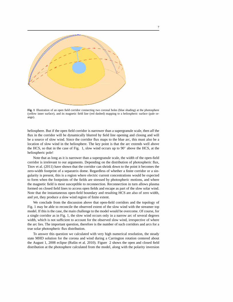
Let us consider how such a corridor would map into the heliosphere. For illustrativepurposes, Figure 1 shows such a mapping in the extreme case where the polar hole andsatellite holes have near equal flux. The inner hemisphere corresponds to the photosphere,with the dark yellow region representing the closed field andthe light blue representingthe two coronal holes connected by an open-field corridor. The light orange hemispherecorresponds to some surface in the heliosphere where the field is all open, say at 10 R⊙. Onthis surface the radial flux is approximately uniformly distributed, as in the real heliosphere,and there is a single HCS, indicated by the black line runningaround the equator of the 10R⊙ surface. Note that this HCS maps down to the boundary of the single, (topologicallyconnected), open field region on the photosphere. Four field lines with footpoints near the“end points” of the open field corridor are drawn, illustrating this mapping from the HCS tothe open field boundary.

If the holes have roughly equal flux, their flux must divide the10 R⊙ surface into twonear equal halves. In Fig. 1, the satellite hole maps to the near half and the polar to the far.Separating these halves is a thin arc, blue curve on the 10 R⊙ surface, that maps to the openfield corridor. Note that this arc divides the heliospheric surface and, hence, must extend tonear 90◦ from the HCS. If the open-field corridor is very narrow, then the field-line mappingfrom the blue arc down to the solar surface is quasi-singular, so topologically, the arc is aso-called quasi-separatrix layer (Priest & Demoulin 1995; Demoulin et al. 1996; Titov et al.2002). The HCS, on the other hand, is a true separatrix, because the field-line mapping issingular there.

Figure 1 illustrates a steady model, but to obtain the slow wind we need to add thetemporal variability. Assume that due to the random photospheric evolution, the open-closedboundary at the photosphere becomes dynamically blurred bycontinuous field line openingand closing over some finite width, such as a supergranule scale. This narrow boundaryregion is now a source of slow wind. Due to the field line mapping, the HCS also acquiresa finite angular width of order several degrees, and becomes alocation for slow wind in the

7

Fig. 1 Illustration of an open field corridor connecting two coronal holes (blue shading) at the photosphere(yellow inner surface), and its magnetic field line (red dashed) mapping to a heliospheric surface (pale or-ange).

heliosphere. But if the open field corridor is narrower than asupergranule scale, thenall theflux in the corridor will be dynamically blurred by field line opening and closing and willbe a source of slow wind. Since the corridor flux maps to the blue arc, this must also be alocation of slow wind in the heliosphere. The key point is that the arc extends well abovethe HCS, so that in the case of Fig. 1, slow wind occurs up to 90◦ above the HCS, at theheliospheric pole!

Note that as long as it is narrower than a supergranule scale,the width of the open-fieldcorridor is irrelevant to our arguments. Depending on the distribution of photospheric flux,Titov et al. (2011) have shown that the corridor can shrink down to the point it becomes thezero-width footprint of a separatrix dome. Regardless of whether a finite corridor or a sin-gularity is present, this is a region where electric currentconcentrations would be expectedto form when the footpoints of the fields are stressed by photospheric motions, and wherethe magnetic field is most susceptible to reconnection. Reconnection in turn allows plasmaformed on closed field lines to access open fields and escape aspart of the slow solar wind.Note that the instantaneous open-field boundary and resulting HCS are also of zero width,and yet, they produce a slow wind region of finite extent.

We conclude from the discussion above that open-field corridors and the topology ofFig. 1 may be able to reconcile the observed extent of the slowwind with the streamer topmodel. If this is the case, the main challenge to the model would be overcome. Of course, fora single corridor as in Fig. 1, the slow wind occurs only in a narrow arc of several degreeswidth, which is not sufficient to account for the observed slow wind, irrespective of wherethe arc lies. The important question, therefore is the number of such corridors and arcs for atrue solar photospheric flux distribution.

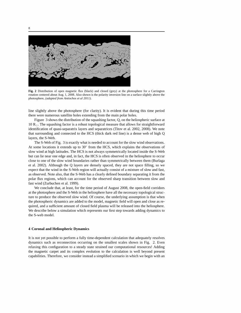
To answer this question we calculated with very high numerical resolution, the steadystate MHD solution for the corona and wind during a Carrington rotation centered aboutthe August 1, 2008 eclipse (Rusin et al. 2010). Figure 2 shows the open and closed fielddistribution at the photosphere calculated from the model,along with the polarity inversion

8

Fig. 2 Distribution of open magnetic flux (black) and closed (grey)at the photosphere for a Carringtonrotation centered about Aug. 1, 2008. Also shown is the polarity inversion line on a surface slightly above thephotosphere,(adapted from Antiochos et al 2011).

line slightly above the photosphere (for clarity). It is evident that during this time periodthere were numerous satellite holes extending from the mainpolar holes.

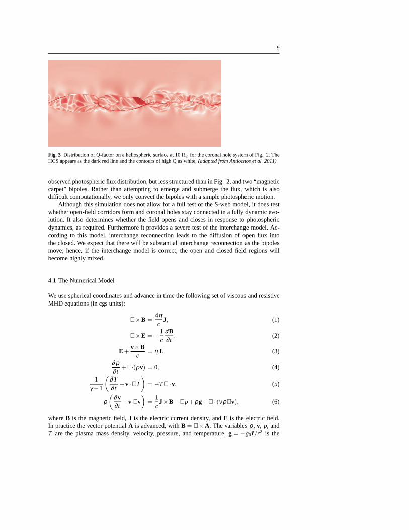
Figure 3 shows the distribution of the squashing factor, Q, on the heliospheric surface at10 R⊙. The squashing factor is a robust topological measure that allows for straightforwardidentification of quasi-separatrix layers and separatrices (Titov et al. 2002, 2008). We notethat surrounding and connected to the HCS (thick dark red line) is a dense web of high Qlayers, the S-Web.

The S-Web of Fig. 3 is exactly what is needed to account for theslow wind observations.At some locations it extends up to 30◦ from the HCS, which explains the observations ofslow wind at high latitudes. The HCS is not always symmetrically located inside the S-Webbut can lie near one edge and, in fact, the HCS is often observed in the heliosphere to occurclose to one of the slow wind boundaries rather than symmetrically between them (Burlagaet al. 2002). Although the Q layers are densely spaced, they are not space filling, so weexpect that the wind in the S-Web region will actually consist of a mixture of slow and fast,as observed. Note also, that the S-Web has a clearly defined boundary separating it from thepolar flux regions, which can account for the observed sharp transition between slow andfast wind (Zurbuchen et al. 1999).

We conclude that, at least, for the time period of August 2008, the open-field corridorsat the photosphere and the S-Web in the heliosphere have all the necessary topological struc-ture to produce the observed slow wind. Of course, the underlying assumption is that whenthe photospheric dynamics are added to the model, magnetic field will open and close as re-quired, and a sufficient amount of closed field plasma will be released into the heliosphere.We describe below a simulation which represents our first step towards adding dynamics tothe S-web model.

4 Coronal and Heliospheric Dynamics

It is not yet possible to perform a fully time-dependent calculation that adequately resolvesdynamics such as reconnection occurring on the smallest scales shown in Fig. 2. Evenrelaxing this configuration to a steady state strained our computational resources! Addingthe magnetic carpet and its complex evolution to the calculation is well beyond presentcapabilities. Therefore, we consider instead a simplified scenario in which we begin with an

9

Fig. 3 Distribution of Q-factor on a heliospheric surface at 10 R⊙ for the coronal hole system of Fig. 2. TheHCS appears as the dark red line and the contours of high Q as white, (adapted from Antiochos et al. 2011)

observed photospheric flux distribution, but less structured than in Fig. 2, and two “magneticcarpet” bipoles. Rather than attempting to emerge and submerge the flux, which is alsodifficult computationally, we only convect the bipoles witha simple photospheric motion.

Although this simulation does not allow for a full test of theS-web model, it does testwhether open-field corridors form and coronal holes stay connected in a fully dynamic evo-lution. It also determines whether the field opens and closesin response to photosphericdynamics, as required. Furthermore it provides a severe test of the interchange model. Ac-cording to this model, interchange reconnection leads to the diffusion of open flux intothe closed. We expect that there will be substantial interchange reconnection as the bipolesmove; hence, if the interchange model is correct, the open and closed field regions willbecome highly mixed.

4.1 The Numerical Model

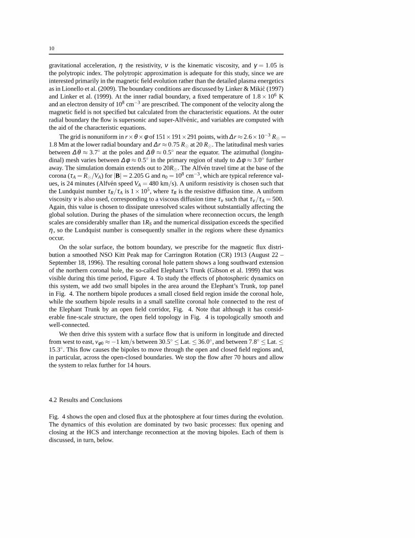
We use spherical coordinates and advance in time the following set of viscous and resistiveMHD equations (in cgs units):

∇×B =4πc

J, (1)

∇×E = −1c

∂B∂ t

, (2)

E+v×B

c= ηJ, (3)

∂ ρ∂ t

+∇·(ρv) = 0, (4)

1γ −1

(

∂ T∂ t

+v ·∇T

)

= −T ∇ ·v, (5)

ρ(

∂v∂ t

+v·∇v)

=1c

J×B−∇p+ρg+∇ · (νρ∇v), (6)

whereB is the magnetic field,J is the electric current density, andE is the electric field.In practice the vector potentialA is advanced, withB = ∇×A. The variablesρ , v, p, andT are the plasma mass density, velocity, pressure, and temperature,g = −g0r/r2 is the

10

gravitational acceleration,η the resistivity,ν is the kinematic viscosity, andγ = 1.05 isthe polytropic index. The polytropic approximation is adequate for this study, since we areinterested primarily in the magnetic field evolution ratherthan the detailed plasma energeticsas in Lionello et al. (2009). The boundary conditions are discussed by Linker & Mikic (1997)and Linker et al. (1999). At the inner radial boundary, a fixedtemperature of 1.8×106 Kand an electron density of 108 cm−3 are prescribed. The component of the velocity along themagnetic field is not specified but calculated from the characteristic equations. At the outerradial boundary the flow is supersonic and super-Alfvenic,and variables are computed withthe aid of the characteristic equations.

The grid is nonuniform inr×θ ×φ of 151×191×291 points, with∆r ≈2.6×10−3 R⊙ =1.8 Mm at the lower radial boundary and∆r ≈ 0.75R⊙ at 20R⊙. The latitudinal mesh variesbetween∆θ ≈ 3.7◦ at the poles and∆θ ≈ 0.5◦ near the equator. The azimuthal (longitu-dinal) mesh varies between∆φ ≈ 0.5◦ in the primary region of study to∆φ ≈ 3.0◦ furtheraway. The simulation domain extends out to 20R⊙. The Alfven travel time at the base of thecorona (τA = R⊙/VA) for |B|= 2.205 G andn0 = 108 cm−3, which are typical reference val-ues, is 24 minutes (Alfven speedVA = 480 km/s). A uniform resistivity is chosen such thatthe Lundquist numberτR/τA is 1×105, whereτR is the resistive diffusion time. A uniformviscosityν is also used, corresponding to a viscous diffusion timeτν such thatτν/τA = 500.Again, this value is chosen to dissipate unresolved scales without substantially affecting theglobal solution. During the phases of the simulation where reconnection occurs, the lengthscales are considerably smaller than 1RS and the numerical dissipation exceeds the specifiedη , so the Lundquist number is consequently smaller in the regions where these dynamicsoccur.

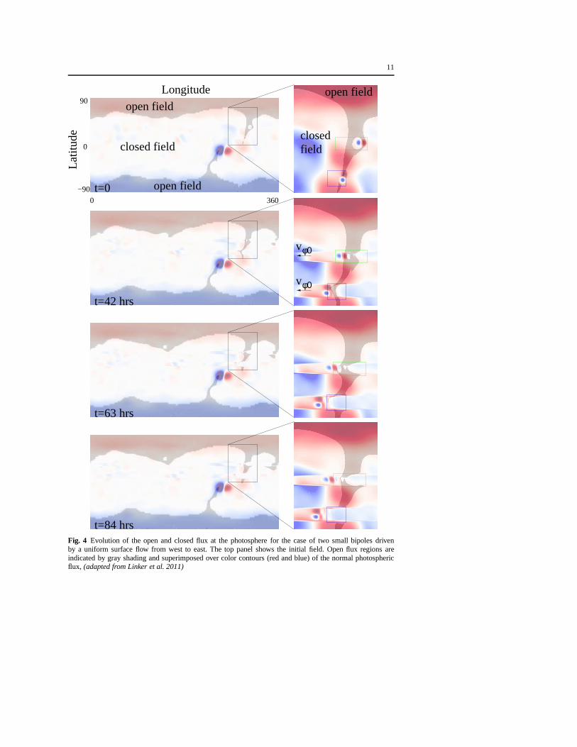
On the solar surface, the bottom boundary, we prescribe for the magnetic flux distri-bution a smoothed NSO Kitt Peak map for Carrington Rotation (CR) 1913 (August 22 –September 18, 1996). The resulting coronal hole pattern shows a long southward extensionof the northern coronal hole, the so-called Elephant’s Trunk (Gibson et al. 1999) that wasvisible during this time period, Figure 4. To study the effects of photospheric dynamics onthis system, we add two small bipoles in the area around the Elephant’s Trunk, top panelin Fig. 4. The northern bipole produces a small closed field region inside the coronal hole,while the southern bipole results in a small satellite coronal hole connected to the rest ofthe Elephant Trunk by an open field corridor, Fig. 4. Note thatalthough it has consid-erable fine-scale structure, the open field topology in Fig. 4is topologically smooth andwell-connected.

We then drive this system with a surface flow that is uniform inlongitude and directedfrom west to east,vφ0 ≈−1 km/s between 30.5◦ ≤ Lat.≤ 36.0◦, and between 7.8◦ ≤ Lat.≤15.3◦. This flow causes the bipoles to move through the open and closed field regions and,in particular, across the open-closed boundaries. We stop the flow after 70 hours and allowthe system to relax further for 14 hours.

4.2 Results and Conclusions

Fig. 4 shows the open and closed flux at the photosphere at fourtimes during the evolution.The dynamics of this evolution are dominated by two basic processes: flux opening andclosing at the HCS and interchange reconnection at the moving bipoles. Each of them isdiscussed, in turn, below.

11

t=0

Latit

ude

Longitude

0

0

−90

360

closed fieldclosedfield

open fieldopen field

open field

90

t=84 hrs

t=63 hrs

t=42 hrs

vφ0

vφ0

Fig. 4 Evolution of the open and closed flux at the photosphere for the case of two small bipoles drivenby a uniform surface flow from west to east. The top panel showsthe initial field. Open flux regions areindicated by gray shading and superimposed over color contours (red and blue) of the normal photosphericflux, (adapted from Linker et al. 2011)

12

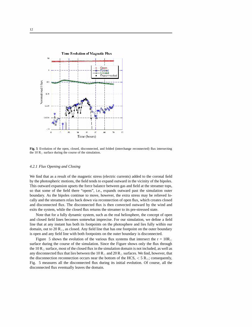
Fig. 5 Evolution of the open, closed, disconnected, and folded (interchange reconnected) flux intersectingthe 10 R⊙ surface during the course of the simulation.

4.2.1 Flux Opening and Closing

We find that as a result of the magnetic stress (electric currents) added to the coronal fieldby the photospheric motions, the field tends to expand outward in the vicinity of the bipoles.This outward expansion upsets the force balance between gasand field at the streamer tops,so that some of the field there “opens”, i.e., expands outwardpast the simulation outerboundary. As the bipoles continue to move, however, the extra stress may be relieved lo-cally and the streamers relax back down via reconnection of open flux, which creates closedand disconnected flux. The disconnected flux is then convected outward by the wind andexits the system, while the closed flux returns the streamer to its pre-stressed state.

Note that for a fully dynamic system, such as the real heliosphere, the concept of openand closed field lines becomes somewhat imprecise. For our simulation, we define a fieldline that at any instant has both its footpoints on the photosphere and lies fully within ourdomain, out to 20 R⊙, as closed. Any field line that has one footpoint on the outer boundaryis open and any field line with both footpoints on the outer boundary is disconnected.

Figure 5 shows the evolution of the various flux systems that intersect the r = 10R⊙surface during the course of the simulation. Since the Figure shows only the flux throughthe 10 R⊙ surface, most of the closed flux in the simulation domain is not included, as well asany disconnected flux that lies between the 10 R⊙ and 20 R⊙ surfaces. We find, however, thatthe disconnection reconnection occurs near the bottom of the HCS,< 5 R⊙; consequently,Fig. 5 measures all the disconnected flux during its initial evolution. Of course, all thedisconnected flux eventually leaves the domain.

13

Fig. 5 verifies the basic premise of the streamer-top and S-web models. In response tophotospheric stressing, magnetic flux opens and closes at the HCS. Although we do not trackit explicitly, there is clearly release of closed field plasma into the wind. For the localizedboundary motions of our simulations, the flux opening/closing is small; we note from Fig. 5that the open flux increases only slightly during the simulation and the disconnected flux isalways 3 orders of magnitude or more smaller than the open. Ifwe were to impose randommotions throughout the photosphere, as in the Sun, the flux opening and closing wouldbe much more pronounced. The key point, however, is that there is definitely opening andclosing at the HCS, in agreement with the S-web model, but in direct conflict with the basicpremise of the interchange model (Fisk et al. 1998; Fisk 2003).

An important conclusion from our results is that closed and disconnected flux should becontinuously present in the heliosphere near the HCS. In fact the HCS is well known to bea region of continuous dynamics; for example, the field is rarely observed to vanish there aswould be expected for a true steady state. On the other hand, closed and disconnected fieldlines should exhibit distinct electron heat-flux signatures in the heliosphere (e.g., Gosling1990; McComas et al. 1991). These signatures are frequentlyobserved in ICMEs, whichclearly do involve substantial flux opening and closing, butthey are rarely seen outsideCMEs (Gosling 1990; Pagel et al. 2005), suggesting that the slow wind flux is not openingand closing. Reconciling this apparent disagreement with the heliospheric electron heat fluxmeasurements, which may require re-interpretation of the electron data (Crooker & Pagel2008), remains one of the major challenges for all solar windmodels.

4.2.2 Interchange Reconnection

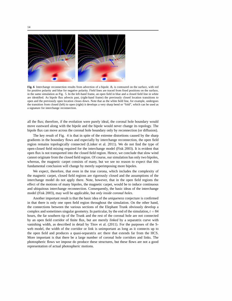
The other major form of dynamics found in our simulation is that of interchange reconnec-tion between the flux of the small bipoles and the surroundingfield. The magnetic topologyof each bipole is simply that of the well-known embedded bipole with its fan separatrixsurface, pair of spine lines, and coronal null point (e.g., Antiochos 1990; Antiochos et al.2007). The photospheric motions stress the separatrix and null, creating current sheets there,which leads to reconnection between the closed field associated with the parasitic polarityof the bipole and the external flux (see Figure 6). If this flux is open, then the reconnectionis of the interchange type; if it is closed, the reconnectionmerely exchanges closed flux(Edmondson et al. 2009; Linker et al. 2011).

Since interchange reconnection, like all reconnection, occurs at a strong current con-centration, it is likely to produce an open field line with a sharp bend or “fold”, Fig. 6).Sharp field line bends cannot occur as a result of the slow photospheric driving, becausebends in the field tend to propagate away Alfvenically before they reach nonlinear ampli-tudes. Consequently, we can obtain an estimate of the amountof interchange reconnectionby measuring the amount of open flux intersecting the 10 R⊙ surface that is folded. Fig. 5shows the result. Note that almost all of this “folded” flux islocated near the bipoles, so it islikely to be due to interchange reconnection at the bipoles.Furthermore, the flux in Fig. 5yields only a lower limit on the amount of interchange reconnection.

As evident from the sequence of images in Fig. 4, the effect ofthe interchange reconnec-tion is to allow the bipole flux to transfer smoothly across coronal hole boundaries. Consider,for example, the northern bipole. The closed parasitic polarity is initially completely insidethe Elephant Trunk coronal hole. Due to the photospheric stressing, however, this closed fluxregion interchange reconnects with the surrounding open, and transfers toward the coronalhole boundary on the east. It is important to emphasize that the “motion” of the bipole fluxis not that of a simple translation due to the boundary flows. The photospheric flows move

14

Fig. 6 Interchange reconnection results from advection of a bipole. Br is contoured on the surface, with redfor positive polarity and blue for negative polarity. Fieldlines are traced from fixed positions on the surface,in the same simulation as Fig. 5. In the left-hand frame, an open field in blue and a closed field line in whiteare identified. As bipole flux advects past, (right-hand frame) the previously closed location transitions toopen and the previously open location closes down. Note thatas the white field line, for example, undergoesthe transition from closed (left) to open (right) it develops a very sharp bend or “fold”, which can be used asa signature for interchange reconnection.

all the flux; therefore, if the evolution were purely ideal, the coronal hole boundary wouldmove eastward along with the bipole and the bipole would never change its topology. Thebipole flux can move across the coronal hole boundary only by reconnection (or diffusion).

The key result of Fig. 4 is that in spite of the extreme distortions caused by the sharpgradients in the boundary flows and especially by interchange reconnection, the open fieldregion remains topologically connected (Linker et al. 2011). We do not find the type ofopen-closed field mixing required for the interchange model(Fisk 2003). It is evident thatopen flux is not transported into the closed field region. Hence, we conclude that slow windcannot originate from the closed field region. Of course, oursimulation has only two bipoles,whereas, the magnetic carpet consists of many, but we see no reason to expect that thisfundamental conclusion will change by merely superimposing more bipoles.

We expect, therefore, that even in the true corona, which includes the complexity ofthe magnetic carpet, closed field regions are rigorously closed and the assumptions of theinterchange model do not apply there. Note, however, that inthe open field regions theeffect of the motions of many bipoles, the magnetic carpet, would be to induce continuousand ubiquitous interchange reconnection. Consequently, the basic ideas of the interchangemodel (Fisk 2003), may well be applicable, butonly inside coronal holes.

Another important result is that the basic idea of theuniqueness conjecture is confirmedin that there is only one open field region throughout the simulation. On the other hand,the connections between the various sections of the Elephant Trunk obviously develop acomplex and sometimes singular geometry. In particular, bythe end of the simulation,t = 84hours, the far southern tip of the Trunk and the rest of the coronal hole are not connectedby an open field corridor of finite flux, but are merelylinked by a separatrix curve withvanishing width, as described in detail by Titov et al. (2011). For the purposes of the S-web model, the width of the corridor or link is unimportant aslong as it connects up tothe open field and produces a quasi-separatrix arc there thatextends far from the HCS.More important is that there be a large number of coronal holecorridors and links. Thephotospheric flows we impose do produce these structures, but these flows are not a goodrepresentation of actual photospheric motions.

15

Perhaps, the most important conclusion of this paper is the importance of dynamics.Given the extreme fine structure inferred from the observations, Fig. 2, and seen in the cal-culations, Fig. 4, it seems inescapable that understandingthe origins of the slow solar windwill require fully dynamic models of the corona - heliosphere connection. The calculationspresented here represent a first step toward a fully dynamic S-Web model.

Acknowledgements This work originated from numerous discussions in a LWS Focus Team on open flux inthe heliosphere. The work was funded, in part, by the NASA HTP, GI, SR&T, and TR&T Programs, by CISM(an NSF Science and Technology Center), and by Strategic Capabilities (jointly funded by NASA, NSF, andAFOSR). Computational resources were provided by the NSF supported Texas Advanced Computing Center(TACC) in Austin and the NASA Advanced Supercomputing Division (NAS) at Ames Research Center.

References

Antiochos, S. K. 1990, Mem. Soc. Astron. Italiana, 61, 369Antiochos, S. K., DeVore, C. R., Karpen, J. T., & Mikic, Z. 2007, Astrophys. J., 671, 936Antiochos, S. K., Mikic, Z., Titov, V. S., Lionello, R., & Linker, J. A. 2011, Astrophys. J., in pressBurlaga, L. F., Ness, N. F., Wang, Y.-M., & Sheeley, N. R. 2002, J. Geophys. Res., 107(A11), 1410,

doi:10.1029/2001JA009217Cranmer, S. R. & van Ballegooijen, A. A. 2005, Astrophys. J. Supp., 156, 265Cranmer, S. R., van Ballegooijen, A. A., & Edgar, R. J. 2007, Astrophys. J. Supp., 171, 520Crooker, N. U. & Pagel, C. 2008, J. Geophys. Res., 113, A02106, doi:10.1029/2007JA012421Demoulin, P., Henoux, J. C., Priest, E. R., & Mandrini, C. H.1996, Astron. Astrophys., 308, 643Edmondson, J. K., Lynch, B. J., Antiochos, S. K., De Vore, C. R., & Zurbuchen, T. H. 2009, Astrophys. J.,

707, 1427Endeve, E., Holzer, T. E., &Leer, E. 2004, Astrophys. J., 603, 307Feldman, U. & Widing, K. G. 2003, Space Science Rev., 107, 665Fisk, L. A., Schwadron, N. A., & Zurbuchen, T. H. 1998, Space Science Rev., 86, 51Fisk, L. A. 2003, J. Geophys. Res., 108, 1157Fisk, L. A. & Zhao, L. 2009, in Universal Heliospheric Processes, Proc. IAU Symp. 257, 109Geiss, J., Gloeckler, G, & von Steiger, R. 1995, Space Science Rev., 72, 49Gibson, S. E., Biesecker, D., Guhathakurta, M., Hoeksema, J. T., Lazarus, A. J., Linker, J., Mikic, Z., Pisanko,

Y., Riley, P., Steinberg, J., Strachan, L., Szabo, A., Thompson, B. J., & Zhao, X. P. 1999, Astrophys. J.,520, 871

Gosling, J. T. 1990, in Physics of Magnetic Flux Ropes, ed. C.T. Russell., E. R. Priest, & L. C. Lee, (AGUGeophys. Monograph 58), 373

Harvey, K. L. 1985, Aust. J. Phys., 38, 875Hoeksema, J. T. 1991, Adv. Space Res., 11, 15Holzer, T. E. & Leer E. 1980, J. Geophys. Res.85, 4665Howard, R. A., Sheeley, N. R., Jr., Michels, D. J., & Koomen, M. J. 1985, J. Geophys. Res., 90, 8173Hundhausen, A. J., Sawyer, C. B., House, L., Illing, R. M. E.,& Wagner, W. J. 1984, J. Geophys. Res., 89,

2639Kahler, S. W. & Hudson, H. S. 2002, Astrophys. J., 574, 467Kovalenko, V. A. 1981, Solar Phys., 73, 383Linker, J. A., & Mikic, Z. 1997, in Geophys. Monogr. 99: Coronal Mass Ejections, AGU, Washington, ed. N.

Crooker, J. Joselyn, & J. Feynman, 269278Linker, J. A., Mikic, Z., Biesecker, D. A., Forsyth, R. J., Gibson, S. E., Lazarus, A. J., Lecinski, A., Riley, P.,

Szabo, A., & Thompson, B. J. 1999, J. Geophys. Res., 104, 9809Linker, J. A., Lionello, R., Mikic, Z., Titov, V. S., & Antiochos, S. K. 2011, Astrophys. J., in pressLionello, R., Linker, J. A., & Mikic, Z. 2009, Astrophys. J., 690, 902McComas, D. J., Phillips, J. L., Hundhausen, A. J., & Burkepile, J. T. 1991, Geophys. Res. Lett., 18, 73McComas, D. J., et al. 2008, Geophys. Res. Lett., 35, L18103Meyer, J.-P. 1985, Astrophys. J. Supp., 57, 173Mikic, Z., Linker, J. A., Schnack, D. D., Lionello, R., & Tarditi, A. 1999, Phys. Plasmas, 6, 2217Neugebauer, M. & Snyder, C. W. 1962, Science, 138, 1095Orrall, F. Q. 1981, Solar active regions: A monograph from SKYLAB Solar Workshop III, Boulder, CO,

Colorado Associated University Press

16

Pagel, C., Crooker, C. U., & Larson, D. E. 2005, Geophys. Res.Lett., 32, L14105,doi:10.1029/2005GL023043

Parker, E. N. 1958, Astrophys. J., 128, 664Parker, E. N. 1963, Interplanetary Dynamic Processes, (NewYork: Interscience Publishers)Priest, E. R., & Demoulin, P. 1995, J. Geophys. Res., 100, 23443Rappazzo, A. F.,Velli, M., Einaudi, G., & Dahlburg, R. B. 2005, Astrophys. J., 633, 474Rusin, V., Druckmuller, M., Aniol, P., Minarovjech, M., Saniga, M., Mikic, Z., Linker, J. A., Lionello, R.,

Riley, P., & Titov, V. S. 2010, Astron. Astrophys., 513, A45Schrijver, C. J. et al. 1997, Nature, 48, 424Sheeley, N. R., Jr., 1997, 1997, Astrophys. J., 484, 472Sheeley, N. R., Jr. & Wang, Y.-M. 2002, Astrophys. J., 579, 874von Steiger, R., Schweingruber, R. F., Wimmer, R., Geiss, J., & Gloeckler, G. 1995, Adv. Space Res.y, 15(7),

3von Steiger, R., Geiss, J., & Gloeckler, G. 1997, in Cosmic Winds and the Heliosphere, eds. J. R. Jokipii, C.

P. Sonett, & M. S. Giampapa (Tucson: Arizona U Press), p. 581.von Steiger, R., Zurbuchen, T. H., Geiss, J., Gloeckler, G.,Fisk, L. A., & Schwadron, N. A. 2001, Space

Science Rev., 97, 123Suess, S.T. 1979, Space Science Rev.23, 159Suess, S.T., Wang, A-H. & Wu, S. T. 1996, J. Geophys. Res.101,19957Titov, V. S., Demoulin, P., & Hornig, G. 1999, in Magnetic Fields and Solar Processes, ESA SP-448, 715TTitov, V. S., Hornig, G., & Demoulin, P. 2002, J. Geophys. Res., 107, 1164Titov, V. S., Mikic, Z., Linker, J. A., & Lionello, R. 2008, Astrophys. J., 675, 1614Titov, V. S., Mikic, Z., Linker, J. A., Lionello, R., & Antiochos, S. K. 2011, Astrophys. J., in pressWang, Y.-M., & Sheeley, N. R. 1990, Astrophys. J., 355, 726Wang, Y.-M., Sheeley, N. R., Socker, D. G., Howard, R. A., & Rich, N. B. 2000, J. Geophys. Res., 105(A11),

25133Wang, Y.-M., Sheeley, N. R., Jr., & Rich, N. B. 2007, Astrophys. J., 658, 1340Winterhalter, D., Smith, E. J., Burton, M. E., Murphy, N., & McComas, D. J. 1994, J. Geophys. Res., 99(A4),

6667Withbroe, G. L. 1988, Astrophys. J., 325, 442Zhao, L., Zurbuchen, T. H., & Fisk, L. A. 2009, Geophys. Res. Lett., 36, CiteID L14104,

doi:10.1029/2009GL039181Zirker, J. B. 1977, Coronal Holes and High Speed Wind Streams, (Boulder: Colorado Assoc. University

Press)Zurbuchen, T. H., Hefti, S., Fisk, L. A., Gloeckler, G., & vonSteiger, R. 1999, Space Science Rev., 87, 353Zurbuchen, T. H., Fisk, L. A., Gloeckler, G., & von Steiger, R. 2002, Geophys. Res. Lett., 29, 66, doi:

10.1029/2001GL013946Zurbuchen, T. H., & von Steiger, R. 2006, in SOHO 17: 10 years of SOHO and Beyond, ed. H. Lacoste & B.

Fleck, (Noordwijk, ESA), SP-617, p. 7.1Zurbuchen, T. H. 2007, Ann. Rev. Astron. Astrophys., 45, 297