The Strategic Implications of Precision in Conjoint Analysis

by

John R. Hauser

Felix Eggers

and

Matthew Selove

February 2016

John R. Hauser is the Kirin Professor of Marketing, MIT Sloan School of Management, Massachusetts Institute of Technology, E62-538, 77 Massachusetts Avenue, Cambridge, MA 02142, (617) 253-2929, hauser@mit.edu.

Felix Eggers is an Assistant Professor of Marketing and Fellow of the SOM Research School at the Faculty of Economics and Business, University of Groningen, Nettelbosje 2, 9747 AE Groningen, The Nether-lands. 31 50 363 7065, f.eggers@rug.nl.

Matthew Selove is an Assistant Professor of Marketing at the Marshall School of Business, University of Southern California, 3670 Trousdale Parkway, BRI 204F, Los Angeles, CA 90089-0443, 213-740-6948, selove@marshall.usc.edu.

The Strategic Implications of Precision in Conjoint Analysis

Abstract

Discrete-choice conjoint analysis is used widely for product positioning. Over the last forty years

academics and practitioners have studied many ways to improve predictive accuracy. But is this effort

justified? Does increased precision (lower error variance) matter? We demonstrate that precision affects

firms’ strategic positioning decisions. Firms, acting optimally, choose differentiated strategies when

precision is sufficiently high and undifferentiated strategies when precision is sufficiently low. We fur-

ther investigate whether firms should invest in higher-quality market research to identify the true preci-

sion, i.e., the precision that describes actual consumer behavior. Consistent with product development

texts, we find that innovators need not invest in higher-quality market research for strategic positioning,

but sophisticated followers might find such studies justified. Naïve followers, who underinvest in market

research, face strategic positioning errors that are costly. We illustrate the intuition with a numerical

example. Using a professional panel, we test generalizability by manipulating precision using empirical

higher- and lower-quality hierarchical-Bayes choice-based conjoint studies of smartwatch features. In

these realistic studies, precision affects strategic managerial recommendations.

Keywords: Conjoint analysis, strategic product positioning, differentiation, game theory

1

1. Introduction and Motivation

Conjoint analysis, particularly discrete-choice analysis, is among the most widely-used and suc-

cessful means to identify consumer preferences as input to the design and positioning of new products.

For over forty years, researchers in industry and academia have developed both theory and art to im-

prove the ability of conjoint analyses to predict how consumers will respond to changes in a product’s

features and price. Some improvements have increased predictive ability dramatically while others have

increased predictive ability by one percent or less. These improvements have been considered publisha-

ble by journals and interesting to practitioners.

It is natural to ask whether such improvements matter. There are clear managerial advantages if

relative partworths are predicted accurately, say to provide a prediction of the percent of consumers

who prefer a rectangular smartwatch face (as in the Apple Watch) to a round smartwatch face (as in the

Moto 360). However, it is less clear if reductions in the error term affect managerial judgments. Suppose

a market-research investment of $50,000 improves our estimate of precision (i.e., identifies the preci-

sion that describes consumers’ actual behavior), but does not change the relative partworths. Is that

investment justified?

We demonstrate that precision matters. We show that, when firms act optimally based on dis-

crete-choice (conjoint-analysis) models, their strategic positioning decisions depend critically on the true

precision. Greater precision leads firms to choose greater differentiation. If market research resolves the

true precision, then the firm can determine how much to spend on that market research. Underinvest-

ment in market research can lead to strategic mistakes and lower profits. Because lower profits are an

unobserved opportunity cost, the firm may be content with its investment and never learn that “sav-

ings” in market-research costs were false savings.

We show further that, for the case of a duopoly, the decision on how much to invest in market

research depends upon whether the firm is the innovator. Precision matters less for the innovator, be-

2

cause the innovator need only identify which product features are best. Precision matters more for the

follower, because the follower should invest in sufficient precision to determine whether or not to dif-

ferentiate. These formal results support qualitative recommendations for GO/NO GO decisions es-

poused by product-development textbooks (e.g., Ulrich and Eppinger 2004; Urban and Hauser 1993).

Our research strategy is primarily analytical, supplemented with both an illustrative example

and an empirical demonstration. We first state the general model as implemented thousands of times

per year in practice and as used in our empirical demonstration (e.g., Sawtooth Software 2015a). We

then focus on a stylized version that captures the basic intuition.

2. Related Literature

2.1. Improvements in Precision are Common in the Literature

The conjoint analysis literature is vast, with new papers published each year in all marketing and

marketing-related journals. In Marketing Science alone between 2003 and 2015, over two dozen papers

were published (see Appendix 2, which includes citations). Papers addressed new estimation methods,

new adaptive questioning methods, improved displays, methods to motivate respondents, more effi-

cient designs, non-compensatory methods, and other improvements. Roughly three-quarters of the

papers reported increases in predictive ability ranging from less than one percent to sixty percent (me-

dian of 4.7%). Sometimes relatively small increases are publishable—over fifty percent reported in-

creases in hit rate, Kendall’s , or AIC of five-percent or less. Percentages vary for other journals and

other years, but we can safely conclude that academia cares about predictive ability. By personal expe-

rience in large numbers of industry applications, we attest that practitioners care as well. In this paper

we focus on discrete-choice analysis because recent surveys suggest that 69% of conjoint-analysis appli-

cations use discrete-choice models (Sawtooth Software 2015b).

2.2. Minimum versus Maximum Differentiation

The study of minimum versus maximum differentiation also has a rich history in both economics

3

and marketing. Hotelling (1929) proposed a model of minimum differentiation in which consumers are

uniformly distributed along a line and two firms compete by first choosing a position and then a price.

After demonstrating that the price equilibrium did not exist in Hotelling’s model, d’Aspremont, Gabsze-

wicz, and Thisse (1979) proposed quadratic transport costs and obtained an equilibrium of maximum

differentiation—firms choose strategic positions at opposite ends of the line. de Palma, et al. (1985) and

Rhee, et al. (1992) restored minimum differentiation to Hotelling’s line with uncertainty about hetero-

geneity. In their model, each consumer’s utility depends on the transport cost from the firm to the con-

sumer’s position on the line and on an error term reflecting the firm’s uncertainty about the heteroge-

neity in consumer’s tastes (and other features the consumer may value). Aggregate demand is given by

a logit-like function. When the unknown heterogeneity is sufficiently large, the firm’s predictions are

imprecise leading to reduced price competition and minimum differentiation. Although we exploit relat-

ed concepts, our focus is on the precision of predictions for individual consumers rather than aggregate

demand, and we model heterogeneity of preferences explicitly.

Other researchers explore Hotelling-like models to derive conditions when differentiation is

likely and when it is not (e.g., Eaton and Lipsey 1975; Eaton and Wooders 1985; Economides 1984, 1986;

Graitson 1982; Hauser 1988, Johnson and Myatt 2006; Novshek 1980; Sajeesh and Raju 2010; Shaked

and Sutton 1982; Shilony 1981; Zeithammer and Thomadsen 2013). In most of these formal models,

heterogeneous consumer preferences make it more likely that firms will choose to differentiate.

2.3. Price Equilibria in Discrete-Choice Models

When there is no heterogeneity in partworths, Choi, DeSarbo and Harker (1990) demonstrate

that price equilibria exist if consumers are not overly price-sensitive. Their condition (p. 179) suggests

that price equilibria are more likely to exist if there is greater uncertainty (lower precision) in consumer

preferences—a result consistent with our model which, in addition, accounts for heterogeneity. Choi

and DeSarbo (1994) use similar concepts to solve a positioning problem with exhaustive enumeration.

4

Luo, Kannan and Ratchford (2007) extend the analysis to include heterogeneous partworths and equilib-

ria at the retail level. They use numeric methods to find Stackelberg equilibria if and when they exist.

Today, most discrete-choice-based conjoint-analysis applications explicitly model consumer

heterogeneity. Hierarchical Bayes methods are most common, but latent structure, empirical Bayes,

machine learning, and polyhedral methods are also used (Andrews, Ansari, and Currim 2002; Evgeniou,

Pontil, and Toubia 2007; Rossi and Allenby 2003; Toubia, Hauser, and Garcia 2007). Aksoy-Pierson, Allon,

and Federgruen (APAF, 2013) generalize the equilibrium conditions in Caplin and Nalebuff (1991) for

heterogeneous discrete-choice models. They warn that price equilibria in heterogeneous models may

not exist. APAF establish sufficient conditions for price equilibria to exist, in particular, if no firm obtains

more than a 50% share in every segment, then the price equilibria exist and are given by the first-order

conditions. If no firm obtains more than a 33% share, the equilibria are unique. The APAF conditions also

apply in models with a continuum of customer segments as in typical hierarchical Bayes discrete-choice

models (APAF, §6).

3. General Formulation and Basic Notation

Before turning to a stylized model, it is useful to describe the more-general model of consumer

preference that we use for the empirical test in §8. We summarize notation for both the general and

stylized models in Appendix 1. We focus on a single dimension of differentiation allowing other dimen-

sions to be captured by the error term, especially if there is minimum differentiation along those other

dimensions. This focus is consistent with Irmen and Thisse (1998, p. 78), who analyze markets in which

firms compete on multiple dimensions and conclude that “differentiation in a single dimension is suffi-

cient to relax price competition and to permit firms to enjoy the advantages of a central location in all

other characteristics.” Our analysis also applies to simultaneous differentiation of a composite of multi-

ple dimensions, say a silver smartwatch with a rectangular face and a black leather band vs. a gold

smartwatch with a round face and a metal band.

5

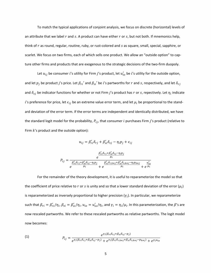
To match the typical applications of conjoint analysis, we focus on discrete (horizontal) levels of

an attribute that we label and . A product can have either or , but not both. If mnemonics help,

think of as round, regular, routine, ruby, or rust-colored and as square, small, special, sapphire, or

scarlet. We focus on two firms, each of which sells one product. We allow an “outside option” to cap-

ture other firms and products that are exogenous to the strategic decisions of the two-firm duopoly.

Let be consumer ’s utility for Firm ’s product, let be ’s utility for the outside option,

and let be product ’s price. Let ′ and ′ be ’s partworths for and , respectively, and let

and be indicator functions for whether or not Firm ’s product has or , repectively. Let indicate

’s preference for price, let be an extreme value error term, and let be proportional to the stand-

ard deviation of the error term. If the error terms are independent and identically distributed, we have

the standard logit model for the probability, , that consumer purchases Firm ’s product (relative to

Firm ’s product and the outside option):

= + − +

= + , , +

For the remainder of the theory development, it is useful to reparameterize the model so that

the coefficient of price relative to or is unity and so that a lower standard deviation of the error ( )

is reparameterized as inversely proportional to higher precision ( ). In particular, we reparameterize

such that = / , = / , = / , and = / . In this parameterization, the ’s are

now rescaled partworths. We refer to these rescaled partworths as relative partworths. The logit model

now becomes:

(1) = ( )( ) + ( , , ) +

6

If is the market volume (including volume due to the outside option), is the marginal cost

for product , and is Firm ’s fixed cost, and ( , , ) is the probability distribution over the rela-

tive partworths and precision (posterior if Bayesian), then the profit, , for Firm is given by:

(2) = − ( , , ) −

For the purposes of this paper we assume that does not depend on the quantity sold nor the choice of

or . These assumptions can be relaxed and do not reverse the basic intuition in this paper.

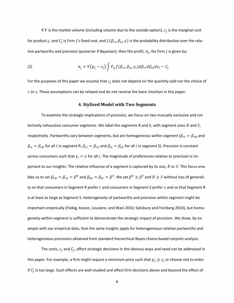
4. Stylized Model with Two Segments

To examine the strategic implications of precision, we focus on two mutually exclusive and col-

lectively exhaustive consumer segments. We label the segments R and S, with segment sizes and ,

respectively. Partworths vary between segments, but are homogeneous within segment ( = and = for all in segment R; = and = for all in segment S). Precision is constant

across consumers such that = for all . The magnitude of preferences relative to precision is im-

portant to our insights. The relative influence of a segment is captured by its size, or . This focus ena-

bles us to set = = and = = ℓ. We set ≥ ℓ and ≥ without loss of generali-

ty so that consumers in Segment R prefer and consumers in Segment S prefer and so that Segment R

is at least as large as Segment S. Heterogeneity of partworths and precision within segment might be

important empirically (Fiebig, Keane, Louviere, and Wasi 2010; Salisbury and Feinberg 2010), but homo-

geneity-within-segment is sufficient to demonstrate the strategic impact of precision. We show, by ex-

ample with our empirical data, that the same insights apply for heterogeneous relative partworths and

heterogeneous precisions obtained from standard hierarchical Bayes choice-based conjoint analysis.

The costs, and , affect strategic decisions in the obvious ways and need not be addressed in

this paper. For example, a firm might require a minimum price such that ≥ or choose not to enter

if is too large. Such effects are well-studied and affect firm decisions above and beyond the effect of

7

precision. For focus, we normalize to a unit market volume, set = 0, and roll marginal costs into

price by setting = 0.

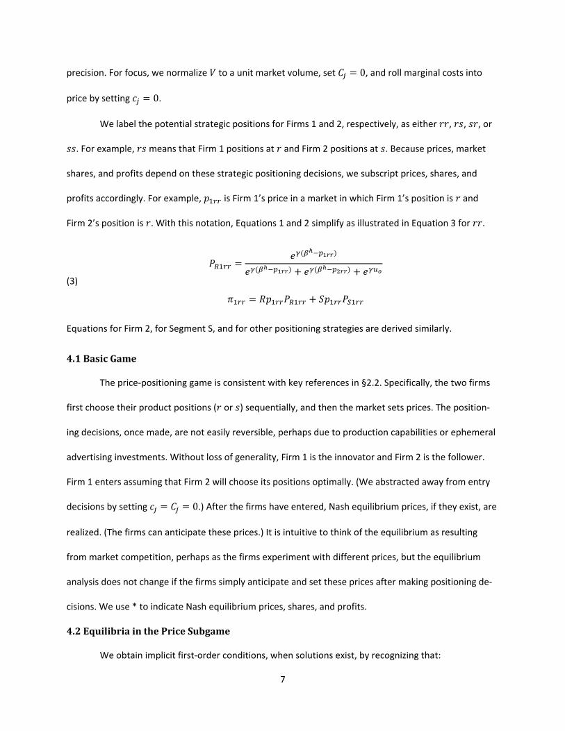
We label the potential strategic positions for Firms 1 and 2, respectively, as either , , , or

. For example, means that Firm 1 positions at and Firm 2 positions at . Because prices, market

shares, and profits depend on these strategic positioning decisions, we subscript prices, shares, and

profits accordingly. For example, is Firm 1’s price in a market in which Firm 1’s position is and

Firm 2’s position is . With this notation, Equations 1 and 2 simplify as illustrated in Equation 3 for .

(3)

= ( )( ) + ( ) +

= +

Equations for Firm 2, for Segment S, and for other positioning strategies are derived similarly.

4.1 Basic Game

The price-positioning game is consistent with key references in §2.2. Specifically, the two firms

first choose their product positions ( or ) sequentially, and then the market sets prices. The position-

ing decisions, once made, are not easily reversible, perhaps due to production capabilities or ephemeral

advertising investments. Without loss of generality, Firm 1 is the innovator and Firm 2 is the follower.

Firm 1 enters assuming that Firm 2 will choose its positions optimally. (We abstracted away from entry

decisions by setting = = 0.) After the firms have entered, Nash equilibrium prices, if they exist, are

realized. (The firms can anticipate these prices.) It is intuitive to think of the equilibrium as resulting

from market competition, perhaps as the firms experiment with different prices, but the equilibrium

analysis does not change if the firms simply anticipate and set these prices after making positioning de-

cisions. We use * to indicate Nash equilibrium prices, shares, and profits.

4.2 Equilibria in the Price Subgame

We obtain implicit first-order conditions, when solutions exist, by recognizing that:

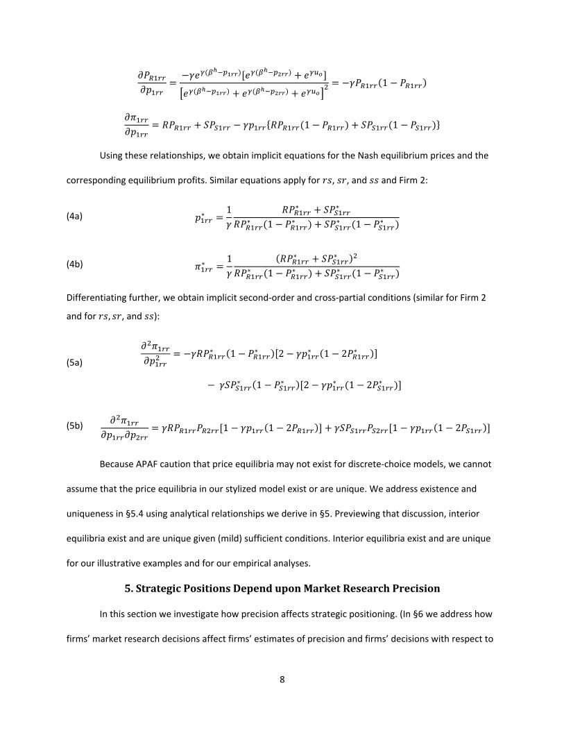
8

= − ( )[ ( ) + ]( ) + ( ) + = − (1 − ) = + − { (1 − ) + (1 − )}

Using these relationships, we obtain implicit equations for the Nash equilibrium prices and the

corresponding equilibrium profits. Similar equations apply for , , and and Firm 2:

(4a) ∗ = 1 ∗ + ∗∗ (1 − ∗ ) + ∗ (1 − ∗ )

(4b) ∗ = 1 ( ∗ + ∗ )∗ (1 − ∗ ) + ∗ (1 − ∗ ) Differentiating further, we obtain implicit second-order and cross-partial conditions (similar for Firm 2

and for , , and ):

(5a) = − ∗ (1 − ∗ )[2 − ∗ (1 − 2 ∗ )]

− ∗ (1 − ∗ )[2 − ∗ (1 − 2 ∗ )] (5b) = [1 − (1 − 2 )] + [1 − (1 − 2 )]

Because APAF caution that price equilibria may not exist for discrete-choice models, we cannot

assume that the price equilibria in our stylized model exist or are unique. We address existence and

uniqueness in §5.4 using analytical relationships we derive in §5. Previewing that discussion, interior

equilibria exist and are unique given (mild) sufficient conditions. Interior equilibria exist and are unique

for our illustrative examples and for our empirical analyses.

5. Strategic Positions Depend upon Market Research Precision

In this section we investigate how precision affects strategic positioning. (In §6 we address how

firms’ market research decisions affect firms’ estimates of precision and firms’ decisions with respect to

9

strategic positioning.) We first digress to explore the meaning of precision. Larger precision, , implies

the standard deviation of the error term, , is smaller and, hence, predictions are more precise. We

expect that higher-quality market research reports higher ’s, but higher-quality market research may

not eliminate prediction errors entirely. No matter how much a firm invests in market research, some

residual uncertainty will remain, perhaps because of random shocks, unmeasured product features, or

inherent stochasticity in consumer behavior. In notation, there is some true precision, , that de-

scribes how the market will react to changes in vs. positions and/or prices. To develop the machinery

to address strategic positioning and price equilibria, we examine how the firms would react if they knew

the true precision, . To simplify exposition in this section, we use rather than . We return to

notation in §6 when we examine the precision as reported by market research.

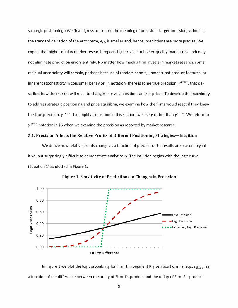
5.1. Precision Affects the Relative Profits of Different Positioning Strategies—Intuition

We derive how relative profits change as a function of precision. The results are reasonably intu-

itive, but surprisingly difficult to demonstrate analytically. The intuition begins with the logit curve

(Equation 1) as plotted in Figure 1.

Figure 1. Sensitivity of Predictions to Changes in Precision

In Figure 1 we plot the logit probability for Firm 1 in Segment R given positions , e.g., , as

a function of the difference between the utility of Firm 1’s product and the utility of Firm 2’s product

0.00

0.20

0.40

0.60

0.80

1.00

Logi

t Pro

babi

lity

Utility Difference

Low Precision

High Precision

Extremely High Precision

10

( − ). A zero difference (near where the curves meet) implies less than a 50% probability for

each firm because the outside option draws non-zero share. When precision is lower (solid black curve),

the logit probability is relatively insensitive to differences in utility and hence differences in price. For

lower precision, price competition will be less strong. The follower, Firm 2, may prefer to position for

the larger segment even if Firm 1 is already there. As precision increases, the logit curve becomes steep-

er and price competition increases. Firm 2 may decide to position in a different segment than Firm 1 to

reduce price competition. Finally, as precision gets extremely large, the logit curve is effectively a step-

function and price competition is extremely intense. For such large values of precision, the APAF suffi-

cient conditions are not satisfied, but price equilibria exist in our stylized model.

5.2. Precision Affects the Relative Profits of Different Positioning Strategies—Formal Results

We begin with the case of lower precision. Result 1 shows that extremely low precision implies

that price competition is so low that price moderation through differentiation does not offset the ad-

vantage of targeting the larger segment. Because the formal proofs are lengthy we provide a simple

sketch of the proof in the text. Details are in Appendix 3. (Appendix 3 is provided for review, otherwise it

will be available online.)

Result 1. For low precision ( → 0), Firm 2 prefers not to differentiate whenever Firm 1 positions

for the larger segment ( ∗ > ∗ ). However, Firm 1 would prefer that Firm 2 differentiate

( ∗ > ∗ ) and, if Firm 2 were to differentiate, Firm 1 would earn more profits than Firm 2

( ∗ > ∗ ).

Sketch of proof. The proof relies on the fact that, for low precision, the logit curve is relatively

flat. We use a Taylor’s series to linearize near = ℓ. All higher-order terms are proportional to pow-

ers of and, hence, disappear as → 0. The resulting price equilibrium is a one-variable fixed point

problem for which a unique solution exists. By symmetry, the shares at the fixed point are the same for

both firms and for both strategies ( and ). The Taylor’s series expansion provides an algebraic ex-

11

pression for ∗ − ∗ which has a minimum that is always positive as long as > . The proofs of

the other relative profit conditions follow similar steps and/or symmetry arguments.

Our second result examines the case where precision is high. The high precision result uses suf-

ficient conditions on the relative partworths and the outside option. Specifically, (1) if the partworth of

is larger than the outside option and (2) if the outside option is at least as large as the partworth of ,

then there is sufficient benefit to differentiating. With these conditions, market shares are sufficiently

sensitive to price for large . Differentiated positions moderate price competition enough to offset the

follower’s decision to target the smaller segment.

Result 2. Suppose is sufficiently larger than and ≥ ℓ. Then, there exists a sufficiently

large such that Firm 2 prefers to differentiate whenever Firm 1 positions for the larger segment

( ∗ > ∗ ). Differentiation earns more profits for Firm 1 than no differentiation ( ∗ > ∗ ),

and those profits are larger than the profits obtained by Firm 2 ( ∗ > ∗ ).

Sketch of proof. A lemma bounds equilibrium prices with an implicit relationship: ∗ ≤(1 − ∗ ) and ∗ ≤ (1 − ∗ ) for all . Similar equations hold for the -based prices. We

simplify the first-order conditions by recognizing that, for large and for ≥ ℓ, ∗ , ∗ , ∗ ,

and ∗ approach zero. The simplification implies ∗ ≅ (1 − ∗ ) and ∗ ≅ (1 − ∗ )

as → ∞. The solution to asymptotic equations imply finite prices and resulting profits. Specifically,

∗ → ( − ) and ∗ → ( − ) as → ∞. On the other hand, for the positions with > , ∗ → and ∗ < . This allows us to bound ∗ from above to a fixed value, which, in

turn, implies that ∗ → 0 and ∗ → 0 as → ∞. Because profits converge to a finite value and

profits converge to zero as gets large, we have shown that ∗ > ∗ and ∗ > ∗ . Finally, we

use > to show that ∗ > ∗ .

Together Results 1 and 2 establish that, if the innovator (Firm 1) targets the larger segment,

12

then the follower (Firm 2) will choose to differentiate ( ) when precision is high and will choose not to

differentiate ( ) when precision is low. All that remains is to show is that, in equilibrium, the innovator

will target the larger segment. While this may seem obvious, we need Results 3 and 4 to establish the

formal result. In Result 3, the inequality, ∗ > ∗ , uses the principle of optimality and the fact that > . The equalities in Result 3, ∗ = ∗ and ∗ = ∗ , follow from symmetry. Result 4 uses

details in the proof to Result 2 and symmetry to argue that Firm 1 prefers to .

Result 3. Among the undifferentiated strategies, both firms prefer to target the larger segment

( ∗ = ∗ > ∗ = ∗ ).

Result 4. Suppose is sufficiently larger than and > ℓ. Then, there exists a sufficiently

large such that Firm 1 prefers to differentiate by targeting the larger segment rather than the

smaller segment ( ∗ > ∗ ).

5.3. Equilibrium in Product Positions

Results 1 to 4 establish necessary and sufficient conditions to prove the following propositions.

The proofs in Appendix 3 rely on the inequalities and equalities established in Results 1-4.

Proposition 1. For low precision ( → 0), the innovator (Firm 1) targets the larger segment ( )

and the follower (Firm 2) chooses not to differentiate. It also targets the larger segment ( ).

Proposition 2. If is sufficiently larger than and if ≥ ℓ, then there exists a sufficiently

large such that the innovator (Firm 1) targets the larger segment ( ) and the follower chooses

to differentiate by targeting the smaller segment ( ).

In §6, we examine the implications of Proposition 1 for market research spending. For market

research implications it is sufficient that the positioning equilibrium is for small and for large .Because the profit functions are continuous (see also APAF), Propositions 1 and 2 and the Mean Value

Theorem imply that there exists a such the follower is indifferent between and . Numeri-

13

cally, for a wide variety of parameter values, the cutoff value is unique and ∗ − ∗ is monotonically

increasing in . However, although we can guarantee that a exists, we have not been able to

guarantee uniqueness analytically.

5.4. Existence and Uniqueness of the Price Equilibria

To prove that the price equilibria exist, we show that, for a compact set of potential prices, the

second-order conditions are negative. Because the proofs to Results 1 and 2 rely on interior solutions,

we also demonstrate that the first-order solutions are interior. To prove uniqueness, we show that the

absolute value of the second-order conditions (Equation 5a) exceeds the absolute value of the cross-

partial conditions (Equation 5b). Existence and uniqueness are shown for all positioning decisions.

The key to all proofs is a lemma, used by Result 2, that the equilibrium prices are bounded. For

example, for the positions: ∗ < (1 − ∗ ) and ∗ < (1 − ∗ ) for all . We define the

set of prices, and , such that the inequalities and/or equality holds (without the ∗’s). We show

the set is compact. These inequalities (without the ∗’s) guarantee that the second-order conditions hold,

possibly with a mild technical sufficient condition on vs. . The construction assures that the profit

functions are concave on the compact set and that the equilibrium is an interior solution. Similar reason-

ing implies that the cross-partial conditions hold, hence the equilibria are unique for each (with possi-

ble technical conditions on vs. ).

It would have been more satisfying to prove existence and uniqueness without restricting vs.

. Fortunately, (1) for a wide variety of parameter values both the second-order and cross-partial condi-

tions are satisfied and (2) the second-order and cross-partial conditions are satisfied asymptotically. We

have not been able to find a counterexample. (Computations available from the authors.) At minimum,

there exist (many) “markets” for which the price equilibria exist and are unique.

6. Implications for Market Research Spending

In this section we explore incentives to invest in higher-quality market research. We show that

14

the incentives are different for the innovator and the follower. In §5 we assumed that, even with the

best market research, the firm cannot eliminate uncertainty. There will always be residual uncertainty

due to random shocks, unmeasured product features, or inherent stochasticity in consumer behavior.

This residual uncertainty implies an upper bound on precision, which we labeled . The interesting

case is when is sufficiently large so that, at , the firms choose to differentiate ( ).

We assume the firm does not know and seeks to estimate it with market research. If the

firm invests in higher-quality market research, it estimates precision accurately ( ). If the firm cuts

corners and invests in lower-quality market research, it estimates precision (falsely) as . Based on

common practice, in which conjoint-analysis-based market simulators are used to estimate market

shares, we assume the, possibly naïve, firm believes its estimate of is accurate. In §6.3, we ad-

dress sophisticated firms, who might knowingly choose lower-quality market research. If the higher-

quality research eliminates all but the residual uncertainty, then = > . To focus on

precision, we assume that both the lower-quality market research and the higher-quality market re-

search estimate the relative partworths equally accurately. Because the assumption of accurate relative

partworths is an abstraction, we examine the empirical effect of market research quality on relative

partworths in §8.7.

6.1 Innovator’s Decision on Market Research

The innovator will choose to target the larger segment ( ) in both Propositions 1 and 2, thus we

have the following corollary. This corollary is consistent with recommendations in product development

(e.g., Urban and Hauser 1993, Ulrich and Eppinger 2004). Such texts advise innovators to use market

research to identify the best features, but also advise that the accuracy need only be sufficient for a

GO/NO-GO decision.

15

Corollary 1. The innovator (Firm 1) will choose to target the larger segment and this decision

does not depend upon true precision ( ). The innovator need not invest in the higher-quality

market research.

6.2. Naïve Follower’s Decision on Market Research

Precision matters to the follower because, in equilibrium, the follower’s optimal position de-

pends on . We first examine a naïve follower and then a sophisticated follower. If Firm 2 naively

underinvests in market research, and if < < , Firm 2 might make a strategic mis-

take and choose when the optimal positioning strategy is . Because this insight follows directly from

Propositions 1 and 2, we state the following corollary. (Recall that we assume the market sets equilibri-

um prices after positioning decisions are made.) By “appropriate investment,” we mean the case where

the investment in market research is less than the profit gained by Firm 2 for choosing a strategic posi-

tion of rather than when = . We provide formulae for “appropriate investment” in the next

subsection.

Corollary 2. If the follower (Firm 2) naively chooses to underinvest in market research such that

satisfies the conditions of Proposition 1 and if = satisfies the conditions of

Proposition 2, then the follower earns less profits than it could have earned with an appropriate

investment in higher-quality market research.

Some firms, such as Procter & Gamble, Chrysler, or General Motors are sophisticated and spend

substantially on conjoint analysis—sometimes tens of millions of dollars (e.g., Urban and Hauser 2004, p.

73). On the other hand, based on personal experience, many firms reduce research costs by using text-

only feature descriptions, less-sophisticated methods, and small sample sizes. Unfortunately, when firms

act falsely on , and when < < , the opportunity cost is not observable

because, even with the wrong strategic positioning, the firm still realizes positive profits.

16

Corollary 2 also illustrates cases where Firm 2 might make the right decision for the wrong rea-

sons. For example, if < = < , then Firm 2 will naively and correctly choose

even though it used lower-quality market research. Corollary 2 illustrates that there are instances, not

known a priori, when it is better to invest in higher-quality market research. Corollary 2 justifies the

substantial interest among academics and sophisticated practitioners in research to improve predictive

ability (precision).

6.3. Sophisticated Bayesian Follower’s Decision on Market Research

Not all firms are naïve. Sophisticated firms might anticipate that higher-quality conjoint analyses

resolve their uncertainty about precision. Such sophisticated firms would make optimal decisions on

whether or not to invest in higher-quality market research. Suppose that the follower has prior beliefs, ( ), about the true precision and can pay dollars to resolve that uncertainty. (For simplicity of

exposition, we normalize the cost of lower-quality market research to zero.) Suppose further that the

estimates of , ℓ, and are the same for both higher- and lower-quality market research, but only

the higher-quality research resolves . Because Firm 2 knows the relative partworths and Firm 2 is

sophisticated, Firm 2 can anticipate ∗ ( ) and ∗ ( ) for all values of .

If a sophisticated Firm 2 invests only in the lower-quality market research, it does not resolve ( ) and its expected profits are given by the following expression. Firm 2 chooses if the first term

in brackets is larger and if the second term in brackets is larger.

(6) [ ∗( ℎ)]= ∗ ( ) ( ) , ∗ ( ) ( )

On the other hand, if higher-quality market research resolves ( ), then, for an observed

, Firm 2 will choose if ∗ ( ) < ∗ ( ), if ∗ ( ) > ∗ ( ), and choose

randomly if ∗ ( ) = ∗ ( ). If Δ ( ) = 1 indicates it is optimal for Firm 2 to differenti-

17

ate for an observed and if Δ ( ) = 0 indicates it is optimal not to differentiate, then Firm 2’s

expected profits are given by:

(7) [ ∗(ℎ ℎ ℎ)]= { ∗ ( )Δ ( ) + ∗ ( )[1 − Δ ( )]} ( ) −

To decide on whether or not to invest in the higher-quality market research, Firm 2 need only compare

the profits given by Equations 6 and 7. Although the notation in Equations 6 and 7 is cumbersome, the

illustrative example in §7 illustrates Firm 2’s decision process simply and intuitively.

Finally, we note that we would have obtained the same insight for sophisticated firms had we

formulated a three-stage game in which the firms choose market research anticipating strategic posi-

tioning and then choose positioning anticipating price. We did not formulate the three-stage game be-

cause we wanted to compare naïve and sophisticated market research decisions. Our experience sug-

gests that many firms are naïve. Many firms make “gut” decisions on conjoint analysis investments that

may or may not be optimal.

7. Illustrative Example

We illustrate the results, propositions, and corollaries with a numerical example in which = 2, ℓ = 1, = 1, and = 0.55. We obtain the fixed-point equilibria by simple iteration. In all

cases, we check that the second-order and cross-partial conditions are satisfied.

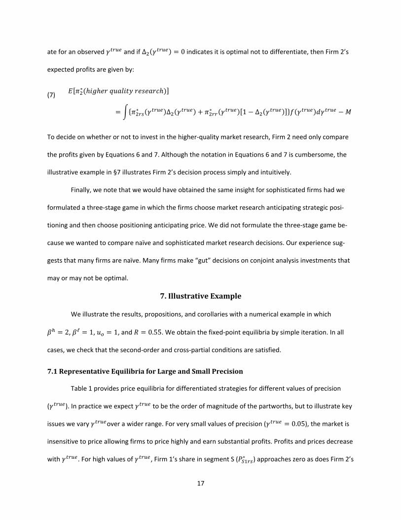
7.1 Representative Equilibria for Large and Small Precision

Table 1 provides price equilibria for differentiated strategies for different values of precision

( ). In practice we expect to be the order of magnitude of the partworths, but to illustrate key

issues we vary over a wider range. For very small values of precision ( = 0.05), the market is

insensitive to price allowing firms to price highly and earn substantial profits. Profits and prices decrease

with . For high values of , Firm 1’s share in segment S ( ∗ ) approaches zero as does Firm 2’s

18

share in Segment R ( ∗ ). The market is truly segmented for such high values of precision.

Table 1. Prices, Shares, Profits, and Second-order Conditions: Differentiated Market

Prices Shares in Segment R

Shares in Segment S Profits Second Order

Conditions

∗ ∗ ∗ ∗ ∗ ∗ ∗ ∗ ∗

∗

0.05 24.625 24.603 0.192 0.183 0.183 0.192 4.622 4.600 -0.009 -0.009 0.50 2.588 2.564 0.261 0.160 0.158 0.264 0.556 0.531 -0.103 -0.107 1.0 1.418 1.394 0.345 0.130 0.126 0.352 0.350 0.320 -0.137 -0.144 2.0 0.923 0.905 0.501 0.070 0.067 0.511 0.282 0.243 -0.491 -0.573 3.0 0.817 0.807 0.614 0.031 0.030 0.621 0.287 0.240 -0.808 -0.589 4.0 0.787 0.783 0.692 0.013 0.013 0.696 0.304 0.251 -1.200 -1.481 5.0 0.779 0.778 0.747 0.005 0.005 0.747 0.322 0.264 -1.639 -2.018 10 0.805 0.805 0.876 0.000 0.000 0.876 0.388 0.317 -3.938 -4.815 20 0.861 0.861 0.942 0.000 0.000 0.942 0.446 0.365 -8.477 -10.36

200 0.974 0.974 0.995 0.000 0.000 0.995 0.533 0.436 -89.54 -109.4

Table 2. Prices, Shares, Profits, and Relative Profits: Undifferentiated Market

Prices Shares in Segment R

Shares in Segment S Profits Relative

Profits

∗ ∗ ∗ ∗ ∗ ∗ ∗ ∗ ∗ − ∗

∗ −∗ 0.05 24.619 24.619 0.190 0.190 0.184 0.184 4.618 4.618 0.004 -0.018 0.50 2.553 2.553 0.240 0.240 0.179 0.179 0.542 0.542 0.014 -0.011 1.0 1.341 1.341 0.294 0.294 0.172 0.172 0.320 0.320 0.030 0.0004 2.0 0.744 0.744 0.385 0.385 0.156 0.156 0.209 0.209 0.072 0.034 3.0 0.539 0.539 0.444 0.444 0.142 0.142 0.166 0.166 0.121 0.074 4.0 0.425 0.425 0.476 0.476 0.134 0.134 0.137 0.137 0.167 0.114 5.0 0.349 0.349 0.491 0.491 0.130 0.130 0.114 0.114 0.208 0.150 10 0.177 0.177 0.500 0.500 0.127 0.127 0.059 0.059 0.329 0.258 20 0.089 0.089 0.500 0.500 0.127 0.127 0.029 0.029 0.416 0.335

200 0.009 0.009 0.500 0.500 0.127 0.127 0.003 0.003 0.530 0.433

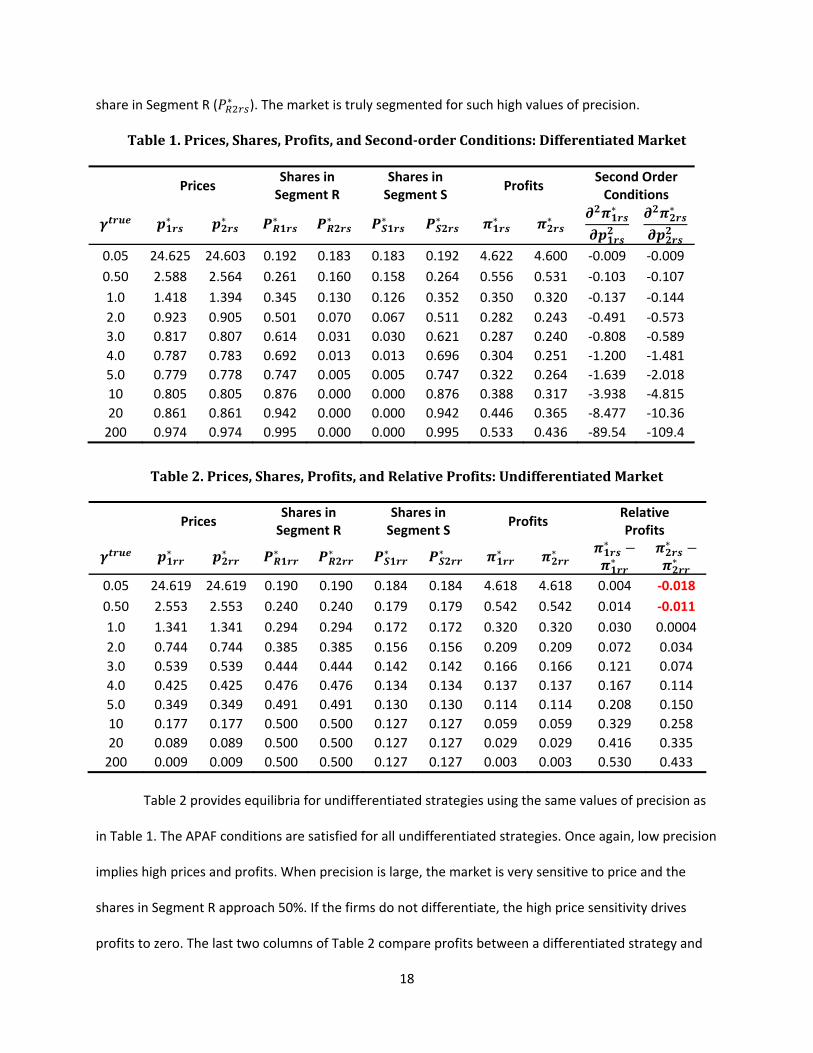
Table 2 provides equilibria for undifferentiated strategies using the same values of precision as

in Table 1. The APAF conditions are satisfied for all undifferentiated strategies. Once again, low precision

implies high prices and profits. When precision is large, the market is very sensitive to price and the

shares in Segment R approach 50%. If the firms do not differentiate, the high price sensitivity drives

profits to zero. The last two columns of Table 2 compare profits between a differentiated strategy and

19

an undifferentiated strategy. For low precision ( = 0.05and 0.50), strategy is more profitable

than for Firm 2. This is shown in a red bold font.

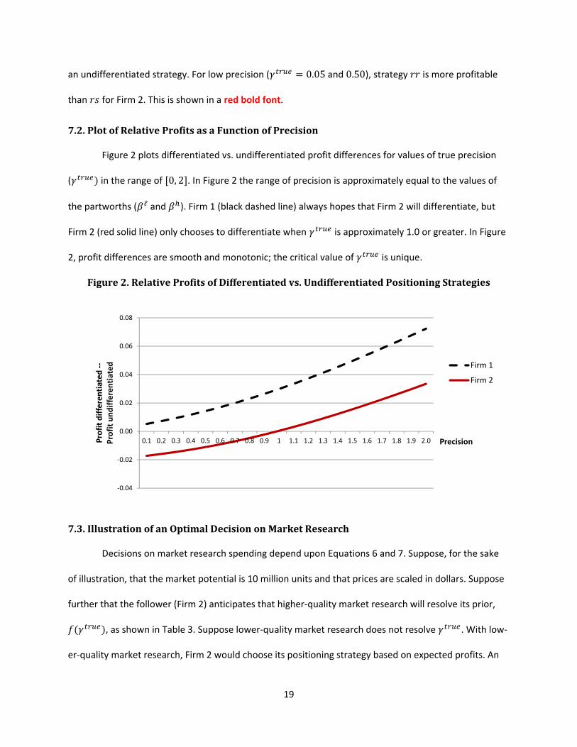
7.2. Plot of Relative Profits as a Function of Precision

Figure 2 plots differentiated vs. undifferentiated profit differences for values of true precision

( ) in the range of [0, 2]. In Figure 2 the range of precision is approximately equal to the values of

the partworths ( ℓ and ). Firm 1 (black dashed line) always hopes that Firm 2 will differentiate, but

Firm 2 (red solid line) only chooses to differentiate when is approximately 1.0 or greater. In Figure

2, profit differences are smooth and monotonic; the critical value of is unique.

Figure 2. Relative Profits of Differentiated vs. Undifferentiated Positioning Strategies

7.3. Illustration of an Optimal Decision on Market Research

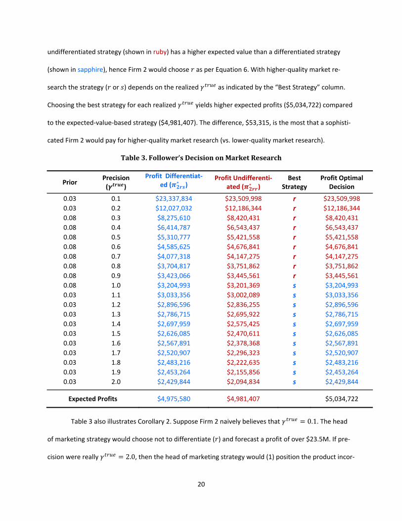
Decisions on market research spending depend upon Equations 6 and 7. Suppose, for the sake

of illustration, that the market potential is 10 million units and that prices are scaled in dollars. Suppose

further that the follower (Firm 2) anticipates that higher-quality market research will resolve its prior, ( ), as shown in Table 3. Suppose lower-quality market research does not resolve . With low-

er-quality market research, Firm 2 would choose its positioning strategy based on expected profits. An

-0.04

-0.02

0.00

0.02

0.04

0.06

0.08

0.1 0.2 0.3 0.4 0.5 0.6 0.7 0.8 0.9 1 1.1 1.2 1.3 1.4 1.5 1.6 1.7 1.8 1.9 2.0Prof

it di

ffere

ntia

ted

--Pr

ofit

undi

ffere

ntia

ted

Precision

Firm 1

Firm 2

20

undifferentiated strategy (shown in ruby) has a higher expected value than a differentiated strategy

(shown in sapphire), hence Firm 2 would choose as per Equation 6. With higher-quality market re-

search the strategy ( or ) depends on the realized as indicated by the “Best Strategy” column.

Choosing the best strategy for each realized yields higher expected profits ($5,034,722) compared

to the expected-value-based strategy ($4,981,407). The difference, $53,315, is the most that a sophisti-

cated Firm 2 would pay for higher-quality market research (vs. lower-quality market research).

Table 3. Follower’s Decision on Market Research

Prior Precision ( )

Profit Differentiat-ed ( ∗ )

Profit Undifferenti-ated ( ∗ )

Best Strategy

Profit Optimal Decision

0.03 0.1 $23,337,834 $23,509,998 r $23,509,998 0.03 0.2 $12,027,032 $12,186,344 r $12,186,344 0.08 0.3 $8,275,610 $8,420,431 r $8,420,431 0.08 0.4 $6,414,787 $6,543,437 r $6,543,437 0.08 0.5 $5,310,777 $5,421,558 r $5,421,558 0.08 0.6 $4,585,625 $4,676,841 r $4,676,841 0.08 0.7 $4,077,318 $4,147,275 r $4,147,275 0.08 0.8 $3,704,817 $3,751,862 r $3,751,862 0.08 0.9 $3,423,066 $3,445,561 r $3,445,561 0.08 1.0 $3,204,993 $3,201,369 s $3,204,993 0.03 1.1 $3,033,356 $3,002,089 s $3,033,356 0.03 1.2 $2,896,596 $2,836,255 s $2,896,596 0.03 1.3 $2,786,715 $2,695,922 s $2,786,715 0.03 1.4 $2,697,959 $2,575,425 s $2,697,959 0.03 1.5 $2,626,085 $2,470,611 s $2,626,085 0.03 1.6 $2,567,891 $2,378,368 s $2,567,891 0.03 1.7 $2,520,907 $2,296,323 s $2,520,907 0.03 1.8 $2,483,216 $2,222,635 s $2,483,216 0.03 1.9 $2,453,264 $2,155,856 s $2,453,264 0.03 2.0 $2,429,844 $2,094,834 s $2,429,844

Expected Profits $4,975,580 $4,981,407 $5,034,722

Table 3 also illustrates Corollary 2. Suppose Firm 2 naively believes that = 0.1. The head

of marketing strategy would choose not to differentiate ( ) and forecast a profit of over $23.5M. If pre-

cision were really = 2.0, then the head of marketing strategy would (1) position the product incor-

21

rectly ( rather than ), (2) bear an opportunity cost of $335,010, and (3) not realize anywhere near the

anticipated equilibrium price (not shown in Table 3) or the forecast profit ($2.1M vs. $23.5M).

8. Empirical Example: Smartwatches

The quality of market research affects strategic positioning in the stylized model, but we would

like to be confident that the quality of market research affects strategic positioning in real applications.

To address this question, we undertook empirical studies to address whether:

• higher-quality market research can increase precision, and

• hierarchical-Bayes choice-based conjoint analyses (HB CBC) can produce results analogous to

those derived with the stylized model.

8.1. Empirical Data from Hierarchical Bayes Choice-Based Conjoint Analyses

We designed higher- and lower-quality studies to match typical empirical practice in conjoint

analysis. Our sample was drawn from a professional panel,1 our design of sixteen choice sets for estima-

tion (and two for validation) with three profiles per choice set is typical, and our analysis of the data

with hierarchical Bayes is standard (Sawtooth Software 2015b). We followed standard survey design

principles including extensive pretesting (28 respondents in the higher-quality study and 38 in the lower-

quality study) to assure that (1) the questions, features, and tasks were easy to understand and (2) that

the manipulation of research quality between respondents was not subject to demand artifacts. We

screened the sample so that respondents expressed interest in the category, were based in the US, aged

20-69, and agreed to informed consent as required by our internal review boards. Based on these data,

HB CBC provides an empirical distribution of relative partworths and precisions that vary by respondent.

The product category was smartwatches. We abstracted from the large number of features in

smartwatches to focus on case color (silver or gold), watch face (round or rectangular), watch band

1 Peanut Labs is an international panel with 15 million pre-screened panelists from 36 countries. Their many corporate clients cumulatively gather approximately 450,000 completed surveys per month. Peanut Labs is a member of the ARF, CASRO, ESOMAR, and the MRA and has won many awards: web.peanutlabs.com.

22

(black leather, brown leather, or matching metal color), and price ($299 to $449). Following industry

practice, we held all other features constant, including brand, so that we could estimate the relative

tradeoffs among the features that we varied. Our focus on three features was sufficient to test the gen-

eralizability of the stylized model; an industry study might vary more features.

8.2. Higher-Quality Study with Animations, Realistic Pictures, and Incentive Alignment

After the screening questions, respondents saw an animated video describing the smartwatch

category, the smartwatch features, and the CBC task.2 Respondents completed a training task (not used

in estimation), then saw an animated video to induce incentive alignment (e.g., Ding 2007; Ding, Grewal,

and Liechty 2005; Ding, et al. 2011). Respondents were told that some respondents (1 in 500) would

receive a smartwatch and/or cash with a combined value of $500—based on their answers to the sur-

vey. See Figure 3. To enhance the effect of incentives, we screened out respondents who already owned

a smartwatch. Such screening is reasonable for our research purpose; the same screening was applied in

the lower-quality study. Respondents in both studies received standard panel incentives for participat-

ing in the study.

We used the dual-response task shown in Figure 4. Each respondent chose among realistic im-

ages of three smartwatches and then indicated whether or not he or she would purchase the smart-

watch. To make the images more realistic, the respondent could toggle among a detailed view, a top

view, and an app view as shown on the right side of Figure 4.

8.3. Lower-Quality Study

In the lower-quality study, respondents did not see the training and incentive-alignment videos,

did not receive an incentive-alignment promise, saw only simple drawings of smartwatches, could not

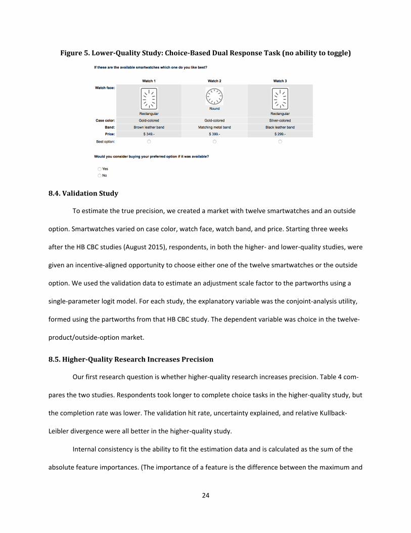
toggle among views, and were not informed that other features were to be held constant. See Figure 5.

All other aspects of the study remained the same.

2 The training video is available at https://www.youtube.com/watch?v=oji_bw_oxTU&rel=0. The incentive-alignment video is available at https://www.youtube.com/watch?v=DBLPfRJo2Ho&rel=0.

23

Figure 3. Incentive Alignment Screenshot from the Higher-Quality Study

Figure 4. Higher-Quality Study: Choice-Based Dual Response Task & Toggled Examples

24

Figure 5. Lower-Quality Study: Choice-Based Dual Response Task (no ability to toggle)

8.4. Validation Study

To estimate the true precision, we created a market with twelve smartwatches and an outside

option. Smartwatches varied on case color, watch face, watch band, and price. Starting three weeks

after the HB CBC studies (August 2015), respondents, in both the higher- and lower-quality studies, were

given an incentive-aligned opportunity to choose either one of the twelve smartwatches or the outside

option. We used the validation data to estimate an adjustment scale factor to the partworths using a

single-parameter logit model. For each study, the explanatory variable was the conjoint-analysis utility,

formed using the partworths from that HB CBC study. The dependent variable was choice in the twelve-

product/outside-option market.

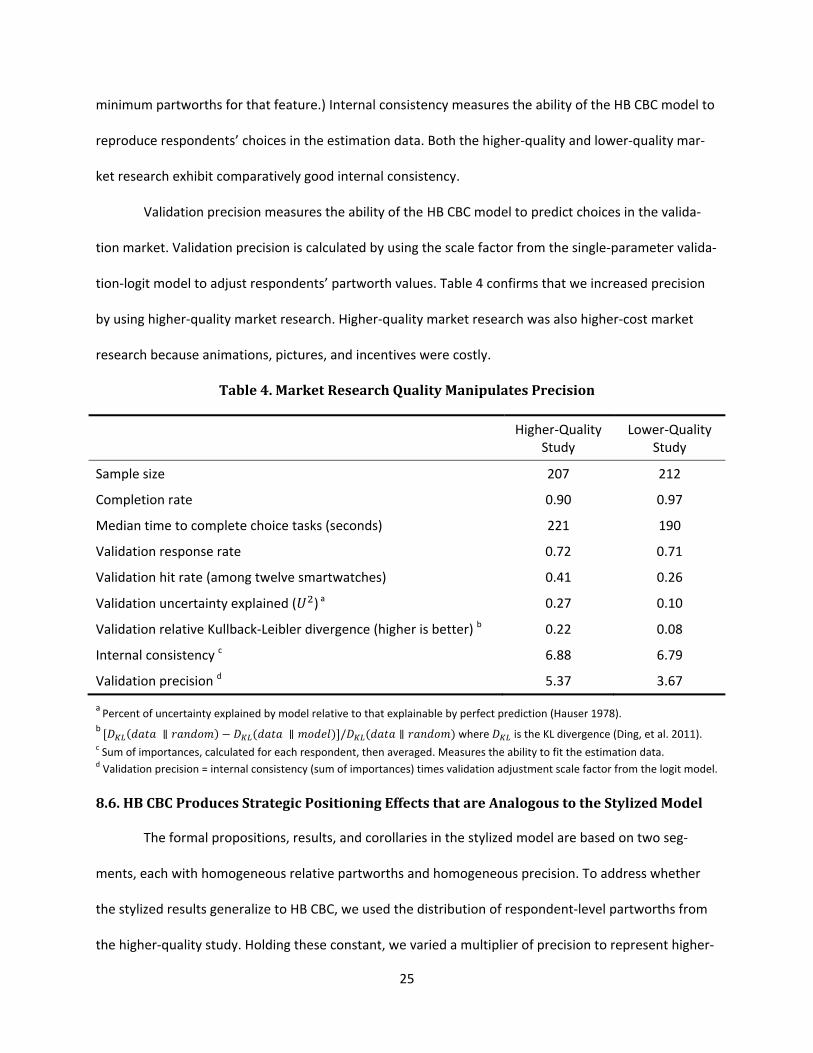
8.5. Higher-Quality Research Increases Precision

Our first research question is whether higher-quality research increases precision. Table 4 com-

pares the two studies. Respondents took longer to complete choice tasks in the higher-quality study, but

the completion rate was lower. The validation hit rate, uncertainty explained, and relative Kullback-

Leibler divergence were all better in the higher-quality study.

Internal consistency is the ability to fit the estimation data and is calculated as the sum of the

absolute feature importances. (The importance of a feature is the difference between the maximum and

25

minimum partworths for that feature.) Internal consistency measures the ability of the HB CBC model to

reproduce respondents’ choices in the estimation data. Both the higher-quality and lower-quality mar-

ket research exhibit comparatively good internal consistency.

Validation precision measures the ability of the HB CBC model to predict choices in the valida-

tion market. Validation precision is calculated by using the scale factor from the single-parameter valida-

tion-logit model to adjust respondents’ partworth values. Table 4 confirms that we increased precision

by using higher-quality market research. Higher-quality market research was also higher-cost market

research because animations, pictures, and incentives were costly.

Table 4. Market Research Quality Manipulates Precision

Higher-Quality Study

Lower-Quality Study

Sample size 207 212

Completion rate 0.90 0.97

Median time to complete choice tasks (seconds) 221 190

Validation response rate 0.72 0.71

Validation hit rate (among twelve smartwatches) 0.41 0.26

Validation uncertainty explained ( ) a 0.27 0.10

Validation relative Kullback-Leibler divergence (higher is better) b 0.22 0.08

Internal consistency c 6.88 6.79

Validation precision d 5.37 3.67

a Percent of uncertainty explained by model relative to that explainable by perfect prediction (Hauser 1978). b [ ( ∥ ) − ( ∥ )]/ ( ∥ ) where is the KL divergence (Ding, et al. 2011). c Sum of importances, calculated for each respondent, then averaged. Measures the ability to fit the estimation data. d Validation precision = internal consistency (sum of importances) times validation adjustment scale factor from the logit model.

8.6. HB CBC Produces Strategic Positioning Effects that are Analogous to the Stylized Model

The formal propositions, results, and corollaries in the stylized model are based on two seg-

ments, each with homogeneous relative partworths and homogeneous precision. To address whether

the stylized results generalize to HB CBC, we used the distribution of respondent-level partworths from

the higher-quality study. Holding these constant, we varied a multiplier of precision to represent higher-

26

and lower-precision markets and examined positioning decisions for case color (silver vs. gold). Using

only one of the studies enabled us to focus on precision. Purely for the sake of illustration, we assume

that case-color decisions are difficult to reverse. We obtained stable price equilibria with a grid search.

In §8.7 we examine relative partworth differences between the studies.

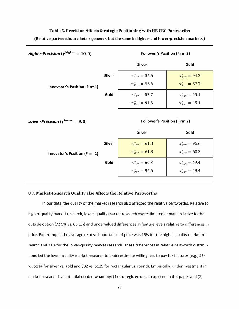
Table 5 summarizes the results with unit demand and zero costs. The equilibria exist and appear

to be unique. Because more respondents preferred silver to gold (75.4%) than vice versa, the analogy to

the stylized model is = silver even though “ ” is mnemonically cumbersome for silver. For illustration,

we chose values of precision near the strategic cutoff point. As precision decreased from = 10.0

to = 9.0, the positioning equilibrium shifted from differentiated positions (silver, gold) to undif-

ferentiated positions (silver, silver). If we assume that the market is 10 million units, then positioning

based on misestimating would result in an $11 million opportunity loss. These volumes are not unrea-

sonable: estimates of Apple Watch sales are 3.6 million units per quarter (Wakabayashi 2015).

We obtained similar results when we repeated the analysis for watch face (rectangular vs.

round) and watch strap (black vs. brown or other combinations). Precision had a similar effect when we

used self-explicated preference measurement (data from Putnam-Farr 2015). In all of these empirical

tests, the market always shifted from differentiated to undifferentiated as precision decreased below a

critical value. We conclude that there are examples where the stylized theory applies to empirical data

with heterogeneous relative partworths and heterogeneous precisions.

Consistent with theory, equilibria for lower-quality market research also depended on precision.

The positioning equilibrium for lower-quality market research was differentiated (silver, gold) when ≥ 5.0, but changed to undifferentiated (silver, silver) when ≤ 4.5. (For illustration, we

chose values of near the cutoff point.) Predicted profits and price were consistent with Tables 1 & 2,

that is, lower precision implied higher (and unrealized) profits and prices.

27

Table 5. Precision Affects Strategic Positioning with HB CBC Partworths

(Relative partworths are heterogeneous, but the same in higher- and lower-precision markets.)

Higher-Precision ( = . ) Follower’s Position (Firm 2)

Silver Gold

Innovator’s Position (Firm1)

Silver ∗ = 56.6 ∗ = 56.6

∗ = 94.3 ∗ = 57.7

Gold ∗ = 57.7 ∗ = 94.3

∗ = 45.1 ∗ = 45.1

Lower-Precision ( = . ) Follower’s Position (Firm 2)

Silver Gold

Innovator’s Position (Firm 1)

Silver ∗ = 61.8 ∗ = 61.8

∗ = 96.6 ∗ = 60.3

Gold ∗ = 60.3 ∗ = 96.6

∗ = 49.4 ∗ = 49.4

8.7. Market-Research Quality also Affects the Relative Partworths

In our data, the quality of the market research also affected the relative partworths. Relative to

higher-quality market research, lower-quality market research overestimated demand relative to the

outside option (72.9% vs. 65.1%) and undervalued differences in feature levels relative to differences in

price. For example, the average relative importance of price was 15% for the higher-quality market re-

search and 21% for the lower-quality market research. These differences in relative partworth distribu-

tions led the lower-quality market research to underestimate willingness to pay for features (e.g., $64

vs. $114 for silver vs. gold and $32 vs. $129 for rectangular vs. round). Empirically, underinvestment in

market research is a potential double-whammy: (1) strategic errors as explored in this paper and (2)

28

tactical errors due to misestimating relative partworths and willingness to pay for features.

8.8. Optimal Positioning in the Real Smartwatch Market

The higher-quality market research attempted to reproduce the best industry practice, thus we

examine the implications of our data for differentiation on smartwatch case color. The observed higher-

quality precision ( = 5.37) is below the cutoff for differentiation ( ≅ 9.5), suggesting that

smartwatch manufacturers should not differentiate on case color. When we examined the real market,

we saw that the first smartwatches introduced were mainly available in silver. For example, although

the Apple Watch was first available in both stainless steel (silver) and 18-karat gold (gold), Apple’s 18-

karat gold differed from “silver” on more than just color—for example, it was offered at a substantially

higher price ($15,000). Both manufacturers now offer both colors. Apple recently introduced a gold-

colored case. The Moto 360 is available in silver, gold, and black case colors. The smartwatch market

appears to differentiate on features other than case color—features held constant in both of our con-

joint analysis studies.

Although neither the higher-quality nor the lower-quality market research implied differentia-

tion on case color, this does not undermine the theory. In fact, it illustrates the case where << . The true precision is a reflection of whether the features we tested were appropriate

for differentiation in the smartwatch market. In the real smartwatch market, there are likely other viable

features for differentiation that overwhelm case color in consumer choice. Operating system (iOS vs.

Android) might be one of them. Operating system has an additional advantage for positioning because it

is more difficult to reverse than case color. Had the true precision been different and had case color

been difficult to reverse, then case color might have been a viable candidate for differentiation.

9. Discussion and Summary

Precision matters strategically. Formal analyses, numerical examples, and empirical data all illus-

trate that a follower’s decision about strategic positioning depends critically on investments in the quali-

29

ty of market research. Higher-quality market research enables followers to make the right positioning

decisions and avoid strategic mistakes. Innovators, who need only identify the best features for the ap-

propriate target segment, may choose to invest in lower-quality market research (if the relative part-

worths remain the same).

In our analyses, we abstracted from marginal and fixed costs because these effects are well-

studied and do not change the insights relative to precision. Likewise, it is clear that, if lower-quality

market research misidentifies the partworths, then both the innovator and the follower will make tacti-

cal errors in product design. Such errors are well-studied. We propose an additional motivation for high-

er-quality market research—strategic positioning. It might surprise many that, even if the relative part-

worths are unbiased, precision can affect strategic positioning.

Finally, a firm need not always invest in the highest-quality research to make correct strategic

decisions. For every market there is a critical precision, , above which the follower should differ-

entiate. The follower must only assure that it invests sufficiently in market research, as given by Equa-

tions 6 and 7, to know whether precision is above the cutoff. These critical values help firms decide

which of the many published improvements in conjoint analysis are worth the investment. We believe

many will pass the test.

30

References

Aksoy-Pierson M, Allon G, Federgruen A (2013) Price competition under mixed multinomial logit de-

mand functions. Management Science 59 (8): 1817-1835.

Andrews RL, Ansari A, Currim I (2002) Hierarchical Bayes versus finite mixture conjoint analysis models:

A comparison of fit, prediction, and partworth recovery. Journal of Marketing Research

39(1):87-98.

Caplin A, Nalebuff B (1991) Aggregation and imperfect competition: On the existence of equilibrium.

Econometrica 59(1):25-59.

Choi SC, DeSarbo WS (1994) A conjoint simulation model incorporating short-run price competition.

Journal of Product Innovation Management 11:451-459.

Choi SC, DeSarbo WS, Harker PT (1990) Product positioning under price competition. Management Sci-

ence 36(2):175-199.

d’Aspremont C, Gabszewicz JJ, Thisse JF (1979) On Hotelling’s stability in competition. Econometrica

47(5), (September):1145-1150.

de Palma A, Ginsburgh V, Papageorgiou YY, Thisse JF (1985) The principle of minimum differentiation

holds under sufficient heterogeneity. Econometrica 53(4):767-781.

Ding, M. (2007) An incentive-aligned mechanism for conjoint analysis. Journal of Marketing Research,

54, (May), 214-223.

Ding, M., R. Grewal, J. Liechty (2005) Incentive-aligned conjoint analysis. Journal of Marketing Research

42, (February), 67–82.

Ding, M., J. R. Hauser, S. Dong, D. Dzyabura, Z. Yang, C. Su, S. Gaskin (2011) Unstructured direct elicita-

tion of decision rules. Journal of Marketing Research 48, (February), 116-127.

Eaton B, Lipsey RG (1975) The principle of minimum differentiation reconsidered: Some new develop-

ments in the theory of spatial competition. Review of Economic Studies 42(129):27-50.

Eaton B, Wooders MH (1985) Sophisticated entry in a model of spatial competition. Rand Journal of

Economics 16(2)(Summer):282-297.

Economides N (1984) The principle of minimum differentiation revisited. European Econ Review 24:1-24.

Economides N (1986) Nash equilibrium in duopoly with products defined by two characteristics. Rand

Journal of Economics, 17(3):431-439.

Evgeniou T, Pontil M, Toubia O (2007) A convex optimization approach to modeling heterogeneity in

conjoint estimation. Marketing Science 26(6):805-818.

Fiebig DG, Keane MP, Louviere J, Wasi N (2010) The generalized multinomial logit model: Accounting for

31

scale and coefficient heterogeneity. Marketing Science 29(3):393-421.

Graitson D (1982) Spatial competition a la Hotelling: A selective survey. The Journal of Industrial Eco-

nomics 31(1-2)(September-December):13-25.

Hauser JR (1978) Testing the accuracy, usefulness and significance of probabilistic models: An infor-

mation theoretic approach. Operations Research 26(3):406-421.

Hauser JR (1988) Competitive price and positioning strategies. Marketing Science 7(1):76-91.

Hotelling H (1929) Stability in competition. The Economic Journal 39:41-57.

Irmen A, Thisse JF (1998) Competition in multi-characteristics spaces: Hotelling was almost right. Journal

of Economic Theory 78:76-102.

Johnson JP, Myatt DP (2006) On the simple economics of advertising, marketing, and product design.

American Economic Review 96(3):756-784.

Luo L, Kannan PK, Ratchford BT (2007) New product development under channel acceptance. Marketing

Science 26(2):149–163.

Novshek W (1980) Equilibrium in simple spatial (or differentiated product) models. Journal of Economic

Theory 22:313-326.

Putnam-Farr E (2015) The effect of message framing on initial choices, satisfaction, and ongoing en-

gagement. PhD Thesis, MIT, Cambridge, MA.

Rhee BD, de Palma A, Fornell C, Thisse JF (1992) Restoring the principle of minimum differentiation in

product positioning. Journal of Economics & Management Strategy 1(3):475-505.

Rossi PE, Allenby GM (2003) Bayesian Statistics and marketing. Marketing Science 23(3):304-328.

Sajeesh S, Raju JS (2010) Positioning and pricing in a variety seeking market. Management Science

56(6):949-61.

Salisbury LC, Feinberg FM (2010) Alleviating the constant stochastic variance assumption in decision

research: Theory, measurement, and experimental test. Marketing Science 29(1):1-17.

Sawtooth Software (2015a) http://www.sawtoothsoftware.com/products/conjoint-choice-

analysis/conjoint-analysis-software.

Sawtooth Software (2015b) http://www.sawtoothsoftware.com/download/Conjoint_Report_2015.pdf.

Shaked A, Sutton J (1982) Relaxing price competition through product differentiation. Review of Eco-

nomic Studies 49:3-13.

Shilony Y (1981) Hotelling’s competition with general customer distribution. Economic Letters 8:39-45.

Toubia O, Hauser JR, Garcia R (2007) Probabilistic polyhedral methods for adaptive choice-based conjoint

analysis: Theory and application. Marketing Science 26(5):596-610.

32

Ulrich KT, Eppinger SD (2004) Product Design and Development, 3E. McGraw-Hill: New York NY.

Urban GL, Hauser JR (1993) Design and Marketing of New Products. Prentice-Hall: Englewood Cliffs, NJ.

Urban GL, Hauser JR (2004) ’Listening-in’ to find and explore new combinations of customer needs.

Journal of Marketing 68 (April), 72-87.

Wakabayahi, D (2015) Apple Watch Sales May be Pretty Good After All. WSJ.D,

http://blogs.wsj.com/digits/2015/08/27/apple-watch-sales-may-be-pretty-good-after-all/.

Zeithammer R, Thomadsen R (2012) Vertical differentiation with variety-seeking consumers. Manage-

ment Science 59(2):390-401.

Additional References for Online Appendix 2 Aribarg A, Arora N, Kang MY (2010) Predicting joint choice using individual data. Marketing Science

29(1):139-157. Arora N, Henderson T, Liu Q (2011) Noncompensatory dyadic choices. Marketing Science 30(6):1028-47. Cui D, Curry D (2005) Prediction in marketing using the support vector machine. Marketing Science

24(4):595-615. Dyachenko T, Reczek RW, Allenby GM (2014) Models of sequential evaluation in best-worst choice tasks.

Marketing Science 33(6):828-848. Dzyabura D, Hauser JR (2011) Active machine learning for consideration heuristics. Marketing Science

30(5):801-819. Gilbride TJ, Allenby GM (2004) A choice model with conjunctive, disjunctive, and compensatory screen-

ing rules. Marketing Science 23(3):391-406. Gilbride TJ, Allenby GM (2006) Estimating heterogeneous EBA and economic screening rule choice mod-

els. Marketing Science 25(5):494-509. Gilbride TJ, Lenk PJ, Brazell JD (2008) Market share constraints and the loss function in choice-based

conjoint analysis. Marketing Science 27(6):995-1011. Hauser JR, Toubia O (2005) The impact of utility balance and endogeneity in conjoint analysis. Marketing

Science 24(3):498-507. Iyengar R, Jedidi K (2012) A conjoint model of quantity discounts. Marketing Science 31(2):334-350. Jedidi K, Jagpal S, Manchanda P (2003) Measuring heterogeneous reservation prices for product bun-

dles. Marketing Science 22(1):107-130. Kohli R, Jedidi K (2007) Representation and inference of lexicographic preference models and their vari-

ants. Marketing Science 26(3):380-399. Liu Q, Arora N (2011) Efficient choice designs for a consider-then-choose model. Marketing Science

30(2):321-338. Liu Q, Otter T, Allenby GM (2007) Investigating endogeneity bias in marketing. Marketing Science.

26(5):642-650. Park JH, MacLachlan DL (2008) Estimating willingness to pay with exaggeration bias-corrected contin-

gent valuation method. Marketing Science 27(4):691-698. Swait J, Erdem T (2007) Brand effects on choice and choice set formation under uncertainty. Marketing

33

Science 26(5):679-697. Toubia O, de Jong MG, Stieger D, Fuller J (2012) Measuring consumer preferences using conjoint poker.

Marketing Science 31(1):138-156. Toubia O, Hauser JR (2007) On Managerially efficient experimental designs. Marketing Science

26(6):851-858. Toubia O, Simester DI, Hauser JR, Dahan E (2003) Fast polyhedral adaptive conjoint estimation. Market-

ing Science 22(3):273-303. Yee M, Dahan E, Hauser JR, Orlin J (2007) Greedoid-based noncompensatory inference. Marketing Sci-

ence 26(4):532-549. Yu J, Goos P, Vandebroek M (2009) Efficient conjoint choice designs in the presence of respondent het-

erogeneity. Marketing Science 28(1):122-135.

A1

Appendix 1: Summary of Notation

indexes consumers indexes firms. Firm 1 is the innovator; Firm 2 is the follower. Firm ’s marginal cost Firm ’s fixed costs

a product feature. We can think of as red (or rose, regular, round, or routine) a product feature. We can think of as silver (or sapphire, small, square, or special)

A firm’s product can have either or . It cannot have both or neither. Firm ’s price ∗ Nash equilibrium price for Firm given that Firm 1 chooses and Firm 2 chooses . Define ∗ , ∗ , and ∗ analogously.

probability that consumer purchases product from Firm given that Firm 1 chooses and Firm 2 chooses . Define , , and analogously.

probability that a consumer in segment R purchases product from Firm given that Firm 1 chooses and Firm 2 chooses . Define , , , , , and , analogously.

size of Segment R (We use italics for the size of the segment; non-italics to name the segment.) size of Segment S

utility that consumer perceives for Firm ’s product utility that consumer perceives for the outside option ( ′ before reparameterization)

utility of outside option for Segments R and S utility of Firm ’s product among consumers in segment R utility of Firm ’s product among consumers in Segment S

Number (measure) of consumers relative partworth for for consumer ( before reparameterization) relative partworth for for consumer ( before reparameterization) relative partworth of for all ∈ R. Define , , and analogously.

high partworth, = = ℓ low partworth, = = ℓ. Theory holds if ℓ normalized to zero, but may be less intuitive. indicator function for whether Firm ’s product has feature . Define analogously. error term for consumer for Firm ’s product. Errors are independent and identically distribut-

ed and drawn from an extreme-value distribution. precision. Larger values imply larger precision, = / . (Sometimes when homogeneous.)

the true precision (sometimes for notational simplicity if not confused with .) precision estimated with higher-quality market research.

precision estimated with lower-quality market research cutoff value for precision. > implies differentiation. < no differentiation.

parameter proportional to the standard deviation of a Gumbel distribution partworth (coefficient) for price, before parameterization (equals 1.0 after reparameterization) profits for Firm ∗ profits for Firm at the Nash equilibrium prices of ∗ and ∗ . Define ∗ , ∗ , and ∗

analogously. Δ ( ) indicator of whether, for a given , it is more profitable for Firm 2 to differentiate Δ defined in the proof to Result 2. Δ and other terms for , , and defined analogously.

A2

Appendix 2: Papers Relative to Conjoint Analysis Published in Marketing Science Be-tween 2003 and 2015 (possibly to be available online)

We examined twelve years of Marketing Science to identify papers that are related to conjoint

analysis. Our purpose was to demonstrate that there is interest in academia relative to the issue of in-

creased predictive ability (precision). The papers address a broad variety of issues, methods, and topics.

While a meta-analysis would be fascinating, our purpose is much more focused and, hence, limited.

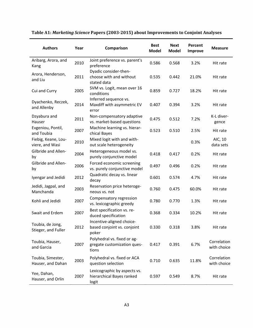
In Table A1, we list the authors, the year, and the predictive ability measures, if provided, for the

best method and the next to best method. When predictive abilities are reported for multiple condi-

tions, we average over conditions. Hit rate is the most-common metric, but some papers report other

metrics. In Table A1 there are examples of large increases in predictive ability—increases clearly large

enough to affect strategic differences, and there are examples of small increases—an indication that the

field cares about even small improvements. In addition to the papers listed in Table A1, Marketing Sci-

ence has published papers that address the efficiency of the experimental design (Liu and Arora 2011;

Toubia and Hauser 2007; Yu, Goos, and Vandebroek 2009), potential endogeneity (Hauser and Toubia

2005; Liu, Otter, and Allenby 2007), market share constraints (Gilbride, Lenk, and Brazell 2008), and

contingent value methods (Park and MacLachlan 2008).

We identified twenty-four conjoint-analysis-related papers published in Marketing Science be-

tween 2003 and 2015. Of these, seventeen reported increases in predictive ability. The median was

4.7%, the mean was 9.6%, the minimum was 0.2%, and the maximum was 60%. More than half (52.9%)

reported increases of less than five percent and 17.6% reported increases of less than one percent.

A3

Table A1: Marketing Science Papers (2003-2015) about Improvements to Conjoint Analyses

Authors Year Comparison Best Model

Next Model

Percent Improve Measure

Aribarg, Arora, and Kang 2010 Joint preference vs. parent's

preference 0.586 0.568 3.2% Hit rate

Arora, Henderson, and Liu 2011

Dyadic consider-then-choose with and without stated data

0.535 0.442 21.0% Hit rate

Cui and Curry 2005 SVM vs. Logit, mean over 16 conditions 0.859 0.727 18.2% Hit rate

Dyachenko, Reczek, and Allenby 2014

Inferred sequence vs. Maxdiff with asymmetric EV error

0.407 0.394 3.2% Hit rate

Dzyabura and Hauser 2011 Non-compensatory adaptive

vs. market-based questions 0.475 0.512 7.2% K-L diver-gence

Evgeniou, Pontil, and Toubia 2007 Machine learning vs. hierar-

chical Bayes 0.523 0.510 2.5% Hit rate

Fiebig, Keane, Lou-viere, and Wasi 2010 Mixed logit with and with-

out scale heterogeneity 0.3% AIC, 10 data sets

Gilbride and Allen-by 2004 Heterogeneous model vs.

purely conjunctive model 0.418 0.417 0.2% Hit rate

Gilbride and Allen-by 2006 Forced economic screening

vs. purely conjunctive model 0.497 0.496 0.2% Hit rate

Iyengar and Jedidi 2012 Quadratic decay vs. linear decay 0.601 0.574 4.7% Hit rate

Jedidi, Jagpal, and Manchanda 2003 Reservation price heteroge-

neous vs. not 0.760 0.475 60.0% Hit rate

Kohli and Jedidi 2007 Compensatory regression vs. lexicographic greedy 0.780 0.770 1.3% Hit rate

Swait and Erdem 2007 Best specification vs. re-duced specification 0.368 0.334 10.2% Hit rate

Toubia, de Jong, Stieger, and Fuller 2012

Incentive-aligned choice-based conjoint vs. conjoint poker

0.330 0.318 3.8% Hit rate

Toubia, Hauser, and Garcia 2007

Polyhedral vs. fixed or ag-gregate customization ques-tions

0.417 0.391 6.7% Correlation with choice

Toubia, Simester, Hauser, and Dahan 2003 Polyhedral vs. fixed or ACA

question selection 0.710 0.635 11.8% Correlation with choice

Yee, Dahan, Hauser, and Orlin 2007

Lexicographic by aspects vs. hierarchical Bayes ranked logit

0.597 0.549 8.7% Hit rate

A4

Appendix 3. Proofs to Results and Propositions (provided for review; to be available online)

Result 1. For → 0, ∗ > ∗ , ∗ > ∗ , and ∗ > ∗ . (Results in this appendix are stated in notational shorthand, but are the same as those in the text.)

Proof. This proof addresses first-order conditions. We address second-order and cross-partial conditions when we examine existence and uniqueness later in this appendix. As → 0, the logit curve becomes extremely flat, which motivates a Taylor’s Series expansion of market share around = ℓ. When = ℓ the logit equations for the market shares are identical for Firm 1 and 2, identical for all strate-gies, , , , , and symmetric with respect to Firm 1 and Firm 2. Thus, at = ℓ we have ∗ = ∗ = ∗ = ∗ = = ℓ

∗ = ∗ = ∗ = ∗ = = ℓ ∗ = ∗ = ∗ = ∗ = = ℓ

Because the prices and shares are identical, we have:

∗ = ∗ = ∗ = ∗ = 11 − = ℓ

Where the last step comes from substituting the equalities for in Equation 4b from the text, and sim-plifying using + = 1. We obtain the optimal price by solving the following fixed-point problem in : = 11 − = 2 ++ = 2 +

Because the right-hand side is decreasing in on the range [1, 1.5] there will be exactly one solution in the range of ∈ [1, 1.5] for small . We compute the partial derivatives of the ’s at = ℓ: = (1 − 2 ) ≡ γΔ , = 0 ≡ γΔ

= − ≡ γΔ , = (1 − ) ≡ γΔ , Δ = − ℓ

We now use a Taylor’s series expansion with respect to recognizing that higher order terms are ( ) or higher and, hence, vanish as → 0. Substituting the expressions for the partial derivatives into the first-order conditions (Equation 4b), multiplying by , and using the above notation, we obtain:

∗ = [ ( + Δ Δ) + ( + Δ Δ] + ( )( + Δ Δ) (1 − ) − Δ Δ + ( + Δ Δ) (1 − ) − Δ Δ + ( ) ∗ = + 2 Δ( Δ + Δ ) + ( )(1 − ) + Δ(1 − 2 )( Δ + Δ ) + ( )

Similarly,

A5

∗ = + 2 Δ( Δ + Δ ) + ( )(1 − ) + Δ(1 − 2 )( Δ + Δ ) + ( ) Because all terms in the numerators and denominators of ∗ and ∗ are clearly positive, we show that ∗ > ∗ for → 0 if: + 2 Δ( Δ + Δ )[ (1 − ) + Δ(1 − 2 )( Δ + Δ )]> + 2 Δ( Δ + Δ )[ (1 − ) + Δ(1 − 2 )( Δ + Δ )] After simplification and ignoring terms that are ( ), this expression reduces to: Δ [( Δ + Δ ) − ( Δ + Δ )][2 − 3 + 2 ] > 0

We need only show that both terms in brackets are positive. We show the first term in brackets is posi-tive because: ( Δ + Δ ) − ( Δ + Δ ) = ( (1 − ) − ) − ( (1 − ) − ) > 0

The last step follows from > . We show the second term is positive because its minimum occurs at = and its value at this minimum is 2 − 3 + 2 = . Thus, 2 − 3 + 2 is positive for all ∈ [0,1]. To prove that ∗ > ∗ for → 0 we use another Taylor’s series expansion and simplify by the same procedures. Most of the algebra is the same until we come down to the following term in brackets (now reversed because is more profitable for Firm 1 than as → 0). Taking derivatives gives:

= (1 − 2 ) ≡ γΔ = 0 ≡ γΔ

= (1 − ) ≡ γΔ = − ≡ γΔ

The corresponding expression in brackets becomes (for ∗ − ∗ ): ( Δ + Δ ) − ( Δ + Δ ) = ( (1 − ) − ) − ( (1 − ) − ) > 0

where the last step is true because > .

By exploiting symmetry, we have ∗ = ∗ , yielding the result that ∗ > ∗ = ∗ > ∗ .

Lemma 1. ∗ < (1 − ∗ ) and ∗ < (1 − ∗ ) . Related conditions hold for , ,and .

Proof. We use the first-order conditions (for ) as illustrated in Equation 4a. All terms are positive, so we cross multiply. The first expression holds if ∗ (1 − ∗ ) + ∗ (1 − ∗ ) > ∗ (1 −∗ ) + ∗ (1 − ∗ ), which is true if ∗ > ∗ . The latter holds whenever > ℓ for all by substituting directly into the logit equation. We prove the second expression by using the first-order conditions for ∗ . Related expressions hold for other positionings. For example, for the positions, ∗ < (1 − ∗ ) and ∗ < (1 − ∗ ) .

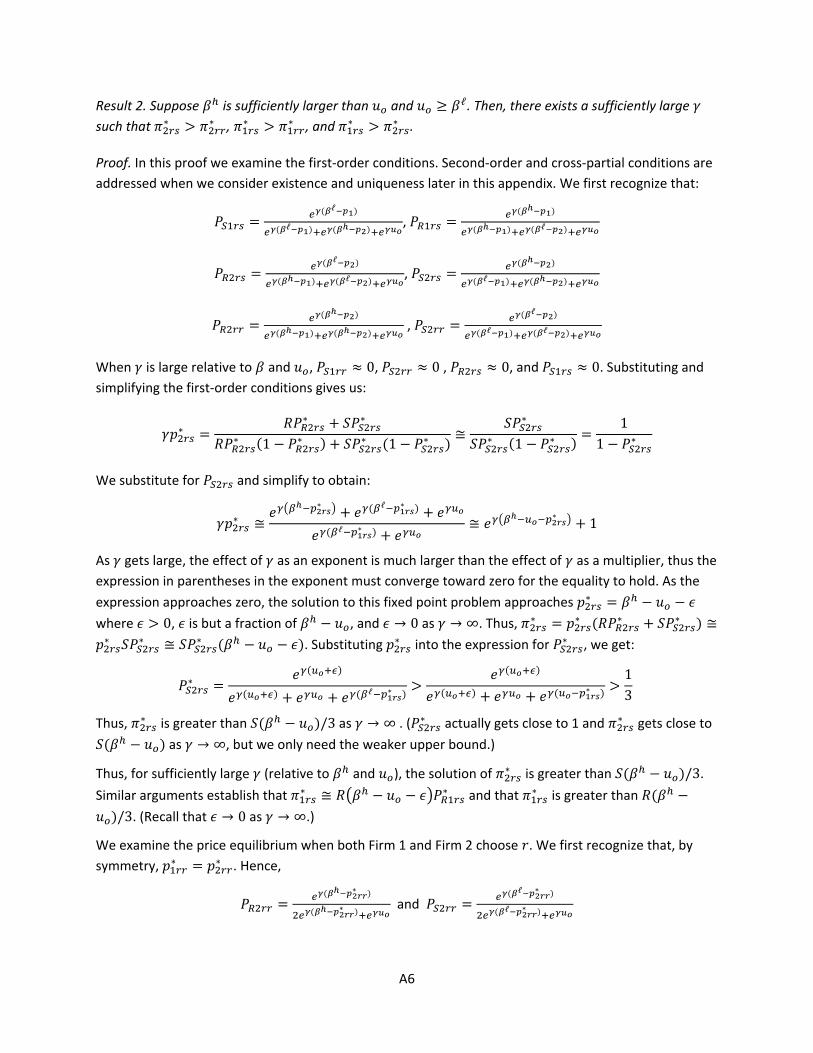
A6

Result 2. Suppose is sufficiently larger than and ≥ ℓ. Then, there exists a sufficiently large such that ∗ > ∗ , ∗ > ∗ , and ∗ > ∗ .

Proof. In this proof we examine the first-order conditions. Second-order and cross-partial conditions are addressed when we consider existence and uniqueness later in this appendix. We first recognize that: = ( ℓ )( ℓ ) ( ) , = ( )( ) ( ℓ )

= ( ℓ )( ) ( ℓ ) , = ( )( ℓ ) ( )

= ( )( ) ( ) , = ( ℓ )( ℓ ) ( ℓ )

When is large relative to and , ≈ 0, ≈ 0 , ≈ 0, and ≈ 0. Substituting and simplifying the first-order conditions gives us:

∗ = ∗ + ∗∗ (1 − ∗ ) + ∗ (1 − ∗ ) ≅ ∗∗ (1 − ∗ ) = 11 − ∗

We substitute for and simplify to obtain:

∗ ≅ ∗ + ( ℓ ∗ ) +( ℓ ∗ ) + ≅ ∗ + 1

As gets large, the effect of as an exponent is much larger than the effect of as a multiplier, thus the expression in parentheses in the exponent must converge toward zero for the equality to hold. As the expression approaches zero, the solution to this fixed point problem approaches ∗ = − − where > 0, is but a fraction of − , and → 0 as → ∞. Thus, ∗ = ∗ ( ∗ + ∗ ) ≅∗ ∗ ≅ ∗ ( − − ). Substituting ∗ into the expression for ∗ , we get:

∗ = ( )( ) + + ( ℓ ∗ ) > ( )( ) + + ( ∗ ) > 13 Thus, ∗ is greater than ( − )/3 as → ∞ . ( ∗ actually gets close to 1 and ∗ gets close to ( − ) as → ∞, but we only need the weaker upper bound.)

Thus, for sufficiently large (relative to and ), the solution of ∗ is greater than ( − )/3. Similar arguments establish that ∗ ≅ − − ∗ and that ∗ is greater than ( −)/3. (Recall that → 0 as → ∞.)

We examine the price equilibrium when both Firm 1 and Firm 2 choose . We first recognize that, by symmetry, ∗ = ∗ . Hence, = ( ∗ )( ∗ ) and = ( ℓ ∗ )( ℓ ∗ )

A7

We seek to show that there is a ∗ , with the properties that ∗ ≪ − and ∗ < , which

satisfies the first-order conditions. In this case, as → ∞, ∗ ≅ . The first-order conditions become:

∗ = ∗ + ∗∗ (1 − ∗ ) + ∗ (1 − ∗ ) ≅ 12 + ∗14 + ∗ (1 − ∗ ) ≤ 12 +14 = 2 + 4 < 6

The third to last step, setting ∗ = 1 for the inequality, is possible because the fraction increases in ∗ to obtain its maximum at ∗ =1, as shown with simple calculus. Thus, if ∗ satisfies the first-

order conditions, then ∗ < 6/ . By implication, ∗ < + < < − < ∗ for

sufficiently large. (We use the condition that > by a sufficient amount.) We establish ∗ < ∗ by similar arguments recognizing that, by symmetry, ∗ = ∗ , and using the proven

result that ∗ is greater than ( − ) for sufficiently large .

Result 3. ∗ = ∗ > ∗ = ∗ .

Proof. We examine the equations for the segment-based market shares to recognize that ( ∗ , ∗ ) = ∗ ( ∗ , ∗ ) and ( ∗ , ∗ ) = ∗ ( ∗ , ∗ ), and ∗ ( ∗ , ∗ ) >∗ ( ∗ , ∗ ). Thus, ∗ = ( ∗ , ∗ ) ≥ ( ∗ , ∗ ) = ∗ [ ( ∗ , ∗ ) +( ∗ , ∗ )] = ∗ [ ∗ + ∗ ] > ∗ [ ∗ + ∗ ] = ∗ . The second inequality is by the principle of optimality. The last inequality uses > and ∗ > ∗ . The equalities, ∗ = ∗ and ∗ = ∗ , are by symmetry.

Result 4. Suppose is sufficiently larger than and ≥ ℓ. Then, there exists a sufficiently large such that ∗ > ∗ .

Proof. By symmetry, we recognize that ∗ = ∗ . In the proof to Result 2 we established that ∗ ≅ − ∗ and ∗ ≅ − ∗ because → 0 as → ∞. We also see that the fixed-point problems are identical for ∗ and ∗ , thus, as → ∞, ∗ ≅ ∗ , which implies that ∗ ≅ ∗ . Putting these relationships together implies that ∗ ≅ − ∗ >− ∗ ≅ − ∗ ≅ ∗ = ∗

Proposition 1. For → 0, the innovator targets and the follower targets .

Proposition 2. If is sufficiently larger than and if ≥ ℓ, then there exists a sufficiently large such that the innovator targets and the follower targets .

Proof. We prove the two propositions together. Result 1 establishes that ∗ > ∗ as → 0. Result 2 establishes that ∗ > ∗ when is sufficiently large Thus, if Firm 1 chooses , Firm 2 chooses as → 0 and chooses when gets sufficiently large.

To prove that Firm 1 always chooses , we first consider the case where → 0. If Firm 1 chooses , then Firm 2 chooses by Proposition 1. Suppose instead that Firm 1 chooses , then Firm 2 will choose .

A8

Firm 2 will choose in this case because, by Result 1, ∗ > ∗ and, by symmetry, ∗ = ∗ , hence ∗ > ∗ = ∗ . If Firm 2 would choose whenever Firm 1 chooses , Firm 1 would earn ∗ . But ∗ = ∗ by symmetry and ∗ < ∗ = ∗ by Result 1. Thus, Firm 1 earns more profits ( ∗ ) by choosing than the profits it would obtain ( ∗ ) by choosing .

We now consider the case where is sufficiently large. Suppose Firm 1 chooses , then Firm 2 will choose by Result 2. Firm 1 receives ∗ . Suppose instead that Firm 1 chooses , then Firm 2 will choose because ∗ = ∗ by symmetry and ∗ > ∗ = ∗ under the conditions of Result 2. Thus, if Firm 1 chooses it receives ∗ . Because ∗ > ∗ by Result 4, Firm 1 will choose . Existence and Uniqueness. The existence and uniqueness arguments require substantial algebra. To avoid an excessively long appendix, we provide the basic insight. Detailed calculations are available from the authors. The proofs to Results 1-4 rely on the first-order conditions, thus we must show that a solu-tion to the first-order conditions, if it exists, satisfies the second-order conditions. The second-order conditions are illustrated by Equation 5a. We repeat them here the positions. ∗ = − ∗ (1 − ∗ )[2 − ∗ (1 − 2 ∗ )] − ∗ (1 − ∗ )[2 − ∗ (1 − 2 ∗ )] We use Lemma 1 to substitute (1 − ∗ ) for ∗ . The former is a larger value, so if the conditions hold for the larger value, they hold for ∗ . Algebra simplifies the right-hand side of the second-order condition to − { ∗ (1 − ∗ ) + ∗ (1 − ∗ )(1 − 2 ∗ + 2 ∗ )}. With direct substitu-tion in the logit model, recognizing ∗ ≥ ∗ , we show ∗ ≥ ∗ ≥ ∗ ≥ ∗ . (We show ∗ ≥ ∗ with implicit differentiation of the first-order conditions with respect to .) These inequali-ties imply that ∗ < min{ ∗ , 1 − ∗ }. Hence, ∗ (1 − ∗ ) ≥ ∗ (1 − ∗ ) whenever > . Thus, the second-order condition is more negative than − ∗ (1 − ∗ )(2 − 2 ∗ +2 ∗ ) < 0. We repeat the analysis for ∗ using a sufficient technical condition that either ∗ ≤ or

that the ratio of / is above a minimum value. (The condition, not shown here, requires only > 0 as → ∞.) Although our proof formally imposes the technical sufficient condition, we have not found any violation of the second-order conditions at equilibrium, even with small . Thus, with a (possible) mild restriction on , the second-order conditions are satisfied whenever the first-order conditions hold.

We now establish that the second-order conditions are satisfied on a compact set. We begin by showing algebraically that (1 − ∗ ) is decreasing in and that it decreases from a finite positive value, which we call ( = 0) > 1. As → ∞, (1 − ∗ ) decreases to 1. But increases from 0 to ∞, thus there must be a solution to = (1 − ) for every . Call this solution ( ). Because (1 − ∗ ) is decreasing in , it must be true that ≤ (1 − ) for all ∈ [0, ( )]. Using similar arguments we show there exists a ( ) such that ≤ (1 − ) for all ∈ [0, ( )]. Together ∈ [0, ( )] and ∈[0, ( )] define a compact set that is a subset of ∈ [0, (0)] and ∈ [0, (0)]. ( ( )is continuous and decreasing in and ( )is continuous and decreasing in ; ( ), ( ) > 0.) We have already established that ∗ ≥ ∗ ≥ ∗ ≥ ∗ when ∗ ≥ ∗ If we restrict the compact set to ≥ and the price difference is not too large, we

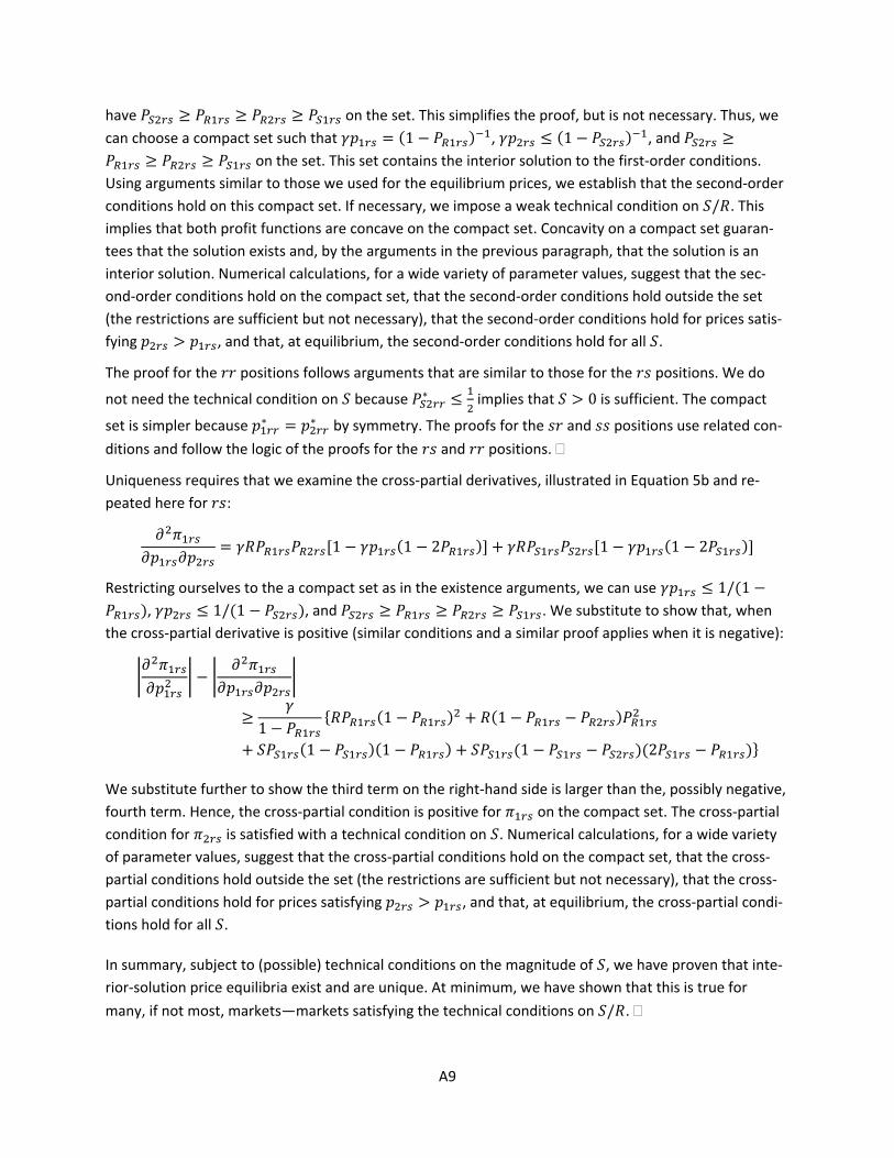
A9

have ≥ ≥ ≥ on the set. This simplifies the proof, but is not necessary. Thus, we can choose a compact set such that = (1 − ) , ≤ (1 − ) , and ≥≥ ≥ on the set. This set contains the interior solution to the first-order conditions. Using arguments similar to those we used for the equilibrium prices, we establish that the second-order conditions hold on this compact set. If necessary, we impose a weak technical condition on / . This implies that both profit functions are concave on the compact set. Concavity on a compact set guaran-tees that the solution exists and, by the arguments in the previous paragraph, that the solution is an interior solution. Numerical calculations, for a wide variety of parameter values, suggest that the sec-ond-order conditions hold on the compact set, that the second-order conditions hold outside the set (the restrictions are sufficient but not necessary), that the second-order conditions hold for prices satis-fying > , and that, at equilibrium, the second-order conditions hold for all .

The proof for the positions follows arguments that are similar to those for the positions. We do

not need the technical condition on because ∗ ≤ implies that > 0 is sufficient. The compact

set is simpler because ∗ = ∗ by symmetry. The proofs for the and positions use related con-ditions and follow the logic of the proofs for the and positions.

Uniqueness requires that we examine the cross-partial derivatives, illustrated in Equation 5b and re-peated here for : = [1 − (1 − 2 )] + [1 − (1 − 2 )] Restricting ourselves to the a compact set as in the existence arguments, we can use ≤ 1/(1 −), ≤ 1/(1 − ), and ≥ ≥ ≥ . We substitute to show that, when the cross-partial derivative is positive (similar conditions and a similar proof applies when it is negative): − ≥ 1 − { (1 − ) + (1 − − )+ (1 − )(1 − ) + (1 − − )(2 − )} We substitute further to show the third term on the right-hand side is larger than the, possibly negative, fourth term. Hence, the cross-partial condition is positive for on the compact set. The cross-partial condition for is satisfied with a technical condition on . Numerical calculations, for a wide variety of parameter values, suggest that the cross-partial conditions hold on the compact set, that the cross-partial conditions hold outside the set (the restrictions are sufficient but not necessary), that the cross-partial conditions hold for prices satisfying > , and that, at equilibrium, the cross-partial condi-tions hold for all .

In summary, subject to (possible) technical conditions on the magnitude of , we have proven that inte-rior-solution price equilibria exist and are unique. At minimum, we have shown that this is true for many, if not most, markets—markets satisfying the technical conditions on / .