The Strategic Implications of Scale in Choice-Based

Conjoint Analysis

by

John R. Hauser

Felix Eggers

and

Matthew Selove

October 2017

John R. Hauser is the Kirin Professor of Marketing, MIT Sloan School of Management, Massachusetts Institute of Technology, E62-538, 77 Massachusetts Avenue, Cambridge, MA 02142, (617) 253-2929, hauser@mit.edu.

Felix Eggers is an Assistant Professor of Marketing and Fellow of the SOM Research School at the Faculty of Economics and Business, University of Groningen, Nettelbosje 2, 9747 AE Groningen, The Nether-lands. 31 50 363 7065, f.eggers@rug.nl.

Matthew Selove is an Associate Professor of Marketing at The George L. Argyros School of Business and Economics, Chapman University, Beckman Hall 303L, 1 University Drive, Orange, CA 92866, se-love@chapman.edu.

The Strategic Implications of Scale in Choice-Based

Conjoint Analysis

Abstract

Choice-based conjoint (CBC) studies have begun to rely on simulators to forecast equilibrium

prices for patent/copyright valuations and for strategic product positioning. While CBC research has long

focused on the accuracy of estimated relative tradeoffs among attribute levels, predicted equilibrium

prices and strategic positioning are surprisingly and dramatically dependent on the magnitude of the

partworths relative to the magnitude of the error term (scale). Although the impact of scale on the abil-

ity to estimate heterogeneous partworths is well-known, neither the literature nor current practice has

addressed the sensitivity of pricing and positioning to scale. This sensitivity is important because (esti-

mated) scale depends on seemingly innocuous market-research decisions such as whether attributes are

described by text or by pictures. We demonstrate the strategic implications of scale using a formal mod-

el in which heterogeneity is modeled explicitly. If a firm shirks on the quality of a CBC study and acts on

incorrectly observed scale, a follower, but not an innovator, can make costly strategic errors. We

demonstrate empirically that image quality and incentive alignment affect scale sufficiently to change

strategic decisions and can affect patent/copyright valuations by hundreds of millions of dollars.

Keywords: Conjoint analysis, market research, choice models

1

1. Scale Affects Patent/Copyright Valuations and Strategic Decisions

With an estimated 18,000 applications per year, conjoint analysis is one of the most-used quan-

titative market research methods (Orme 2014; Sawtooth Software 2015). Over 80% of these conjoint

applications are choice-based. Firms routinely use choice-based conjoint analysis (CBC) to identify pre-

ferred product attributes in the hopes of maximizing profit—for example, General Motors alone spends

10s of millions of dollars each year (Urban and Hauser 2004). CBC is increasingly used in litigation and

courts have awarded billion-dollar judgments for patent or copyright infringement based on CBC studies

(Cameron, Cragg, and McFadden 2013; McFadden 2014; Mintz 2012).

Research in CBC has long focused on the ability to estimate accurate tradeoffs among product

attribute levels. Improved question selection, improved estimation, and techniques such as incentive

alignment all enhance accuracy and lead to better managerial decisions. However, with the advance-

ment of CBC simulators and faster computers, researchers, especially in litigation, have begun to use

CBC studies to estimate price equilibria and the resulting equilibrium profits (e.g., Allenby et al. 2014).

This use of CBC raises a new concern because, as shown in this paper, the calculated price equilibria

depend critically on the relative error term, i.e., the magnitude of the partworths relative to the magni-

tude of the error—called “scale” in the CBC literature. (We define scale as inversely proportional to the

standard deviation of the error as in Louviere [1993], recognizing that some authors define scale as pro-

portional to the standard deviation of the error as in Train [2009, p. 40]).

The implications are significant. We show that patent/copyright valuations can differ by hun-

dreds of millions of dollars depending upon scale. We also show that scale affects strategic positioning

decisions even when holding heterogeneity and unobserved attributes constant—a different phenome-

non than that commonly analyzed in the strategic positioning literature. These implications of scale are

important to practice because (1) patent/copyright valuations and strategic decisions are based on the

scale observed in a market-research study, (2) observed scale depends upon market research decisions

2

such as the realism of images or incentive alignment, and (3) observed scale can be adjusted, although

relatively rarely done so in practice, to reflect how consumers will actually behave in the marketplace

(vs. holdout choices or the choice-experimental setting).

We combine formal analysis with empirical research. By varying incentive alignment and the

realism of the stimuli, we demonstrate that the quality of market research affects the parameters of the

formal model sufficiently to have a large impact. With a subsequent market-validation study, we also

show that patent/copyright valuations can be substantially different if the court bases valuations on

observed (“internal”) scale versus (“external”) scale as adjusted to market validation. Furthermore, firms

may make different strategic decisions depending upon the quality of the CBC study and whether or not

scale is adjusted to the market.

It is obvious that, if the scale parameter upon which the court or firm bases its decisions is dif-

ferent from the scale parameter upon which market-based equilibrium price is based, then a court or

firm might make errors in its decisions. However, neither the magnitude and direction of the errors, nor

the large effect of seemingly minor market-research craft such as realistic images and incentive align-

ment are obvious. We reviewed the conjoint-analysis papers in Marketing Science from the last 15 years

(2003-2017). Forty-six (46) papers addressed new estimation methods, new adaptive questioning meth-

ods, methods to motivate respondents, more efficient designs, non-compensatory methods, and other

improvements. Mostly, papers focused on the improved estimation of relative partworths or managerial

interpretations. Five of the papers address scale (or a related concept for non-CBC papers), and of those

five, three focus on more accurate estimation, one on brand credibility, and one on peer influence.

None discuss the strategic (price or positioning) implications of scale.

Most papers do not report whether stimuli are text-only, pictorial, or animated, but of those

that do, the vast majority are text-only. Interest in incentive alignment is growing. No papers discuss the

impact of either stimuli presentation or incentive alignment on scale observed for the estimation data.

3

2. Deriving Implications from CBC Studies

We begin with a short review of current CBC practice. We then describe the implications when

CBC studies are used to calculate price equilibria.

2.1. Typical Current Practice

In CBC, products (or services) are summarized by a set of levels of the attributes. For example, a

smartwatch might have a watch face (attribute) that is either round or rectangular (levels), be silver or

gold colored, and have a black or brown leather band. By varying the smartwatch attribute levels sys-

tematically within an experimental design, CBC estimates preferences for attribute levels, called “part-

worths,” which describe the differential value of the attribute levels. For example, one partworth might

represent the differential value of a rectangular watch face relative to a round watch face.

Applied practice focuses on estimating accurately the relative partworths. For example, if rec-

tangular and round watch faces are equally costly, but the partworth of a rectangular watch face is

greater than the partworth of a round watch face for most consumers, then a typical recommendation

would be to launch a product with a rectangular watch face. The relative partworths can also be used to

calculate willingness-to-pay by comparing them to the CBC price coefficient. For example, if a consum-

er’s differential value between a rectangular and a round watch face is higher than a $100 reduction in

the purchase price, firms typically infer that the consumer is willing-to-pay more than $100 for a rectan-

gular rather than a round watch face. (There are subtleties in this calculation due to the Bayesian nature

of most estimates, but this is the basic concept.)

These implications depend only on the (distribution of) relative partworths, not scale. If we

double all partworths, including the price coefficient, for every respondent, the relative partworths are

unchanged; product development practice would still recommend a rectangular watch face, and any

patent/copyright valuation relying on willingness-to-pay would be unchanged. Nonetheless, the accura-

cy with which the relative partworths can be estimated (and their interpretation) depends upon ac-

4

counting for heterogeneity in scale during estimation (e.g., Beck, Rose, and Hensher 1993; Fiebig, et al.

2010; Pancreas, Wang, and Dey 2016; Swait and Louviere 1993). Scale heterogeneity affects partworth

estimation and comparisons and/or aggregation of respondents’ willingness to pay (WTP), but, once

those are accounted for, WTP does not depend upon a common (across respondent) increase or de-

crease in scale (e.g., Ofek and Srinivasan 2002, Eq. 15). The phenomenon we investigate is different from

scale heterogeneity; we focus on the strategic implications of scale assuming accurate relative part-

worths and assuming the estimation accounts for scale heterogeneity.

In practice, there are two methods to adjust scale in CBC simulations. One method adjusts scale

and partworths to match market shares and uses the adjusted scale and partworths in simulations (e.g.,

Gilbride, Lenk, and Brazell 2008). The adjustments are motivated by predictive ability rather than strate-

gic implications. The second method adjusts scale directly or in a procedure known as randomized first

choice (RFC) in which an additive error is included in the simulations. RFC automatically determines the

random perturbations to yield "approximately the same scale factor as the [logit] model" (Huber, Orme,

Miller 1999). Scale adjustments are easy to implement in the dominant simulation packages, but usage

is reported as rare—users almost always stick with the scale observed in the CBC estimation (Orme

2017). While some use the estimation scale by default, many users report that market data, as a

benchmark to adjust scale, are not available or not relevant to the simulated markets. Our formal model

and empirical illustration suggest that adjustments are critical and should be used much more often

than they are currently. We also provide an alternative adjustment that does not require market data.

2.2. Current Practice is Changing: The Implications of Price Equilibria

One method to calculate damages in patent/copyright cases is based on the additional profits

obtained due to the infringing level of an attribute. Because CBC studies have influenced billion-dollar

judgments (Mintz 2012), the state-of-the-art in CBC simulators is advancing rapidly. Due to the influence

of game theory in marketing science, CBC simulators are beginning to consider competitive response.

5

For example, if an innovator introduces a rectangular watch face and a follower responds with a round

watch face (and all other attributes are held constant), then CBC simulations can be used to calculate

the Nash price equilibrium. Based on equilibrium prices, simulators can calculate the follower’s most-

profitable response (rectangular vs. round) to the innovator’s new product. Allenby, et al. (2014) pro-

pose that damages be calculated as the equilibrium profits obtained with the patent/copyright in-

fringement minus the equilibrium profits that would have been obtained without the infringement.

Courts recognized the issue as early as 2005 for class-action cases (e.g., Whyte 2005, albeit not CBC) and

the use of CBC studies to calculate market-price equilibria are now debated in many high-profile pa-

tent/copyright case (and in many other types of litigation cases).

Although Sawtooth Software estimates 80% of managerial CBC applications consider competi-

tion in market simulations, less than 5% of CBC applications now use “game theory stuff” (Orme 2017).

Considering competitive reactions can lead to different implications than static simulations. We show

that scale plays a central role when calculating price equilibria and predicting optimal competitive reac-

tions.

2.3. Interpretation and Implications of the Error Term

The error term in CBC has many interpretations and implications. It has been interpreted as in-

herent stochasticity in consumer choice behavior and/or sources that are unobservable to the research-

er, such as unobserved heterogeneity, unobserved attributes, functional misspecifications, or consumer

stochasticity that is introduced by the CBC experiment (e.g., due to fatigue; e.g., Manski 1977; Thurstone

1927). We are most interested in what happens to the (observed) relative magnitude of the error term,

and consequently scale, when the quality of the CBC study changes, say by the addition of more-realistic

images or incentive alignment. To address this issue, we assume that the firm acts strategically on a CBC

study anticipating the implied price equilibria. However, after the firm selects its positioning strategy

(say a silver vs. gold smartwatch) and launches its product, the prices are set by market forces. Because

6

actual sales depend on how consumers react to the product’s attributes and price in the market place,

we need the concept of a “true” scale that represents how the market reacts. We purposefully do not

define “true” scale as a philosophical construct—it is defined as the scale that best represents how con-

sumers actually react in the marketplace. Practically, we expect the “true” scale to be finite because of

inherent stochasticity (e.g., Bass 1974), but the theory allows “true” scale to be finite or to approach

infinity.

Our formal model differs from prior models in the positioning literature because we explicitly

model heterogeneity in all partworths that are relevant to positioning decisions. In other words, in our

formal model we assume that the error term (in estimation) captures imperfections in the CBC study (if

any) plus any residual uncertainty. We explicitly assume the firms do not act on attributes that are un-

observed or on heterogeneity in consumer preferences that will be revealed when consumers purchase

the products. For “true” scale, the error term is limited to residual uncertainty (if any). With explicit het-

erogeneity we seek to rule out explanations that the firms act strategically upon heterogeneity as in de

Palma, et al. (1985, p. 780) who state: “the world is pervasively heterogeneous, and we have made it

clear how, in a particular model, this restores smoothness [that leads to differentiation].” Explicit heter-

ogeneity greatly complicates the proofs, but, we hope, provides new practical insight for the use of CBC

studies to calculate and act on price equilibria.

2.4. Research Philosophy

We use complementary formal models and empirical CBC studies to explore the impact of scale.

Each helps the other. The formal models illustrate that the observed empirical effects are based on

more-general concepts. The empirical studies show that the parameters of the formal model can be

estimated and that the predicted phenomena have real-world implications. Empirically, we vary two

aspects of the quality of CBC studies—realism of images and incentive alignment. Each of the aspects is

important by itself, but the two aspects are chosen to be illustrative of the larger issue. The method we

7

use to adjust scale illustrates that adjustments affect strategic decisions. We do not claim these are the

only feasible adjustments, although they are practical even when market data is unavailable.

3. Related Literature

3.1. Asymmetric Competition: Minimum versus Maximum Differentiation

The study of minimum versus maximum differentiation has a rich history in both economics and

marketing. Hotelling (1929) proposed a model of minimum differentiation in which consumers are uni-

formly distributed along a line and two firms compete by first choosing a position (attribute level) and

then a price. After demonstrating that the price equilibrium did not exist in Hotelling’s model,

d’Aspremont, Gabszewicz, and Thisse (1979) proposed quadratic transport costs and obtained an equi-

librium of maximum differentiation—firms choose strategic positions at opposite ends of the line. de

Palma, et al. (1985) and Rhee, et al. (1992) restored minimum differentiation to Hotelling’s line with

uncertainty about heterogeneity in preferences (partworth heterogeneity in our model). In their model,

each consumer’s utility depends on the transport cost from the firm to the consumer’s position on the

line and on an error-like term reflecting the firm’s uncertainty about the heterogeneity in consumer’s

tastes (and other attributes the consumer may value). Aggregate demand is given by a logit-like func-

tion. When the unknown heterogeneity is sufficiently large, the firm’s predictions are imprecise leading

to reduced price competition and minimum differentiation. We note that their “error” term captures

unobserved heterogeneity in consumer preferences rather than any stochasticity that remains after

heterogeneity and missing attributes are fully modeled. We extend their model to model heterogeneity

explicitly in order to study the practical implications of market research quality. In our formal model, we

are careful to rule out heterogeneity and strategic firm behavior with respect to unobserved attributes.

Many other researchers explore Hotelling-like models to derive conditions when differentiation

is likely and when it is not (e.g., Eaton and Lipsey 1975; Eaton and Wooders 1985; Economides 1984;

Graitson 1982; Johnson and Myatt 2006; Novshek 1980; Sajeesh and Raju 2010; Shaked and Sutton

8

1982; Shilony 1981). In these formal models, differentiation is driven by the heterogeneity of consumer

preferences—something we hold constant.

In marketing, Thomadsen (2007) shows how asymmetries in attribute levels lead one firm to

favor maximum differentiation in physical location while another favors minimum differentiation. Gal-or

and Dukes (2003) show that a two-sided market (commercial media serving consumers and advertisers)

reverses the differentiation found in d’Aspremont, Gabszewicz, and Thisse (1979). Guo (2006) extends

attribute-based analysis to forward looking consumers who observe one of two product attributes. Con-

sumers anticipate probabilistically future valuations for the other product attribute. In these models

heterogeneity in preferences (partworths) drives strategic behavior with respect to prices and profits.

In the language of CBC, all of these papers focus on the distribution of relative partworths or on

the partworths of unobserved or uncertain attributes. Although many models include error terms, none

analyze the effect of imperfect market research or inherent stochasticity. We show that these phenom-

ena alone can drive firm’s decisions on differentiation. The scale-based strategic analysis is a means to

an end. It gives us the machinery to understand the impact of the quality of CBC studies on forecast

equilibrium prices and on strategic decisions.

3.2. Price Equilibria in Heterogeneous Logit Models (as in CBC)

When there is no heterogeneity in partworths, Choi, DeSarbo and Harker (1990) demonstrate

that price equilibria exist if consumers are not overly price-sensitive. Their condition (p. 179) suggests

that price equilibria are more likely to exist if there is greater uncertainty in consumer preferences—a

result consistent with our model which, in addition, accounts for heterogeneity. Choi and DeSarbo

(1994) use similar concepts to solve a positioning problem with exhaustive enumeration. Luo, Kannan

and Ratchford (2007) extend the analysis to include heterogeneous partworths and equilibria at the

retail level. They use numeric methods to find Stackelberg equilibria if and when they exist.

State-of-the-art applications of CBC explicitly model consumer heterogeneity. Hierarchical Bayes

9

(HB) methods are most common, but latent structure, empirical Bayes, machine learning, and polyhe-

dral methods are also used (Andrews, Ansari, and Currim 2002; Evgeniou, Pontil, and Toubia 2007; Rossi

and Allenby 2003; Toubia, Hauser, and Garcia 2007). If we are to examine price equilibria using CBC, we

need to know that price equilibria exist and are unique. Unfortunately, Aksoy-Pierson, Allon, and Feder-

gruen (APAF, 2013) warn that price equilibria in heterogeneous logit models may not exist. APAF gener-

alize the analyses of Caplin and Nalebuff (1991) to establish sufficient conditions for price equilibria to

exist, to be unique, and to be given by the first-order conditions. The APAF conditions apply to typical

HB CBC studies (APAF, §6). Because of this warning, we address whether the equilibria exist and are

unique in our formal model and we check existence in our empirical analyses.

3.3. Improvements in CBC Methods are Common in the Literature

Many of the forty-six Marketing Science articles that we reviewed (see §1) focused on improved

estimation with a common focus on the accuracy with which partworths are estimated. Sawtooth Soft-

ware (2016) reports that many of these methods have been adopted by industry. Our paper explores

why the accurate estimation of scale matters for patent/copyright valuations and for managerial deci-

sions and, hence, provides an additional dimension and justification for improved methods. Our paper

on price/profit equilibrium considerations complements the academic and industry focus on the appro-

priate modeling of scale to improve relative partworth estimation and accurate predictive ability.

4. General Formulation and Basic Notation

We begin with the more-general model of consumer preference that we use for the empirical

studies in §9. Appendix 1 summarizes notation for both the general and stylized formal models. We

focus on a single attribute with two levels. Other attribute levels are common among products in the

market and do not affect strategic decisions. This focus is sufficient to illustrate the impact of scale and

is consistent with Irmen and Thisse (1998, p. 78), who analyze markets in which firms compete on multi-

ple dimensions and conclude that “differentiation in a single dimension is sufficient to relax price com-

10

petition and to permit firms to enjoy the advantages of a central location in all other characteristics.”

Our analysis also applies to simultaneous differentiation of a composite of multiple dimensions, say a

silver smartwatch with a rectangular face and a black leather band vs. a gold smartwatch with a round

watch face and a metal band.

To match typical applications of CBC, we focus on discrete (horizontal) levels of an attribute that

we label and . A product can have either or , but not both. If mnemonics help, think of as round,

regular, routine, ruby, or rust-colored and as square, small, special, sapphire, or scarlet. We focus on

two firms, each of which sells one product. We allow an “outside option” to capture other firms and

products that are exogenous to the strategic decisions of the two-firm duopoly.

Let be consumer ’s utility for Firm ’s product, let be ’s utility for the outside option,

and let be product ’s price. Let and be ’s partworths for attribute levels and , respectively,

and let and be indicator functions for whether or not Firm ’s product has or , respectively. Let

indicate ’s preference for price, let be an extreme value error term with variance /6 . If the

error terms are independent and identically distributed, we have the standard logit model for the prob-

ability, , that consumer purchases Firm ’s product (relative to Firm ’s product and the outside

option):

= + − +

= ( )( ) + ( , , ) +

To identify the model in estimation, we must set , , , or . For the remainder of the

theory development, we follow McFadden (2014), Sonnier, Ainslie, and Otter (2007), and Train (2003, p.

44) and parameterize the model so that the coefficient of price relative to or is unity. In particular,

we parameterize the logit model such that = 1. In this parameterization, the ’s are now relative

partworths and is scale. (We obtain the same theoretical and empirical implications with any parame-

11

terization in which scale is inversely proportional to the magnitude of the error term.) We focus on scale

in the theory development recognizing that, empirically, the quality of CBC studies can also affect the

accuracy with which the relative partworths are estimated. See §9.9. With our parameterization, the

CBC logit model for the formal analysis becomes:

(1) = ( )( ) + ( , , ) +

If is the market volume (including volume due to the outside option), is the marginal cost

for product , is Firm ’s fixed cost, and ( , , ) is the probability distribution over the relative

partworths and scale (posterior if Bayesian), then the profit, , for Firm is given by:

(2) = − ( , , ) −

(Empirically, if all estimates are Bayesian, we use the posterior distribution in the standard way.)

For the purposes of this paper, we assume that does not depend on the quantity sold nor the

choice of or . These assumptions can be relaxed and do not reverse the basic intuition in this paper.

(The effect of the relative cost of or is well-studied.)

5. Stylized Formal Model with Two-Segment Heterogeneity

To examine the strategic implications of scale while explicitly modeling heterogeneity, we focus

on two mutually exclusive and collectively exhaustive consumer segments. We label the segments R and

S, with segment sizes and , respectively. Partworths vary between segments, but are homogeneous

within segment ( = and = for all in segment R; = and = for all in seg-

ment S). Scale is constant across consumers such that = for all . The relative influence of a seg-

ment is captured by its size, or . This focus enables us to set = = and = = ℓ.

We set ≥ ℓ and ≥ without loss of generality so that consumers in Segment R prefer and con-

sumers in Segment S prefer and so that Segment R is at least as large as Segment S. Heterogeneity of

12

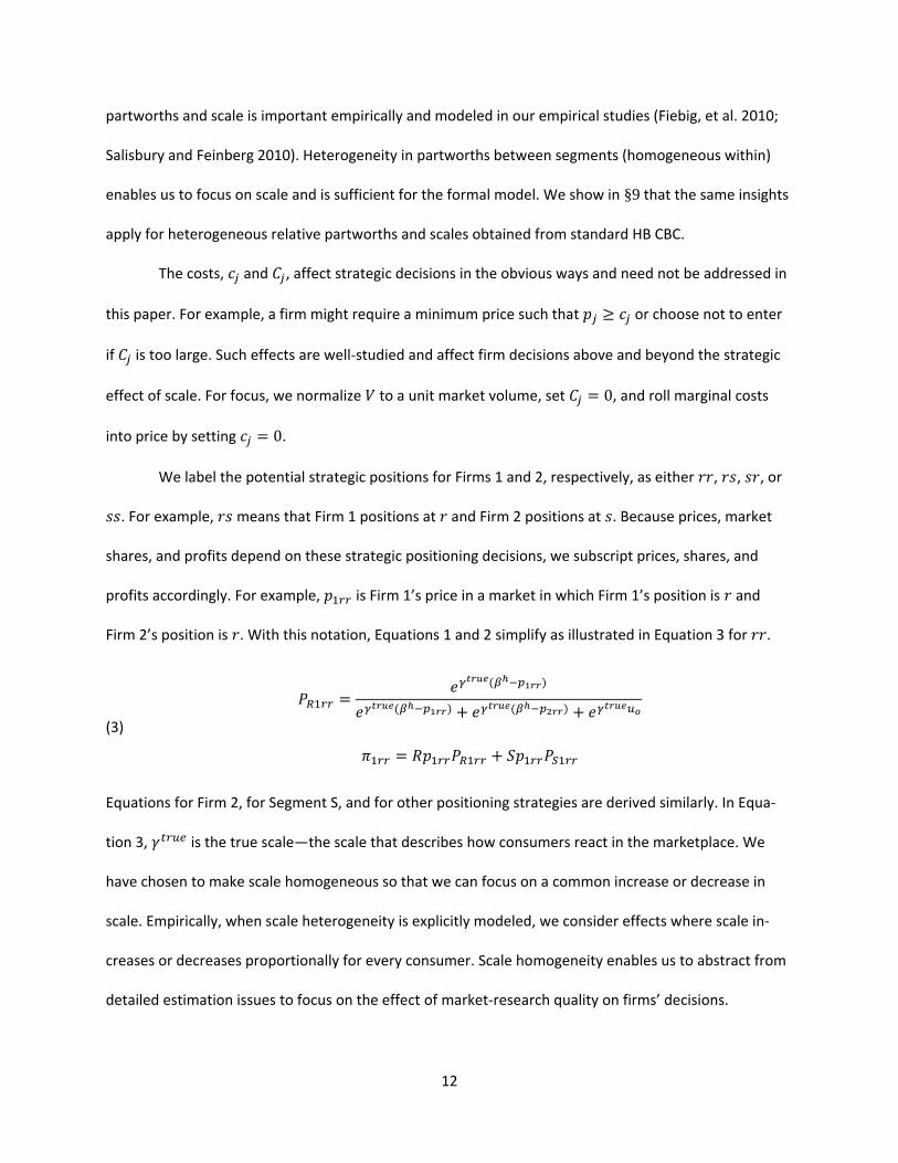
partworths and scale is important empirically and modeled in our empirical studies (Fiebig, et al. 2010;

Salisbury and Feinberg 2010). Heterogeneity in partworths between segments (homogeneous within)

enables us to focus on scale and is sufficient for the formal model. We show in §9 that the same insights

apply for heterogeneous relative partworths and scales obtained from standard HB CBC.

The costs, and , affect strategic decisions in the obvious ways and need not be addressed in

this paper. For example, a firm might require a minimum price such that ≥ or choose not to enter

if is too large. Such effects are well-studied and affect firm decisions above and beyond the strategic

effect of scale. For focus, we normalize to a unit market volume, set = 0, and roll marginal costs

into price by setting = 0.

We label the potential strategic positions for Firms 1 and 2, respectively, as either , , , or

. For example, means that Firm 1 positions at and Firm 2 positions at . Because prices, market

shares, and profits depend on these strategic positioning decisions, we subscript prices, shares, and

profits accordingly. For example, is Firm 1’s price in a market in which Firm 1’s position is and

Firm 2’s position is . With this notation, Equations 1 and 2 simplify as illustrated in Equation 3 for .

(3)

= ( )( ) + ( ) +

= +

Equations for Firm 2, for Segment S, and for other positioning strategies are derived similarly. In Equa-

tion 3, is the true scale—the scale that describes how consumers react in the marketplace. We

have chosen to make scale homogeneous so that we can focus on a common increase or decrease in

scale. Empirically, when scale heterogeneity is explicitly modeled, we consider effects where scale in-

creases or decreases proportionally for every consumer. Scale homogeneity enables us to abstract from

detailed estimation issues to focus on the effect of market-research quality on firms’ decisions.

13

5.1 Basic Game to Demonstrate the Impact of True Scale (Inherent Stochasticity)

The price-positioning game is consistent with key references in §3.1. Temporarily, we assume

the firms know , which may approach infinity. Based on this knowledge, the firms first choose their

product positions ( or ) sequentially, and then the market sets prices. The positioning decisions, once

made, are not easily reversible, perhaps due to production capabilities or ephemeral advertising invest-

ments. Without loss of generality, Firm 1 is the innovator and Firm 2 is the follower. The innovator en-

ters assuming that the follower will choose its positions optimally. (We abstracted away from entry deci-

sions by setting = = 0.) After the firms have entered, Nash equilibrium prices, if they exist, are

realized. If the firms know the true scale, they can anticipate these prices. (This two-stage game will be

embedded in another game in §7 in which firms do not observe the true scale.) We use * to indicate

Nash equilibrium prices, shares, and profits.

The equilibria we obtain, and strategies that are best for the innovator and follower, have the

flavor of models in the asymmetric competition literature (minimum vs. maximum differentiation), but

with two important differences. (1) Our results are not driven by unobserved heterogeneity or strategi-

cally-relevant unobserved attributes. (2) Our results are focused on providing a structure to understand

and evaluate the impact of improvements in CBC methods. The formal structure can be used as a practi-

cal tool to evaluate whether improvements, such as more-realistic images or incentive alignment, affect

strategic decisions.

Although we believe that, ex post, the qualitative effects are intuitive, they have not been dis-

cussed in the CBC literature. It is well known that scale affects logit-model-based market shares because

the logit curve is steeper in both attributes and price when scale increases, but we could find no discus-

sion of the implications of scale for price equilibria or strategic positioning. Papers which advocate the

use of estimated equilibrium prices do not discuss sensitivity to scale.

14

5.2 Equilibria in the Price Subgame

We begin with implicit first-order conditions for the realized prices recognizing that the market

will set prices based on the true scale.

= − ( )[ ( ) + ]( ) + ( ) + = − (1 − ) = + − { (1 − ) + (1 − )}

Using these relationships, we obtain implicit equations for the equilibrium prices and the corre-

sponding equilibrium profits. Similar equations apply for , , and and Firm 2:

(4a) ∗ = 1 ∗ + ∗∗ (1 − ∗ ) + ∗ (1 − ∗ )

(4b) ∗ = 1 ( ∗ + ∗ )∗ (1 − ∗ ) + ∗ (1 − ∗ ) Differentiating further, we obtain implicit second-order and cross-partial conditions (given in

Appendix 2, existence and uniqueness section). Using these conditions, we establish that interior equi-

libria exist and are unique given (mild) sufficient conditions. We test these conditions for our illustrative

examples and for our empirical analyses. In all cases, the equilibria in the illustrative example exist and

are unique. In our data, the empirical equilibrium exists for most posterior draws and, when they exist,

they are unique.

6. Sensitivity of Valuations and Strategic Decisions

In this section, we assume the firm knows the true scale and explore how scale affects pa-

tent/copyright valuations and strategic positioning decisions. In §7, we use these results to explore what

happens when decisions are based on observed scale rather than true scale.

6.1. Scale Affects the Price Equilibrium that are Calculated—Illustration

Consider the probability that a consumer in Segment R chooses the innovator’s product given

15

positions . By assumption, the relative partworths for vs. do not change, nor does the relative

preference for (or ) vs. price. However, the impact of these preference differences depends upon

. A larger makes more sensitive to both attribute differences and price differences; a

smaller makes less sensitive. As firms react to one another, a larger will drive the equi-

librium price downward.

As an illustration, we plot the equilibrium price of Firm 1 as a function of using the relative

partworths we obtained in our empirical study about smartwatches (details in §9). Figure 1 is based on a

CBC simulation with two firms whose products differ on watch-face color. We calculate the (counterfac-

tual) price equilibria for each level of . In Figure 1, the range of the scales is in the ranges reported

in the literature and in our empirical studies. The predicted equilibrium prices vary substantially.

Figure 1. Predicted Equilibrium Price Depends Upon the Scale of the CBC Study Used

to Calculate the Equilibrium Prices

Assume for this illustration that the smartwatch price swing in Figure 1 applies to smartphones.

(Smartphone prices are higher so that this will likely under-estimate the effect.) We can use publicly

available data to get an idea of the impact that scale would have had if equilibrium prices been used to

motivate damages in the first Apple v. Samsung trial about smartphone patents (Mintz 2012; willing-

$150

$170

$190

$210

$230

$250

$270

$290

$310

$330

$350

0.3 0.5 0.7 0.9 1.1 1.3

Inno

vato

r's E

quili

briu

m P

rice

True Scale

16

ness-to-pay, which is scale independent, was used in the 2012 trial). Using estimates of over 20 million

infringing Samsung smartphones (The Verge 2012), the calculated price swing of $100 implies a swing of

$2 billion in revenue. Patent/copyright valuations are based on profit differences, not revenue. Unfortu-

nately, margins are subject to “protective orders.” If the predicted multi-year profit due to the infringe-

ment were only a small fraction of the revenue swing implied by Figure 1, damages could easily vary by

tens of millions or even hundreds of millions of dollars depending upon the scale of the CBC analyses

used to calculate those damages. This swing is in the order of magnitude of the jury awards in the Apple

v. Samsung patent infringement cases (Mintz 2012).

6.2. True Scale Affects the Relative Profits of the Firms’ Positioning Strategies

To understand the effect of true scale on firms’ positioning strategies (choice of attribute levels

in equilibrium), we examine how profit-maximizing attribute levels change as true scale increases from

small to large. Because the functions are continuous, we need only show the extremes. Result 1 shows

that for sufficiently low true scale, price moderation through differentiation does not offset the ad-

vantage of targeting the larger segment. The proof is driven by the fact that the logit curve becomes

flatter as → 0. When price is endogenous, common intuition is not correct. All shares, including

the outside option, do not tend toward equality as → 0. The endogenous increase in equilibrium

prices offsets this effect. Instead, while the innovator and follower shares move closer to one another,

the equilibrium prices increase and reduce shares relative to the outside option. The proof demon-

strates that all of the countervailing forces balance to favor for the innovator and for the follower.

We provide details in Appendix 2.

Result 1. For sufficiently low true scale ( → 0), the follower prefers not to differentiate

whenever the innovator positions for the larger segment ( ∗ > ∗ ). However, the innovator

would prefer that the follower differentiate ( ∗ > ∗ ) and, if the follower were to differenti-

ate, the innovator would earn more profits than the follower ( ∗ > ∗ ).

17

We now show that the firms prefer different strategic positions if true scale is sufficiently high. It

is sufficient that (1) the relative partworth of is larger than the relative partworth of the outside option

and (2) the relative partworth of the outside option is at least as large as the relative partworth of .

With these conditions, market shares are sufficiently sensitive to price for large . Shares for differ-

entiated markets become more extreme, the equilibrium price is driven down, and shares increase rela-

tive to the outside option. The countervailing forces balance to favor for the follower.

Result 2. Suppose is sufficiently larger than and ≥ ℓ. Then, there exists a sufficiently

large such that the follower prefers to differentiate whenever the innovator positions for

the larger segment ( ∗ > ∗ ). Differentiation earns more profits for the innovator than no

differentiation ( ∗ > ∗ ), and those profits are larger than the profits earned by the follower

( ∗ > ∗ ).

Together Results 1 and 2 establish that, if the innovator targets the larger segment, then the fol-

lower will choose to differentiate ( ) when true scale is sufficiently high and will choose not to differen-

tiate ( ) when true scale is sufficiently low. All that remains is to show is that, in equilibrium, the innova-

tor will target the larger segment. While this may seem intuitive from Results 1 and 2, we need Results 3

and 4 to establish the formal result.

Result 3. Among the undifferentiated strategies, both the innovator and the follower prefer to

target the larger segment ( ∗ = ∗ > ∗ = ∗ ).

Result 4. Suppose is sufficiently larger than and > ℓ. Then, there exists a sufficiently

large such that the innovator prefers to differentiate by targeting the larger segment ra-

ther than the smaller segment ( ∗ > ∗ ).

6.3. Equilibrium in Product Positions

Results 1 to 4 establish necessary and sufficient conditions to prove the following propositions.

18

Proposition 1. For low true scale ( → 0), the innovator (Firm 1) targets the larger segment

( ) and the follower chooses not to differentiate. It also targets the larger segment ( ).

Proposition 2. If is sufficiently larger than and if ≥ ℓ, then there exists a sufficiently

large such that the innovator targets the larger segment ( ) and the follower chooses to

differentiate by targeting the smaller segment ( ).

Because the profit functions are continuous (see also APAF), Propositions 1 and 2 and the Mean

Value Theorem imply that there exists a such the follower is indifferent between and .

Numerically, for a wide variety of parameter values, the profit functions are smooth, the cutoff value is

unique, and ∗ − ∗ is monotonically increasing in . We have not found a counterexample.

We now have the machinery to address the issue of why scale is an important consideration

when CBC simulators are used for patent/copyright valuations and/or strategic decisions.

7. Implications for Investing in the Quality of CBC Studies

Higher “quality” in CBC can be expensive. Some firms, such as Procter & Gamble, Chrysler, or

General Motors are sophisticated and spend substantially on CBC. For example, some CBC studies invest

10s of thousands of dollars to create realistic animated descriptions of products and attributes complete

with training videos. Incentive alignment can also be expensive: one CBC study gave 1 in 20 respondents

$300 toward a smartphone and another gave every respondent $30 toward a streaming-music subscrip-

tion (Koh 2014; McFadden 2014). Firms routinely use high-quality Internet panels, often paying as much

as $5-10 for each respondent and up to $50-60 for hard-to-reach respondents. Our review of the litera-

ture (§1) suggests that firms believe that each of these investments increases the accuracy with which

relative partworths are estimated and eliminates sources that are not due to inherent stochasticity in

consumers’ choices. On the other hand, many firms reduce market research costs by using text-only

attribute descriptions, less-sophisticated methods, convenience samples, and small sample sizes. Many

“quality” decisions are driven by software defaults. We show that managerial implications are not trivial.

19

In §6, we temporarily assumed the firm knew the scale (defined as ) that described how

consumers would react to , , and price in the market. We are interested in what happens if the testify-

ing experts or firms shirk on their investments in the quality of CBC studies.

We embed the game from §6 into a larger game. We assume that if the firm invests more in the

CBC study, its estimate of scale becomes better, that is, − becomes smaller. To

focus on scale, we assume all (reasonable) CBC studies estimate the relative partworths correctly so that

the firm knows that > in R, > in S, and > . It is sufficient to illustrate the phenomenon if we

consider a lower-quality and a higher-quality CBC studies such that = in the higher-quality

study and ≠ in the lower-quality study. (In §9, we show that investments in more-realistic

images and incentive alignment lead to scale estimates that more accurately reflect how consumers in a

marketplace behave.) We seek to understand the implications of the firm’s decisions on market-

research quality. Thus,

1. The innovator decides whether to invest in the lower-quality or the higher-quality study.

(It needs at least the lower-quality study to determine > in R, > in S, and > .)

2. The innovator completes its CBC study and observes .

3. Based on its observed , the innovator announces and commits to either

or .

4. The follower decides whether to invest in the lower-quality or the higher-quality study.

(It needs at least the lower-quality study to determine > in R, > in S, and > .)

5. The follower completes its CBC study and observes . (The innovator’s

CBC study is private knowledge limited to the innovator.)

6. Based on its observed , the follower announces and commits to either

or .

7. Both firms launch their products. The market determines sales and price based on

20

—the scale that best describes consumer response. The firms realize their profits.

It will be obvious in §7.1 that the follower could have made its market research decision before

learning of the innovator’s positioning—either game ordering gives the same results. Commitment to

or implicitly assumes that positioning decisions are “sticky,” expensive, or based on know-how, pa-

tents, or copyrights. Once made, the firm cannot change its positioning even when the market price,

market shares, and profits are not as forecast. Propositions 1 and 2 give us sufficient insight to under-

stand the innovator’s and the follower’s market-research-quality decisions as they affect observed scale.

7.1 Innovator’s Strategic Positioning Decision Does Not Depend Upon Observed Scale

The innovator chooses to target the larger segment ( ) in both Propositions 1 and 2, thus the

innovator makes the same decision whether = or ≠ . Be-

cause the innovator’s strategic positioning decision is independent of the observed scale, investing in a

higher-quality CBC study has no effect on the innovator’s positioning strategy. (We state and prove the

result formally in Appendix 2.) The insight is consistent with recommendations in product development

(e.g., Urban and Hauser 1993, Ulrich and Eppinger 2004). These texts advise innovators to use market

research to identify the best attributes, but also advise that the accuracy need only be sufficient for a

GO/NO-GO decision.

7.2. Follower’s Strategic Positioning Decision Depends Upon Observed Scale

If a naïve follower underinvests in CBC studies, and if either < < or > > , then the follower makes a strategic error by choosing the wrong strategic

position (the wrong attribute level). (We state and prove the result formally in Appendix 2.) For exam-

ple, if < , then Proposition 1 implies that the most profitable attribute level for the follow-

er is . However, if the follower acts on = , and if < , then, by

Proposition 2, the follower will choose the less profitable attribute level, . In some cases, the naïve

follower may underinvest in CBC studies, but get lucky, say if < and < .

21

The first inequality implies is the follower’s most profitable attribute level and the second inequality

implies the follower chooses . The important insight is that, if the naïve follower underinvests in the

quality of a CBC study, then it is relying on luck to make the right decision. While it is often true that

getting a parameter wrong affects managerial decisions, it is somewhat surprising that simple design

decisions, such as whether or not to use text-only attributes, can have such a major effect.

Empirically, shirking on the quality of CBC market research can either increase or decrease ob-

served scale relative to true scale. For example, all else equal, we might expect that a text-based CBC

study would predict marketplace choices less precisely (lower scale) than a CBC study based on realistic

stimuli—the firm might underestimate (validation) scale with a text-based study. However, consumers

might answer text-based questions more consistently than realistic-stimuli-based questions. Scale as

observed in the estimation data might be high with text-based stimuli. Thus, if the firm calculates scale

using estimation data without adjusting scale for marketplace validation, it might overestimate scale. It

cannot know a priori whether the increase in observed scale due to the easier task counteracts the de-

crease in observed scale because the task represents the market less well. The amount by which ob-

served scale differs from true scale is an empirical question. (We provide empirical examples in §9.)

From a practical standpoint, if the cost of higher quality is small compared to the expected op-

portunity loss from making the wrong positioning decision, then the follower should invest in higher

quality CBC studies. §7.3 provides a formal method to make this decision.

7.3. Sophisticated Bayesian Follower’s Decision on Investments in CBC Studies

Sophisticated followers might anticipate that higher-quality CBC studies resolve their uncertain-

ty about true scale. Such sophisticated followers would make optimal decisions on whether or not to

invest in higher-quality CBC studies. Suppose that the follower has prior beliefs, ( ), about the

true scale and can pay dollars to resolve that uncertainty ( = ). (For simplicity of exposi-

tion, we normalize the cost of the lower-quality CBC study to zero.) Suppose further that the estimates

22

of the relative partworths are the same for both the higher- and lower-quality CBC studies, but only the

higher-quality study resolves . Because the follower knows the relative partworths and is sophisti-

cated, we assume the follower can calculate anticipated ∗ ( ) and ∗ ( ) for all values of

. The sophisticated follower must decide whether or not to invest dollars for higher quality.

If a sophisticated follower invests only in the lower-quality CBC study, it does not resolve ( ) and its expected profits are given by an expectation over ( ). The risk-neutral follower’s

expected profits with lower-quality research are:

(6) [ ∗( ℎ)]= ∗ ( ) ( ) , ∗ ( ) ( )

On the other hand, if the follower invests in a higher-quality CBC study, it resolves its estimate

of scale such that = . For each observed , the follower anticipates that it will choose

if ∗ ( ) < ∗ ( ), if ∗ ( ) > ∗ ( ), and choose randomly if ∗ ( ) =∗ ( ). Let Δ ( ) = 1 indicate that it is optimal for the follower to choose for an observed

and Δ ( ) = 0 indicate that it is optimal to choose after is revealed by higher-quality

market research. Then the risk neutral follower will use the maximum-profit-indicator function (Δ ) to

integrate over ( ). The expected profits when the sophisticated risk-neutral follower invests in

higher-quality market research are:

(7) [ ∗(ℎ ℎ ℎ)]= { ∗ ( )Δ ( ) + ∗ ( )[1 − Δ ( )]} ( ) −

To decide on whether or not to invest in the higher-quality CBC study, the sophisticated follower need

only compare the profits given by Equations 6 and 7. Because the notation in Equations 6 and 7 is cum-

bersome, we illustrate the comparison more simply and intuitively in §8 with an illustrative example.

23

In summary, the solution to the larger game is that the innovator never invests to resolve scale

( ). Lower-quality market research is sufficient as long as the CBC study reveals sufficiently accurate

relative partworths ( > in R, > in S, and > ). The sophisticated follower chooses whether to

invest by choosing the market research that maximizes profits comparing Equations 6 and 7). Naively

relying on the scale observed in a lower-quality CBC study might lead to substantial opportunity losses.

Unfortunately, our experience suggests that many firms make “gut” decisions on CBC investments and

choose aspects of CBC studies that we suspect are lower-quality. To the extend such firms are unaware

of the implications of scale on strategic decisions, such “gut” decisions may or may not be optimal.

The solution to the game cautions us about the use of price and profit equilibria in pa-

tent/copyright valuations. If the quality of the CBC is such that the testifying expert cannot assure the

court that ≅ , then the CBC simulation may not even model the correct position-

ing decision in a world without infringement (the “but-for” world). This caution is in addition to the cau-

tion from Figure 1 that an inaccurate estimate of scale can lead to a substantial error in the magnitude

of damages.

8. Illustrative Example, with Comments on Patent/Copyright Valuations

We illustrate the formal insights with a numerical example in which = 2, ℓ = 1, = 1,

and = 0.55. We obtain the fixed-point price equilibria by simple iteration combined with grid search.

In all cases, we check that the second-order and cross-partial conditions are satisfied. (R program availa-

ble from the authors.)

8.1. Representative Equilibria for Various Levels of Scale

Table 1 reports price equilibria for differentiated strategies ( ) for different values of scale

( ). In practice we expect to be the order of magnitude of the partworths, but to illustrate key

issues we vary over a wider range. For very small values of true scale ( = 0.05), the market is

less sensitive to price allowing firms to price highly and earn substantial profits. Profits and prices de-

24

crease with . For very large values of , the innovator’s share in segment S ( ∗ ) approaches

zero as does the follower’s share in Segment R ( ∗ ). The market becomes more segmented when true

scale increases.

Table 1. Prices, Shares, Profits, and Second-order Conditions: Differentiated Market

Scale Prices Shares in Segment R

Shares in Segment S Profits Second Order

Conditions

∗ ∗ ∗ ∗ ∗ ∗ ∗ ∗ ∗

∗

0.05 24.625 24.603 0.192 0.183 0.183 0.192 4.622 4.600 -0.009 -0.009 0.50 2.588 2.564 0.261 0.160 0.158 0.264 0.556 0.531 -0.103 -0.107 0.60 2.190 2.166 0.278 0.155 0.146 0.299 0.485 0.459 -0.132 -0.126 0.70 1.909 1.885 0.295 0.149 0.139 0.316 0.435 0.408 -0.157 -0.149 0.80 1.701 1.677 0.311 0.143 0.133 0.334 0.398 0.370 -0.184 -0.173 0.90 1.543 1.519 0.328 0.136 0.195 0.275 0.371 0.342 -0.212 -0.198 1.0 1.418 1.394 0.345 0.130 0.126 0.352 0.349 0.316 -0.137 -0.144 2.0 0.923 0.905 0.501 0.070 0.067 0.511 0.282 0.243 -0.491 -0.573 3.0 0.817 0.807 0.614 0.031 0.030 0.621 0.287 0.240 -0.808 -0.589 4.0 0.787 0.783 0.692 0.013 0.013 0.696 0.304 0.251 -1.200 -1.481 5.0 0.779 0.778 0.747 0.005 0.005 0.747 0.322 0.264 -1.639 -2.018 10 0.805 0.805 0.876 0.000 0.000 0.876 0.388 0.317 -3.938 -4.815 20 0.861 0.861 0.942 0.000 0.000 0.942 0.446 0.365 -8.477 -10.36

200 0.974 0.974 0.995 0.000 0.000 0.995 0.533 0.436 -89.54 -109.4

Table 2 reports equilibria for undifferentiated strategies ( ) using the same values of true scale

as in Table 1. The second-order conditions are always satisfied for undifferentiated strategies. Low true

scale implies high prices and profits. When true scale is large, the market is very sensitive to price and

the shares in Segment R approach 50%. If the firms do not differentiate, the high price sensitivity due to

large scale drives profits to zero. The last two columns of Table 2 compare profits between a differenti-

ated ( ) strategy and an undifferentiated strategy ( ). For low scale (below 1.0), strategy is more

profitable than for the follower. This is shown in a red bold font.

25

Table 2. Prices, Shares, Profits, and Relative Profits: Undifferentiated Market

Scale Prices Shares in Segment R

Shares in Segment S Profits Relative

Profits

∗ ∗ ∗ ∗ ∗ ∗ ∗ ∗ ∗ − ∗

∗ −∗ 0.05 24.619 24.619 0.190 0.190 0.184 0.184 4.618 4.618 0.004 -0.018 0.50 2.553 2.553 0.240 0.240 0.179 0.179 0.542 0.542 0.014 -0.011 0.60 2.147 2.147 0.251 0.251 0.178 0.178 0.468 0.468 0.017 -0.009 0.70 1.858 1.858 0.262 0.262 0.176 0.176 0.415 0.415 0.020 -0.007 0.80 1.642 1.642 0.272 0.272 0.175 0.175 0.375 0.375 0.023 -0.005 0.90 1.474 1.474 0.283 0.283 0.173 0.173 0.345 0.345 0.026 -0.002 1.0 1.341 1.341 0.294 0.294 0.172 0.172 0.320 0.320 0.029 0.004 2.0 0.744 0.744 0.385 0.385 0.156 0.156 0.209 0.209 0.072 0.034 3.0 0.539 0.539 0.444 0.444 0.142 0.142 0.166 0.166 0.121 0.074 4.0 0.425 0.425 0.476 0.476 0.134 0.134 0.137 0.137 0.167 0.114 5.0 0.349 0.349 0.491 0.491 0.130 0.130 0.114 0.114 0.208 0.150 10 0.177 0.177 0.500 0.500 0.127 0.127 0.059 0.059 0.329 0.258 20 0.089 0.089 0.500 0.500 0.127 0.127 0.029 0.029 0.416 0.335

200 0.009 0.009 0.500 0.500 0.127 0.127 0.003 0.003 0.530 0.433

8.2. Plot of Relative Profits as a Function of Scale

Figure 2 plots differentiated minus undifferentiated profit for values of true scale ( ) in the

range of [0, 2]. In Figure 2, the range of true scale is approximately equal to the values of the partworths

( ℓ and ). The innovator (black dashed line) always hopes that the follower will differentiate, but the

follower (red solid line) only chooses to differentiate when is approximately 1.0 or greater. In Fig-

ure 2, profit differences are smooth and monotonic; the critical value of is unique ( ≅ 1).

In §9 we provide a similar figure, but for empirical data.

26

Figure 2. Relative Profits of Differentiated vs. Undifferentiated Positioning Strategies

8.3. Illustration of an Optimal Decision on CBC-Based Market Research

Decisions on CBC-based market research spending depend upon Equations 6 and 7. Suppose, for

the sake of illustration, that the market potential is 10 million units and that prices are scaled in dollars.

Suppose further that the follower anticipates that the higher-quality CBC study reveals the true scale, = . It will act on the that is revealed. It uses its prior to anticipate the that will

be revealed. The lower-quality CBC study does not reveal , therefore the follower must act based

on its prior. If the follower chooses the lower-quality CBC study, the follower bases its positioning strat-

egy based on expected profits, integrating over ( ). The calculations are given in Table 3.

Based on Table 3, an undifferentiated strategy has a higher expected value than a differentiated

strategy, hence the follower using a lower-quality CBC study would choose as per Equation 6. If the

follower invests in the higher-quality CBC study, the follower can choose its strategy ( or ) depending

upon the it observes. The follower’s decision after observing is indicated by the “Best Strate-

gy” column. Choosing the best strategy for each realized yields higher expected profits

($5,034,722) compared to the best strategy based only on the lower-quality study ($4,981,407). The

difference, $53,315, is the most that a sophisticated follower would pay for a higher-quality CBC study.

-0.04

-0.02

0.00

0.02

0.04

0.06

0.08

0.1 0.2 0.3 0.4 0.5 0.6 0.7 0.8 0.9 1 1.1 1.2 1.3 1.4 1.5 1.6 1.7 1.8 1.9 2.0Prof

it di

ffere

ntia

ted

--Pr

ofit

undi

ffere

ntia

ted

True Scale

Innovator

Follower

27

Table 3. Illustration of the Follower’s Decisions and Outcomes Based on Either a Lower-

Quality CBC Study (Columns 3&4) or a Higher-Quality CBC Study (Column 6)

Prior, ( ) True Scale,

Follower Chooses Based on Lower-

Quality CBC Study

Follower Chooses Based on Lower-

Quality CBC Study

Best Strategy After Revealed

Follower Chooses or after Higher-

Quality CBC Study 0.03 0.1 $23,337,834 $23,509,998 r $23,509,998 0.03 0.2 $12,027,032 $12,186,344 r $12,186,344 0.08 0.3 $8,275,610 $8,420,431 r $8,420,431 0.08 0.4 $6,414,787 $6,543,437 r $6,543,437 0.08 0.5 $5,310,777 $5,421,558 r $5,421,558 0.08 0.6 $4,585,625 $4,676,841 r $4,676,841 0.08 0.7 $4,077,318 $4,147,275 r $4,147,275 0.08 0.8 $3,704,817 $3,751,862 r $3,751,862 0.08 0.9 $3,423,066 $3,445,561 r $3,445,561 0.08 1.0 $3,204,993 $3,201,369 s $3,204,993 0.03 1.1 $3,033,356 $3,002,089 s $3,033,356 0.03 1.2 $2,896,596 $2,836,255 s $2,896,596 0.03 1.3 $2,786,715 $2,695,922 s $2,786,715 0.03 1.4 $2,697,959 $2,575,425 s $2,697,959 0.03 1.5 $2,626,085 $2,470,611 s $2,626,085 0.03 1.6 $2,567,891 $2,378,368 s $2,567,891 0.03 1.7 $2,520,907 $2,296,323 s $2,520,907 0.03 1.8 $2,483,216 $2,222,635 s $2,483,216 0.03 1.9 $2,453,264 $2,155,856 s $2,453,264 0.03 2.0 $2,429,844 $2,094,834 s $2,429,844

Expected Profits $4,975,580 $4,981,407 $5,034,722

Table 3 also illustrates that a naïve follower can make strategic errors. Suppose the follower in-

vests in a lower-quality CBC study that tells the firm (incorrectly) that = 0.1. Believing and acting

on the lower-quality CBC study, the follower would choose not to differentiate ( ) and forecast a profit

of over $23.5M. If true scale were really = 2.0, then the firm would (1) position the product incor-

rectly ( rather than ), (2) bear an opportunity cost of $335,010, and (3) not realize anywhere near its

anticipated profit ($2.1M vs. $23.5M).

8.4. Implications for Patent and Copyright Valuations

Suppose the scale of a CBC study is and suppose that ≠ ,

28

then calculated prices and profits may either be too low or two high. Tables 1 and 2 suggest the differ-

ences can be quite large. Consider a patent valuation scenario in which is enabled by a patent and

represents the non-infringing alternative. Suppose the infringing firm competes in the market with a

firm that owns the patent and chooses a position, .

In this case, the proposed equilibrium-priced-based patent valuation would be the difference in

the infringing firm’s profits (the follower in our model) in an market versus the same firm in an

market. We use −( ∗ − ∗ ) from Table 2. For = 0.5, the valuation would be 0.011,

but for = 0.9, the valuation would be 0.002. Such differences in are

not unreasonable—we get at least a 2-to-1 swing in §9. But this difference implies an over five-fold dif-

ference in damages. (If = 0.05, damages would increase nine-fold.) Given that patent

valuations can be in the hundreds of millions of dollars or more, this is a huge difference. While our ex-

ample is based on a stylized formal model and the scales are purely illustrative, the example cautions

that scale and, by implication, the quality of the CBC study, is an important consideration for pa-

tent/copyright valuation. Interestingly, if ≥ 1, then the equilibrium profit calculations

imply that the infringing firm would have been better off by not infringing—an interesting interpretation

for the courts to consider. The effect is real—CBC studies used in litigation vary widely in the quality of

images, incentive alignment, and other aspects that might affect the (estimated) scale that is used in the

damages calculation.

9. Empirical Test: Smartwatches

We seek to influence CBC practice when price equilibria are used for patent/copyright valua-

tions and/or strategic positioning. In particular, we seek to determine whether the insights from the

stylized formal model and illustrative example translate to a real CBC study. To address practical rele-

vance, we address three empirical questions:

• Can we manipulate observed scale ( ) with more-realistic images and incentive

29

alignment (an illustration with two aspects of quality)?

• Can we obtain results analogous to those derived with the stylized formal model, but with het-

erogeneous partworths (and scales) from an HB CBC study using a representative panel of re-

spondents?

• Does it matter whether observed scale is based on estimated partworths or whether scale is ad-

justed based on a validation task that mimics the marketplace (an illustration of scale adjust-

ment)?

9.1. Higher- and Lower-Quality CBC Studies

We designed two CBC studies to match typical empirical practice. One study uses software de-

faults and mimics a lower-quality study, which is typical of many, but not all, CBC studies used for pa-

tent/copyright valuation. The other study used what is normally considered higher (and more costly)

quality by manipulating two aspects of quality, i.e., more-realistic images and incentive alignment. We

hold all other design variables constant between the two studies.1

The product category was smartwatches. We abstracted from the large number of attributes in

smartwatches to focus on case color (silver or gold), watch face (round or rectangular), watch band

(black leather, brown leather, or matching metal color), and price ($299 to $449). Following industry

practice, we held all other attributes constant, including brand and operating system, so that we could

estimate the relative tradeoffs among the attribute levels that we varied. Our focus on three smart-

watch attributes and price is sufficient to test the generalizability of the stylized model; an industry

study might vary more attributes. Empirically, any unobserved attributes do not vary between higher-

vs.-lower quality studies. By assumption for the worlds we simulate, unobserved attributes are not used

strategically for positioning decisions.

1 The two studies were part of a larger experimental design that also manipulated other aspects of quality in a fractional facto-rial design—for the purposes of this comparison those aspects were randomized. For brevity, we focus on the two most impact-ful aspects of quality. Details on the less impactful aspects are available from the authors.

30

We used sixteen choice sets for estimation (and two for internal validation) with three profiles

per choice set. We included the outside option via a dual-response procedure. These settings are typical

for current industry applications (Meissner, Oppewal, and Huber 2016; Wlömert and Eggers 2016). We

followed standard survey design principles including extensive pretesting (28 respondents in the higher-

quality study and 38 in the lower-quality study) to assure that (1) the questions, attributes, and tasks

were easy to understand and (2) that the manipulation of research quality between respondents was

not subject to demand artifacts.

9.2. Higher-Quality Study: Animations, Realistic Pictures, and Incentive Alignment

After the screening questions, respondents entered the CBC section. Respondents completed a

training task (not used in estimation), then saw an animated video to induce incentive alignment2 (e.g.,

Ding 2007; Ding, Grewal, and Liechty 2005; Ding, et al. 2011). Specifically, respondents were told that

some respondents (1 in 500) would receive a smartwatch and/or cash with a combined value of $500—

based on their answers to the survey. See Figure 3. Each respondent chose among realistic images of

three smartwatches and then indicated whether or not he or she would purchase the smartwatch (Fig-

ure 4). To make the images more realistic, the respondent could toggle among a detailed view, a top

view, and an app view (not shown in Figure 4). Dahan and Srinivasan (2000) suggest visual depictions

and animations provide nearly the same results as physical prototypes.

2 The incentive-alignment video is available at https://www.youtube.com/watch?v=DBLPfRJo2Ho.

31

Figure 3. Incentive Alignment Screenshot from the Higher-Quality Study

Figure 4. Higher-Quality Study: Choice-Based Dual Response Task (The images were animated allowing respondents to toggle views.)

9.3. Lower-Quality CBC Study: Text-based with No Incentive Alignment

In the lower-quality study, respondents also completed a training task but did not see the incen-

tive-alignment video, did not receive an incentive-alignment promise, saw only text-based stimuli (with

32

simple images), and could not toggle among views. See Figure 5. Respondents took part in a lottery for a

1 in 500 chance to win $500 in cash; however, the reward was not tied to the answers given in the low-

er-quality survey as it was in the higher-quality study.

Figure 5. Lower-Quality Study: Choice-Based Dual Response Task (no ability to toggle)

9.4. Validation Task to Estimate Scale Adjustments

We created a marketplace with twelve smartwatches and an outside option. (Twelve smart-

watches represents all possible design combinations.) Smartwatches varied on case color, watch face,

watch band, and price. Starting three weeks after the two CBC studies, respondents, in both the higher-

and lower-quality studies, were given an incentive-aligned opportunity to choose either one of the

twelve smartwatches or the outside option. We used the validation data to adjust the scale factor (§9.7).

Marketplace market shares were not available for these studies, but, in practice, researchers might con-

sider other validation adjustments such as those proposed by Gilbride, Lenk, and Brazell (2008).

9.5. Sample

Our sample was drawn from a professional panel.3 We screened the sample so that respondents

expressed interest in the category, were based in the US, aged 20-69, and agreed to informed consent

as required by our internal review boards. We also screened out respondents who already owned a

3 Peanut Labs is an international panel with 15 million pre-screened panelists from 36 countries. Their many corporate clients cumulatively gather data from approximately 450,000 completed surveys per month. Peanut Labs is a member of the ARF, CASRO, ESOMAR, and the MRA and has won many awards: web.peanutlabs.com.

33

smartwatch. Such screening is reasonable for our research purpose. Respondents in both studies re-

ceived standard panel incentives for participating in the study.

Overall, 858 respondents completed the first wave of studies: 427 in the higher-quality study,

431 in the lower-quality study. The rate of consumers who completed the validation study was equally

distributed (both 0.69). We only considered respondents in the analyses who completed the validation

study and removed respondents who always chose the outside option. There were no significant differ-

ences between the studies and the exclusion of respondents ( = 0.74). The final sample size was 545

(270 in the higher-quality study, 275 in the lower-quality study).

9.6. Estimation

We estimate a joint HB CBC model in which the relative partworths are drawn from the same

hyper-distribution, but scale ( ) varies between higher- and lower-quality and between estimation and

validation. We normalize a scale-adjustment to 1.0 for the lower-quality estimation sample so that

scale-adjustment for the other conditions can be identified. We assume a normal prior for the design

partworths and constrain the price coefficient by assuming a log-normal distribution (Allenby, et al.

2014). To avoid misspecification errors, we tested for interaction effects but could not detect significant

improvements in model fit; our model is based on main effects. The remaining settings followed stand-

ard procedures (Sawtooth Software 2015).

In the estimation, we used 10,000 burn-in iterations and a subsequent 10,000 iterations to draw

partworths, from which we kept every 10th draw. Based on these data, HB CBC provides a posterior dis-

tribution of relative partworths and estimated scales. All subsequent summaries, profits, and other re-

ported quantities are based on the posterior distributions.

9.7. CBC Quality Affects Observed Scale

Our first research question is whether the improvements in quality affects observed scale. The

posterior means and standard deviations of the scale-adjustment posterior distributions are given in

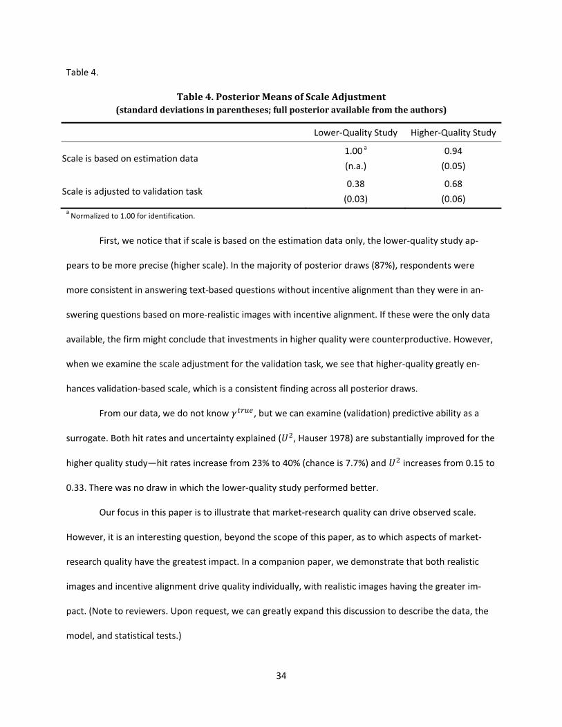
34

Table 4.

Table 4. Posterior Means of Scale Adjustment (standard deviations in parentheses; full posterior available from the authors)

Lower-Quality Study Higher-Quality Study

Scale is based on estimation data 1.00 a (n.a.)

0.94 (0.05)

Scale is adjusted to validation task 0.38 (0.03)

0.68 (0.06)

a Normalized to 1.00 for identification.

First, we notice that if scale is based on the estimation data only, the lower-quality study ap-

pears to be more precise (higher scale). In the majority of posterior draws (87%), respondents were

more consistent in answering text-based questions without incentive alignment than they were in an-

swering questions based on more-realistic images with incentive alignment. If these were the only data

available, the firm might conclude that investments in higher quality were counterproductive. However,

when we examine the scale adjustment for the validation task, we see that higher-quality greatly en-

hances validation-based scale, which is a consistent finding across all posterior draws.

From our data, we do not know , but we can examine (validation) predictive ability as a

surrogate. Both hit rates and uncertainty explained ( , Hauser 1978) are substantially improved for the

higher quality study—hit rates increase from 23% to 40% (chance is 7.7%) and increases from 0.15 to

0.33. There was no draw in which the lower-quality study performed better.

Our focus in this paper is to illustrate that market-research quality can drive observed scale.

However, it is an interesting question, beyond the scope of this paper, as to which aspects of market-

research quality have the greatest impact. In a companion paper, we demonstrate that both realistic

images and incentive alignment drive quality individually, with realistic images having the greater im-

pact. (Note to reviewers. Upon request, we can greatly expand this discussion to describe the data, the

model, and statistical tests.)

35

9.8. The Empirical Data Produce Strategic Effects Analogous to the Stylized Model

We now address the second question: whether the phenomena predicted by the stylized model

can be reproduced using partworths from a typical HB CBC study. We use the CBC simulator to compare

markets with lower “true” scale and markets with higher “true” scale. We create counterfactuals for

“true” scale by holding the distribution of relative partworths from the empirical studies constant and

varying the scale adjustment (as in Table 4). We use the CBC simulator to examine strategic positioning

decisions for smartwatch color (silver vs. gold). Our counterfactual simulations assume that smartwatch-

color decisions are difficult to reverse. We use the root-finding method described in Allenby et al. (2014)

to find the price equilibria. In order to avoid extrapolation beyond the price range used in the CBC ex-

periment, we cap prices at an upper limit of $449. For illustration, we chose scale-adjustment values

consistent with Table 4 and near the strategic cutoff point. Empirically, ≅ 0.6. See Figure 6.

Figure 6. Relative Profits Based on the Smartwatch Data (vertical bars indicate posterior confidence intervals)

Table 5, based on the posterior means, summarizes the positioning equilibria with unit demand

and zero costs. The equilibria exist in the majority of draws and appear to be unique. Because more

respondents preferred silver to gold (66.1%) than vice versa, the analogy to the stylized model is =

silver, even though “ ” is mnemonically cumbersome for silver.

As the scale-adjustment decreased from " " = 0.8 to " " = 0.4, the positioning equilib-

-20

-10

0

10

20

30

40

50

60

0.2 0.4 0.6 0.8 1 1.2Prof

it di

ffere

ntia

ted

--Pr

ofit

undi

ffere

ntia

ted

Scale Adjustment Factor

Innovator

Follower

36

rium shifted from differentiated positions (silver, gold) to undifferentiated positions (silver, silver). If we

assume that the market is 10 million units, then positioning based on misestimating the true scale would

result in a $95 million opportunity loss for the follower. For comparison, the Apple Watch sold 11.9 mil-

lion units in 2016 (Reisinger 2017). Likewise, differences in calculated patent/copyright valuations vary

substantially based on observed scale (not shown in Table 5) in the same order of magnitude.

Table 5. “True” Scale Affects Strategic Positioning with HB CBC Partworths (Relative partworths are heterogeneous, but the same in higher- and lower-scale markets.

In this table, is the scale-adjustment factor which is proportional to scale.)

Higher-Scale ( " " = . ) Follower’s Position

Silver Gold

Innovator’s Position

Silver ∗ = 61.6 ∗ = 61.6

∗ = 98.8 ∗ = 71.1

Gold ∗ = 71.1 ∗ = 98.8

∗ = 53.4 ∗ = 53.4

Lower-Scale ( " " = . ) Follower’s Position

Silver Gold

Innovator’s Position

Silver ∗ = 102.6 ∗ = 102.6

∗ = 118.2 ∗ = 94.7

Gold ∗ = 94.7 ∗ = 118.2

∗ = 90.4 ∗ = 90.4

We obtained similar results when we used CBC simulators for watch face (rectangular vs. round)

and watch strap (black vs. brown or other combinations). In all counterfactual tests using empirical HB

CBC partworths, the market always shifted from differentiated to undifferentiated as “true” scale de-

37

creased through a critical value, . We conclude that there are examples where the stylized theo-

ry applies to empirical data with heterogeneous relative partworths and scales.

Our third question asked whether or not it mattered strategically whether scale was based on

estimation or was adjusted to a validation task. For the lower-quality study, estimation-based scale im-

plies differentiation while validation-adjusted scale does not. Thus, it can matter empirically whether or

not scale is adjusted. Market-research quality also matters. Using validation-adjusted scale, the higher-

quality study implies differentiation, but the lower-quality study does not. Thus, empirically, the quality

of the market research can lead to different strategic outcomes.

If we assume that the higher-quality-validation-adjusted scale is closest to the true scale, then

the lower-quality-estimation-based scale gets the right strategic decision for the wrong reasons—the

two effects offset. Few firms would choose to rely on luck (just the right offsetting effects) for the cor-

rect strategic outcome. The key point is that strategic errors can result from relying on lower-quality

studies and/or from not adjusting scale with validation tasks. The firm does not know a priori what, if

any, strategic errors it will make if it shirks on quality and validation adjustment.

Our empirical study (and the stylized model) abstracted from product line decisions in order to

focus on the strategic impact of the scale on price and positioning. We focused respondents so that they

held constant both operating system and brand—two attributes that are used to differentiate smart-

watches. Smartwatch manufacturers also differentiate on the shape of the watch face (round for

Motorola; square for Apple). Both Apple and Motorola offer watches in at least three different colors—a

product line (not modeled and beyond the scope of this paper).

9.9. CBC Quality Also Affects the Relative Partworths

Our stylized model focused on scale, but empirically the quality of the CBC study might also af-

fect the relative partworths. We drew the relative partworths from the same distribution, but we can

still examine 1,000 draws and compare the relative partworths between studies. Partworth differences

38

(relative to price differences) suggest that more-realistic images and incentive alignment led respond-

ents to value differences in watch color and band type more than did for text-only images without in-

centive alignment. When we relax the specification to allow relative partworths to vary between the

two studies (equivalent to independent estimation for each study), the insights and interpretations are

unchanged. Our interpretation is that the higher-quality study encouraged respondents to evaluate at-

tribute-level differences more carefully in our study (see also Vriens, et al. 1998). However, we cannot

rule out other situations where greater respondent motivation and better attribute descriptions cause

respondents to decrease valuations of attribute-level differences.

10. Discussion and Summary

Many previous papers establish (1) that quality improvements enhance the accuracy with which

the relative partworths can be estimated and (2) that accounting for heterogeneity in scale enhances

accurate estimation of the relative partworths. This paper demonstrates that market research quality

affects observed scale and that observed scale affects strategic positioning decisions and predicted equi-

librium prices. Patent/copyright valuations based on equilibrium prices from CBC studies are extremely

sensitive to the quality of the CBC study on which those valuations are based. Shirking on image realism

and incentive alignment, or not adjusting for validation tasks, can impact “but-for” damages by hun-

dreds of millions of dollars. (We provide three illustrative examples all suggesting potentially large im-

pacts.)

In our analyses, we abstracted from marginal and fixed costs because these effects are well-

studied and do not change the insights relative to scale. Likewise, it is clear that, if a lower-quality study

misidentifies the relative partworths, then (1) copyright/patent valuations will be inaccurate and (2)

strategically both the innovator and the follower may make tactical errors in product design. Such errors

are well-studied. It might surprise many that, even if the relative partworths are unaffected, decisions

on market-research quality can affect observed scale substantially and can dramatically affect pa-

39

tent/copyright valuations and change strategic positioning.

Finally, a firm need not always invest in the highest-quality research to make correct strategic

decisions. For every market there is a critical scale, , above which the follower should differenti-

ate. The follower must only assure that it invests sufficiently in the quality of a CBC study to know

whether the true scale is above or below the cutoff. These critical values can be calculated empirically

and can help firms decide which of the many published improvements in CBC are worth the investment.

We believe many will pass the test.

40

References

Aksoy-Pierson M, Allon G, Federgruen A (2013) Price competition under mixed multinomial logit de-

mand functions. Management Science 59 (8):1817-1835.

Allenby, GM, Brazell J, Howell JR, Rossi PE (2014) Economic Valuation of Product Features. Quantitative

Marketing and Economics 12(4):421-456.

Andrews RL, Ansari A, Currim I (2002) Hierarchical Bayes versus finite mixture conjoint analysis models:

A comparison of fit, prediction, and partworth recovery. Journal of Marketing Research

39(1):87-98.

Bass FM (1974) The theory of stochastic preference and brand switching. Journal of Marketing Research

11(1):1-20.

Beck MJ, Rose JM, Hensher DA (1993) Consistently inconsistent: The role of certainty, acceptability and

scale in choice. Transportation Research Part E 56:81-93.

Cameron L, Cragg M, McFadden DL (2013) The role of conjoint surveys in reasonable royalty cases.

Law360, October 16.

Caplin A, Nalebuff B (1991) Aggregation and imperfect competition: On the existence of equilibrium.

Econometrica 59(1):25-59.

Choi SC, DeSarbo WS (1994) A conjoint simulation model incorporating short-run price competition.

Journal of Product Innovation Management 11:451-459.

Choi SC, DeSarbo WS, Harker PT (1990) Product positioning under price competition. Management Sci-

ence 36(2):175-199.

Dahan E, Srinivasan V (2000) The predictive power of internet-based product concept testing using visu-

al depiction and animation. Journal of Product Innovation Management 17(2):99-109.

d’Aspremont C, Gabszewicz JJ, Thisse JF (1979) On Hotelling’s stability in competition. Econometrica

47(5), (September):1145-1150.

de Palma A, Ginsburgh V, Papageorgiou YY, Thisse JF (1985) The principle of minimum differentiation

holds under sufficient heterogeneity. Econometrica 53(4):767-781.

Ding M (2007) An incentive-aligned mechanism for conjoint analysis. Journal of Marketing Research, 54,

(May), 214-223.

Ding M, Grewal R, Liechty J (2005) Incentive-aligned conjoint analysis. Journal of Marketing Research 42,

(February), 67–82.

Ding M., Hauser JR, Dong S, Dzyabura D, Yang Z, Su C, Gaskin S (2011) Unstructured direct elicitation of

decision rules. Journal of Marketing Research 48, (February), 116-127.

41

Eaton B, Lipsey RG (1975) The principle of minimum differentiation reconsidered: Some new develop-

ments in the theory of spatial competition. Review of Economic Studies 42(129):27-50.

Eaton B, Wooders MH (1985) Sophisticated entry in a model of spatial competition. Rand Journal of

Economics 16(2)(Summer):282-297.

Economides N (1984) The principle of minimum differentiation revisited. European Econ Review 24:1-24.

Evgeniou T, Pontil M, Toubia O (2007) A convex optimization approach to modeling heterogeneity in

conjoint estimation. Marketing Science 26(6):805-818.

Fiebig DG, Keane MP, Louviere J, Wasi N (2010) The generalized multinomial logit model: Accounting for

scale and coefficient heterogeneity. Marketing Science 29(3):393-421.

Gal-Or E, Dukes A (2003), Minimum differentiation in commercial media markets. Journal of Economics

& Management Strategy 12(3):291-325.

Gilbride TJ, Lenk PJ, Brazell JD (2008) Market share constraints and the loss function in choice-based

conjoint analysis. Marketing Science 27(6):995-1011.

Graitson D (1982) Spatial competition a la Hotelling: A selective survey. The Journal of Industrial Eco-

nomics 31(1-2)(September-December):13-25.

Guo L (2006) Consumption flexibility, product configuration, and market competition. Marketing Science

25(2):116-130.

Hauser JR (1978) Testing the accuracy, usefulness, and significance of probabilistic models: An infor-

mation theoretic approach. Operations Research 26(3):406-421.

Hotelling H (1929) Stability in competition. The Economic Journal 39:41-57.

Huber J, Orme BK, Miller R (1999) Dealing with product similarity in conjoint simulations. Proceedings of

the 7th Sawtooth Software Conference, February, 253-266.

Irmen A, Thisse JF (1998) Competition in multi-characteristics spaces: Hotelling was almost right. Journal

of Economic Theory 78:76-102.

Johnson JP, Myatt DP (2006) On the simple economics of advertising, marketing, and product design.

American Economic Review 96(3):756-784.

Koh L (2014) Order granting in part and denying in part motions to exclude certain expert opinions: Pub-

lic redacted version. United States District Court, Northern District of California, San Jose Divi-

sion, Case No. 12-CV-00630-LHK, February 25.

Luo L, Kannan PK, Ratchford BT (2007) New product development under channel acceptance. Marketing

Science 26(2):149–163.

Manski CF (1977) The structure of random utility models. Theory and Decision, 8(3), 229-254.

42

McFadden DL (2014) In the matter of determination of rates and terms for digital performance in sound

recordings and ephemeral recordings (WEB IV). Before the Copyright Royalty Board Library of

Congress, Washington DC, Docket No. 14-CRB-0001-WR, October 6.

Meissner M, Oppewal H, Huber J (2016) How many options? behavioral responses to two versus five

alternatives per choice. Proceedings of the 19th Sawtooth Software Conference, Park City, UT,

September 26-20.

Mintz H (2012) Apple wins $1 billion victory over Samsung. San Jose Mercury News, August 24.

Novshek W (1980) Equilibrium in simple spatial (or differentiated product) models. Journal of Economic

Theory 22:313-326.

Ofek E, Srinivasan V (2002) How much does the market value an improvement in a product attribute?

Marketing Science 21(4):398-411.

Orme B (2014) Getting started with conjoint analysis: Strategies for product design and pricing research,

third edition. Research Publishers LLC: Manhattan Beach, CA.

Orme B (2017) Private email to the authors (August).

Pancreas J, Wang X, Dey DK (2016) Investigating the impact of customer stochasticity on firm price dis-

crimination strategies using a new Bayesian mixture scale heterogeneity model. Marketing Let-

ters 27:537-552.

Reisinger D (2017) Here’s how popular Apple Watch was last quarter. Fortune.com,

http://fortune.com/2017/02/08/apple-watch-2016-sales/

Rhee BD, de Palma A, Fornell C, Thisse JF (1992) Restoring the principle of minimum differentiation in

product positioning. Journal of Economics & Management Strategy 1(3):475-505.

Rossi PE, Allenby GM (2003) Bayesian statistics and marketing. Marketing Science 23(3):304-328.

Sajeesh S, Raju JS (2010) Positioning and pricing in a variety seeking market. Management Science

56(6):949-61.

Salisbury LC, Feinberg FM (2010) Alleviating the constant stochastic variance assumption in decision

research: Theory, measurement, and experimental test. Marketing Science 29(1):1-17.

Sawtooth Software (2015) http://www.sawtoothsoftware.com/download/Conjoint_Report_2015.pdf.

Sawtooth Software (2016) https://www.sawtoothsoftware.com/about-us/news-and-events/news/1693-

results-of-2016-sawtooth-software-user-survey.

Shaked A, Sutton J (1982) Relaxing price competition through product differentiation. Review of Eco-

nomic Studies 49:3-13.

Shilony Y (1981) Hotelling’s competition with general customer distribution. Economic Letters 8:39-45.

43

Sonnier G, Ainslie A, Otter T (2007) Heterogeneity distributions of willingness-to-pay in choice models.

Quantitative Marketing and Economics 5:313-331.

Swait J, Louviere J (1993) The role of the scale parameter in the estimation and comparison of multino-

mial logit models. Journal of Marketing Research 30(3):305-314.

The Verge (2012) Confidential Apple and Samsung numbers revealed in court filing.

https://www.theverge.com/2012/8/9/3232018/confidential-apple-samsung-sales-numbers-

trial.

Thomadsen R (2007). Product positioning and competition: The role of location in the fast food industry.

Marketing Science 26(6):792-804.

Thurstone LL (1927) A law of comparative judgment. Psychological Review 34(4):273.

Toubia O, Hauser JR, Garcia R (2007) Probabilistic polyhedral methods for adaptive choice-based conjoint

analysis: Theory and application. Marketing Science 26(5):596-610.

Train, K (2009) Train, K. E. (2009). Discrete choice methods with simulation. Cambridge University Press.

Ulrich KT, Eppinger SD (2004) Product design and development, 3E. McGraw-Hill: New York NY.

Urban GL, Hauser JR (1993) Design and marketing of new products, 2E. Prentice-Hall: Englewood Cliffs,

NJ.

Urban GL, Hauser JR (2004) ’Listening-in’ to find and explore new combinations of customer needs.

Journal of Marketing 68 (April):72-87.

Whyte RM (2005) Order granting in part and denying in part Olin’s motion to exclude the testimony of

John Kilpatrick, United States District Court, N.D. California San Jose Division, Case No. C-03-

01607 RMW (July 5).

Wlömert N, Eggers F (2016). Predicting new service adoption with conjoint analysis: External validity of

BDM-based incentive-aligned and dual-response choice designs. Marketing Letters 27(1):195-

210.

Vriens M, Loosschilder GH, Rosbergen E, Wittink DR (1998) Verbal versus realistic pictoral representa-

tions in conjoint analysis with design attributes. Journal of Product Innovation Management

15(5): 455-467.

A1

Appendix 1: Summary of Notation

indexes consumers. indexes firms. Firm 1 is the innovator; Firm 2 is the follower. Firm ’s marginal cost. Firm ’s fixed costs.

a product attribute. We can think of as red (or rose, regular, round, or routine). a product attribute. We can think of as silver (or sapphire, small, square, or special).

A firm’s product can have either or . It cannot have both or neither. Firm ’s price. ∗ Nash equilibrium price for Firm given that Firm 1 chooses and Firm 2 chooses . Define ∗ , ∗ , and ∗ analogously.

probability that consumer purchases product from Firm given that Firm 1 chooses and Firm 2 chooses . Define , , and analogously.

probability that a consumer in segment R purchases product from Firm given that Firm 1. chooses and Firm 2 chooses . Define , , , , , and , analogously.

size of Segment R (We use italics for the size of the segment; non-italics to name the segment.) size of Segment S.

utility that consumer perceives for Firm ’s product. utility that consumer perceives for the outside option

utility of outside option for Segments R and S. utility of Firm ’s product among consumers in segment R. utility of Firm ’s product among consumers in Segment S.

Number (measure) of consumers. relative partworth for for consumer . relative partworth for for consumer . relative partworth of for all ∈ R. Define , , and analogously.

higher partworth, = = . ℓ lower partworth, = = ℓ. Theory holds if ℓ normalized to zero, but is less intuitive. indicator function for whether Firm ’s product has attribute . Define analogously. error term for consumer for Firm ’s product. Errors are independent and identically distribut-

ed and drawn from an extreme-value distribution. scale. Larger values imply smaller relative magnitude of the error term.

when scale is homogeneous. the true scale (sometimes for notational simplicity in proofs if not confused with .)

scale estimated with higher-quality CBC study. scale estimated with lower-quality CBC study. cutoff value for scale. > implies differentiation. < no differentiation.

partworth (coefficient) for price, before parameterization (equals 1.0 after reparameterization). profits for Firm . ∗ profits for Firm at the Nash equilibrium prices of ∗ and ∗ . Define ∗ , ∗ , and ∗

analogously. Δ ( ) indicator of whether, for a given , it is more profitable for Firm 2 to differentiate. Δ defined in the proof to Result 2. Δ and other terms for , , and defined analogously.

A2

Appendix 2. Proofs to Results and Propositions (provided for review)

Throughout this appendix, for notational simplicity, we drop the superscript on and write it simply as γ. Results in this appendix are stated in notational shorthand, but are the same as those in the text.

Result 1. For → 0, ∗ > ∗ , ∗ > ∗ , and ∗ > ∗ .

Proof. This proof addresses first-order conditions. We address second-order and cross-partial conditions when we examine existence and uniqueness later in this appendix. As → 0, the logit curve becomes extremely flat, which motivates a Taylor’s Series expansion of market share around = ℓ. When = ℓ the logit equations for the market shares are identical for Firm 1 and 2, identical for all strate-gies, , , , , and symmetric with respect to Firm 1 and Firm 2. Thus, at = ℓ we have ∗ = ∗ = ∗ = ∗ = = ℓ

∗ = ∗ = ∗ = ∗ = = ℓ ∗ = ∗ = ∗ = ∗ = = ℓ

Because the prices and shares are identical, we have:

∗ = ∗ = ∗ = ∗ = 11 − = ℓ

Where the last step comes from substituting the equalities for in Equation 4b from the text, and sim-plifying using + = 1. We obtain the optimal price by solving the following fixed-point problem in : = 11 − = 2 ++ = 2 +

Because the right-hand side is decreasing in on the range [1, 1.5] there will be exactly one solution in the range of ∈ [1, 1.5] for small . We compute the partial derivatives of the ’s at = ℓ: = (1 − 2 ) ≡ γΔ , = 0 ≡ γΔ

= − ≡ γΔ , = (1 − ) ≡ γΔ , Δ = − ℓ

We now use a Taylor’s series expansion with respect to recognizing that higher order terms are ( ) or higher and, hence, vanish as → 0. Substituting the expressions for the partial derivatives into the first-order conditions (Equation 4b), multiplying by , and using the above notation, we obtain:

∗ = [ ( + Δ Δ) + ( + Δ Δ] + ( )( + Δ Δ) (1 − ) − Δ Δ + ( + Δ Δ) (1 − ) − Δ Δ + ( ) ∗ = + 2 Δ( Δ + Δ ) + ( )(1 − ) + Δ(1 − 2 )( Δ + Δ ) + ( )

A3

Similarly,

∗ = + 2 Δ( Δ + Δ ) + ( )(1 − ) + Δ(1 − 2 )( Δ + Δ ) + ( ) Because all terms in the numerators and denominators of ∗ and ∗ are clearly positive, we show that ∗ > ∗ for → 0 if: + 2 Δ( Δ + Δ )[ (1 − ) + Δ(1 − 2 )( Δ + Δ )]> + 2 Δ( Δ + Δ )[ (1 − ) + Δ(1 − 2 )( Δ + Δ )] After simplification and ignoring terms that are ( ), this expression reduces to: Δ [( Δ + Δ ) − ( Δ + Δ )][2 − 3 + 2 ] > 0

We need only show that both terms in brackets are positive. We show the first term in brackets is posi-tive because: ( Δ + Δ ) − ( Δ + Δ ) = ( (1 − ) − ) − ( (1 − ) − ) > 0

The last step follows from > . We show the second term is positive because its minimum occurs at = and its value at this minimum is 2 − 3 + 2 = . Thus, 2 − 3 + 2 is positive for all ∈ [0,1]. To prove that ∗ > ∗ for → 0 we use another Taylor’s series expansion and simplify by the same procedures. Most of the algebra is the same until we come down to the following term in brackets (now reversed because is more profitable for Firm 1 than as → 0). Taking derivatives gives:

= (1 − 2 ) ≡ γΔ = 0 ≡ γΔ

= (1 − ) ≡ γΔ = − ≡ γΔ

The corresponding expression in brackets becomes (for ∗ − ∗ ): ( Δ + Δ ) − ( Δ + Δ ) = ( (1 − ) − ) − ( (1 − ) − ) > 0

where the last step is true because > .

By exploiting symmetry, we have ∗ = ∗ , yielding the result that ∗ > ∗ = ∗ > ∗ .

Lemma 1. ∗ < (1 − ∗ ) and ∗ < (1 − ∗ ) . Related conditions hold for , ,and .

Proof. We use the first-order conditions (for ) as illustrated in Equation 4a. All terms are positive, so we cross multiply. The first expression holds if ∗ (1 − ∗ ) + ∗ (1 − ∗ ) > ∗ (1 −∗ ) + ∗ (1 − ∗ ), which is true if ∗ > ∗ . The latter holds whenever > ℓ for all by substituting directly into the logit equation. We prove the second expression by using the first-order conditions for ∗ . Related expressions hold for other positionings. For example, for the positions, ∗ < (1 − ∗ ) and ∗ < (1 − ∗ ) .

A4

Result 2. Suppose is sufficiently larger than and ≥ ℓ. Then, there exists a sufficiently large such that ∗ > ∗ , ∗ > ∗ , and ∗ > ∗ .

Proof. In this proof we examine the first-order conditions. Second-order and cross-partial conditions are addressed when we consider existence and uniqueness later in this appendix. We first recognize that: = ( ℓ )( ℓ ) ( ) , = ( )( ) ( ℓ )

= ( ℓ )( ) ( ℓ ) , = ( )( ℓ ) ( )

= ( )( ) ( ) , = ( ℓ )( ℓ ) ( ℓ )

When is large relative to and , ≈ 0, ≈ 0 , ≈ 0, and ≈ 0. Substituting and simplifying the first-order conditions gives us:

∗ = ∗ + ∗∗ (1 − ∗ ) + ∗ (1 − ∗ ) ≅ ∗∗ (1 − ∗ ) = 11 − ∗

We substitute for and simplify to obtain:

∗ ≅ ∗ + ( ℓ ∗ ) +( ℓ ∗ ) + ≅ ∗ + 1

As gets large, the effect of as an exponent is much larger than the effect of as a multiplier, thus the expression in parentheses in the exponent must converge toward zero for the equality to hold. As the expression approaches zero, the solution to this fixed point problem approaches ∗ = − − where > 0, is but a fraction of − , and → 0 as → ∞. Thus, ∗ = ∗ ( ∗ + ∗ ) ≅∗ ∗ ≅ ∗ ( − − ). Substituting ∗ into the expression for ∗ , we get:

∗ = ( )( ) + + ( ℓ ∗ ) > ( )( ) + + ( ∗ ) > 13 Thus, ∗ is greater than ( − )/3 as → ∞ . ( ∗ actually gets close to 1 and ∗ gets close to ( − ) as → ∞, but we only need the weaker upper bound.)

Thus, for sufficiently large (relative to and ), the solution of ∗ is greater than ( − )/3. Similar arguments establish that ∗ ≅ − − ∗ and that ∗ is greater than ( −)/3. (Recall that → 0 as → ∞.)

We examine the price equilibrium when both Firm 1 and Firm 2 choose . We first recognize that, by symmetry, ∗ = ∗ . Hence, = ( ∗ )( ∗ ) and = ( ℓ ∗ )( ℓ ∗ )

A5

We seek to show that there is a ∗ , with the properties that ∗ ≪ − and ∗ < , which

satisfies the first-order conditions. In this case, as → ∞, ∗ ≅ . The first-order conditions become:

∗ = ∗ + ∗∗ (1 − ∗ ) + ∗ (1 − ∗ ) ≅ 12 + ∗14 + ∗ (1 − ∗ ) ≤ 12 +14 = 2 + 4 < 6

The third to last step, setting ∗ = 1 for the inequality, is possible because the fraction increases in ∗ to obtain its maximum at ∗ =1, as shown with simple calculus. Thus, if ∗ satisfies the first-

order conditions, then ∗ < 6/ . By implication, ∗ < + < < − < ∗ for

sufficiently large. (We use the condition that > by a sufficient amount.) We establish ∗ < ∗ by similar arguments recognizing that, by symmetry, ∗ = ∗ , and using the proven

result that ∗ is greater than ( − ) for sufficiently large .

Result 3. ∗ = ∗ > ∗ = ∗ .

Proof. We examine the equations for the segment-based market shares to recognize that ( ∗ , ∗ ) = ∗ ( ∗ , ∗ ) and ( ∗ , ∗ ) = ∗ ( ∗ , ∗ ), and ∗ ( ∗ , ∗ ) >∗ ( ∗ , ∗ ). Thus, ∗ = ( ∗ , ∗ ) ≥ ( ∗ , ∗ ) = ∗ [ ( ∗ , ∗ ) +( ∗ , ∗ )] = ∗ [ ∗ + ∗ ] > ∗ [ ∗ + ∗ ] = ∗ . The second inequality is by the principle of optimality. The last inequality uses > and ∗ > ∗ . The equalities, ∗ = ∗ and ∗ = ∗ , are by symmetry.

Result 4. Suppose is sufficiently larger than and ≥ ℓ. Then, there exists a sufficiently large such that ∗ > ∗ .

Proof. By symmetry, we recognize that ∗ = ∗ . In the proof to Result 2 we established that ∗ ≅ − ∗ and ∗ ≅ − ∗ because → 0 as → ∞. We also see that the fixed-point problems are identical for ∗ and ∗ , thus, as → ∞, ∗ ≅ ∗ , which implies that ∗ ≅ ∗ . Putting these relationships together implies that ∗ ≅ − ∗ >− ∗ ≅ − ∗ ≅ ∗ = ∗

Proposition 1. For → 0, the innovator targets and the follower targets .

Proposition 2. If is sufficiently larger than and if ≥ ℓ, then there exists a sufficiently large such that the innovator targets and the follower targets .

Proof. We prove the two propositions together. Result 1 establishes that ∗ > ∗ as → 0. Result 2 establishes that ∗ > ∗ when is sufficiently large Thus, if Firm 1 chooses , Firm 2 chooses as → 0 and chooses when gets sufficiently large.

To prove that Firm 1 always chooses , we first consider the case where → 0. If Firm 1 chooses , then Firm 2 chooses by Proposition 1. Suppose instead that Firm 1 chooses , then Firm 2 will choose .

A6

Firm 2 will choose in this case because, by Result 1, ∗ > ∗ and, by symmetry, ∗ = ∗ , hence ∗ > ∗ = ∗ . If Firm 2 would choose whenever Firm 1 chooses , Firm 1 would earn ∗ . But ∗ = ∗ by symmetry and ∗ < ∗ = ∗ by Result 1. Thus, Firm 1 earns more profits ( ∗ ) by choosing than the profits it would obtain ( ∗ ) by choosing .

We now consider the case where is sufficiently large. Suppose Firm 1 chooses , then Firm 2 will choose by Result 2. Firm 1 receives ∗ . Suppose instead that Firm 1 chooses , then Firm 2 will choose because ∗ = ∗ by symmetry and ∗ > ∗ = ∗ under the conditions of Result 2. Thus, if Firm 1 chooses it receives ∗ . Because ∗ > ∗ by Result 4, Firm 1 will choose . Existence and Uniqueness. The existence and uniqueness arguments require substantial algebra. To avoid an excessively long appendix, we provide the basic insight. Detailed calculations are available from the authors. The proofs to Results 1-4 rely on the first-order conditions, thus we must show that a solu-tion to the first-order conditions, if it exists, satisfies the second-order conditions. The second-order conditions for the positions are. ∗ = − ∗ (1 − ∗ )[2 − ∗ (1 − 2 ∗ )] − ∗ (1 − ∗ )[2 − ∗ (1 − 2 ∗ )] We use Lemma 1 to substitute (1 − ∗ ) for ∗ . The former is a larger value, so if the conditions hold for the larger value, they hold for ∗ . Algebra simplifies the right-hand side of the second-order condition to − { ∗ (1 − ∗ ) + ∗ (1 − ∗ )(1 − 2 ∗ + 2 ∗ )}. With direct substitu-tion in the logit model, recognizing ∗ ≥ ∗ , we show ∗ ≥ ∗ ≥ ∗ ≥ ∗ . (We show ∗ ≥ ∗ with implicit differentiation of the first-order conditions with respect to .) These inequali-ties imply that ∗ < min{ ∗ , 1 − ∗ }. Hence, ∗ (1 − ∗ ) ≥ ∗ (1 − ∗ ) whenever > . Thus, the second-order condition is more negative than − ∗ (1 − ∗ )(2 − 2 ∗ +2 ∗ ) < 0. We repeat the analysis for ∗ using a sufficient technical condition that either ∗ ≤ or

that the ratio of / is above a minimum value. (The condition, not shown here, requires only > 0 as → ∞.) Although our proof formally imposes the technical sufficient condition, we have not found any violation of the second-order conditions at equilibrium, even with small . Thus, with a (possible) mild restriction on , the second-order conditions are satisfied whenever the first-order conditions hold.

We now establish that the second-order conditions are satisfied on a compact set. We begin by showing algebraically that (1 − ∗ ) is decreasing in and that it decreases from a finite positive value, which we call ( = 0) > 1. As → ∞, (1 − ∗ ) decreases to 1. But increases from 0 to ∞, thus there must be a solution to = (1 − ) for every . Call this solution ( ). Because (1 − ∗ ) is decreasing in , it must be true that ≤ (1 − ) for all ∈ [0, ( )]. Using similar arguments we show there exists a ( ) such that ≤ (1 − ) for all ∈ [0, ( )]. Together ∈ [0, ( )] and ∈[0, ( )] define a compact set that is a subset of ∈ [0, (0)] and ∈ [0, (0)]. ( ( )is continuous and decreasing in and ( )is continuous and decreasing in ; ( ), ( ) > 0.) We have already established that ∗ ≥ ∗ ≥ ∗ ≥ ∗ when ∗ ≥ ∗ If we restrict the compact set to ≥ and the price difference is not too large, we

A7

have ≥ ≥ ≥ on the set. This simplifies the proof, but is not necessary. Thus, we can choose a compact set such that = (1 − ) , ≤ (1 − ) , and ≥≥ ≥ on the set. This set contains the interior solution to the first-order conditions. Using arguments similar to those we used for the equilibrium prices, we establish that the second-order conditions hold on this compact set. If necessary, we impose a weak technical condition on / . This implies that both profit functions are concave on the compact set. Concavity on a compact set guaran-tees that the solution exists and, by the arguments in the previous paragraph, that the solution is an interior solution. Numerical calculations, for a wide variety of parameter values, suggest that the sec-ond-order conditions hold on the compact set, that the second-order conditions hold outside the set (the restrictions are sufficient but not necessary), that the second-order conditions hold for prices satis-fying > , and that, at equilibrium, the second-order conditions hold for all .

The proof for the positions follows arguments that are similar to those for the positions. We do

not need the technical condition on because ∗ ≤ implies that > 0 is sufficient. The compact

set is simpler because ∗ = ∗ by symmetry. The proofs for the and positions use related con-ditions and follow the logic of the proofs for the and positions.

Uniqueness requires that we examine the cross-partial derivatives, illustrated here for : = [1 − (1 − 2 )] + [1 − (1 − 2 )] Restricting ourselves to the a compact set as in the existence arguments, we can use ≤ 1/(1 −), ≤ 1/(1 − ), and ≥ ≥ ≥ . We substitute to show that, when the cross-partial derivative is positive (similar conditions and a similar proof applies when it is negative): − ≥ 1 − { (1 − ) + (1 − − )+ (1 − )(1 − ) + (1 − − )(2 − )} We substitute further to show the third term on the right-hand side is larger than the, possibly negative, fourth term. Hence, the cross-partial condition is positive for on the compact set. The cross-partial condition for is satisfied with a technical condition on . Numerical calculations, for a wide variety of parameter values, suggest that the cross-partial conditions hold on the compact set, that the cross-partial conditions hold outside the set (the restrictions are sufficient but not necessary), that the cross-partial conditions hold for prices satisfying > , and that, at equilibrium, the cross-partial condi-tions hold for all .

In summary, subject to (possible) technical conditions on the magnitude of , we have proven that inte-rior-solution price equilibria exist and are unique. At minimum, we have shown that this is true for many, if not most, markets—markets satisfying the technical conditions on / .

A8

Corollary 1. Firm 1 selects for both and .

Proof. The result follows directly from Proposition 1 and Proposition 2. Firm chooses if < by Proposition 1 and chooses if ≥ by Proposition 2. Thus, Firm 1 chooses

independently of . We use the same arguments to show that Firm 1 chooses independently of . (The result also requires continuity of the profit functions, proven elsewhere.)

Corollary 2. If Firm 2 acts on and ≠ , then Firm 2 might choose the strategy that does not maximize profits.

Proof. We provide two examples. If < and > , then, if Firm 2 acts on it will choose by Proposition 1, but the profit-maximizing decision is by Proposition 2. If << , then Firm 2 will choose when it’s profit-maximizing decision is to choose . The word “might” is important. Firm 2 will choose the correct strategy, even if ≠ when both

and are on the same side of .