Z

! ~OYA !.. : 5 4 b",EN!r R. & M. No. 3742

P R O C U R E M E N T E X E C U T I V E , M I N I S T R Y OF D E F E N C E

AERONAUTICAL RESEARCH COUNCIL

REPORTS AND MEMORANDA

The Steady Laminar Incompressible Boundary-Layer Problem as an Integral Equation in Crocco Variables:

the Calculation of Non-Similar Flows

BY R. D. MILLS

Computing Department, Glasgow University

LONDON: HER MAJESTY'S STATIONERY OFFICE

1974

PRICE £1.45 NET

The Steady Laminar Incompressible Boundary-Layer Problem as an Integral Equation in Crocco Variables"

the CalcUlation of Non-Similar Flows

B¥ R. D. MILLS

Computing Department, Glasgow University

Reports and Memoranda No. 3742* March, 1973

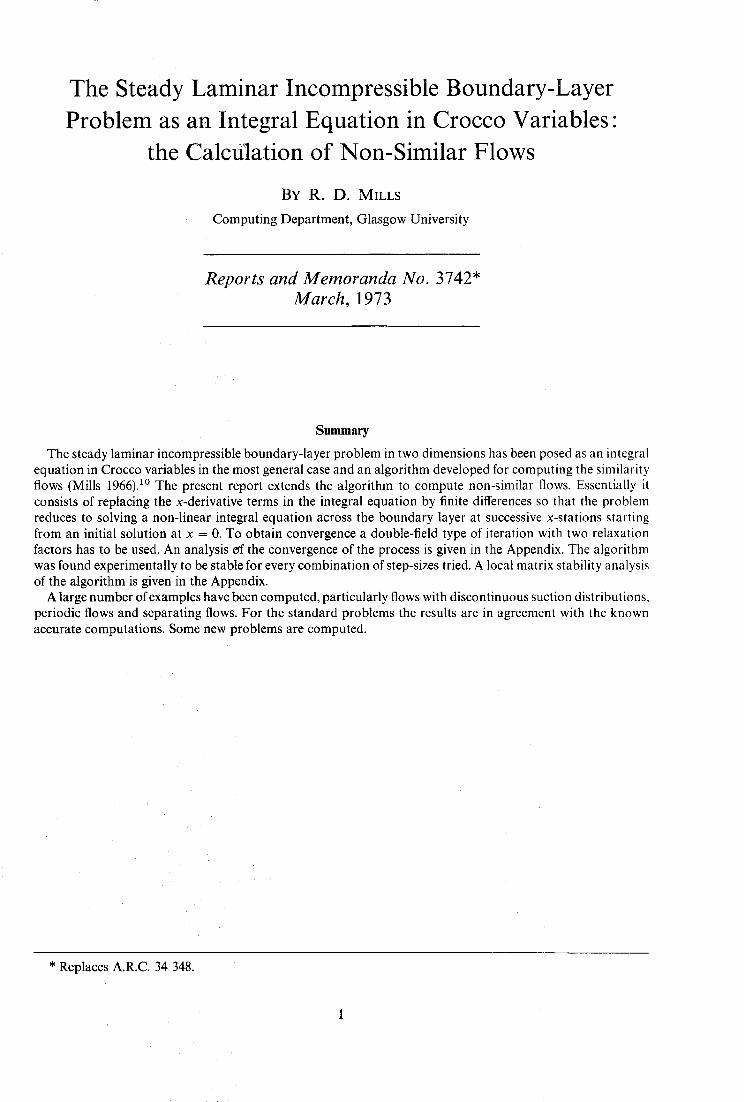
Summary The steady laminar incompressible boundary-layer problem in two dimensions has been posed as an integral

equation in Crocco variables in the most general case and an algorithm developed for computing the similarity flows (Mills 1966). 1° The present report extends the algorithm to compute non-similar flows. Essentially it consists of replacing the x-derivative terms in the integral equation by finite differences so that the problem reduces to solving a non-linear integral equation across the boundary layer at successive x-stations starting from an initial solution at x = 0. To obtain convergence a double-field type of iteration with two relaxation factors has to be used. An analysis of the convergence of the process is given in the Appendix. The algorithm was found experimentally to be stable for every combination of step-sizes tried. A local matrix stability analysis of the algorithm is given in the Appendix.

A large number of examples have been computed, particularly flows with discontinuous suction distributions, periodic flows and separating flows. For the standard problems the results are in agreement with the known accurate computations. Some new problems are computed.

* Replaces A.R.C. 34 348.

LIST OF CONTENTS

1. Introduction

2. Integral Equation Formulation of the Boundary-Layer Problem

2.1. Weakening the singularities 2.2. Boundary-Layer characteristics

3. Method of Solution of the Integral Equation

3.1. Solution technique

4. Examples

4.1. Discontinuous boundary-layer flows

4.2. Periodic boundary-layer flows

4.3. Flows with separation

5. Concluding Remarks

Acknowledgments

References

Appendix--

A1. Convergence of the iterative processes

AI. 1. Simplified problem

A1.2. Integral-equation problem

A2. Stability

A2.1. An explicit-type scheme

A2.2. Implicit scheme

Tables 1 and 2

Illustrations Figs. 1 to 13

Detachable Abstract Cards

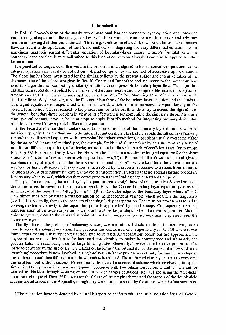
1. Introduction

In Ref. 10 Crocco's form of the steady two-dimensional laminar boundary-layer equation was converted into an integral equation in the most general case of arbitrary mainstream pressure distribution and arbitrary suction or blowing distributions at the wall. This is a generalisation of a well-known result for constant-pressure flow. In fact, it is the application of the Picard method for integrating ordinary differential equations to the non-linear parabolic partial differential equation of boundary-layer theory. Crocco's formulation of the boundary-layer problem is very well suited to this kind of conversion, though it can also be applied to other formulations.

The practical consequence of this work is the provision of an algorithm for numerical computation, as the integral equation can readily be solved on a digital computer by the method of successive approximation. The algorithm has been investigated for the similarity flows by the present author and extensive tables of the characteristics of these flows are given in Ref. 10. Cohen and Reshotko 2 had, unknown to the present author, used this algorithm for computing similarity solutions in compressible boundary-layer flow. The algorithm has also been successfully applied to the problem of the compressible and incompressible mixing of two parallel streams (see Ref. 12). This same idea had been used by Wey125 for computing some of the incompressible similarity flows. Weyl, however, used the Falkner-Skan form of the boundary-layer equation and this leads to an integral equation with exponential terms in its kernel, which is not so attractive computationally as the present formulation. Thus it seemed to the present author to be worth while to try to extend the algorithm to the general boundary-layer problem in view of its effectiveness for computing the similarity flows. Also, in a more general context, it would be an attempt to apply Picard's method for integrating ordinary differential equations to a well-known partial differential equation.

In the Picard algorithm the boundary conditions on either side of the boundary layer do not have to be satisfied explicitly; they are 'built-in' to the integral equation itself. This feature avoids the difficulties of solving a non-linear differential equation with 'two-point' boundary conditions, a problem usually overcome either by the so-called 'shooting' method (see, for example, Smith and Clutter 2°) or by solving iteratively a set of non-linear difference equations, often having an associated tridiagonal matrix of coefficients (see, for example, Fox, 3, p. 86). For the similarity flows, the Picard method leads to a non-linear integral equation for the shear stress as a function of the transverse velocity-ratio u* = u/U(x). For non-similar flows the method gives a non-linear integral equation for the shear stress as a function of u* and x when the x-derivative terms are replaced by finite differences. This equation is then solved by iteration at successive x-stations from an initial solution at x0. A preliminary Falkner-Skan-type transformation is used so that no special starting procedure is necessary when x o = 0, which can then correspond to a sharp leading edge or a stagnation point.

This plan for computing the boundary-layer equation seems straightforward and attractive. Several practical difficulties arise, however, in the numerical work. First, the Crocco boundary-layer equation possesses a singularity of the type (1 - u*)[log {(1 - u*)-l}] ~ at the outer edge of the boundary layer where u* = 1. This difficulty is met by using a transformation of the independent variable which weakens the singularity (see Ref. 10). Secondly, there is the problem of the singularity at separation. The iteration process was found to converge" extremely slowly if the separation point is approached by small x-steps. Consequently a special representation of the x-derivative terms was used to allow larger steps to be taken near separation. Also, in order to get very close to the separation point, it was found necessary to use a very small step-size across the boundary layer.

Thirdly, there is the problem of achieving convergence, and at a satisfactory rate, in the iterative process used to solve the integral equation. This problem was considered only superficially in Ref. 10 where it was found experimentally that 'under-relaxation' had to be used. As 'separation' conditions are approached the degree of under-relaxation has to be increased considerably to maintain convergence and ultimately the process fails, the same being true for large blowing rates. Generally, however, the iterative process can be made to converge by the use of a single relaxation factor og.t Unfortunately for the non-similar flows, where a 'marching' procedure is now involved, a single-relaxation-factor process works only for one or two steps in the x-direction and then fails no matter how much 0 is reduced. The author tried many artifices to overcome this problem, but without success. He eventually discovered a successful scheme which involves splitting the simple iteration process into two simultaneous processes with two relaxation factors o9 and o9'. The author was led to this idea through working on the full Navier-Stokes equations (Ref. 13) and using the 'two-field' iteration technique of Thom.2 2 Reasons for the failure of the simple scheme and the success of the double-field scheme are advanced in the Appendix, though they were not understood by the author when he first succeeded

t The relaxation factor is denoted by o9 in this report to conform with the usual notation for such factors.

in getting the method to work. The basic iterative scheme was accelerated by the well-known Aitken technique and this frequently results in savings of over 25 per cent in the number of iterations. Another benefit of the accelerated scheme is that one can obtain convergence closer to the separation point than with the unaccelerated scheme.

Lastly, there is the problem of the stability of the marching process in the x-direction. It is well known that implicit difference methods for linear parabolic partial differential equations are unconditionally stable while explicit methods are conditionally stable. For non-linear problems it is necessary to consider local stability whereby the non-linear problem is linearized and the stability of the linearized problem taken to be representa- tive locally of the stability of the full non-linear problem. The present difference representation of the boundary- layer problem is of implicit type and one would expect unconditional stability. The method was found experi- mentally to be stable for all the combinations of step-sizes in the streamwise and transverse directions that were tried. A local matrix stability analysis is given in the Appendix in support of this experimental evidence. In addition, a simple explicit-type scheme was tried and found to become rapidly unstable for every combination of step sizes used. A stability analysis of this scheme shows that instability will occur as x increases for any fixed combination of step sizes. This result is unfortunate since the explicit scheme avoids to a large extent the con- vergency difficulties of the implicit scheme.

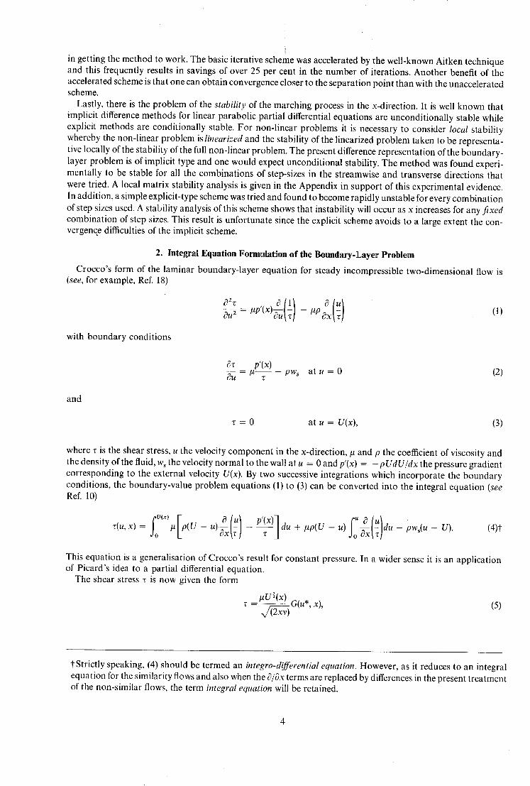
2. Integral Equation Formulation of the Boundary-Layer Problem

Crocco's form of the laminar boundary-layer equation for steady incompressible two-dimensional flow is (see, for example, Ref. 18)

Ou 2 - up'(x) - Up~x ~ (1)

with boundary conditions

and

& p'(x) --Ou = # 3 - p w , a t u = O (2)

z = 0 at u = U(x), (3)

where z is the shear stress, u the velocity component in the x-direction, # and p the coefficient of viscosity and the density of the fluid, w s the velocity normal to the wall at u = 0 and p'(x) = - pUdU/dx the pressure gradient corresponding to the external velocity U(x). By two successive integrations which incorporate the boundary conditions, the boundary-value problem equations (1) to (3) can be converted into the integral equation (see Ref. 10)

(4)t

This equation is a generalisation of Crocco's result for constant pressure. In a wider sense it is an application of Picard's idea to a partial differential equation.

The shear stress ~ is now given the form

- I~U~(X)-G'u*, x), (5)

? Strictly speaking, (4) should be termed an integro-differential equation. However, as it reduces to an integral equation for the similarity flows and also when the ~3/Ox terms are replaced by differences in the present treatment of the non-similar flows, the term integral equation will be retained.

4

where

u* = u/U(x) (6)

and v = #/p is the kinematic viscosity coefficient of the fluid. This preliminary Falkner-Skan-type trans- formation removes the awkward leading-edge singularity from the formulation of the problem. (Note that the normalisation with respect to x has been altered from the more general type used in Ref. 10 as the latter is not so convenient for non-similar problems. In fact, if the length g(x) in Ref. I0 is replaced by ( x / ~ / U ) then the shear stress function F(u*) of Ref. 10 becomes identical with the above (G(u*)). The class of 'similarity' flows has external velocity distributions U(x) and suction or blowing velocity distributions %(x) such that G becomes a function of u* only.

Substitution of (5) and (6) into (4) leads to the following integral equation for G(x, u*):

2P + (1 + P)u* - (1 + 3P)u .2 G(u*, X)

, G

where

foe + (1 - u*) (1 + P)u* G + 2u*x du* ÷ W(x)(1 - u*), (7)

P(x) - U dx and W(x) = Ws(X ) ~ . (8)

2 .1 . W e a k e n i n g t h e S i n g u l a r i t i e s

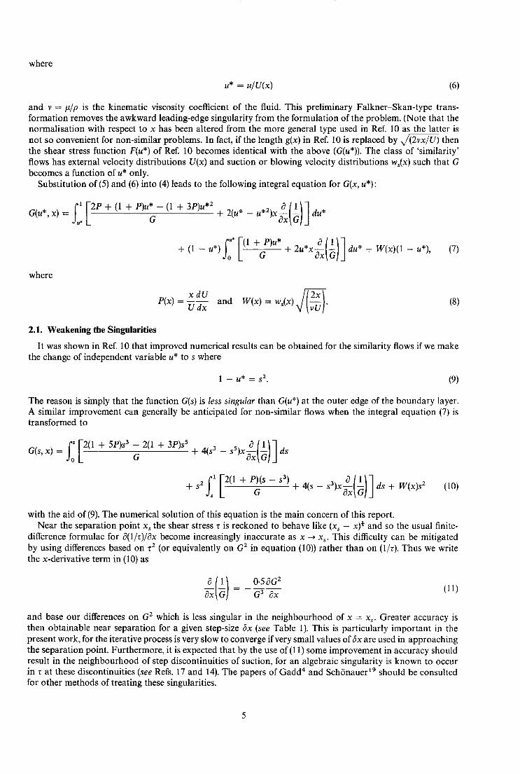
It was shown in Ref. 10 that improved numerical results can be obtained for the similarity flows if we make the change of independent variable u* to s where

1 - u* = s 2. (9)

The reason is simply that the function G(s) is less singular than G(u*) at the outer edge of the boundary layer. A similar improvement can generally be anticipated for non-similar flows when the integral equation (7) is transformed to

+ s 2 + 4(s - s3)x ds + W(x)s 2 (10) G

with the aid of (9). The numerical solution of this equation is the main concern of this report. Near the separation point xs the shear stress r is reckoned to behave like (Xs - x) ~ and so the usual finite-

difference formulae for a(1/z)/Ox become increasingly inaccurate as x ~ x~. This difficulty can be mitigated by using differences based on z 2 (or equivalently on G 2 in equation (10)) rather than on (l/z). Thus we write the x-derivative term in (10) as

0 ( 1 ) 0.5OG z (11) 7x -G = G 3 Ox

and base our differences o n G 2 which is less singular in the neighbourhood of x = xs. Greater accuracy is then obtainable near separation for a given step-size 6x (see Table 1). This is particularly important in the present work, for the iterative process is very slow to converge if very small values of 6x are used in approaching the separation point. Furthermore, it is expected that by the use of (11) some improvement in accuracy should result in the neighbourhood of step discontinuities of suction, for an algebraic singularity is known to occur in z at these discontinuities (see Refs. 17 and 14). The papers of Gadd 4 and Schdnauer 19 should be consulted for other methods of treating these singularities.

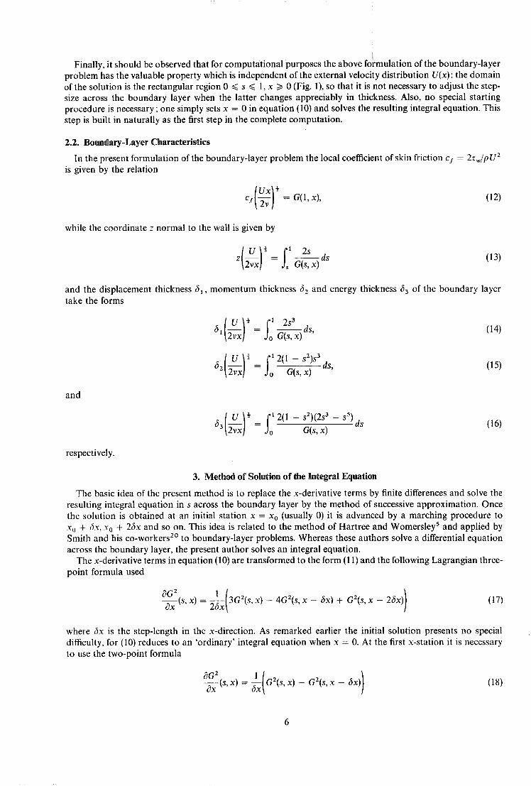
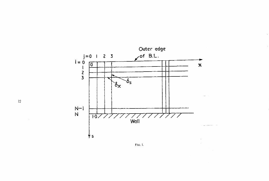
Finally, it should be observed that for computational purposes the above formulation of the boundary-layer problem has the valuable property which is independent of the external velocity distribution U(x): the domain of the solution is the rectangular region 0 ~< s ~< 1, x >/0 (Fig. 1), so that it is not necessary to adjust the step- size across the boundary layer when the latter changes appreciably in thickness. Also, no special starting procedure is necessary ; one simply sets x = 0 in equation (10) and solves the resulting integral equation. This step is built in naturally as the first step in the complete computation.

2.2. Boundary-Layer Characteristics

In the present formulation of the boundary-layer problem the local coefficient of skin friction cy = 2zw/pU 2 is given by the relation

[ Uxl ½ cy[~V-v ] = G(1,x), (12)

while the coordinate z normal to the wall is given by

z = s ~ d s (13)

and the displacement thickness 61 , momentum thickness 6 2 and energy thickness 6 3 of the boundary layer take the forms

f; 61 = G--~,x~ dS, (14)

62 = o G(s,x) ds, (15)

and

( u )~ = j ' 1 2 ( 1 - s2)(2s3 - sS) 63 ~VX o G(s, x) ds (16)

respectively.

3. Method of Solution of the Integral Equation

The basic idea of the present method is to replace the x-derivative terms by finite differences and solve the resulting integral equation in s across the boundary layer by the method of successive approximation. Once the solution is obtained at an initial station x = Xo (usually 0) it is advanced by a marching procedure to x o + 6x, x o + 26x and so on. This idea is related to the method of Hartree and Womersley s and applied by Smith and his co-workers 2° to boundary-layer problems. Whereas these authors solve a differential equation across the boundary layer, the present author solves an integral equation.

The x-derivative terms in equation (10) are transformed to the form (11) and the following Lagrangian three- point formula used

where fix is the step-length in the x-direction. As remarked earlier the initial solution presents no special difficulty, for (10) reduces to an 'ordinary' integral equation when x = 0. At the first x-station it is necessary to use the two-point formula

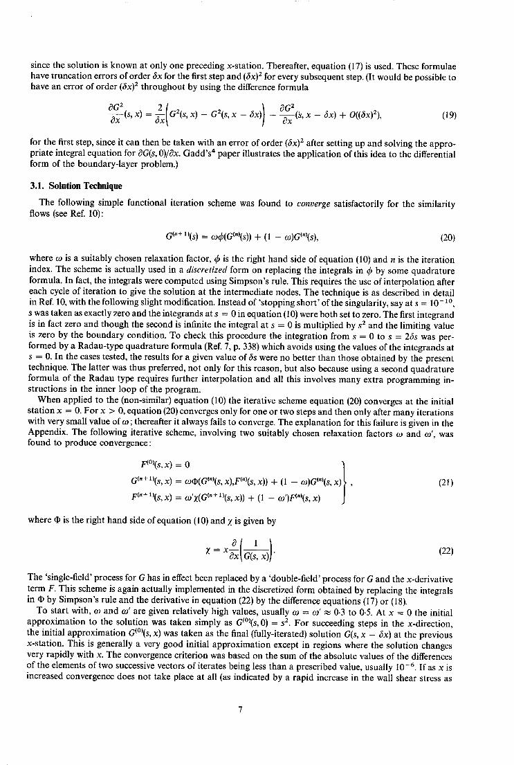
since the solution is known at only one preceding x-station. Thereafter, equation (17) is used. These formulae have truncation errors of order 6x for the first step and (6x) 2 for every subsequent step. (It would be possible to have an error of order (6x) 2 throughout by using the difference formula

OG-~2(S'X)ox = 2 (a2( s , x ) _ a2(s,x - (~x)) - oa2('s,x 6x) + 0((6x)2) , (19)

for the first step, since it can then be taken with an error of order (6x) 2 after setting up and solving the appro- priate integral equation for 8G(s, O)/Ox. Gadd's 4 paper illustrates the application of this idea to the differential form of the boundary-layer problem.)

3.1. Solution Technique

The following simple functional iteration scheme was found to converge satisfactorily for the similarity flows (see Ref. 10):

G ~"+ l~(s) -~ og~(G~")(s)) q- (1 - og)G~")(s), (20)

where 09 is a suitably chosen relaxation factor, q~ is the right hand side of equation (10) and n is the iteration index. The scheme is actually used in a discretized form on replacing the integrals in 4) by some quadrature formula. In fact, the integrals were computed using Simpson's rule. This requires the use of interpolation after each cycle of iteration to give the solution at the intermediate nodes. The technique is as described in detail in Ref. 10, with the following slight modification. Instead of 'stopping short ' of the singularity, say at s = 10- ~o, s was taken as exactly zero and the integrands at s = 0 in equation (10) were both set to zero. The first integrand is in fact zero and though the second is infinite the integral at s = 0 is multiplied by s 2 and the limiting value is zero by the boundary condition. To check this procedure the integration from s = 0 to s = 26s was per- formed by a Radau-type quadrature formula (Ref. 7, p. 338) which avoids using the values of the integrands at s = 0. In the cases tested, the results for a given value of 6s were no better than those obtained by the present technique. The latter was thus preferred, not only for this reason, but also because using a second quadrature formula of the Radau type requires further interpolation and all this involves many extra programming in- structions in the inner loop of the program.

When applied to the (non-similar) equation (10) the iterative scheme equation (20) converges at the initial station x = 0. For x > 0, equation (20) converges only for one or two steps and then only after many iterations with very small value of o9; thereafter it always fails to converge. The explanation for this failure is given in the Appendix. The following iterative scheme, involving two suitably chosen relaxation factors o9 and o9', was found to produce convergence:

Ft°)(s, x) = 0 ]

G ("+ 1)(s, x) = og¢o(G(")(s, x),F~")(s, x)) + (1 - co)G~")(s, x ) l '

F c"+ L)(s, x) O9'z(G ("+ 1)(s, x)) --[- (1 - O9')F~")(s, x)

(21)

where ~ is the right hand side of equation (10) and X is given by

Z = 8x~G(s, x)]" (22)

The 'single-field' process for G has in effect been replaced by a 'double-field' process for G and the x-derivative term F. This scheme is again actually implemented in the discretized form obtained by replacing the integrals in • by Simpson's rule and the derivative in equation (22) by the difference equations (17) or (18).

To start with, 09 and co' are given relatively high values, usually ~o = co' ,~ 0.3 to 0.5. At x = 0 the initial approximation to the solution was taken simply as Gt°)(s, 0) = s 2. For succeeding steps in the x-direction, the initial approximation G~°~(s, x) was taken as the final (fully-iterated) solution G(s, x - fix) at the previous x-station. This is generally a very good initial approximation except in regions where the solution changes very rapidly with x. The convergence criterion was based on the sum of the absolute values of the differences of the elements of two successive vectors of iterates being less than a prescribed value, usually 10 -6. If as x is increased convergence does not take place at all (as indicated by a rapid increase in the wall shear stress as

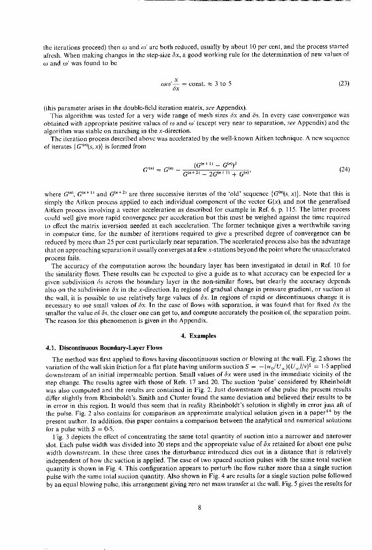
the iterations proceed) then co and co' are both reduced, usually by about 10 per cent, and the process started afresh. When making changes in the step-size f x , a good working rule for the determination of new values of co and co' was found to be

X cocO'~x x = const. ~ 3 to 5 (23)

(this parameter arises in the double-field iteration matrix, see Appendix). This algorithm was tested for a very wide range of mesh sizes fix and fs. In every case convergence was

obtained with appropriate positive values of co and e)' (except very near to separation, see Appendix) and the algorithm was stable on marching in the x-direction.

The iteration process described above was accelerated by the well-known Aitken technique. A new sequence of iterates {G'(")(s, x)} is formed from

G,~.~ = G ( . ) _ (G ~"+1) - G(")) 2 G~n+2) __ 2G(,+ 1) + G~,) ,

(24)

where G ~"), G ~"+ 1) and G ~n+2) a r e three successive iterates of the 'old' sequence {G~")(s, x)}. Note that this is simply the Aitken process applied to each individual component of the vector G(x), and not the generalised Aitken process involving a vector acceleration as described for example in Ref. 6, p. 115. The latter process could well give more rapid convergence per acceleration but this must be weighed against the time required to effect the matrix inversion needed at each acceleration. The former technique gives a worthwhile saving in computer time, for the number of iterations required to give a prescribed degree of convergence can be reduced by more than 25 per cent particularly near separation. The accelerated process also has the advantage that on approaching separation it usually converges at a few x-stations beyond the point where the unaccelerated process fails.

The accuracy of the computation across the boundary layer has been investigated in detail in Ref. 10 for the similarity flows. These results can be expected to give a guide as to what accuracy can be expected for a given subdivision 6s across the boundary layer in the non-similar flows, but clearly the accuracy depends also on the subdivision fx in the x-direction. In regions of gradual change in pressure gradient, or suction at the wall, it is possible to use relatively large values of fx . In regions of rapid or discontinuous change it is necessary to use small values of fx . In the case of flows with separation, it was found that for fixed f x the smaller the value of fs, the closer one can get to, and compute accurately the position of, the separation point. The reason for this phenomenon is given in the Appendix.

4. E x a m p l e s

4.1. D i scont inuous Boundary-Layer Flows

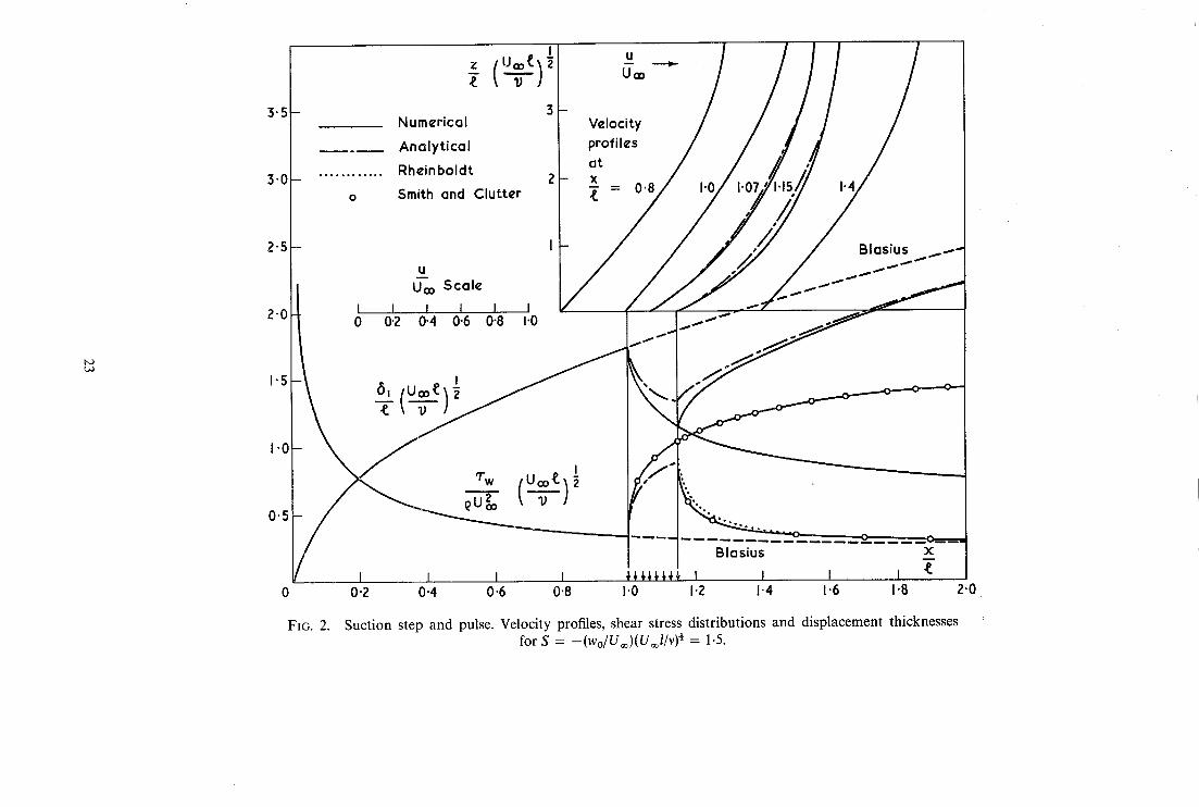
The method was first applied to flows having discontinuous suction or blowing at the wall. Fig. 2 shows the variation of the wall skin friction for a fiat plate having uniform suction S = - (wo/U~)(U~l /v )~ = 1-5 applied downstream of an initial impermeable portion. Small values of 6x were used in the immediate vicinity of the step change. The results agree with those of Refs. 17 and 20. The suction 'pulse' considered by Rheinboldt was also computed and the results are contained in Fig. 2. Just downstream of the pulse the present results differ slightly from Rheinboldt's. Smith and Clutter found the same deviation and believed their results to be in error in this region. It would thus seem that in reality Rheinboldt's solution is slightly in error just aft of the pulse. Fig. 2 also contains for comparison an approximate analytical solution given in a paper 14 by the present author. In addition, this paper contains a comparison between the analytical and numerical solutions for a pulse with S = 0-5.

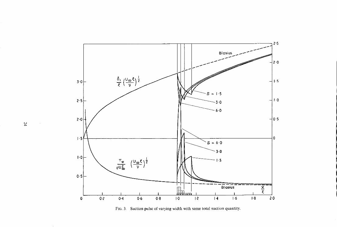
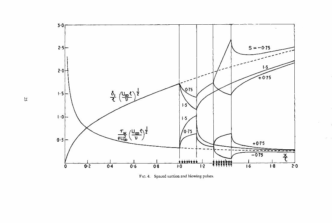
Fig. 3 depicts the effect of concentrating the same total quantity of suction into a narrower and narrower slot. Each pulse width was divided into 20 steps and the appropriate value of 3x retained for about one pulse width downstream. In these three cases the disturbance introduced dies out in a distance that is relatively independent of how the suction is applied. The case of two spaced suction pulses with the same total suction quantity is shown in Fig. 4. This configuration appears to perturb the flow rather more than a single suction pulse with the same total suction quantity. Also shown in Fig. 4 are results for a single suction pulse followed by an equal blowing pulse, this arrangement giving zero net mass transfer at the wall. Fig. 5 gives the results for

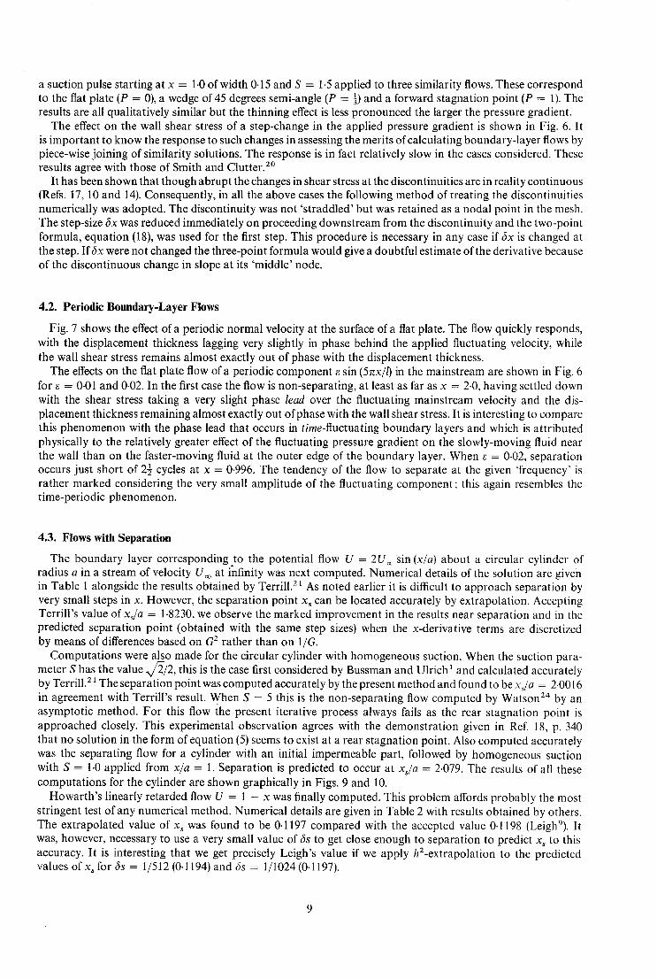
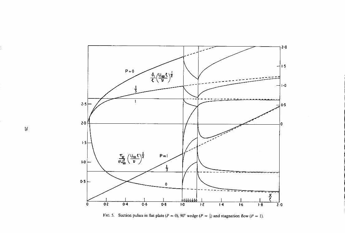
a suction pulse starting at x = 1.0 of width 0.15 and S = 1.5 applied to three similarity flows. These correspond to the flat plate (P = 0), a wedge of 45 degrees semi-angle (P = 1) and a forward stagnation point (P = 1). The results are all qualitatively similar but the thinning effect is less pronounced the larger the pressure gradient.

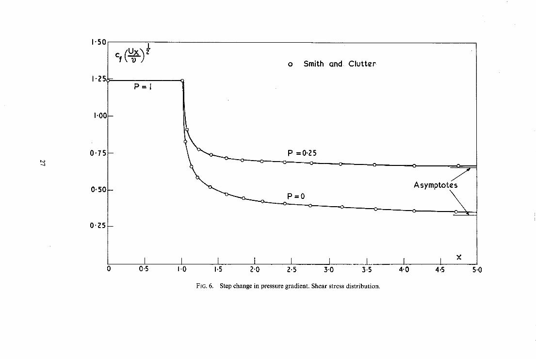
The effect on the wall shear stress of a step-change in the applied pressure gradient is shown in Fig. 6. It is important to know the response to such changes in assessing the merits of calculating boundary-layer flows by piece-wise joining of similarity solutions. The response is in fact relatively slow in the cases considered. These results agree with those of Smith and Clutter. z°

It has been shown that though abrupt the changes in shear stress at the discontinuities are in reality continuous (Refs. 17, 10 and 14). Consequently, in all the above cases the following method of treating the discontinuities numerically was adopted. The discontinuity was not 'straddled' but was retained as a nodal point in the mesh. The step-size 3x was reduced immediately on proceeding downstream from the discontinuity and the two-point formula, equation (18), was used for the first step. This procedure is necessary in any case if 6x is changed at the step. If6x were not changed the three-point formula would give a doubtful estimate of the derivative because of the discontinuous change in slope at its 'middle' node.

4.2. Periodic Boundary-Layer Flows

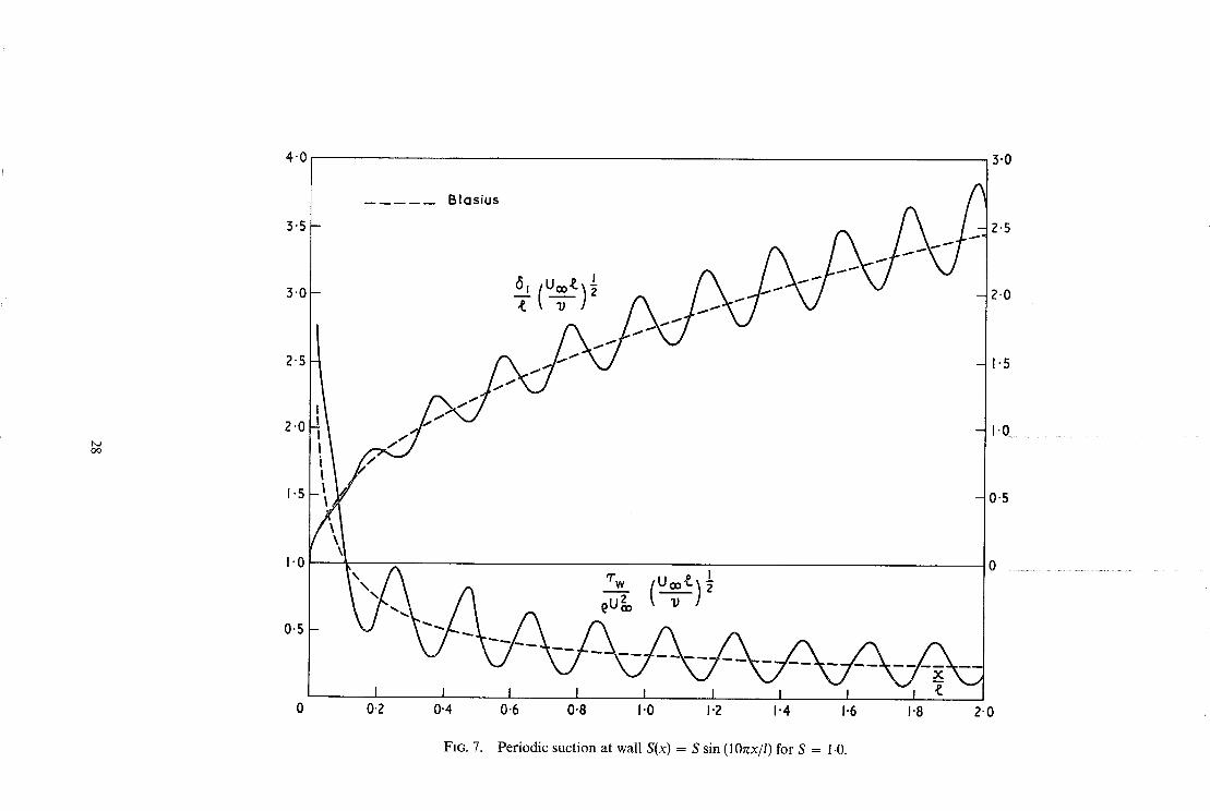
Fig. 7 shows the effect of a periodic normal velocity at the surface of a fiat plate. The flow quickly responds, with the displacement thickness lagging very slightly in phase behind the applied fluctuating velocity, while the wall shear stress remains almost exactly out of phase with the displacement thickness.

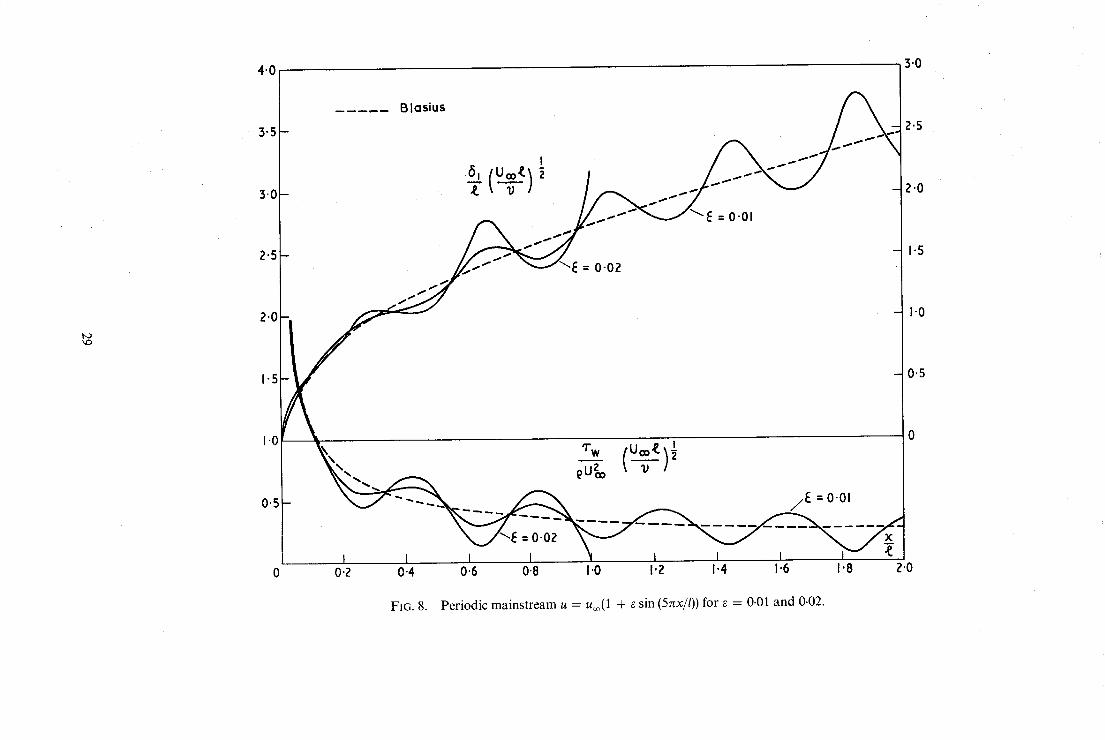
The effects on the fiat plate flow of a periodic component t sin (5nx/l) in the mainstream are shown in Fig. 6 for ~ = 0.01 and 0.02. In the first case the flow is non-separating, at least as far as x = 2.0, having settled down with the shear stress taking a very slight phase lead over the fluctuating mainstream velocity and the dis- placement thickness remaining almost exactly out of phase with the wall shear stress. It is interesting to compare this phenomenon with the phase lead that occurs in time-fluctuating boundary layers and which is attributed physically to the relatively greater effect of the fluctuating pressure gradient on the slowly-moving fluid near the wall than on the faster-moving fluid at the outer edge of the boundary layer. When ~ = 0.02, separation occurs just short of 2½ cycles at x = 0.996. The tendency of the flow to separate at the given 'frequency' is rather marked considering the very small amplitude of the fluctuating component ; this again resembles the time-periodic phenomenon.

4.3. Flows with Separation

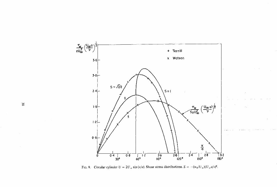
The boundary layer corresponding to the potential flow U = 2U~. sin (x/a) about a circular cylinder of radius a in a stream of velocity U~ at infinity was next computed. Numerical details of the solution are given in Table 1 alongside the results obtained by Terrill. z 1 As noted earlier it is difficult to approach separation by very small steps in x. However, the separation point x s can be located accurately by extrapolation. Accepting Terrill's value of xJa = 1-8230, we observe the marked improvement in the results near separation and in the predicted separation point (obtained with the same step sizes) when the x-derivative terms are discretized by means of differences based on G z rather than on 1/G.

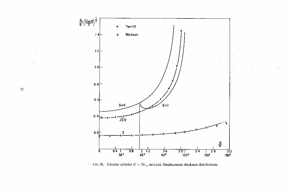
Computations were also made for the circular cylinder with homogeneous suction. When the suction para- meter S has the value x//2/2, this is the case first considered by Bussman and Ulrich 1 and calculated accurately by Terrill. 21 The separation point was computed accurately by the present method and found to be x j a = 2.0016 in agreement with Terrill's result. When S = 5 this is the non-separating flow computed by Watson 24 by an asymptotic method. For this flow the present iterative process always fails as the rear stagnation point is approached closely. This experimental observation agrees with the demonstration given in Ref. 18, p. 340 that no solution in the form of equation (5) seems to exist at a rear stagnation point. Also computed accurately was the separating flow for a cylinder with an initial impermeable part, followed by homogeneous suction with S = 1-0 applied from x/a = 1. Separation is predicted to occur at x j a = 2.079. The results of all these computations for the cylinder are shown graphically in Figs. 9 and 10.

Howarth's linearly retarded flow U = 1 - x was finally computed. This problem affords probably the most stringent test of any numerical method. Numerical details are given in Table 2 with results obtained by others. The extrapolated value of x s was found to be 0.1197 compared with the accepted value 0.1198 (Leigh9). It was, however, necessary to use a very small value of 6s to get close enough to separation to predict xs to this accuracy. It is interesting that we get precisely Leigh's value if we apply hZ-extrapolation to the predicted values ofx~ for 6s = 1/512 (0.1194) and 6s = 1/1024 (0.1197).

5. Concluding Remarks

The steady two-dimensional incompressible laminar boundary-layer problem has been posed as an integral equation in Crocco variables and a numerical method of solution of this problem has been developed. Several non-separating flows have been computed by the method, particularly flows with discontinuous suction dis- tributions and periodic flows. Some problems involving separation have also been computed.

Viewed as a marching procedure for solving a parabolic partial differential equation, the method is implicit and was found experimentally to be stable for all the combinations of step-sizes tried. This result is made plausible by the local stability analysis given in the Appendix. The stability of an explicit-type scheme is also examined. The crucial device required to make the method work is the double-field type of iteration for solving the integral equation. An analysis of the convergence of this process is given in the Appendix.

The method is quite simple conceptually. It is easy to program and the storage requirements are relatively small. The method was programmed throughout by the author, originally in Autocode and run on the Cam- bridge University Atlas (Titan) computer and latterly in FORTRAN and run on the Glasgow University KDF9 computer and on the Univac 1108 computer at the National Engineering Laboratory. To give an indication of computing times, it was found that with a step-size Js = 1/64 across the boundary layer the time to compute and print at each of 22 x-stations the velocity profiles, the boundary-layer characteristics c f, J l , ~2 and 33 and to predict the separation point to about 0.5 per cent for the circular cylinder was about 30 seconds on the Univac, an average of about 1-4 seconds per station.

Acknowledgements

This work was started while the author held an ICI Research Fellowship in the Aeronautics Laboratory of the Cambridge University Engineering Department. The author would like to express his indebtedness to Pro- fessor W. A. Mair for the facilities extended to him and for his interest in the work. The author gratefully acknowledges the receipt of the necessary computer time for this investigation on the Cambridge University Titan computer, the Glasgow University KDF9 computer and the finance from the S.R.C. for the time on the National Engineering Laboratory Univac 1108 computer.

10

No. Author(s)

1 K. Bussmann and A. Ulrich

2 C.B. Cohen and E. Reshotko . .

3 L. Fox . . . . . . . .

4 G . E . Gadd

5 D . R . Hartree and J. R. Womersley

6 P. Henrici . . . . . . . .

7 F .B. Hildebrand . . . . . .

8 E. Isaacson and H. B. Keller . .

9 D . C . F . Leigh . . . . . .

10 R .D. Mills . . . . . . . .

11 R.D. Mills . . . . . . . .

12 R .D. Mills . . . . . . . .

13 R .D. Mills . . . . . . . .

14 R .D. Mills . . . . . . . .

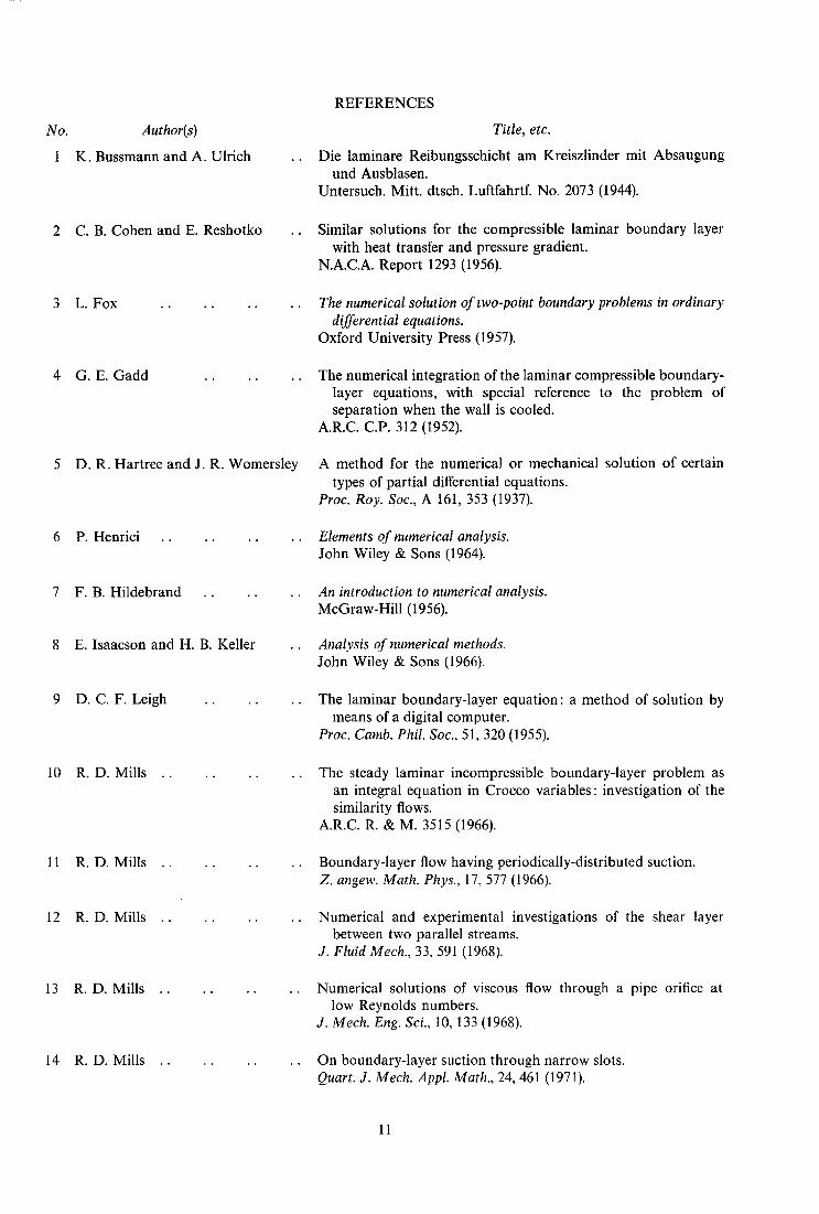
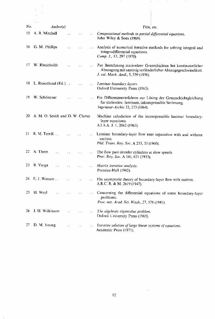
REFERENCES

Title, etc.

Die laminate Reibungsschicht am Kreiszlinder mit Absaugung und Ausblasen.

Untersuch. Mitt. dtsch. Luftfahrtf. No. 2073 (1944).

Similar solutions for the compressible laminar boundary layer with heat transfer and pressure gradient.

N.A.C.A. Report 1293 (1956).

The numerical solution of two-point boundary problems in ordinary differential equations.

Oxford University Press (1957).

The numerical integration of the laminar compressible boundary- layer equations, with special reference to the problem of separation when the wall is cooled.

A.R.C.C.P. 312 (1952).

A method for the numerical or mechanical solution of certain types of partial differential equations.

Proc. Roy. Soc., A 161,353 (1937).

Elements of numerical analysis. John Wiley & Sons (1964).

An introduction to numerical analysis. McGraw-Hill (1956).

Analysis of numerical methods. John Wiley & Sons (1966).

The laminar boundary-layer equation: a method of solution by means of a digital computer.

Proc. Camb. Phil. Soc., 51,320 (1955).

The steady laminar incompressible boundary-layer problem as an integral equation in Crocco variables: investigation of the similarity flows.

A.R.C.R. & M. 3515 (1966).

Boundary-layer flow having periodically-distributed suction. Z. angew. Math. Phys., 17, 577 (1966).

Numerical and experimental investigations of the shear layer between two parallel streams.

J. Fluid Mech., 33, 591 (1968).

Numerical solutions of viscous flow through a pipe orifice at low Reynolds numbers.

J. Mech. Eng. Sci., 10, 133 (1968).

On boundary-layer suction through narrow slots. Quart. J. Mech. Appl. Math., 24, 461 (1971).

11

/

No. Author(s)

15 A.R. Mitchell

16 G .M. Phillips . . . .

17 W. Rheinboldt

18 L. Rosenhead (Ed.) . ..

19 W. Sch6nauer

20 A . M . O . Smith and D. W. Clutter

21 R.M. Terrill . . . . . . . .

22 A. Thom . . . . . . . .

23 R. Varga . . . . . . . .

24 E.J. Watson . . . .

25 H. Weyl ..

26 J .H. Wilkinson

27 D.M. Young

Title, etc.

Computational methods in partial differential equations. John Wiley & Sons (1969).

Analysis of numerical iterative methods for solving integral and integrodifferential equations.

Comp. J., 13, 297 (1970).

Zur Berechnung stationgrer Grenzchichten bei kontinuierlicher Absaugung mit unstetig verl~inderlicher Absaugegeschwindikeit.

J. rat. Mech. Anal., 5, 539 (1956).

Laminar boundary layers. Oxford University Press (1963).

Ein Differenzenverfahren zur L6sing der Grenzschichtgleichung fiir station~ire, laminare, inkompressible Str6mung.

lngenieur-Arehiv 33, 173 (1964).

Machine calculation of the incompressible laminar boundary- layer equations.

A.I.A.A.J. 1, 2062 (1963).

Laminar boundary-layer flow near separation with and without suction.

Phil. Trans. Roy. Soc. A 253, 55 (1960).

The flow past circular cylinders at slow speeds. Proc. Roy. Soc. A 141,651 (1933).

Matrix iterative analysis. Prentice-Hall (1962).

The asymptotic theory of boundary-layer flow with suction. A.R.C.R. & M. 2619 (1947).

Concerning the differential equations of some boundary-layer problems.

Proc. nat. Acad. Sci. Wash., 27,578 (1941).

The algebraic eigenvalue problem. Oxford University Press (1965).

lterative solution of large linear systems of equations. Academic Press (1971).

12

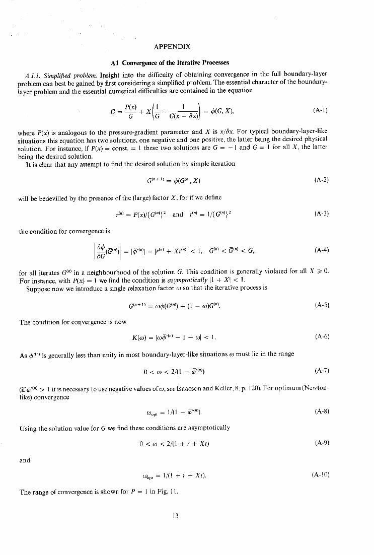
A P P E N D I X

A1 Convergence of the Iterative Processes

A.I.1. Simplified problem. Insight into the difficulty of obta ining convergence in the full boundary- layer p rob lem can best be gained by first considering a simplified problem. The essential character of the boundary- layer p rob lem and the essential numerical difficulties are contained in the equat ion

G = ~ + X ~ G(x - 6x) = (o(G,X), (A-l)

where P(x) is analogous to the pressure-gradient pa rame te r and X is x/6x. For typical boundary- layer- l ike si tuations this equat ion has two solutions, one negative and one positive, the latter being the desired physical solution. For instance, if P(x) = const. = 1 these two solutions are G = - 1 and G = t for all X, the latter being the desired solution.

I t is clear that any a t tempt to find the desired solution by simple i teration

G(,+ 1) = q~(G(,), X) (A-2)

will be bedevilled by the presence of the (large) factor X, for if we define

the condi t ion for convergence is

r(")=P(x)/{G(")} z and t ( . )= 1/{G(")} 2 (A-3)

(?q~,~(.),L I j:(") x[(") I < < < G, ~--~¢o )1 = I~'<")1 = + 1, G (") (7") (A-4)

for all iterates G (") in a ne ighbourhood of the solution G. This condi t ion is generally violated for all X >/0. For instance, with P(x) = 1 we find the condi t ion is asymptotically [1 + XI < 1.

Suppose now we introduce a single relaxat ion factor co so that the i terative process is

The condit ion for convergence is now

G(.+ l) = co~b(G(.)) + (1 - co)G ("). (A-5)

K(co) = Ico~ '(") + 1 - col < 1. (A-6)

As q~'(') is generally less than unity in most boundary- layer- l ike si tuations co must lie in the range

0 < co < 2/(1 - ~'(")) (A-7)

(if q5 '(") > 1 it is necessary to use negative values of co, see Isaacson and Keller, 8, p. 120). For o p t i m u m (Newton- like) convergence

coopt-- t/(1 - qS'(")). (A-8)

Using the solution value for G we find these condit ions are asymptot ica l ly

0 < co < 2/(1 + r + Xt) (A-9)

and

coop ' = 1/(1 + r + Xt).

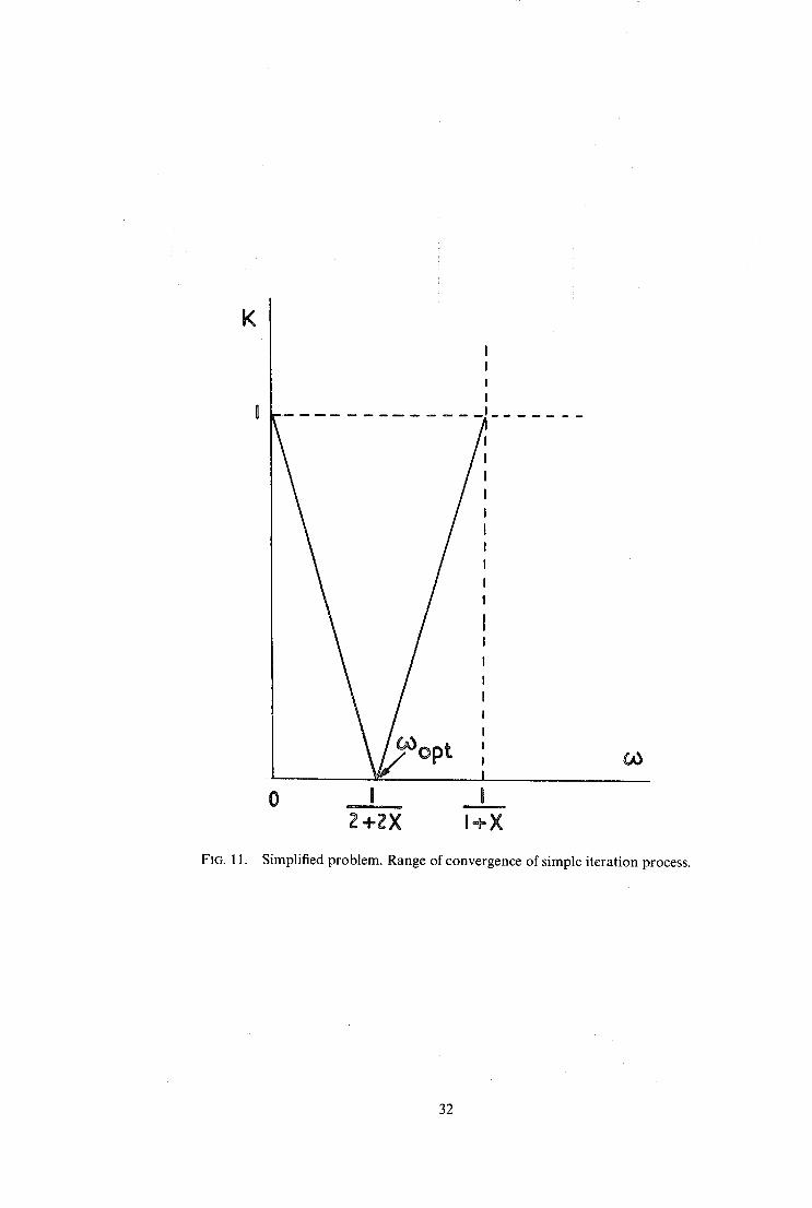
The range of convergence is shown for P = 1 in Fig. 11.

(A-10)

13

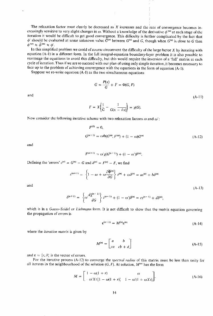
The relaxation factor must clearly be decreased as X increases and the rate of convergence becomes in- creasingly sensitive to very slight changes in o . Without a knowledge of the derivative 4) '(") at each stage of the i teration it would be difficult to get good convergence. This difficulty is further compl ica ted by the fact that ~b' should be evaluated at some unknown value (~(") between G (") and G, though when G (") is close to G then ,~'(") ~ 5 ' (" ' ~ 4,'.

In this simplified p rob lem we could of course c i rcumvent the difficulty of the large factor X by iterating with equat ion (A-l) in a different form. In the full integral-equat ion boundary- layer p rob lem it is also possible to rearrange the equat ions to avoid this difficulty, but this would require the inversion of a 'full ' matr ix at each cycle of iteration. Thus if we are to succeed with our plan of using only simple iteration, it becomes necessary to face up to the p rob lem of achieving convergence with the equat ions in the form of equat ion (A-l).

Suppose we re-write equat ion (A-l) as the two s imul taneous equat ions

P(x) G = --G- + F = (NG, F)

and (A-11)

l 1 )) = z(G). F = X G G(x 6x

N o w consider the following iterative scheme with two relaxation factors ~o and w' :

F (°) = O,

G(n+ 1) = oo(1)(G("), F ('°) + (1 - ~ )G (") (A-12)

and

F(.+ 1) = co,z(G(.+ 1)) + (1 - ~n')F (").

Defining the ' e r rors ' d ") = G (") - G and 6 (') = F (") - F, we find

e(.+ l) = I - ~o + ~ o ~ - - ; e (") + o 3 (") = ae (") + b5 (')

and (A-13)

(~(n+ 1) .= {(o d~(~+ 1)~ r. ("+ a) dG J + (1 - o ' )5 (") = ce ("+1) + d6(,),

which is in a Gauss-Seidel or Liebmann form. It is not difficult to show that the matrix equat ion governing the p ropaga t ion of errors is

r ( n + 1) : M(.¥(.) (A-14)

where the iteration matrix is given by

M(') = I a b 1 ca cb + d (A-15)

and ~ = {~., 31 is the vector of errors. For the iterative process (A-12) to converge the spectral radius of this matrix must be less than unity for

all iterates in the ne ighbourhood of the solution (G, F). At solution, M ~"J has the form

[- l - .,(1 + r) ] M = / - o ~ X t { 1 - c o ( l + r ) } t - o ' ( 1 ÷ eoXt) "

(A-16)

14

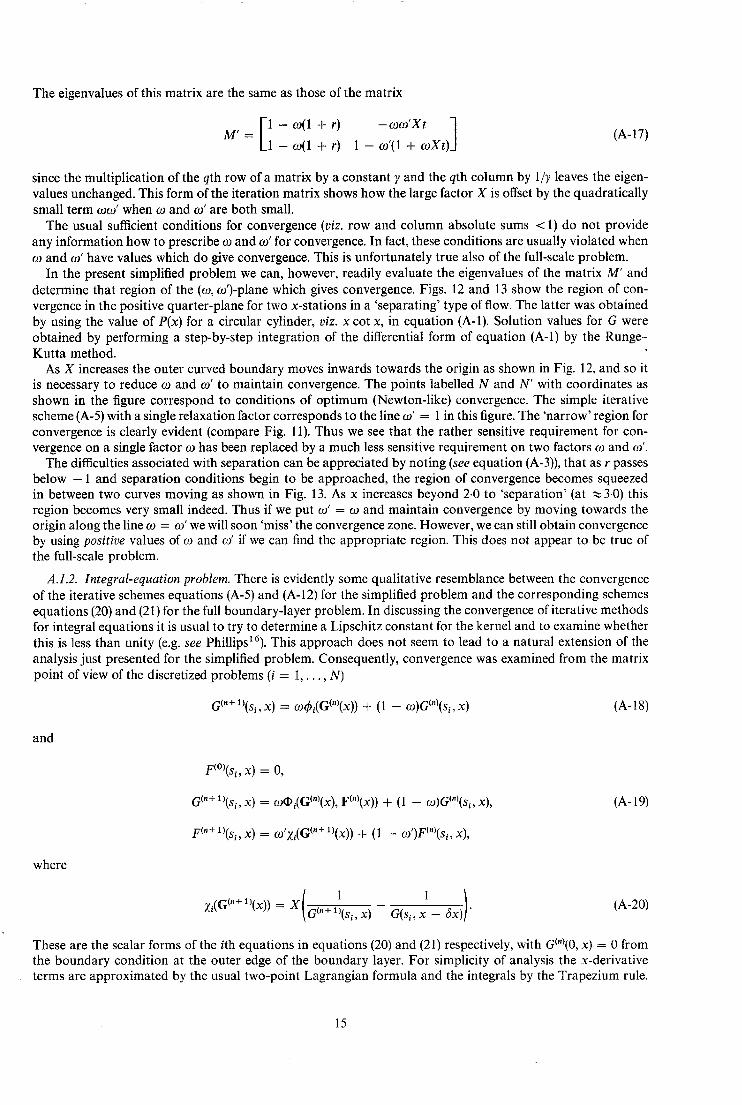
The eigenvalues of this matrix are the same as those of the matrix

M, = [11 - e)(1 + r) -coco'Xt 1 o9(1 + r) 1 - co'(1 + coXt)_]

(A-17)

since the multiplication of the qth row of a matrix by a constant y and the qth column by 1/y leaves the eigen- values unchanged. This form of the iteration matrix shows how the large factor X is offset by the quadratically small term coco' when co and co' are both small.

The usual sufficient conditions for convergence (viz. row and column absolute sums < 1) do not provide any information how to prescribe co and co' for convergence. In fact, these conditions are usually violated when co and co' have values which do give convergence, This is unfortunately true also of the full-scale problem.

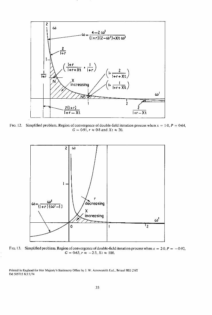
In the present simplified problem we can, however, readily evaluate the eigenvalues of the matrix M' and determine that region of the (co, e)')-plane which gives convergence. Figs. 12 and 13 show the region of con- vergence in the positive quarter-plane for two x-stations in a 'separating' type of flow. The latter was obtained by using the value of P(x) for a circular cylinder, viz. x cot x, in equation (A-I). Solution values for G were obtained by performing a step-by-step integration of the differential form of equation (A-l) by the Runge- Kutta method.

As X increases the outer curved boundary moves inwards towards the origin as shown in Fig. 12, and so it is necessary to reduce co and co' to maintain convergence. The points labelled N and N' with coordinates as shown in the figure correspond to conditions of optimum (Newton-like) convergence. The simple iterative scheme (A-5) with a single relaxation factor corresponds to the line co' = 1 in this figure. The 'narrow' region for convergence is clearly evident (compare Fig. 11). Thus we see that the rather sensitive requirement for con- vergence on a single factor co has been replaced by a much less sensitive requirement on two factors co and co'.

The difficulties associated with separation can be appreciated by noting (see equation (A-3)), that as r passes below - 1 and separation conditions begin to be approached, the region of convergence becomes squeezed in between two curves moving as shown in Fig. 13. As x increases beyond 2.0 to 'separation' (at ,~ 3.0) this region becomes very small indeed. Thus if we put co' = co and maintain convergence by moving towards the origin along the line o) = co' we will soon 'miss' the convergence zone. However, we can still obtain convergence by using positive values of co and co' if we can find the appropriate region. This does not appear to be true of the full-scale problem.

A.1.2. Integral-equation problem. There is evidently some qualitative resemblance between the convergence of the iterative schemes equations (A-5) and (A-12) for the simplified problem and the corresponding schemes equations (20) and (21) for the full boundary-layer problem. In discussing the convergence of iterative methods for integral equations it is usual to try to determine a Lipschitz constant for the kernel and to examine whether this is less than unity (e.g. see Phillips16). This approach does not seem to lead to a natural extension of the analysis just presented for the simplified problem. Consequently, convergence was examined from the matrix point of view of the discretized problems (i = i . . . . . N)

G (~+ l)(s i, x) = coq~/(G(~)(x)) + (1 - co)G~n)(si, x) (A-18)

and

F(°)(si, x) = O,

G ~+ 1)(s i, x) = CO~i(G(~)(x), F~)(x)) + (1 - co)G~')(si, x), (A- 19)

F (~+ 1)(s i, x) = co'xi(G ("+ X)(x)) + (1 - co')F(")(si, x),

where

= X 1 1 z'(G'~+~'(x)) (c~o+~(~,x) G(s,,x - 6x)) (A-20)

These are the scalar forms of the ith equations in equations (20) and (21) respectively, with G~")(0, x) = 0 from the boundary condition at the outer edge of the boundary layer. For simplicity of analysis the x-derivative terms are approximated by the usual two-point Lagrangian formula and the integrals by the Trapezium rule.

15

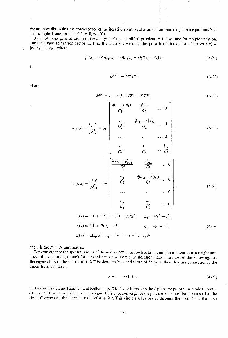
We are now discussing the convergence of the iterativ, solution of a set of non-linear algebraic equat ions (see, for example, Isaacson and Keller, 8, p. 109).

By an obvious generalisation of the analysis of the simplified problem (A.I.1) we find for simple iteration, using a single relaxation factor ~, that the matrix governing the growth of the vector of errors ~(x) = { E l , F, 2 . . . . . EN} , where

e,i~")(x) = Gt"~(si, x) - G(s~, x) = G~")(x) - Gi(x), (A-21)

is

8(n+ 1) = M~.)e~.~ (A-22)

where

M t" )= I - c o ( l

T(s [ /Jt =as

+ R oo + XTt")),

- l ( / 1 -~- Sl2nl) S2H2

l, ½(12 + s2n2) G 2 G~

. . 0

. . 0

. . . . . . . . .

tl 12 ½IN G 2 G 2 ' " G 2

½(ml + S2ql) s2q2 621

m, ½(m2 + s2q2) GL z G2 z

ml m 2 G 2

. . . 0

(A-23)

(A-24)

(A-25)

l,(x) = 2(1 + 5P)s~ - 2(1 + 3P)s~, mi = 4(s~ - siS),

ni(x) = 2(1 + P)(s, - s~), qi 4(si s 3 - - , i ) , (A-26)

G i ( x ) = G(s i ,x) , s i = i fs f o r i = 1 . . . . . N

and l is the N × N unit matrix. For convergence the spectral radius of the matrix M ~"1 must be less than unity for all iterates in a neighbour-

hood of the solution, though for convenience we will omit the iteration index n in most of the following. Let the eigenvalues of the matrix R + X T be denoted by v and those of M by 2; then they are connected by the linear t ransformation

)~ = 1 - ~o(1 + v) (A-27)

in the complex plane (lsaacson and Keller, 8, p. 73). The unit circle in the 2-plane maps into the circle C, centre ((1 - ~o)/~o, 0) and radius 1/¢o, in the v-plane. Hence for convergence the parameter c0 must be chosen so that the circle C covers all the eigenvalues v k of R + X T. This circle always passes through the point ( - 1,0) and so

16

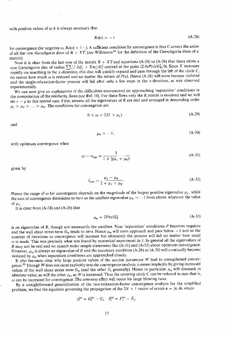
with positive values of co it is always necessary that

Re(v) > - 1 (A-28)

for convergence (for negative co, Re(v) < 1 - ) . A sufficient condition for convergence is that C covers the union of all the row Gerschgorin discs of R + XT. (see Wilkinson z6 for the definition of the Gerschgorin discs of a

matrix). Now it is clear from the last row of the matrix R + X T a n d equations (A-24) to (A-26) that there exists a

row Gerschgorin disc of radius ~ - 1 ~Ss[l~ + X m y G 2 centred at the point (2 6sP(x)/G~, 0). Since X increases rapidly on marching in the x-direction, this disc will quickly expand and pass through the left of the circle C, no matter how much co is reduced and no matter the nature of P(x). Hence (A-28) will soon become violated and the single-relaxation-factor process will fail after only a few steps in the x-direction, as was observed

experimentally. We can now give an explanation of the difficulties encountered on approaching 'separat ion ' conditions in

the computat ion of the similarity flows (see Ref. I0). For these flows only the R matrix is involved and we will set v = # in this special case. First, assume all the eigenvalues of R are real and arranged in descending order #1 > #2 > . . . > #N. The conditions for convergence are

0 < co < 2/(1 + #1) (A-29)

and

#N > - 1, (A-30)

with opt imum convergence when

1 (A-31) co = coop, = 1 + ½(#x + #~)

given by

#1 - #N (A-32) " ~ m i n - - 2 + #1 + #N"

Hence the range of co for convergence depends on the magnitude of the largest positive eigenvalue #1, while the rate of convergence diminishes to zero as the smallest eigenvalue #N ~ - 1 from above, whatever the value

of/z,~. It is clear from (A-24) and (A-26) that

I~,. = 2P6s/G2 (A-33)

is an eigenvalue of R, though not necessarily the smallest. Near 'separat ion ' conditions P becomes negative and the wall shear stress term GN tends to zero. Hence #,, will soon approach and pass below - 1 and so the number of iterations to convergence will increase but ultimately the process will fail no matter how small co is made. This was precisely what was found by numerical experiment in I. In general all the eigenvalues of R may not be real and we cannot make simple statements like (A-31) and (A-32) about opt imum convergence. However, #,, is always an eigenvalue of R and the necessary condition (A-28) or (A-30) will eventually become violated by #m when separation conditions are approached closely.

It also becomes clear why large positive values of the suction parameter W lead to strengthened conver- gence, lo Though Wdoes not enter explicitly into the convergence analysis, it enters implicitly by giving increased values of the wall shear stress term GN (and the other Gi generally). Hence in particular #,, will diminish in absolute value, as will the other #k, as W is increased. Thus the covering circle C can be reduced in size, that is, co can be increased for convergence. The converse effect will occur for large blowing rates.

By a straightforward generalisati0n of the two-relaxation-factor convergence analysis for the simplified problem, we find the equation governing the propagation of the 2N x 1 vector of errors e = {~, 8), where

~I n~ = Gl n~ - Gi , 61 "I = F! ~ - F i ,

17

is now

e (n+ t) = M~zn)eln),

where M 2 is now the 2N x 2N parti t ioned matrix

(A-34)

m 2 .~ CA CB + D (A-35)

A, B, C and D are the N x N matrices

A = I - c o ( l + R),

C = - ( o ' X diag (1/G 2 . . . . . I/G2),

B = coQ~

D = (1 - ~o')I, (A-36)

with R as defined in (A-24) and Q = (fli~) (see (A-25)).

Now a similarity transform of the form S M S - ~ where S is a non-singular matrix leaves the eigenvalues of M unchanged (see, for example, Wilkinson, 26, p. 6). Choos ing

[; o] [; o] S = C - l ' i . e .S - I = , (A-37)

we find that under this t ransformation the matrix M 2 becomes

M ; - - = BC + D co(l + R) I - co'(l + coXT)J" (A-38)

The point of this t ransformation (as in the simplified problem) is to show how the factors co and co' come to- gether and offset the growth of the factor X.

It is usual in discussing the convergence of linear systems to try to establish a relation between the eigenvalues of the iteration matrix M'2(co, co') and those of a related simpler matrix which is independent of the relaxation factors. This is the underlying idea of the classical S.O.R. methods. Such relations can usually be found only for very restricted classes of matrices (see Young, 27 p. 140). In the present case, the author has not been able to establish any such connect ion on account of the very general nature of the matrices R and T. The most that can be deduced in this direction seems to be the following particular relations :

3 .= 1 - c o ( I + v) c o ' = 1,

and (1 -- co' -- ;t)N(l -- ~l) N = 0 (2) = 0, (A-39)

R - ( 1 - c o - ~ ) I ( l c o - - , ; t ) N = 0 ~O = 0 , '

where the 2. are the non-zero eigenvalues of M) and the v are the eigenvalues of R + XT. The first of these results tells us nothing we do not already know from the single-relaxation-factor process; the last two tell simply that convergence will not occur when either co or co' is zero, 2 = 1 then being a root of multiplicity N. As the iterative process does in fact converge for small positive values of co and co', the matrix M~ must be a convergent matrix for some region of the positive (co, co')-quarter-plane. It may be that there is some qualitative resemblance between this region and the region shown in Figs. 12 and 13 for the simplified problem.

We can, however, easily deduce a relation which determines how closely the separation point can be ap- proached before our iterative process fails to converge. By expanding the determinant [M~ - ,,t12] along the 2Nth column and then the determinant so obtained along its Nth column, we easily see that

2~,, = 1 -co ' ,

2m= 1 -co( l + Vm)= l --CO {l + 2 P ( x ) ~ }

(A-40)

(A-41 )

18

are always eigenvalues of M~. Clearly, co' must always be positive and <2 from (A-40). Also, by (A-41) the necessary condition (A-28) puts the restriction

P(x,) > - ½G~v/6s (A-42)

on the distance x, one can approach the separation point when using positive values of co. For a given flow, the smaller as is made the nearer one can get to separation and this indeed was found to be the case experi- mentally. As noted earlier, the Aitken process enables one to get even closer. It is sometimes possible after (A-42) becomes violated to get a little nearer still by reversing the sign of the relaxation factor for GN (i.e. putting co N = --CON in (A-43) below) for then 12,,I becomes less than unity. This does not constrain all the other eigen- values of M~ to lie inside the unit circle however, and so the device is likely to be of limited usefulness.

We have considered throughout only two scalar relaxation factors co and co'. The analysis generalises readily to case when they are replaced by the matrices

= diag(col . . . . . coN) and f~' = diag(co'l . . . . . co~v), (A-43)

though we lack afortiori some means of prescribing the co, and co', for convergence. For the circle flow, the matrices R and T and the various derived matrices were computed using solution

values for G(s,, x) on a coarse mesh across the boundary layer. With the aid of a subroutine to compute the spectral radius of a general matrix it was verified that the simple iteration scheme (A-18) fails after a few steps in the x-direction. Furthermore, it was verified at several x-stations that the matrix M~(co, co') was convergent for those values of co and co' which had given convergence in the two-field scheme (A-19).

A2. Stability A.2.1. An explicit-type scheme. Suppose we replace the t?(1/G)/Ox terms by the following difference formula

involving function values at two previous x-stations,

x, 1( , 1 ) , ( 1 1) , 44, j, = - ax ) G ( s , , x j - 2ax) = G,;_2

This means when we iterate equation (10) the terms involving the factor X = x/6x are not included in the iteration. This would seem to be a very convenient way of avoiding the difficulties of the large factor X inside the iteration. However, it was found experimentally that this process was unstable for all the (ax, &)-pairs that were tried. We shall see why this is the case from the following local matrix stability analysis.

As the equations are non-linear we first have to linearise them by setting G = G + g where g(s, x) is a small perturbation. We shall again simplify the problem by using the Trapezium rule for the integrals. The set of linear equations which have to be solved to advance the perturbation solution g from the (j - 2)th and ( j - 1)th x-stations to the jth x-station may be written in matrix form as,

gj = - X ( I + Rj)-lTj_lgj_t + X(I + R j ) - l r j _ 2 g j _ 2 , (A-45)

where the matrices R and T are again given by (A-24) and (A-25). This is a three-level formula which can be reduced to a two-level formula by setting

I g J ] = HFgJ - ' - ] , (A-46, hj khj_ 1 J

where

I - X ( I + R ) - I T J - 1 X(I+R;)-IT~-21 (A-47) H = I

is the 2N x 2N amplification matrix (for example, see Mitchell, 15, p. 87). The eigenvalues of H are given

by the roots of the determinantal equation

[/~2(i -t- R j ) - ~ x r j - 1 - x r j - 2 [ -- 0. (A-48)

19

Stability depends on the spectral radius of H being less than unity. It is clear that for fixed 3x and 6s this spectral radius must increase as x increases. In fact, it will soon become greater than unity and render the scheme useless. It is interesting to note that for a fixed value of the step-size 3s, the tendency to instability becomes greater the smaller the step-size 3x in the marching direction--which is the opposite tendency of the standard explicit methods for parabolic equations. It may be that the scheme is stable at any x-station for large enough 6x and/or small enough 6s--i.e. conditionally stable. The appropriate stability criterion is not readily deducible however, from the above analysis. The author is of the opinion that even if it exists it would make rather too stringent demands on the values of 6x and 6s for the scheme to be practicable. In any case, difference formulae of the type (A-44) are not very accurate.

A.2.2. lmplicit scheme. We first replace the O(l/G)/~x-terms by the usual two-point formula:

~x ~si' 6x G(s~ xj) G(s i, xj - bx) = ~x ,j Gi,~- l " (A-49)

On linearising and using the Trapezium rule for the integrals we find the equations that have to be solved to advance the perturbation solution from the (j - 1)th x-station to the jth x-station are

gj = Hgj_ 1,

where the amplification matrix is now the N × N matrix

(A-50)

H = (I + Rj + XTj)-1XTj_I (A-51)

which is clearly of implicit type. One feels intuitively that the spectral radius of H should be less than unity for all X and 6s when Rj + X ~ and XT~ 1 are non-negative matrices--which they are in all the cases con- sidered in this report. Unfortunately, these matrices seem to be of too general a character for the well-known Perron-Frobenius theory to provide a proof that H is a convergent matrix (see Varga, 23, p. 30).

When we use the three-point formula for the x-derivative terms, the amplification matrix becomes

H = [2(I + Rj + ~XTj) - IXTj-1 - ½(I + R~ + ~XTj) - IXTj_2]

1 0 " (A-52)

The crucial implicit nature of the scheme remains in evidence, however. Experimentally, the author found the scheme to be stable for every flow considered and every combination of step sizes.

The discussion of convergence and stability is a little more complicated when we use Simpson's rule and equations (17) and (18) for the x-derivative terms (i.e. differences on G2). However, the general convergence and stability characteristics of the algorithm remain as described above. The author has verified directly the stability characteristics of schemes A.2.1 and A.2.2 for the circle flow by computing the spectral radii of the appropriate amplification matrices at solution using a coarse mesh across the boundary layer.

20

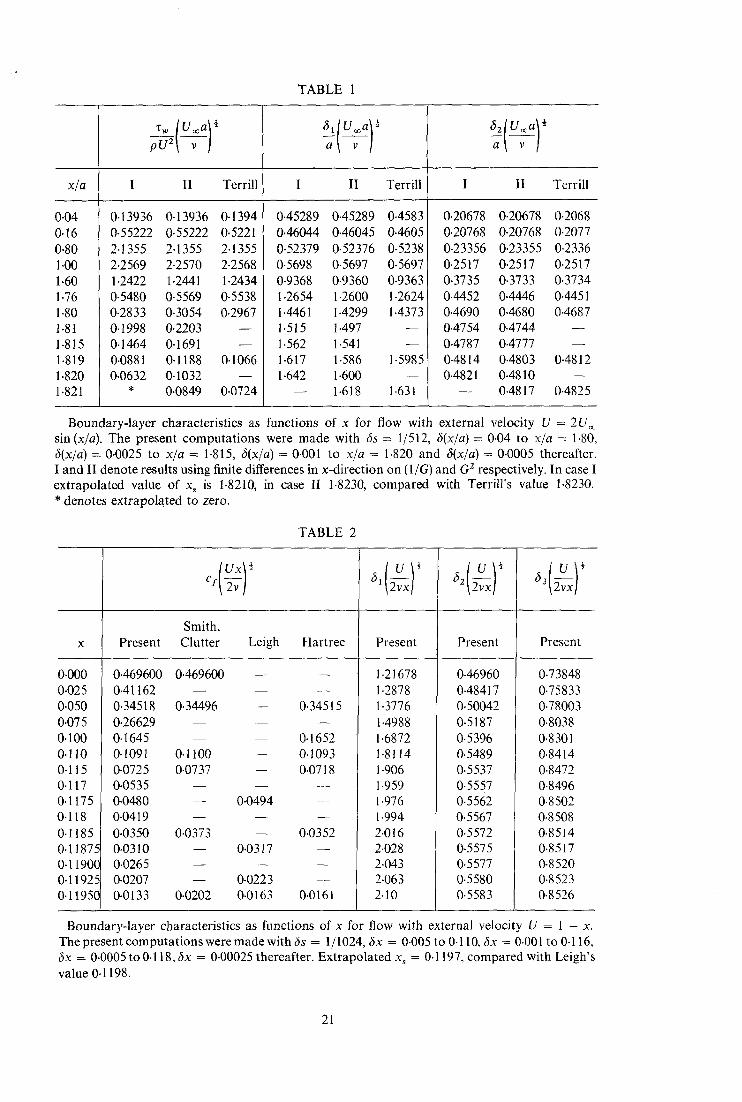
TABLE 1

IV ap or21 v I

~1 'Foo d a v

L i a ~ v l

x/a I II Terrill I II Terrill I II Terrill

0.45289 0.45289 0.4583 0.46044 0.46045 0.4605 0-52379 0.52376 0-5238 0.5698 0.5697 0.5697 0.9368 0.9360 0.9363 1.2654 1.2600 1.2624 1.4461 1 - 4 2 9 9 1-4373 1.515 1.497 1.562 1.541 - - 1-617 1-586 1-5985 1-642 1-600

1.618 1.631

0.13936 0.13936 0.1394 0-55222 0.55222 0.5221 2.1355 2.1355 2.1355 2.2569 2.2570 2-2568 1.2422 1 .2441 1.2434 0-5480 0.5569 0.5538 0.2833 0.3054 0.2967 0.1998 0.2203 0.1464 0.1691 0.0881 0.1188 0.1066 0.0632 0.1032

* 0.0849 0.0724

0.20678 0.20678 0.2068 0.20768 0.20768 0.2077 0-23356 0.23355 0.2336 0.2517 0.2517 0.2517 0.3735 0.3733 0.3734 0-4452 0.4446 0.4451 0.4690 0.4680 0.4687 0.4754 0.4744 0.4787 0.4777 0.4814 0.4803 0.4812 0.4821 0.4810

0.4817 0.4825

3.04 3.16 D.80 1.00 1.60 1.76 1.80 1.81 1.815 1-819 1.820 1.821

Boundary-layer characteristics as functions of x for flow with external velocity U = 2U~o sin (x/a). The present computations were made with 6s = 1/512, 3(x/a) = 0.04 to x/a = 1.80, 6(x/a) = 0.0025 to x/a = 1.815, 6(x/a) = 0-001 to x/a = 1.820 and 6(x/a) = 0-0005 thereafter. I and II denote results using finite differences in x-direction on (l/G) and G 2 respectively. In case I extrapolated value of x~ is 1.8210, in case II 1.8230, compared with Terrill's value 1.8230. * denotes extrapolated to zero.

TABLE 2

0.000 0-025 0.050 0.075 O.lO0 0.110 )-115 3.117 0.1175 ~.118 0.1185 0.11875 0.11900 0-11925 0.11950

[Uxl i

Smith, Present Clutter Leigh Hartree

0.469600 0.41162 0-34518 0.26629 0.1645 0.1091 0-0725 0.0535 0.0480 0.0419 0.0350 0.0310 0.0265 0.0207 0.0133

0.469600 - -

0.34496 - - 0.34515

0-1652 0.1100 0.1093 0-0737 - - 0.0718

0.0494

0-0373 0.0352 0.0317

0.0223 0-0202 0.0163 0.0161

Present

1.21678 1-2878 1-3776 1-4988 1.6872 1-8114 1-906 1.959 1.976 1.994 2.016 2.028 2.043 2.O63 2.10

Present

0.46960 0.48417 0.50042 0.5187 0.5396 0.5489 0.5537 0-5557 0-5562 0.5567 0-5572 0.5575 0.5577 0.558O 0-5583

12vx]

Present

0-73848 0-75833 0.78003 0.8038 0.8301 0-8414 0.8472 0.8496 0.8502 0-8508 0.8514 0.8517 0-8520 0-8523 0.8526

Boundary-layer characteristics as functions of x for flow with external velocity U = 1 - x. The present computations were made with 6s = 1/1024, fix = 0.005 to 0.110, fix = 0.001 to 0.116, 6x = 0.0005 to 0-118, fix = 0.00025 thereafter. Extrapolated x s = 0.1197, compared with Leigh's value 0.1198.

21

b ~

j=O ! i=o !0

I Z 3

N

1,

Z 3 Outer edge

/ o f B.L.

" / / / / / / / / / Wall

. 2 /

r

FIG. 1.

I , ~u.~,½ _~ . I I I I /

3 - 5 3 - N u m e r i c a l V e l o c i t y

/ Analyticol profiles / / ,~q ~ /

/ Rheinboldt at / / # /7 /

I ............ x 7 7 S 7 7 o Smith and Clutter ~ =

U= Scale / /JJ ~ i " " " ,,11 I I I 1 I I 1 1 i . / _.--~ _ _ ~

<'u N 0 0"2 0"4 0"6 0"8 I'0 ...~.~..--'~ / ~ / ~ " ~

'~ ~ / ~ ) ' ~ - ~

I'0

0"5 ""'" ...

1 I I 1 l l i l i l l l I I I I £ 0 0"2 0"4 0"6 0"8 I'0 I-2 1"4 1"6 1"8 2"0

FIG. 2. Suction step and pulse. Velocity profiles, shear stress distributions and displacement thicknesses for S = -(wo/U®)(UoJ/v) ~ = 1.5.

Blasius

Z.5

2.0

t'O 4~

3.0

2.5

2.0

I ~, (U~o~/~ 7- , -5--,

r ' ,4 -----S = 1.5

6-0

I-5

1.0

).5

1"5

1.0

0.5

I '7" w

~ 6"0

3"0

/ ' 1 ~ ,.5

J 0-2

l__ 0.4

1 /

Blasius x

0.6 0-8 I'0 1-2 1-4 I-6 1.8 2.0

FlG. 3. Suction pulse of varying width with same total suction quantity.

3'0

2"5

2"0

1,5 I

m

s

5 =-0'75

1"5

0"75

1.0

0.5

I

+0-75

1 L 0 0.2 0.4 0.6

-0-75 ;X ] 1 / "E

1.6 I-8 2'0

FIG. 4. Spaced suction and blowing pulses.

b ~

" 2 " 0

- - I - 5

P=O 61 Uo~£

j ,.o

o "' ,o " --j o

_x I I I I t~

0 0"2 0"4 0"6 0"8 I-0 1"2 1"4 1'6 1"8 2" 0

0.5

FIG. 5. Suction pulses in flat plate (P -- 0), 90 ° wedge (P = ½) and stagnat ion flow (P = 1).

t'-O

1"50

1"25

I'00

0'75

0"50

0'Z5

I

c1 (-U-~-) ~"

P = i

I 0 0.5

O Smith and Clutter

I I I I J I 1.0 1.5 2"0 2.5 3-0 3-5

Asymptotes

I I × 4.0 4.5 5.0

FIG. 6. Step change in pressure gradient. Shear stress distribution.

4 '01 -13"0

3 " 5 m

3 " 0 -

1.5 f

I'0 \ \

I 0 0'2

2.5

2.0

0.5

Blasius

6, uoo~/½

I

eu~

I I I I I I I 0-4 0.6 0"8 I'0 1-2 1"4 1"6

~ . ~ 2.5

- 2.0

-1"5

- O.S

1-8 2"0

I ' 0

FIG. 7. Per iodic suct ion at wall S(x) = S sin (lOzcx/l) for S = 1-0.

4.0[

15.5

3-0

2.5

Blasius

I

E = O'OI

"~-E = 0-02

3-0

2-5

2.0

1"5

h.)

2.0

I-5

I-0

0.5

I-0

0.5

• ~ ( u ~ ½

=o.o2

/ E =0-01

I I I I ~ I I I. 0"2 0-4 0"6 O'B I-0 I'2 1.4 1"6 1"8

0

2'0

FIG. 8. Periodic mainstream u = u~(1 + e sin (5nx//)) for e = 0-01 and 0.02.

I

3-6

.~.0,-

2.4

I.B

1.2

0"6

- F +

+

X

5=I

÷

Tcr r i l l

Watson

o . 4 1 o.~ I ~.z 1~-6 z.o/ z.4 30 o 60 o 900 120 °

~'w

x\x \

Q

I 2.s "%z 150 ° 180 °

FIG. 9. C i rcu la r cy l inde r U = 2 U o~ s in (x/a). S h e a r s t r e s s d i s t r i b u t i o n s . S = - (Wo/U~)(Uooa/v) ~.

I 1"4--

+

x Wa tson

1"2

1.0

0-8

O.

.,

0 " i - -

S:O / 1 \ _ + / - / S : l

5 x x

,/'~/z

x x - x__.__._ X ~ X ~ - X ~

X a

I J I I I I I o.4 I o-8 I 1.2 11.6 Z.Ol 2.4 I z.8 13.z

30 o 60 o 900 I ZO o 1500 ,1800

FIG. 10. Circular cylinder U = 2U~ sin (x/a). Displacement thickness distributions.

I< I I I I

_I

FIG. 11.

0 n

60

Simplified problem. Range of convergence of simple iteration process.

32

Z

4--Z o~ I

i ~ =(F,'~T-~')+Xto 3'

, .

, i

I Z " " " - ~ Z(I+r_____L _} 2

I+r-- Xt I+r-Xt

FIG. 12. Simplified problem. Region of convergence of double-field i terat ion process when x = 1-0, P = 0.64, G = 0.91, r ~ 0.8 and X t ~ 20.

2 o0

(.~1 r sing

~ = ( I + r ) (6o I - I )

£3 I

i z

FIG. 13. Simplified problem. Region of convergence of double-field i terat ion process when x = 2-0, P = - 0.92, G = 0.63, r ~ - 2 . 3 , X t ~ 100.

Printed in England for Her Majesty's Stationery Office by J. W. Arrowsmith Ltd., Bristol BS3 2NT Dd 505715 K5 5/74

33

IR. & M. No. 3742

© ('rown copyright 1974

HER MAJESTY'S STATIONERY OFFI( ' [!

Goi,ernmen! Bookshops

49 High ttolborn, London WCIV 6HB 13a ( 'astle Street. Edinburgh EH2 3AR

4l The Itayes, ( 'ardiff CI:I IJW Brazennosc Street, Manchester M60 8AS

Soulhcy Itouse, Wine Street, Bristol BSI 2BQ 258 Broad Street, t t irmingham BI 2HE 80 Chichester Street+ Belfast BT1 4.1Y

Government publications are aL;o avaih~hh" through booksellers

R. & NI. No. 3742

~SBN 0 I1 470835 5