Embed Size (px)
Citation preview
Boundary Layer Problems in the Viscosity-DiffusionVanishing Limits for the Incompressible MHD Systems
Shu Wanga, Zhouping XinbaCollege of Applied Sciences, Beijing University of Technology, Ping Le Yuan 100
Beijing 100124, P. R. ChinaEmail: [email protected]
b The Institute of Mathematical Sciences, The Chinese University of Hong KongShatin, N. T., Hong Kong
Email: [email protected]
Abstract:In this paper, we we study boundary layer problems for theincompressible MHD systems in the presence of physical boundaries withthe standard Dirichlet boundary conditions with small generic viscosityand diffusion coefficients. We identify a non-trivial class of initial datafor which we can establish the uniform stability of the Prandtl’s typeboundary layers and prove rigorously that the solutions to the viscousand diffusive incompressible MHD systems converges strongly to thesuperposition of the solution to the ideal MHD systems with a Prandtl’stype boundary layer corrector. One of the main difficulties is to deal withthe effect of the difference between viscosity and diffusion coefficientsand to control the singular boundary layers resulting from the Dirichletboundary conditions for both the viscosity and the magnetic fields. Onekey derivation here is that for the class of initial data we identify here,there exist cancelations between the boundary layers of the velocity fieldand that of the magnetic fields so that one can use an elaborate energymethod to take advantage this special structure. In addition, in thecase of fixed positive viscosity, we also establish the stability of diffusiveboundary layer for the magnetic field and convergence of solutions inthe limit of zero magnetic diffusion for general initial data.2000 Mathematics Subject Classification: 35Q30, 35Q35, 35Q40,35Q53, 35Q55, 76D05, 76Y07Keywords: Incompressible viscous and diffusive MHD systems, idealinviscid MHD systems, boundary layer for Dirichlet boundary condi-tions.
1
1 Introduction
We consider in this paper boundary layer problems, zero viscosity-diffusion vanishinginviscid limit and zero magnetic diffusion vanishing limit for the three/two-dimensionalincompressible viscous and diffusive magnetohydrodynamic(MHD) systems with Dirichletboundary (no-slip characteristic) boundary conditions
∂tuε + uε · ∇uε +∇pε − ε1∆uε = bε · ∇bε, in Ω× (0, T ), (1.1)
∂tbε + uε · ∇bε − ε2∆bε = bε · ∇uε, in Ω× (0, T ), (1.2)
divuε = 0, divbε = 0, in Ω× (0, T ), (1.3)
uε = 0, bε = 0, in ∂Ω× (0, T ), (1.4)
uε(t = 0) = uε0, bε(t = 0) = bε0, with divuε0 = divbε0 = 0 on Ω, (1.5)
where Ω = ω × [0, h] or Ω = ω × (0,∞), and ω = T2 or R2 in three dimensional casefor MHD systems, and ω = T1 or R1 in two dimensional case for MHD systems. ∆ =∂2
∂x2+ ∂2
∂y2+ ∂2
∂z2or ∆ = ∂2
∂x2+ ∂2
∂z2is the three-dimensional or two-dimensional Laplace
operator, ε1 = ε1(ε) > 0 is the viscosity coefficient and ε2 = ε2(ε) > 0 is the magneticdiffusion coefficient. The unknown functions uε, pε, bε are the velocity, the pressure andthe magnetic field of MHD.
The well-posedness, regularity and asymptotic limit problem on the incompressibleviscous and diffusive MHD systems (1.1)-(1.3) in the whole space or with slip/no-slipboundary conditions have been studied extensively, see [2, 3, 4, 5, 9, 10, 19, 21, 22, 23, 25]and the references therein. When ε1 > 0 and ε2 > 0, MHD systems in the whole space andin the bounded domains with slip boundary conditions for the velocity and with no-slipboundary condition for the magnetic field has a unique global classical solution for smoothinitial data when space dimension d = 2 and has a global weak solution for a class of initialdata when d = 3, see [5, 19]. Some regularity criterions are also given by some authors,see [3, 4, 9, 21, 22] and therein references. Cao and Wu [3] obtain global regularity for the2D MHD equations with mixed partial dissipation and magnetic diffusion for any smoothinitial data. Wu [21] considers the inviscid limit problem of incompressible viscous MHDsystems in the whole space. Xiao, Xin and Wu [25] investigate the solvability, regularityand vanishing viscosity limit of incompressible viscous MHD systems with slip withoutfriction boundary conditions.
It should be noted that, as in the zero-viscosity vanishing limit for the Navier-Stokesequations, see[1, 3, 6, 7, 8, 11, 12, 13, 14, 15, 16, 17, 18, 20, 26] and related references,the zero-viscosity and diffusion vanishing limit for incompressible viscous and diffusiveMHD system in a bounded domain, with Dirichlet boundary conditions at the boundary,is a challenging problem due to the possible appearance of boundary layers. Recently,[24] considers boundary layer problems and zero viscosity-diffusion vanishing limit of theincompressible MHD system with no-slip boundary conditions and the case ε1 = ε2 or thecase of the the different horizontal and vertical viscosities and magnetic diffusions. In this
2

paper, we consider the boundary layer problems for the more general case ε1 6= ε2 andalso consider the zero magnetic diffusion limit.
Letting ε1 → 0 and ε2 → 0 in (1.1)-(1.5), one obtains formally the following inviscidMHD systems
∂tu0 + u0 · ∇u0 +∇p0 = b0 · ∇b0, in Ω× (0, T ), (1.6)
∂tb0 + u0 · ∇b0 = b0 · ∇u0, in Ω× (0, T ), (1.7)
divu0 = 0, divb0 = 0, in Ω× (0, T ), (1.8)
u0 · n = ±u03 = 0, b0 · n = ±b03 = 0, in ∂Ω× (0, T ), (1.9)
u0(t = 0) = u00, b
0(t = 0) = b00, with divu00 = divb00 = 0 on Ω. (1.10)
On the other hand, setting the magnetic diffusion coefficient ε2 → 0 in (1.1)-(1.5), onegets formally the following viscous MHD systems
∂tuε1,0 + uε1,0 · ∇uε1,0 − ε1∆uε1,0 +∇pε1,0 = bε1,0 · ∇bε1,0, in Ω× (0, T ), (1.11)
∂tbε1,0 + uε1,0 · ∇bε1,0 = bε1,0 · ∇uε1,0, in Ω× (0, T ), (1.12)
divuε1,0 = 0, divbε1,0 = 0, in Ω× (0, T ), (1.13)
uε1,0 = 0, bε1,03 = 0, in ∂Ω× (0, T ), (1.14)
uε1,0(t = 0) = uε1,00 , bε1,0(t = 0) = bε1,00 , with divuε1,00 = divbε1,00 = 0 on Ω.(1.15)
The purpose of this paper is to prove rigorously the above formal limits under some as-sumptions on initial data or viscosity and diffusive coefficients. Since we can recoverthe incompressible Navier-Stokes equations by taking bε = 0 in MHD systems (1.1)-(1.5),and, hence, the basic difficulties caused by such as the well-posedness of the Prandtl’s typeboundary layer equations, the thickness of the boundary layer and nonlocal pressure whendealing with the boundary layer problem and zero viscosity vanishing limit of the incom-pressible NS equations in domains with boundaries are kept here. The key ingredients hereare that we will be able to identify a non-trivial class of initial data for which there existcancelations between boundary layers of the velocity field and that of the magnetic field,which make the stability of the boundary layers and uniform convergence possible. Hencethe method used here can not be extend directly to deal with the boundary layer problemfor incompressible Navier-Stokes equations. Moreover, the zero magnetic diffusion limitfor MHD systems in a domain with the boundary is also non-trivial due to the nonlinearcoupling of the velocity field and the magnetic field. The boundary layer problem for themagnetic field can not also be obtained and it is remained open in general, see Remark2.4.
The paper is organized as follows. In section 2 we give the main results of thispaper. Section 3 is devoted to the proofs of Main results, including the constructs of theapproximating boundary layer functions.
3
2 The main results
In this section, we state our main Theorems. For this, we first recall the following classicalresults on the existence of sufficiently regular solutions to the incompressible ideal MHDsystem (see [5, 19]).
Proposition 2.1 Let (u00, b
00) satisfy u0
0, b00 ∈ Hs(Ω), s > 3
2 + 1, divu00 = divb00 = 0 and
u00 · n|∂Ω = b00 · n|∂Ω = 0. Then there exist 0 < T∗ ≤ ∞, the maximal existence time,
and a unique smooth solution (u0, p0, b0), also denoted by (u0,0, p0,0, b0,0) below, of theincompressible ideal MHD equations (1.6)-(1.10) on [0, T∗) satisfying, for any T < T∗,
sup0≤t≤T
(‖(u0, b0)‖Hs + ‖(∂tu0, ∂tb
0)‖Hs−1(Ω)
)≤ C(T ).
Moreover, if (u00, b
00) satisfies u0
0 = ±b00, then there is a unique smooth solution (u0, p0, b0) ofincompressible inviscid MHD system satisfying u0(x, y, z, t) = ±b0(x, y, z, t) (= u0
0(x, y, z) =±b00(x, y, z)), p0(x, y, z, t) = 0. Also, there exist the smooth solutions to the initial boundaryproblems for three/two dimensional incompressible ideal MHD systems for the smooth ini-tial data, which maybe not belong to Sobolev space Hs in unbounded domain, for example,the shear flow.
Similarly, for the incompressible MHD with the viscosity (1.11)-(1.15), it is easy to getthe following result on the existence of sufficiently regular solutions.
Proposition 2.2 Assume that ε1 > 0 be fixed. Let (uε1,00 , bε1,00 ) satisfy uε1,00 , bε1,00 ∈Hs(Ω), s > 3
2 + 2, divuε1,00 = divbε1,00 = 0. Then there exist 0 < T∗ ≤ ∞, the maxi-mal existence time, and a unique smooth solution (uε1,0, pε1,0, bε1,0) of the incompressibleMHD equations (1.11)-(1.15) on [0, T∗) satisfying, for any T < T∗,
sup0≤t≤T
(‖(uε1,0, bε1,0)‖Hs(Ω) + ‖(∂tuε1,0, ∂tbε1,0)‖Hs−2(Ω)
)+ε1
∫ T
0‖∇uε1,0(x, y, z, t)‖2Hs(Ω)dt ≤ C(T )
for some positive constant C(T ) independent of ε2. Moreover, if bε1,00 |∂Ω = 0, thenbε1,0(x, y, z, t)|∂Ω = 0.
Now we can state the main results of this paper.For the MHD system (1.1)-(1.5), we have the following stability result of Prandtl’s
type boundary layer for a class of special initial data.
Theorem 2.3 (Stability of the Prandtl boundary Layer) Let (u0, p0, b0) be the so-lution to the incompressible ideal MHD system (1.6)-(1.10). Assume that (uε0, b
ε0) strongly
converges in L2(Ω) to (u00, b
00), where u0
0, b00 ∈ Hs(Ω), s > 3
2 +1 satisfies divu00 = divb00 = 0
4
and u00 · n|∂Ω = b00 · n|∂Ω = 0. Assume that u0
0(x, y, z) = b00(x, y, z) or u00(x, y, z) =
−b00(x, y, z). Furthermore, assume that ε, ε1, ε2 satisfy the following convergence:
ε1 + ε2√ε→ 0,
(ε1 − ε2)2
√εε(ε1 + ε2)
→ 0,(ε1 − ε2)2
ε(ε1 + ε2)≤ C minε1, ε2 (2.1)
for some constant C > 0, independent of ε, ε1, ε2, as ε → 0, ε1 → 0, ε2 → 0. Then thereexists a global Leray-Hopf weak solutions (uε, pε, bε) of (1.1)-(1.5) such that
(uε − u0, bε − b0)→ (0, 0) in L∞(0, T ;L2(Ω)) (2.2)
for any T : 0 < T <∞, as viscosity coefficient ε1 → 0 and diffusion coefficient ε2 → 0.Moreover, if
‖(uε0 − u00, b
ε0 − b00)‖2L2(Ω) ≤ Cε
κ, κ > 1, (2.3)
then there exists C(T ), independent of ε, such that, for 0 ≤ t ≤ T <∞,
‖(uε − u0, bε − b0)‖2L2(Ω) ≤ C(T )(εκ−1 + ε21 + ε2
2 +ε1 + ε2√
ε+
(ε1 − ε2)2
ε√ε(ε1 + ε2)
). (2.4)
Furthermore, we have the following stronger L∞ convergence results for the viscous anddiffusive incompressible 2D MHD systems: Assume that ω = T1 and u0
1(x, z = 0) =b01(x, z = 0) = const (for example, the two-dimensional shear flow) and ε1 = ε2 or thatε, ε1, ε2 satisfy suitable relations(stated below). If, for some suitably large κ > 2,
‖(uε0 − u00 − uεB(t = 0), bε0 − b00 − bεB(t = 0))‖2Hs(Ω) ≤ Cε
κ, s > 3, (2.5)
then there exists C(T ), independent of ε, such that, for 0 ≤ t ≤ T <∞,
‖(uε − u0 − uεB, bε − b0 − bεB)‖L∞(Ω×(0,T ) ≤ C(T )√ε if ε1 = ε2 = ε (2.6)
‖(uε − u0 − uεB, bε − b0 − bεB)‖L∞(Ω×(0,T )
≤ C(T )((β1(ε)
minε1, ε2)14 (β2(ε))
14 + (β0(ε))
14 (
β4(ε)
minε1, ε2)14 )→ 0 when ε→ 0.(2.7)
Here uεB, bεB, β0(ε), β1(ε), β2(ε), β4(ε) will be given more precisely in the next section.
Remark 2.1 If ε1 = ε2 or ε1 = ε, ε2 = ε + εα+1 with α > 12 , then the assumption (2.1)
holds. The boundary layers for the velocity field and the magnetic field in Theorem 2.3occurs, which is the standard Prandtl boundary layer and will be given in the followingsection 3.1. The proof in establishing the stability of the Prandtl boundary layer heredepends strongly upon the special structure of the solution (u0, p0, b0) to the inviscid MHDsystem, i.e. u0 = ±b0, which yields to that there exists the cancelation between the Prandtlboundary layer of the velocity and the one of the magnetic field. Also, the proof of Theorem?? in the case ε1 6= ε2 is more complex than that of the special case ε1 = ε2 > 0 discussedin the paper [24], and here we need some new techniques. Of course, if u0
0|∂Ω = ±b00|∂Ω = 0in Theorem 2.3, called well-prepared initial data, then no Prandtl’s type boundary layeroccurs.
5
Remark 2.2 For the shear flow (u0, p0, b0)(z, t) = (u01(z), u0
2(z), 0, 0, b01(z), b02(z), 0) of theincompressible inviscid MHD system, if u0 = ±b0, then the Prandtl boundary layer forviscosity and diffusive MHD system is stable by using Theorem 2.3.
For the incompressible MHD system (1.1)-(1.5), we also have the following result on thezero magnetic diffusion limit when one fix the viscosity coefficient ε1 > 0.
Theorem 2.4 (The Zero Magnetic Diffusion Limit) Let ε1 > 0 be fixed. Let ε =ε2 → 0. Let us assume that (uε0, b
ε0) strongly converges in L2(Ω) to (uε1,00 , bε1,00 ), where
(uε1,00 , bε1,00 ) ∈ Hs(Ω), s > 32 +2. Assume also that (uε1,0, pε1,0, bε1,0) is the smooth solution
to the system (1.11)-(1.15) defined on [0, T∗) with 0 < T∗ ≤ ∞, given by Proposition 2.2.Then there exists global Leray-Hopf weak solutions (uε, pε, bε) of (1.1)-(1.5) such that
(uε, bε)− (uε1,0, bε1,0))→ (0, 0) in L∞(0, T ;L2(Ω)) (2.8)
for any T : 0 < T < T ∗, as ε2 → 0.Moreover, if
‖(uε0 − uε1,00 , bε0 − b
ε1,00 )‖2L2(Ω) ≤ C(
√ε2)1−τ (2.9)
for any given 0 ≤ τ < 1, then there exists C(T ), independent of ε2, such that
‖(uε, bε)− (uε1,0, bε1,0)‖2L2(Ω) ≤ C(T )(√ε2)1−τ . (2.10)
Remark 2.3 This is also one boundary layer problem here. In fact, if bε1,00 |∂Ω 6= 0, thenthere occurs the boundary layer for the magnetic field due to the difference of the boundaryconditions between bε and bε1,0 in the boundary ∂Ω of the domain.
Remark 2.4 When one replaces the viscosity term ε1∆uε by ε1∂2zu
ε in the system (1.1)-(1.5), similar zero magnetic diffusion limit result in Theorem 2.4 as ε2 → 0 holds. Notethat the non-degeneration of the normal direction of the boundary plays a key role inestablishing the stability of the boundary layer. In fact, the zero magnetic diffusion limitof the following MHD system
∂tuε + uε · ∇uε +∇pε = bε · ∇bε, in Ω× (0, T ),
∂tbε + uε · ∇bε − ε2∆bε = bε · ∇uε, in Ω× (0, T ),
divuε = 0, divbε = 0, in Ω× (0, T ),
uε3 = 0, bε = 0, in ∂Ω× (0, T ),
uε(t = 0) = uε0, bε(t = 0) = bε0, with divuε0 = divbε0 = 0 on Ω
or
∂tuε + uε · ∇uε +∇pε − ε1∆x,yu
ε = bε · ∇bε, in Ω× (0, T ),
∂tbε + uε · ∇bε − ε2∆bε = bε · ∇uε, in Ω× (0, T ),
divuε = 0, divbε = 0, in Ω× (0, T ),
uε3 = 0, bε = 0, in ∂Ω× (0, T ),
uε(t = 0) = uε0, bε(t = 0) = bε0, with divuε0 = divbε0 = 0 on Ω
6
is open if bε|∂Ω 6= 0, which yields the appearance of the boundary layer. Here ∆x,y =∂2
∂x2+ ∂2
∂y2and ε2 = ε.
Remark 2.5 One of the main difficulties to establish the zero viscosity and diffusion limitis to deal with the terms related to the boundary layers in the error equations. However,the proof is elementary if there occurs no boundary layers. For example, it is easy to provethat there exists a T > 0, independent of ε, such that the solution (uε, pε, bε) of the system
∂tuε + uε · ∇uε +∇pε − ε1∆uε = bε · ∇bε, in Ω× (0, T ), (2.11)
∂tbε + uε · ∇bε − ε2∆bε = bε · ∇uε, in Ω× (0, T ), (2.12)
divuε = 0, divbε = 0, in Ω× (0, T ), (2.13)
uε = u0, bε = b0, in ∂Ω× (0, T ), (2.14)
uε(t = 0) = uε0, bε(t = 0) = bε0, with divuε0 = divbε0 = 0 on Ω (2.15)
converges to the solution (u0, p0, b0) of the ideal MHD system (1.6)-(1.10) in the interval[0, T ] in some kinds of norm, for example, in L2(Ω), when ε1 → 0 and ε2 → 0. Herethe function (u0, b0) given in the boundary condition (2.14) of the system (2.11)-(2.15) isdetermined by the solution of the ideal MHD system (1.6)-(1.10).
3 The proofs of Theorems 2.3 and 2.4
We will prove Theorems 2.3 and 2.4 when Ω = ω × [0, h] for 0 < h <∞ and ω = T2. Theother cases (for example, when h =∞) are similar. Our proof is based on the asymptoticanalysis with multiple scales and the classical energy method. We will divide the proof intotwo cases. For well-prepared initial data b0|∂Ω = b00|∂Ω = 0 in Theorem 2.3 or bε1,00 |z=0 = 0,there is no boundary layer for the magnetic field, and, hence, there is no boundary layerfor the velocity in the proof of Theorem 2.3 for the case of well-prepared initial datadue to u0
0(x, y, z) = b00(x, y, z). For the general initial data, i.e., b00|∂Ω = u00|∂Ω 6= 0 or
bε1,00 |z=0 6= 0, if one uses energy method to estimate the error function (uε−u0, bε− b0) or(uε − uε1,0, bε − bε1,0), then integrations by parts introduce some terms which are difficultto control, because uε − u0, bε − b0 or bε − bε1,0 do not vanish at the boundary. So, forgeneral initial data, one needs to construct the boundary layer correctors which allow oneto recover zero Dirichlet boundary condition. When 0 < h < ∞, we will construct theleft and right boundary layers respectively. When h = ∞, we will construct only theleft boundary layer by taking the right boundary layer to be zero. Note that there is noboundary layer for the velocity field in the case of Theorem 2.4.
3.1 The construction of the boundary layers
We only construct the boundary layer (uεB, bεB) for the viscous and diffusive MHD system
with ε1 → 0 and ε2 → 0. In the case that ε1 > 0 is a fixed given constant, the structure
7
and its properties of the boundary layer, denoted also by bεB with ε = ε2, are the same asbεB by replacing the function b0 by bε1,0 and ν∗2 = (θε2)1+τ for any 0 ≤ τ < 1 and for θ > 0sufficiently small.
Because the velocity uε and the magnetic field bε satisfy respectively the zero Dirichletboundary condition at the boundary z = 0, h, but u0|z=0,h 6= 0 and b0|z=0,h 6= 0, we needrespectively construct the correctors for u0 and b0 so as to recover the zero Dirichletboundary condition for the error functions.
Now, we introduce the following exact boundary layers for the velocity field u0:
uεB = uεB+ + uεB−, (3.1)
uεB+ =
U εB+
uε3
=
uε1
uε2
uε3
=
−u0
1(x, y, 0, t)e− z√
ν∗1 (ρ1(z)− ρ′1(z)√ν∗1)− u0
1(x, y, 0, t)ρ′1(z)√ν∗1
−u02(x, y, 0, t)e
− z√ν∗1 (ρ1(z)− ρ′1(z)
√ν∗1)− u0
2(x, y, 0, t)ρ′1(z)√ν∗1√
ν∗1∂zu03(x, y, 0, t)ρ1(z)(e
− z√ν∗1 − 1)
(3.2)
and
uεB− =
U εB−uε3
=
uε1
uε2
uε3
=
−u0
1(x, y, h, t)e− h−z√
ν∗1 (ρ2(z) + ρ′2(z)√ν∗1) + u0
1(x, y, h, t)ρ′2(z)√ν∗1
−u02(x, y, h, t)e
− h−z√ν∗1 (ρ2(z) + ρ′2(z)
√ν∗1) + u0
2(x, y, h, t)ρ′2(z)√ν∗1
−√ν∗1∂zu
03(x, y, h, t)ρ2(z)(e
− h−z√ν∗1 − 1)
(3.3)
where ρ1(z) and ρ2(z) satisfy
ρ1(0) = 1, ρ′1(0) = ρ′′1(0) = 0; ρ1(z) ≡ 0 for z ≥ h
4; 0 ≤ ρ1(z) ≤ 1 for z ∈ [0, h] (3.4)
and
ρ2(h) = 1, ρ′(h) = ρ′′2(h) = 0; ρ2(z) ≡ 0 for z ≤ 3
4h; 0 ≤ ρ2(z) ≤ 1 for z ∈ [0, h]. (3.5)
8
Here uεB+ and uεB− are the left boundary layer at z = 0 and the right boundary layer atz = h for u0 respectively. When h =∞, we can take uεB− = 0.
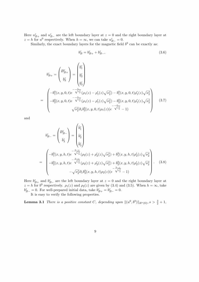
Similarly, the exact boundary layers for the magnetic field b0 can be exactly as:
bεB = bεB+ + bεB−, (3.6)
bεB+ =
BεB+
bε3
=
bε1
bε2
bε3
=
−b01(x, y, 0, t)e
− z√ν∗2 (ρ1(z)− ρ′1(z)
√ν∗2)− b01(x, y, 0, t)ρ′1(z)
√ν∗2
−b02(x, y, 0, t)e− z√
ν∗2 (ρ1(z)− ρ′1(z)√ν∗2)− b02(x, y, 0, t)ρ′1(z)
√ν∗2√
ν∗2∂zb03(x, y, 0, t)ρ1(z)(e
− z√ν∗2 − 1)
(3.7)
and
bεB− =
BεB−
bε3
=
bε1
bε2
bε3
=
−b01(x, y, h, t)e
− h−z√ν∗2 (ρ2(z) + ρ′2(z)
√ν∗2) + b01(x, y, h, t)ρ′2(z)
√ν∗2
−b02(x, y, h, t)e− h−z√
ν∗2 (ρ2(z) + ρ′2(z)√ν∗2) + b02(x, y, h, t)ρ′2(z)
√ν∗2
−√ν∗2∂zb
03(x, y, h, t)ρ2(z)(e
− h−z√ν∗2 − 1)
. (3.8)
Here bεB+ and bεB− are the left boundary layer at z = 0 and the right boundary layer atz = h for b0 respectively. ρ1(z) and ρ2(z) are given by (3.4) and (3.5). When h =∞, takebεB− = 0. For well-prepared initial data, take bεB+ = bεB− = 0.
It is easy to verify the following properties.
Lemma 3.1 There is a positive constant C, depending upon ‖(u0, b0)‖Hs(Ω), s >32 + 1,
9
but independent of ε, ε1 and ε2, such that
‖(uεB, bεB)‖L∞(Ω) ≤ C; ‖(∂zuεB3, ∂zbεB3)‖L∞(Ω) ≤ C;
‖(U εB,∇x,yU εB)‖L2(Ω) ≤ C√√
ν∗1 ; ‖(BεB,∇x,yBε
B)‖L2(Ω) ≤ C√√
ν∗2 ;
‖uεB3‖L2(Ω) ≤ C√ν∗1 ; ‖bεB3‖L2(Ω) ≤ C
√ν∗2 ;
‖∂zU εB‖L2(Ω) ≤C√√ν∗1
; ‖∂zBεB‖L2(Ω) ≤
C√√ν∗2
‖∂zuεB3‖L2(Ω) ≤ C√√
ν∗1 ; ‖∂zbεB3‖L2(Ω) ≤ C√√
ν∗2 ;
‖(z∂zU εB+, (h− z)∂zU εB−)‖L2(Ω) ≤ C√√
ν∗1 ; ‖(z∂zBεB+, (h− z)∂zBε
B−)‖L2(Ω) ≤ C√√
ν∗2 ;
‖(z2∂zUεB+, (h− z)2∂zU
εB−‖L∞(Ω) ≤ C
√ν∗1 ; ‖(z2∂zB
εB+, z
2∂zBεB−)‖L∞(Ω) ≤ C
√ν∗2 ;
ν∗1 , ν∗2 will be chosen later. Here and in what follows we use U,B,UB, BB, UR, · · · or
u1,2, b1,2, uB1,2, bB1,2,uR1,2, · · · to denote the first and the second components ofu, b, uB, bB, uR, · · · respectively. Also, u3, b3, uB3, bB3, · · · , denote the third componentsof the vectors u, b, uB, bB, · · · .
3.2 The proof of Theorem 2.3
The global existence of Leray-Hopf weak solutions to the three dimensional dissipativeincompressible MHD system and the global existence of smooth solutions to the twodimensional dissipative MHD system can be proven as in [5, 19, 25] by Galerkin method,and also as for Navier-Stokes equations. We omit details here.
Let (uε, bε) be Leray-Hopf weak solution of MHD system (1.1)-(1.5). Decompose(uε, bε) as (u0 + uεB + uεR, b
0 + bεB + bεR). Taking ν∗1 = ν∗2 = ε in the subsection 3.1 andusing the system (1.6)-(1.10), we have
∂tuεB + ∂tu
εR + uε · ∇uεR + u0 · ∇uεB + uεB · ∇uεB + uεR · ∇uεB + uεB · ∇u0
+uεR · ∇u0 − ε1∂2zu
εR − ε1∂
2zu
0 − ε1∂2zu
εB − ε1∆x,yu
εR − ε1∆x,yu
0 − ε1∆x,yuεB
= −∇(pε − p0) + bε · ∇bεR + b0 · ∇bεB + bεB · ∇bεB + bεR · ∇bεB+bεB · ∇b0 + bεR · ∇b0, in Ω× (0, T ), (3.9)
∂tbεB + ∂tb
εR + uε · ∇bεR + u0 · ∇bεB + uεB · ∇bεB + uεR · ∇bεB + uεB · ∇b0
+uεR · ∇b0 − ε2∂2zbεR − ε2∂
2zb
0 − ε2∂2zbεB − ε2∆x,yb
εR − ε2∆x,yb
0 − ε2∆x,ybεB
= bε · ∇uεR + b0 · ∇uεB + bεB · ∇uεB + bεR · ∇uεB + bεB · ∇u0
+bεR · ∇u0, in Ω× (0, T ), (3.10)
divuε = divbε = divuεR = divbεR = 0, in Ω× (0, T ), (3.11)
uεR = bεR = 0, on (x, y) ∈ ω, z = 0, h, 0 ≤ t ≤ T (3.12)
uεR(t = 0) = uε(0)− u0(0)− uεB(t = 0),
bεR(t = 0) = bε(0)− b0(0)− bεB(t = 0), on Ω. (3.13)
10
Thanks to the fact that u00 = ±b00, where (u0, p0, b0)(x, y, z, t) = (u0
0, 0, b00) is the special
solution to the incompressible MHD equation, we have that uεB = ±bεB, which shows thatthere exist cancelations between the boundary layers of the velocity and the magneticfield, and, hence, it follows from (3.9) and (3.10) that
∂t(uεR − bεR) + uε · ∇(uεR − bεR)− ε1 + ε2
2∆(uεR − bεR)− ε1 − ε2
2∆(uεR + bεR)
= −∇(pε − p0)− bε · ∇(uεR − bεR) +ε1 − ε2
2∆(uεB + bεB) +
ε1 − ε2
2∆(u0 + b0)(3.14)
or
∂t(uεR + bεR) + uε · ∇(uεR + bεR)− ε1 + ε2
2∆(uεR + bεR)− ε1 − ε2
2∆(uεR − bεR)
= −∇(pε − p0) + bε · ∇(uεR + bεR) +ε1 − ε2
2∆(uεB − bεB) +
ε1 − ε2
2∆(u0 − b0)(3.15)
Here we has used the relation ε1∆uεR − ε2∆bεR = ε1+ε22 ∆(uεR − bεR) + ε1−ε2
2 ∆(uεR + bεR) orε1∆uεR + ε2∆bεR = ε1+ε2
2 ∆(uεR + bεR) + ε1−ε22 ∆(uεR − bεR). Noting that there appears the
term − ε1−ε22 ∆(uεR + bεR) in the system (3.14) due to the fact that ε1 6= ε2, and, hence,
one can not adopt the techniques in [24] here, so a new idea is needed to deal with thecurrent case. Now, using (3.11)-(3.12) and taking the scalar product of (3.14) (or (3.15))with uεR − bεR (or uεR + bεR), we get, for the case of u0 = b0, that
1
2
d
dt
∫|uεR − bεR|2 +
ε1 + ε2
2
∫|∇(uεR − bεR)|2
= −ε1 − ε2
2
∫∇((uεR + bεR) + (uεB + bεB) + (u0 + b0)) · ∇(uεR − bεR) (3.16)
and for the case of u0 = −b0, that
1
2
d
dt
∫|uεR + bεR|2 +
ε1 + ε2
2
∫|∇(uεR + bεR)|2
= −ε1 − ε2
2
∫∇((uεR − bεR) + (uεB − bεB) + (u0 − b0)) · ∇(uεR + bεR), (3.17)
which yields to, by using (3.13) and the properties of the boundary layer functions andwith the help of the Young’s inequality and the assumption (2.3) on initial data, that, for0 ≤ t ≤ T <∞,∫
|(uεR − bεR)(t)|2 + (1− δ)(ε1 + ε2)
∫ t
0
∫|∇(uεR − bεR)|2
≤∫|(uεR − bεR)(t = 0)|2 +
(ε1 − ε2)2
4δ(ε1 + ε2)[
∫ t
0
∫(|∇uεR|2 + |∇bεR|2) + Ct+
C√εt]
≤ Cεκ +(ε1 − ε2)2
4δ(ε1 + ε2)
∫ t
0
∫(|∇uεR|2 + |∇bεR|2) + C
(ε1 − ε2)2
4δ√ε(ε1 + ε2)
(3.18)
11
or ∫|(uεR + bεR)(t)|2 + (1− δ)(ε1 + ε2)
∫ t
0
∫|∇(uεR + bεR)|2
≤ Cεκ +(ε1 − ε2)2
4δ(ε1 + ε2)
∫ t
0
∫(|∇uεR|2 + |∇bεR|2) + C
(ε1 − ε2)2
4δ√ε(ε1 + ε2)
(3.19)
for some constant C > 0 and δ > 0 independent of ε, ε1, ε2, and κ > 1 .Now, by taking the scalar product of (3.14) with uεR and the scalar product of (3.15)
with bεR, one can get that
1
2
d
dt
∫(|uεR|2 + |bεR|2) + ε1
∫|∇uεR|2 + ε2
∫|∇bεR|2 =
13∑i=1
Ji, (3.20)
where Ji, i = 1, · · · , 13, are given respectively as follows
J1 = −∫∇(pε − p0)uεR;
J2 = −∫∂tu
εBu
εR −
∫∂tb
εBb
εR;
J3 = −∫uε · ∇uεRuεR −
∫uε · ∇bεRbεR;
J4 = −∫u0 · ∇uεBuεR −
∫u0 · ∇bεBbεR +
∫b0 · ∇bεBuεR +
∫b0 · ∇uεBbεR;
J5 = −∫uεB · ∇uεBuεR −
∫uεB · ∇bεBbεR +
∫bεB · ∇bεBuεR +
∫bεB · ∇uεBbεR;
J6 = −∫uεR · ∇uεBuεR −
∫uεR · ∇bεBbεR +
∫bεR · ∇bεBuεR +
∫bεR · ∇uεBbεR
J7 = −∫uεB · ∇u0uεR −
∫uεB · ∇b0bεR +
∫bεB · ∇b0uεR +
∫bεB · ∇u0bεR;
J8 = −∫uεR · ∇u0uεR −
∫uεR · ∇b0bεR +
∫bεR · ∇b0uεR +
∫bεR · ∇u0bεR;
J9 =
∫bε · ∇bεRuεR +
∫bε · ∇uεRbεR;
J10 = ε1
∫∂2zu
εBu
εR + ε2
∫∂2zbεBb
εR; J11 = ε1
∫∂2zu
0uεR + ε2
∫∂2zb
0bεR;
J12 = ε1
∫∆x,yu
εBu
εR + ε2
∫∆x,yb
εBb
εR; J13 = ε1
∫∆x,yu
0uεR + ε2
∫∆x,yb
0bεR.
We now bound each of Ji, i = 1, · · · , 13. In the sequel, C denotes any constant dependingonly upon h. Also, in the following, we just consider the case of u0 = b0 in Theorem 2.3because the case of u0 = −b0 can be treated similarly by using (3.19)
12
1) First, using the fact that u0 = b0, which is independent of the time t, and, hence,uεB = bεB, we get
J2 = J4 = J5 = J7 = 0.
2) Second, direct computation gives
J1 = −∫∇(pε − p0)uεR =
∫(pε − p0)divuεR = 0, (3.21)
J3 = −∫uε · ∇uεRuεR −
∫uε · ∇bεRbεR
=1
2
∫uε · ∇(|uεR|2) +
1
2
∫uε · ∇(|bεR|2) = 0, (3.22)
To estimate the term J6, noting that uεB = bεB one gets by using the estimate (3.18) that
J6 = −∫
(uεR − bεR) · ∇uεB(uεR + bεR)
= −∫
(uεR − bεR)1,2 · ∇x,y(uεB)1,2(uεR + bεR)1,2 −∫
(uεR − bεR)1,2 · ∇x,y(uεB)3(uεR + bεR)3
−∫
(uεR − bεR)3 · ∇z(uεB)1,2(uεR + bεR)1,2 −∫
(uεR − bεR)3 · ∇z(uεB)3(uεR + bεR)3
≤ C
∫(|uεR|2 + |bεR|2) + C
∫ |(uεR − bεR)3|2
ε
≤ C
∫(|uεR|2 + |bεR|2) + Cεκ−1 +
(ε1 − ε2)2
4δε(ε1 + ε2)
∫ t
0
∫(|∇uεR|2 + |∇bεR|2)
+C(ε1 − ε2)2
4δε√ε(ε1 + ε2)
, (3.23)
J8 ≤ 2 max‖∇u0‖L∞ , ‖∇b0‖L∞∫
(|uεR|2 + |bεR|2), (3.24)
J9 =
∫bε · ∇(uεR · bεR) =
∫divbε(uεR · bεR) = 0, (3.25)
J10 = −ε1
∫∂zu
εB∂zu
εR − ε2
∫∂zb
εB∂zb
εR
≤ δε1
∫|∇uεR|2 + δε2
∫|∇bεR|2 +
C(ε1 + ε2)√ε
, (3.26)
J11 + J12 + J13 ≤ C∫
(|uεR|2 + |bεR|2) + C(ε21 + ε2
2). (3.27)
13
Combining (3.20) with (3.21)-(3.27) together and using the assumption (2.1) in Theorem2.3, we have
1
2
d
dt
∫(|uεR|2 + |bεR|2) + (1− δ)ε1
∫|∇uεR|2 + (1− δ)ε2
∫|∇bεR|2
≤ C
∫(|uεR|2 + |bεR|2) +
(ε1 − ε2)2
4δε(ε1 + ε2)
∫ t
0
∫(|∇uεR|2 + |∇bεR|2)
+C(εκ−1 + ε21 + ε2
2 +ε1 + ε2√
ε) + C
(ε1 − ε2)2
4δε√ε(ε1 + ε2)
≤ C[
∫(|uεR|2 + |bεR|2) + ε1
∫ t
0
∫|∇uεR|2 + ε2
∫ t
0
∫|∇bεR|2]
+C(εκ−1 + ε21 + ε2
2 +ε1 + ε2√
ε) + C
(ε1 − ε2)2
4δε√ε(ε1 + ε2)
(3.28)
It follows from (3.28) and by Gronwall’s inequality that∫(|uεR|2 + |bεR|2) ≤ C(εκ−1 + ε2
1 + ε22 +
ε1 + ε2√ε
+(ε1 − ε2)2
ε√ε(ε1 + ε2)
). (3.29)
Now, combining (3.18) and (3.29), we can get the estimate (2.4) in Theorem 2.3.For L∞ convergence rate, we just consider the case of two-dimensional MHD system.
For the three dimensional case, the regularity problem involved here is open. To completeour Theorem, we need to do higher order energy estimates. Of course, even though thebasic ideas of doing the higher order energy estimates are the same as in L2 estimates, butthis is very complex. In the following, we just consider the case u0 = b0 and 0 < z < ∞.The others are similar. First, to establish the convergence rate of high order derivatives, weneed solve the exact Prandtl’s type equations so as to obtain the more better convergencerate on the error functions. Second, limited to the length of paper, we just give estimatesof some key terms which will appear when differentiating nonlinear terms of MHD systemand which are required to obtain the estimates by using some kinds of different techniquesfrom the previous steps.
Let the boundary functions uεB(x, z, t) = (uε1B, uε3B) and bεB(x, z, t) = (bε1B, b
ε3B) satisfy
respectively the following Prandtl’s type equations
∂tuε1B = ε∂2
zuε1B
∂1uε1B + ∂3u
ε3B = 0
uε1B(x, z = 0, t) = −u01(x, z = 0), uε1B(x, z =∞, t) = 0
and
∂tbε1B = ε∂2
zbε1B
∂1bε1B + ∂3b
ε3B = 0
bε1B(x, z = 0, t) = −b01(x, z = 0), bε1B(x, z =∞, t) = 0,
14
which can be solved as
uε1B(x, z, t) = −u01(x, z = 0)
∫ ∞z√
ε(t+s)
e−ξ2/4
√π
dξ
bε1B(x, z, t) = −b01(x, z = 0)
∫ ∞z√
ε(t+s)
e−ξ2/4
√π
dξ
for any given constant s > 0 independent of ε. It is easy to verify that, due to the factthat u0
1(x, z = 0) = b01(x, z = 0) = const,
∂tuε3B − ε∂2
zuε3B = 0, ∂tb
ε3B − ε∂2
zbε3B = 0
and the boundary functions uεB, bεB have the similar properties as given in Lemma 3.1.
When u0 = b0, uεB = bεB.Now, replacing (uε, bε) by (u0 +uεB +uεR, b
0 + bεB + bεR) in the MHD system (1.1)-(1.5)and using the system (1.6)-(1.10) in the two-dimensional case, we gets that
∂tuεR + uε · ∇uεR + uεR · ∇uεB + uεR · ∇u0 − ε1∆uεR − ε1∆u0 − (ε1 − ε)∂2
zuεB
= −∇(pε − p0) + bε · ∇bεR + bεR · ∇bεB + bεR · ∇b0, in Ω× (0, T ), (3.30)
∂tbεR + uε · ∇bεR + uεR · ∇bεB + uεR · ∇b0 − ε2∆bεR − ε2∆b0 − (ε2 − ε)∂2
zbεB
= bε · ∇uεR + bεR · ∇uεB + bεR · ∇b0, in Ω× (0, T ), (3.31)
divuε = divbε = divuεR = divbεR = 0, in Ω× (0, T ), (3.32)
uεR = bεR = 0, on x ∈ ω, z = 0, 0 ≤ t ≤ T (3.33)
uεR(t = 0) = uε(0)− u0(0)− uεB(t = 0),
bεR(t = 0) = bε(0)− b0(0)− bεB(t = 0), on Ω. (3.34)
As before, (3.30) and (3.31) imply that
∂t(uεR − bεR) + uε · ∇(uεR − bεR)− ε1 + ε2
2∆(uεR − bεR)− ε1 − ε2
2∆(uεR + bεR)
= −∇(pε − p0)− bε · ∇(uεR − bεR) +ε1 − ε2
2∆(uεB + bεB) +
ε1 − ε2
2∆(u0 + b0)(3.35)
Now, using (3.32)-(3.33) and taking the scalar product of (3.35) with uεR − bεR, yield that
1
2
d
dt
∫|uεR − bεR|2 +
ε1 + ε2
2
∫|∇(uεR − bεR)|2
= −ε1 − ε2
2
∫∇((uεR + bεR) + (uεB + bεB) + (u0 + b0)) · ∇(uεR − bεR), (3.36)
which imply, by using (3.34) and the properties of the boundary layer functions and withthe help of the Young’s inequality and the assumption (2.5) on initial data, that, for
15
0 ≤ t ≤ T <∞,∫|(uεR − bεR)(t)|2 + (1− δ)(ε1 + ε2)
∫ t
0
∫|∇(uεR − bεR)|2
≤∫|(uεR − bεR)(t = 0)|2 +
(ε1 − ε2)2
4δ(ε1 + ε2)[
∫ t
0
∫(|∇uεR|2 + |∇bεR|2) + Ct+
C√εt]
≤ Cεκ +(ε1 − ε2)2
4δ(ε1 + ε2)
∫ t
0
∫(|∇uεR|2 + |∇bεR|2) + C
(ε1 − ε2)2
4δ√ε(ε1 + ε2)
(3.37)
for some constant C > 0 and δ > 0 independent of ε, ε1, ε2, and κ > 2 .Now, by taking the scalar product of (3.30) with uεR and the scalar product of (3.31)
with bεR, we arrive at
1
2
d
dt
∫(|uεR|2 + |bεR|2) + ε1
∫|∇uεR|2 + ε2
∫|∇bεR|2 =
7∑i=1
Ki, (3.38)
where Ki, i = 1, · · · , 7, are given respectively as follows
K1 = −∫∇(pε − p0)uεR;
K2 = −∫uε · ∇uεRuεR −
∫uε · ∇bεRbεR;
K3 = −∫uεR · ∇uεBuεR −
∫uεR · ∇bεBbεR +
∫bεR · ∇bεBuεR +
∫bεR · ∇uεBbεR
K4 = −∫uεR · ∇u0uεR −
∫uεR · ∇b0bεR +
∫bεR · ∇b0uεR +
∫bεR · ∇u0bεR;
K5 =
∫bε · ∇bεRuεR +
∫bε · ∇uεRbεR;
K6 = ε1
∫∂2zu
0uεR + ε2
∫∂2zb
0bεR; K7 = (ε1 − ε)∫∂2zu
εBu
εR + (ε2 − ε)
∫∂2zbεBb
εR.
We now bound each of Ki, i = 1, · · · , 7.1) First, Ki, i = 1, · · · , 6 can be estimated as before for J1, J3, J6, J8, J9.2) Second, we compute
K7 = −(ε1 − ε)∫∂zu
εB∂zu
εR − (ε2 − ε)
∫∂zb
εB∂zb
εR
≤ δε1
∫|∇uεR|2 + δε2
∫|∇bεR|2 + C(
(ε1 − ε)2
ε1√ε
+(ε2 − ε)2
ε2√ε
), (3.39)
Combining (3.38) with (3.21)-(3.25) for Ki, i = 1, · · · , 6 and (3.39) together and using the
16
assumptions (2.1) in Theorem 2.3, we have
1
2
d
dt
∫(|uεR|2 + |bεR|2) + (1− δ)ε1
∫|∇uεR|2 + (1− δ)ε2
∫|∇bεR|2
≤ C
∫(|uεR|2 + |bεR|2) +
(ε1 − ε2)2
4δε(ε1 + ε2)
∫ t
0
∫(|∇uεR|2 + |∇bεR|2)
+C(εκ−1 + ε21 + ε2
2 +(ε1 − ε)2
ε1√ε
+(ε2 − ε)2
ε2√ε
) + C(ε1 − ε2)2
4δε√ε(ε1 + ε2)
≤ C[
∫(|uεR|2 + |bεR|2) + ε1
∫ t
0
∫|∇uεR|2 + ε2
∫ t
0
∫|∇bεR|2]
+C(εκ−1 + ε21 + ε2
2 +(ε1 − ε)2
ε1√ε
+(ε2 − ε)2
ε2√ε
) + C(ε1 − ε2)2
4δε√ε(ε1 + ε2)
. (3.40)
It follows from (3.40) and by Gronwall’s inequality that∫(|uεR|2 + |bεR|2) + ε1
∫ t
0
∫|∇uεR|2 + ε2
∫ t
0
∫|∇bεR|2 ≤ Cβ0(ε). (3.41)
Here
β0(ε) = εκ−1 + ε21 + ε2
2 +(ε1 − ε)2
ε1√ε
+(ε2 − ε)2
ε2√ε
+(ε1 − ε2)2
ε√ε(ε1 + ε2)
. (3.42)
Then we have ∫|(uεR − bεR)(t)|2 + (1− δ)(ε1 + ε2)
∫ t
0
∫|∇(uεR − bεR)|2
≤ C(ε1 − ε2)2
(ε1 + ε2) minε1, ε2β0(ε) + Cεκ + C
(ε1 − ε2)2
√ε(ε1 + ε2)
= β0(ε) (3.43)
Differentiate the equation (3.35) in time, multiply the resulting one by ∂t(uεR − bεR) and
integrate over Ω. Notice that ∂tuεR|t=0 = ε1∆u0(t = 0) +O(εκ + ε1ε
κ + ε1−εε ), ∂tb
εR|t=0 =
17
ε2∆b0(t = 0) +O(εκ + ε2εκ + ε2−ε
ε ) and
|∫∂t(u
ε + bε) · ∇(uεR − bεR) · ∂t(uεR − bεR)|
≤ |∫∂t(u
εR + bεR) · ∇(uεR − bεR) · ∂t(uεR − bεR)|
+|∫∂t(u
0 + b0 + uεB + bεB) · ∇(uεR − bεR) · ∂t(uεR − bεR)|
≤ ‖∇(uεR − bεR)‖L2‖∂t(uεR + bεR)∂t(uεR − bεR)‖L2 + C‖∇(uεR − bεR)‖L2‖∂t(uεR − bεR)‖L2
≤ ‖∇(uεR − bεR)‖L2(‖∂t(uεR + bεR)‖2L4 + ‖∂t(uεR − bεR)‖2L4)
+C‖∇(uεR − bεR)‖L2‖∂t(uεR − bεR)‖L2
≤ ‖∇(uεR − bεR)‖L2(‖∂t(uεR + bεR)‖L2‖∇∂t(uεR + bεR)‖L2 + ‖∂t(uεR − bεR)‖L2‖∇∂t(uεR − bεR)‖L2)
+C‖∇(uεR − bεR)‖2L2 + C‖∂t(uεR − bεR)‖2L2
≤ δ(ε1 + ε2)‖∇∂t(uεR − bεR)‖2L2 + δε2‖∂t∇(uεR + bεR)‖2L2
+C1
ε1 + ε2‖∇(uεR − bεR)‖2L2‖∂t(uεR − bεR)‖2L2 + C
1
ε2‖∇(uεR − bεR)‖2L2‖∂t(uεR + bεR)‖2L2
+C‖∇(uεR − bεR)‖2L2 + C‖∂t(uεR − bεR)‖2L2
Hence we have
d
dt
∫|∂t(uεR − bεR)(t)|2 + (1− δ)(ε1 + ε2)
∫|∂t∇(uεR − bεR)|2
≤ C1
ε1 + ε2‖∇(uεR − bεR)‖2L2‖∂t(uεR − bεR)‖2L2
+C1
ε2‖∇(uεR − bεR)‖2L2‖∂t(uεR + bεR)‖2L2
+C‖∇(uεR − bεR)‖2L2 + C‖∂t(uεR − bεR)‖2L2
+C((ε1 − ε2)2
4δ(ε1 + ε2)+ δε2)
∫(|∂t∇uεR|2 + |∂t∇bεR|2) + C
(ε1 − ε2)2
4δ√ε(ε1 + ε2)
(3.44)
or ∫|∂t(uεR − bεR)(t)|2 + (1− δ)(ε1 + ε2)
∫ t
0
∫|∂t∇(uεR − bεR)|2
≤ C
∫ t
0
‖∇(uεR − bεR)‖2L2
ε2‖∂t(uεR + bεR)‖2L2 + C
(ε1 − ε2)2
(ε1 + ε2)2 minε1, ε2β0(ε)
+Cεκ
ε1 + ε2+ C
(ε1 − ε2)2
√ε(ε1 + ε2)2
+ C(ε1 − ε2)2
+(C(ε1 − ε2)2
4δ(ε1 + ε2)+ δε2)
∫ t
0
∫(|∂t∇uεR|2 + |∂t∇bεR|2) + C
(ε1 − ε2)2
4δ√ε(ε1 + ε2)
(3.45)
for some δ > 0 independent of ε. Here we require β0(ε)minε1,ε2(ε1+ε2) ≤ C.
18
Differentiate the equations (3.30) and (3.31) in time, multiply the resulting ones re-spectively by ∂tu
εR and ∂tb
εR and integrate over Ω. Notice that
|∫
(−∂tuε · ∇uεR∂tuεR + ∂tbε · ∇bεR∂tuεR − ∂tuε · ∇bεR∂tbεR + ∂tb
ε · ∇uεR∂tbεR)|
≤ |∫
(−∂tuεR · ∇uεR∂tuεR + ∂tbεR · ∇bεR∂tuεR − ∂tuεR · ∇bεR∂tbεR + ∂tb
εR · ∇uεR∂tbεR)|
+|∫
(−∂t(u0 + uεB) · ∇uεR∂tuεR + ∂t(b0 + bεB) · ∇bεR∂tuεR
−∂t(u0 + uεB) · ∇bεR∂tbεR + ∂t(b0 + bεB) · ∇uεR∂tbεR)|
≤ C‖∇uεR‖L2(‖∂tuεR‖2L4 + ‖∂tbεR‖2L4) + C‖∇bεR‖L2‖∂tuεR‖2L4 + ‖∂tbεR‖2L4
+C(‖∇uεR‖2L2 + ‖∇bεR‖2L2) + C‖∂tuεR‖2L2 + C‖∂tbεR‖2L2
≤ C(‖∇uεR‖L2 + ‖∇bεR‖L2)(‖∂tuεR‖L2‖∇∂tuεR‖L2 + ‖∂tbεR‖L2‖∇∂tbεR‖L2)
+C(‖∇uεR‖2L2 + ‖∇bεR‖2L2) + C‖∂tuεR‖2L2 + C‖∂tbεR‖2L2
≤ δε1‖∇∂tuεR‖2L2 + C‖∇uεR‖2L2
ε1‖∂tuεR‖2L2 + δε2‖∇∂tbεR‖2L2 + C
‖∇uεR‖2L2
ε2‖∂tbεR‖2L2
+C‖∇bεR‖2L2
ε2‖∂tbεR‖2L2 + C
‖∇bεR‖2L2
ε1‖∂tuεR‖2L2
+C(‖∇uεR‖2L2 + ‖∇bεR‖2L2 + ‖∂tuεR‖2L2 + ‖∂tbεR‖2L2). (3.46)
|∫
(−∂tuεR · ∇uεB∂tuεR + ∂tbεR · ∇bεB∂tuεR − ∂tuεR∇bεB∂tbεR + ∂tb
εR · ∇uεB∂tbεR|
= | −∫∂t(u
εR − bεR) · ∇uεB · ∂t(uεR + bεR)|
≤ C
∫(|∂tuεR|2 + |∂tuεR|2) + C
∫ |∂t(uεR − bεR)|2
ε. (3.47)
|∫
(−uεR · ∂t∇uεB∂tuεR + bεR · ∇∂tbεB∂tuεR − uεR∇∂tbεB∂tbεR + bεR · ∇∂tuεB∂tbεR|
= | −∫
(uεR − bεR) · ∇∂tuεB · ∂t(uεR + bεR)|
≤ C
∫(|∂tuεR|2 + |∂tuεR|2) + C
∫ |uεR − bεR|2ε
. (3.48)
19
Hence we have
d
dt
∫(|∂tuεR|2 + |∂tbεR|2) + ε1
∫|∇∂tuεR|2 + ε2
∫|∇∂tbεR|2
≤ C‖∇uεR‖2L2
ε1
∫|∂tuεR|2 + C
‖∇uεR‖2L2
ε2
∫|∂tbεR|2
+C‖∇bεR‖2L2
ε2
∫|∂tbεR|2 + C
‖∇bεR‖2L2
ε1
∫|∂tuεR|2
+C
∫(|∇uεR|2 + |∇bεR|2) + C
∫(|∂tuεR|2 + |∂tbεR|2)
+C
∫(|uεR|2 + |bεR|2) + C
∫ |∂t(uεR − bεR)|2 + |(uεR − bεR)|2
ε
+C((ε1 − ε)2
ε1√ε
+(ε2 − ε)2
ε1√ε
)
≤ C‖∇uεR‖2L2
ε1
∫|∂tuεR|2 + C
‖∇uεR‖2L2
ε2
∫|∂tbεR|2
+C‖∇bεR‖2L2
ε2
∫|∂tbεR|2 + C
‖∇bεR‖2L2
ε1
∫|∂tuεR|2
+C
∫(|∇uεR|2 + |∇bεR|2) + C
∫(|∂tuεR|2 + |∂tbεR|2)
+C
∫(|uεR|2 + |bεR|2) + C
∫ t
0
‖∇(uεR − bεR)‖2L2
ε3
∫(|∂tuεR|2 + |∂tbεR|2)
+C((ε1 − ε2)2
ε(ε1 + ε2)+ δε)
∫ t
0
∫(|∂t∇uεR|2 + |∂t∇bεR|2) + C
(ε1 − ε2)2
ε+ Cεκ−1
+C(ε1 − ε2)2
ε√ε(ε1 + ε2)
+ C(ε1 − ε2)2
ε(ε1 + ε2) minε1, ε2β0(ε) + C(
(ε1 − ε)2
ε1√ε
+(ε2 − ε)2
ε1√ε
)
+C(ε1 − ε2)2
ε(ε1 + ε2)2 minε1, ε2β0(ε) + C
εκ−1
ε1 + ε2
+C(ε1 − ε2)2
ε√ε(ε1 + ε2)2
+ C(ε1 − ε2)2. (3.49)
It follows from Gronwall’s inequality and (3.49), with the help of the estimates (3.41) and(3.43), that∫
(|∂tuεR|2 + |∂tbεR|2) + ε1
∫ t
0
∫|∇∂tuεR|2 + ε2
∫ t
0
∫|∇∂tbεR|2 ≤ Cβ1(ε). (3.50)
20
Here
β1(ε) = ε21 + ε2
2 +(ε1 − ε2)2
ε(ε1 + ε2)2 minε1, ε2β0(ε) +
εκ−1
ε1 + ε2
+(ε1 − ε2)2
ε√ε(ε1 + ε2)2
+ ((ε1 − ε)2
ε1√ε
+(ε2 − ε)2
ε1√ε
). (3.51)
Here we require β0(ε)ε1+ε2)ε3
≤ C.Then it follows from (3.44) and (3.50) that∫
|∂t(uεR − bεR)(t)|2 + (1− δ)(ε1 + ε2)
∫ t
0
∫|∂t∇(uεR − bεR)|2 ≤ Cβ1(ε),
β1(ε) = (ε1 − ε2)2 +(ε1 − ε2)2
(ε1 + ε2) minε1, ε2β1(ε) +
ε2
minε1, ε2β1(ε) +
(ε1 − ε2)2
√ε(ε1 + ε2)
.(3.52)
Similarly, we can obtain the estimates on tangential derivatives as follows:∫(|∂xuεR|2 + |∂xbεR|2) + ε1
∫ t
0
∫|∇∂xuεR|2 + ε2
∫ t
0
∫|∇∂xbεR|2 ≤ Cβ2(ε). (3.53)
Here
β2(ε) =(ε1 − ε2)2
ε(ε1 + ε2)2 minε1, ε2β0(ε) + ε2
1 + ε22 +
εκ−1
ε1 + ε2+
(ε1 − ε2)2
ε√ε(ε1 + ε2)2
. (3.54)
and ∫|∂x(uεR − bεR)(t)|2 + (ε1 + ε2)
∫ t
0
∫|∇∂x(uεR − bεR)|2 ≤ Cβ2(ε), (3.55)
β2(ε) = εκ +(ε1 − ε2)2
(ε1 + ε2) minε1, ε2β2(ε) +
ε2
minε1, ε2β2(ε) +
(ε1 − ε2)2
√ε(ε1 + ε2)
. (3.56)
Here ‖∂x(uεR(t = 0), bεR(t = 0))‖2L2 = O(εκ) and ∂xuεB = ∂xb
εB = 0.
Finally, we apply ∂t∂x to the equations (3.30)-(3.33) and (3.35), multiply the resultingones respectively by ∂t∂xu
εR, ∂t∂xb
εR and ∂t∂x(uεR− bεR), and integrate over Ω. Notice that
‖∂t∂x(uεR(t = 0), bεR(t = 0))‖2L2 = O(εκ), ε1∂t∂x∆u0 = 0 = ε2∂t∂x∆b0 and ∂t∂xuεB =
21
∂t∂xbεB = 0. Also,
|∫∂t∂x(uε + bε) · ∇(uεR − bεR) · ∂t∂x(uεR − bεR)|
= |∫∂t∂x(uεR + bεR) · ∇(uεR − bεR) · ∂t∂x(uεR − bεR)|
≤ ‖∇(uεR − bεR)‖L2‖∂t∂x(uεR + bεR)∂t∂x(uεR − bεR)‖L2
≤ C‖∇(uεR − bεR)‖L2(‖∂t∂x(uεR + bεR)‖2L4 + ‖∂t∂x(uεR − bεR)‖2L4)
≤ C‖∇(uεR − bεR)‖L2(‖∂t∂x(uεR + bεR)‖2L2‖∇∂t∂x(uεR + bεR)‖2L2
+‖∂t∂x(uεR − bεR)‖2L2‖∇∂t∂x(uεR − bεR)‖2L2)
≤ δ(ε1 + ε2)‖∇∂t∂x(uεR − bεR)‖2L2 + δε2‖∇∂t∂x(uεR + bεR)‖2L2
+C‖∇(uεR − bεR)‖2L2
ε1 + ε2‖∂t∂x(uεR − bεR)‖2L2 + C
‖∇(uεR − bεR)‖2L2
ε2‖∇∂t∂x(uεR + bεR)‖2L2(3.57)
and
|∫∂t(u
ε + bε) · ∇∂x(uεR − bεR) · ∂t∂x(uεR − bεR)|
≤ |∫∂t(u
εR + bεR) · ∇∂x(uεR − bεR) · ∂t∂x(uεR − bεR)|
+|∫∂t(u
0 + b0 + uεB + bεB) · ∇∂x(uεR − bεR) · ∂t∂x(uεR − bεR)|
≤ ‖∇∂x(uεR − bεR)‖L2‖∂t(uεR + bεR)∂t∂x(uεR − bεR)‖L2 + C‖∇∂x(uεR − bεR)‖L2‖∂t∂x(uεR − bεR)‖L2
≤ C‖∇∂x(uεR − bεR)‖L2(‖∂t(uεR + bεR)‖2L4 + ‖∂t∂x(uεR − bεR)‖2L4)
+C‖∇∂x(uεR − bεR)‖L2‖∂t∂x(uεR − bεR)‖L2
≤ C‖∇∂x(uεR − bεR)‖L2(‖∂t(uεR + bεR)‖2L2‖∇∂t(uεR + bεR)‖2L2 + ‖∂t∂x(uεR − bεR)‖2L2‖∇∂t∂x(uεR − bεR)‖2L2)
+C‖∇∂x(uεR − bεR)‖L2‖∂t∂x(uεR − bεR)‖L2
≤ δ(ε1 + ε2)‖∇∂t∂x(uεR − bεR)‖2L2 + C‖∇∂x(uεR − bεR)‖2L2
ε1 + ε2‖∂t∂x(uεR − bεR)‖2L2
+δε2‖∇∂t(uεR + bεR)‖2L2 + C‖∇∂x(uεR − bεR)‖2L2
ε2‖∂t(uεR + bεR)‖2L2
+C‖∇∂x(uεR − bεR)‖2L2 + C‖∂t∂x(uεR − bεR)‖2L2 . (3.58)
Similarly,∫∂x(uε+bε)·∇∂t(uεR−bεR)·∂t∂x(uεR−bεR)can be controlled by δ(ε1+ε2)‖∇∂t∂x(uεR−
bεR)‖2L2+δε2‖∇∂x(uεR+bεR)‖2L2+C‖∇∂t(uεR−b
εR)‖2
L2
ε1+ε2‖∂t∂x(uεR−bεR)‖2L2+C
‖∇∂t(uεR−bεR)‖2
L2
ε2‖∂x(uεR+
22
bεR)‖2L2 + C‖∇∂t(uεR − bεR)‖2L2 + C‖∂t∂x(uεR − bεR)‖2L2 . Thus, we have
d
dt
∫|∂t∂x(uεR − bεR)|2 + (1− δ)(ε1 + ε2)
∫|∇∂t∂x(uεR − bεR)|2
≤ C((ε1 − ε2)2
ε1 + ε2+ δε2)
∫(|∇∂t∂xuεR|2 + |∇∂t∂xbεR|2)
+C
∫|∇∂x(uεR − bεR)|2 + C
∫|∇∂t(uεR − bεR)|2 +
∫|∂t∂x(uεR − bεR)|2
+C‖∇∂t(uεR − bεR)‖2L2
ε1 + ε2
∫|∂t∂x(uεR − bεR)|2
+C‖∇∂x(uεR − bεR)‖2L2
ε1 + ε2
∫|∂t∂x(uεR − bεR)|2
+C‖∇∂x(uεR − bεR)‖2L2
ε2
∫|∂t(uεR + bεR)|2
+C‖∇∂t(uεR − bεR)‖2L2
ε2
∫|∂x(uεR + bεR)|2 (3.59)
or ∫|∂t∂x(uεR − bεR)|2 + (1− δ)(ε1 + ε2)
∫ t
0
∫|∇∂t∂x(uεR − bεR)|2
≤ C((ε1 − ε2)2
ε1 + ε2+ δε2)
∫ t
0
∫(|∇∂t∂xuεR|2 + |∇∂t∂xbεR|2) + Cβ3(ε). (3.60)
Here
β3(ε) = εκ +β1(ε)β2(ε) + β2(ε)β1(ε)
ε2(ε1 + ε2). (3.61)
Here we require β1(ε)(ε1+ε2)2
≤ C.On the other hand,
| −∫
(∂x(uεR − bεR) · ∇∂tuεB + ∂t∂x(uεR − bεR) · ∇uεB) · ∂t∂x(uεR + bεR)|
≤ C
∫(|∂t∂xuεR|2 + |∂t∂xbεR|2) + C
∫ |∂x(uεR − bεR)|2 + |∂t∂x(uεR − bεR)|2
ε
≤ C
∫(|∂t∂xuεR|2 + |∂t∂xbεR|2) + C(
(ε1 − ε2)2
ε(ε1 + ε2)+ δε)
∫ t
0
∫(|∇∂t∂xuεR|2 + |∇∂t∂xbεR|2)
+Cβ3(ε)
ε+ Cεκ−1 + C
(ε1 − ε2)2
ε(ε1 + ε2) minε1, ε2β2(ε) + C
(ε1 − ε2)2
ε√ε(ε1 + ε2)
. (3.62)
23
As in (3.57) and (3.58), one can get that∫[−(∂t∂xu
ε · ∇uεR + ∂tuε · ∇∂xuεR + ∂xu
ε · ∇∂tuεR)
+(∂t∂xbε · ∇bεR + ∂tb
ε · ∇∂xbεR + ∂xbε · ∇∂tbεR)] · ∂t∂xuεR
≤ δε1‖∇∂t∂xuεR‖2L2 + C‖∇uεR‖2
ε1‖∂t∂xuεR‖2L2 + C
‖∇∂xuεR‖2
ε1‖∂tuεR‖2L2
+C‖∇∂tuεR‖2
ε1‖∂xuεR‖2L2 + C‖∇∂tuεR‖2L2 + C‖∇∂xuεR‖2L2 + C
‖∇bεR‖2
ε1‖∂t∂xbεR‖2L2
+C‖∇∂xbεR‖2
ε1‖∂tbεR‖2L2 + C
‖∇∂tbεR‖2
ε1‖∂xbεR‖2L2
+C‖∇∂tbεR‖2L2 + C‖∇∂xbεR‖2L2 + C‖∇uεR‖2L2 + C‖∇bεR‖2L2 . (3.63)
∫[−(∂t∂xu
ε · ∇bεR + ∂tuε · ∇∂xbεR + ∂xu
ε · ∇∂tbεR)
+(∂t∂xbε · ∇uεR + ∂tb
ε · ∇∂xuεR + ∂xbε · ∇∂tuεR)] · ∂t∂xbεR
≤ δε2‖∇∂t∂xbεR‖2L2 + C‖∇bεR‖2
ε2‖∂t∂xuεR‖2L2 + C
‖∇∂xbεR‖2
ε2‖∂tuεR‖2L2
+C‖∇∂tbεR‖2
ε2‖∂xbεR‖2L2 + C‖∇∂tbεR‖2L2 + C‖∇∂xbεR‖2L2 + C
‖∇uεR‖2
ε2‖∂t∂xbεR‖2L2
+C‖∇∂xuεR‖2
ε2‖∂tbεR‖2L2 + C
‖∇∂tuεR‖2
ε2‖∂xbεR‖2L2
+C‖∇∂tbεR‖2L2 + C‖∇∂xbεR‖2L2 + C‖∇uεR‖2L2 + C‖∇bεR‖2L2 . (3.64)
24
Hence, we have
d
dt
∫(|∂t∂xuεR|2 + |∂t∂xuεR|2) + (1− δ)ε1
∫|∇∂t∂xuεR|2 + (1− δ)ε2
∫|∇∂t∂xbεR|2
≤ C
∫(|∂t∂xuεR|2 + |∂t∂xbεR|2) + C(
(ε1 − ε2)2
ε(ε1 + ε2)+ δε)
∫ t
0
∫(|∇∂t∂xuεR|2 + |∇∂t∂xbεR|2)
+C‖∇uεR‖2
ε1‖∂t∂xuεR‖2L2 + C
‖∇∂xuεR‖2
ε1‖∂tuεR‖2L2 + C
‖∇∂tuεR‖2
ε1‖∂xuεR‖2L2
+C‖∇bεR‖2
ε1‖∂t∂xbεR‖2L2 + C
‖∇∂xbεR‖2
ε1‖∂tbεR‖2L2 + C
‖∇∂tbεR‖2
ε1‖∂xbεR‖2L2
+C‖∇bεR‖2
ε2‖∂t∂xuεR‖2L2 + C
‖∇∂xbεR‖2
ε2‖∂tuεR‖2L2 + C
‖∇∂tbεR‖2
ε2‖∂xbεR‖2L2
+C‖∇uεR‖2
ε2‖∂t∂xbεR‖2L2 + C
‖∇∂xuεR‖2
ε2‖∂tbεR‖2L2 + C
‖∇∂tuεR‖2
ε2‖∂xbεR‖2L2
+C‖∇∂tuεR‖2L2 + C‖∇∂xuεR‖2L2 + C‖∇∂tbεR‖2L2 + C‖∇∂xbεR‖2L2
+C‖∇uεR‖2L2 + C‖∇bεR‖2L2
+Cβ3(ε)
ε+ Cεκ−1 + C
(ε1 − ε2)2
ε(ε1 + ε2) minε1, ε2β2(ε) + C
(ε1 − ε2)2
ε√ε(ε1 + ε2)
≤ C
∫(|∂t∂xuεR|2 + |∂t∂xbεR|2) + Cε1
∫ t
0
∫|∇∂t∂xuεR|2 + Cε2
∫ t
0
∫|∇∂t∂xbεR|2
+C‖∇uεR‖2
ε1‖∂t∂xuεR‖2L2 + C
‖∇bεR‖2
ε1‖∂t∂xbεR‖2L2 + C
‖∇bεR‖2
ε2‖∂t∂xuεR‖2L2 + C
‖∇uεR‖2
ε2‖∂t∂xbεR‖2L2
+C(‖∇∂xuεR‖2 + ‖∇∂xbεR‖2)(1
ε1+
1
ε2)β1(ε) + C(‖∇∂tuεR‖2 + ‖∇∂tbεR‖2)(
1
ε1+
1
ε2)β2(ε)
+C‖∇∂tuεR‖2L2 + C‖∇∂xuεR‖2L2 + C‖∇∂tbεR‖2L2 + C‖∇∂xbεR‖2L2
+C‖∇uεR‖2L2 + C‖∇bεR‖2L2
+Cβ3(ε)
ε+ Cεκ−1 + C
(ε1 − ε2)2
ε(ε1 + ε2) minε1, ε2β2(ε) + C
(ε1 − ε2)2
ε√ε(ε1 + ε2)
. (3.65)
Using Gronwall’s inequality into (3.65), one gets that∫(|∂t∂xuεR|2 + |∂t∂xbεR|2) + ε1
∫ t
0
∫|∇∂t∂xuεR|2 + ε2
∫ t
0
∫|∇∂t∂xbεR|2 ≤ Cβ4(ε). (3.66)
Here
β4(ε) = εκ +β3(ε)
ε+ εκ−1 + C
(ε1 − ε2)2
ε(ε1 + ε2) minε1, ε2β2(ε) +
(ε1 − ε2)2
ε√ε(ε1 + ε2)
+1
minε1, ε2(
1
ε1+
1
ε2)β1(ε)β2(ε) + (β1(ε) + β2(ε))(
1
ε1+
1
ε2)
+β0(ε)
minε1, ε2. (3.67)
25
Here we require β0(ε)+β1(ε)+β2(ε)minε1,ε2 ( 1
ε1+ 1
ε2) ≤ C.
Hence ∫|∂t∂x(uεR − bεR)|2 + (ε1 + ε2)
∫ t
0
∫|∇∂t∂x(uεR − bεR)|2
≤ C((ε1 − ε2)2
(ε1 + ε2) minε1, ε2+
ε2
minε1, ε2)β4(ε) + β3(ε). (3.68)
Now we apply the anisotropic Sobolev imbedding inequality [20] and we get
‖(uεR, bεR)‖L∞(Ω×(0,T )) ≤ C(‖(uεR, bεR)‖12
L∞(0,T ;H)‖∂x(uεR, bεR)‖
12
L∞(0,T ;L2)
+‖(uεR, bεR)‖12
L∞(0,T ;L2)‖∂x∂z(uεR, bεR)‖
12
L∞(0,T ;L2))
≤ C(β1(ε)
minε1, ε2)14 (β2(ε))
14 + C(β0(ε))
14 (
β4(ε)
minε1, ε2)14 → 0 when ε→ 0.
This completes the proof of estimates (2.6) and (2.7) in Theorem 2.3.
3.3 The Proof of Theorem 2.4
Let (uε, bε) be the Leray-Hopf weak solutions to MHD systems (1.1)-(1.5). Decomposethe solution as (uε, bε) = (uε1,0 +uεR, b
ε1,0 + bεB + bεR). Taking ν∗2 = (θε2)1+τ with τ ∈ [0, 1)and using the system (1.11)-(1.15), we have
∂tuεR + uε · ∇uεR + uεR · ∇uε1,0 − ε1∆uεR
= −∇(pε − pε1,0) + bε · ∇bεR + bε1,0 · ∇bεB + bεB · ∇bεB + bεR · ∇bεB+bεB · ∇bε1,0 + bεR · ∇bε1,0, in Ω× (0, T ), (3.69)
∂tbεB + ∂tb
εR + uε · ∇bεR + uε1,0 · ∇bεB + uεR · ∇bεB
+uεR · ∇bε1,0 − ε2∆bεR − ε2∆bε1,0 − ε2∆bεB
= bε · ∇uεR + bεB · ∇uε1,0 + bεR · ∇uε1,0, in Ω× (0, T ), (3.70)
divuε = divbε = divuεR = divbεR = 0, in Ω× (0, T ), (3.71)
uεR = bεR = 0, on (x, y) ∈ ω, z = 0, h, 0 ≤ t ≤ T (3.72)
uεR(t = 0) = uε(0)− uε1,0(0),
bεR(t = 0) = bε(0)− bε1,0(0)− bεB(t = 0), on Ω. (3.73)
By taking the scalar product of (3.69) with uεR and the scalar product of (3.70) with bεR,we have
1
2
d
dt
∫(|uεR|2 + |bεR|2) + ε1
∫|∇uεR|2 + ε2
∫|∇bεR|2 =
11∑i=1
Ii, (3.74)
26
where Ii, i = 1, · · · , 11, are given respectively as follows
I1 = −∫∇(pε − pε1,0)uεR; I2 =
∫∂tb
εBb
εR;
I3 = −∫uε · ∇uεRuεR −
∫uε · ∇bεRbεR;
I4 =
∫bε1,0 · ∇bεBuεR −
∫uε1,0 · ∇bεBbεR
I5 =
∫bεB · ∇bεBuεR;
I6 = −∫uεR · ∇bεBbεR +
∫bεR · ∇bεBuεR
I7 =
∫bεB · ∇bε1,0uεR +
∫bεB · ∇uε1,0bεR;
I8 = −∫uεR · ∇uε1,0uεR −
∫uεR · ∇bε1,0bεR
+
∫bεR · ∇bε1,0uεR +
∫bεR · ∇uε1,0bεR;
I9 =
∫bε · ∇bεRuεR +
∫bε · ∇uεRbεR;
I10 = ε2
∫∆bε1,0bεR; I11 = ε2
∫∆bεBb
εR;
We now bound each of Ii, i = 1, · · · , 11.First, similar to the estimates of J1, · · · , J5, J7, · · · J13, we can estimate I1, · · · , I5, I7, · · · , I11
to get
I1 + · · ·+ I5 + I7 + · · ·+ I11 ≤ C∫
(|uεR|2 + |bεR|2) + C((√ε2)1−τ√θ
+ (√θε2)1+τ ). (3.75)
Secondly, we estimate I6 as follows:
I6 = I61 + I62,
where
I61 = −∫uεR · ∇bεBbεR; I62 =
∫bεR · ∇bεBuεR.
Now we estimate I61, which is split into four parts:
I61 = −∫U εR · ∇x,yBε
BBεR −
∫U εR · ∇x,ybεB3b
εR3
−∫uεR3∂zb
εB3b
εR3 −
∫uεR3∂zB
εBB
εR
= K1 +K2 +K3 +K4.
27
The integrals K1,K2,K3 can be easily bounded by
K1 +K2 +K3 ≤ C‖(uε1,0, bε1,0)‖Hs‖(uεR, bεR)‖2L2 , s >5
2.
For K4, we have
K4 = −∫ω
∫ h4
0uεR3 · ∂zBε
B+BεR −
∫ω
∫ h
3h4
uεR3 · ∂zBεB−B
εR
= −∫ω
∫ h4
0
uεR3
zz2∂zB
εB+
BεR
z−∫ω
∫ h
3h4
uεR3
h− z(h− z)2∂zB
εB−
BεR
h− z
≤ ‖uεR3
z‖L2‖z2∂zB
εB+‖L∞‖
BεR
z‖L2 + ‖
uεR3
h− z‖L2‖(h− z)2∂zB
εB−‖L∞‖
BεR
h− z‖L2
≤ C‖(uε1,0, bε1,0)‖Hs
√(θε2)1+τ‖∂zuεR3‖L2‖∂zBε
R‖L2
≤ θ1+τ (ε2)1+ τ2 ‖∂zbεR‖2L2 + Cθ1+τ (ε2)
τ2 ‖(uε1,0, bε1,0)‖2Hs‖∂zuεR‖2L2
≤ θ1+τε2‖∂zbεR‖2L2 + Cθ1+τ‖∂zuεR‖2L2
for some θ > 0 sufficiently small if ε2 → 0. Here we used the Hardy’s inequality‖(f(z)
z , f(z)h−z )‖L2(0,1) ≤ C‖∂zf(z)‖L2(0,1) when f(0) = 0.
Hence, we have
I61 ≤ θ1+τε2‖∂zbεR‖2L2 + Cθ1+τ‖∂zuεR‖2L2 + C(‖uεR|2L2 + ‖bεR‖2L2).
Similarly, I62 can be bounded by
I62 ≤ θ1+τε2‖∂zbεR‖2L2 + Cθ1+τ‖∂zuεR‖2L2 + C(‖uεR|2L2 + ‖bεR‖2L2).
Thus, we have the estimate on I6
I6 ≤ θ1+τε2‖∂zbεR‖2L2 + Cθ1+τ‖∂zuεR‖2L2 + C(‖uεR|2L2 + ‖bεR‖2L2).. (3.76)
Putting (3.75)-(3.76) into (3.74), one have
1
2
d
dt
∫(|uεR|2 + |bεR|2) + (ε1 − Cθ1+τ )
∫|∇uεR|2 + ε2(1− θ1+τ )
∫|∇bεR|2
≤ C
∫(|uεR|2 + |bεR|2) + C(
(√ε2)1−τ√θ
+ (√θε2)1+τ ). (3.77)
Taking θ > 0 to be sufficiently small and to be independent of ε2 and applying Gronwall’sinequality to (3.77) and using the assumption (2.9) on initial data, we can get the estimaterate (2.10) in Theorem 2.4.
Acknowledgments Wang’s Research is supported by NSFC(No.11371042). Xin’s re-search is partially supported by Zheng Ge Ru Foundation, Hong Kong RGC EarmarkedResearch Grants CUHK-14305315 and CUHK 4048/13P, NSFC/RGC Joint ResearchScheme Grant N-CUHK 443-14, and a Focus Area Grant from the Chinese Universityof Hong Kong.
28
References
[1] S. N. Alekseenko, Existence and asymptotic representation of weak solutions to theflowing problem under the condition of regular slippage on solid walls, Siberian Math.J. , 35 (1994), 209-230.
[2] D. Biskamp, Nonlinear Magnetohydrodynamics, Cambridge University Press, Cam-bridge, UK, 1993.
[3] C. S. Cao and J. H. Wu, Global regularity for the 2D MHD equations with mixedpartial dissipation and magnetic diffusion, Advances in Math., 226(2010), 1803-1822.
[4] Q. L. Chen, C. X. Miao and Z. F. Zhang, The Beale-Kato-Majda criterion for the 3Dmagnetohydrodynamics equations, Comm. Math. Phys., 275(2007), 861-872.
[5] G. Duvant, J. L. Lions, Inequation en themoelasticite et magnetohydrodynamique,Arch. Ration. Mech. Anal., 46(1972), 241-279.
[6] W. E, Boundary layer theory and the zero viscosity limit of the Navier-Stokes equa-tions, Acta Math. Sin. (English Series), 16 (2000), 207-218.
[7] W. E and B. Engquist, Blowup of solutions of the unsteady Prandtl’s equation,Comm. pure Appl. Math. , 50(1997), 1287-1293.
[8] E. Grenier and N. Masmoudi, Ekman layers of rotating fluids, the case of well preparedinitial data, Comm. P. D. E. , 22 (1997), 953-975.
[9] C. He and Z. P. Xin, Partial regularity of suitable weak solutions to the incompressiblemagnetohydrodynamic equations, J. Funct. Anal., 227(2005), 113-152.
[10] L.B. He, L. Xu and P. Yu, On global dynamics of three dimensionalMagnetohydrodynamics:Nonlinear Stability of Alfven waves. Preprint, seearXiv:1603.of205v1[math.AP], 27 Mar. 2016.
[11] T. Kato, Nonstationary flow of viscous and ideal fluids in R3, J. Funct. Anal.,9(1972), 296-305.
[12] O. A. Ladyzhenskaya, The Mathematical Theory of Viscous incompressible Flows,2nd ed., Gordon and Breach, New York, 1969.
[13] J. L. Lions, Methodes de Resolution des Problemes x Limites Non Lieaires, Dunod,Paris, 1969.
[14] Y. Maekawa, On the inviscid limit problem of the vorticity equations for viscousincompressible flows in the half-plane, Comm. Pure Appl. Math., 67(2014), no. 7,1045C1128.
29
[15] N. Masmoudi, The Euler limit of the Navier-Stokes equations, and rotating fluidswith boundary, Arch. Rational Mech. Anal. , 142(1998), 375-394.
[16] N. Masmoudi, Ekman layers of rotating fluids: The case of general initial data, Comm.Pure and Appl. Math. , 53(2000), 432-483.
[17] M. Sammartino and R. E. Caflisch, Zero viscosity limit for analytic solutions of theNavier-Stokes equations on a half space. I.Existence for Euler and Prandtl equations,Comm. Math. Phys. , 192(1998), 433-461.
[18] M. Sammartino R. E. Caflisch, Zero viscosity limit for analytic solutions of the Navier-Stokes equations on a half space. II. Construction of Navier-Stokes solution, Comm.Math. Phys. , 192(1998), 463-491.
[19] M. Sermange, R. Temam, Some mathematical questions related to the MHD equa-tions, Comm. Pure Appl. Math., 36(1983), 635-664.
[20] R. Temam and X. Wang, Boundary layers associated with incompressible Navier-Stokes equations: The noncharacteristic boundary case, J. Diff. Eqns., 179(2002),647-686.
[21] J. H. Wu, Vissous and inviscid magneto-hydrodynamics equations, Journal D’AnalyseMathematique, 73(1997), 251-265.
[22] J. H. Wu, Regularity criteria for the generalized MHD equations, Comm. Partial Diff.Eqns., 33(2008), 285-306.
[23] Z. L. Wu, S. Wang, Zero viscosity and diffusion vanishing limit of the incompressiblemagnetohydrodynamic system with perfectly conducting wall, Nonlinear Anal. RealWorld Appl., 24 (2015), 50-60.
[24] S. Wang, B.Y. Wang, C. D. Liu, N. Wang, Boundary layer problem and zero viscosity-diffusion vanishing limit of the incompressible magnetohydrodynamic system withno-slip boundary Conditions, Preprint, 2016.
[25] Y. L. Xiao, Z. P. Xin and J. H. Wu, Vanishing viscosity limit for the 3D magneto-hydrodynamic system with a slip boundary condition, J. Funct. Anal., 257(2009),3375-3394.
[26] Y. L. Xiao, Z. P. Xin, On the vanishing viscosity limit for the 3D Navier-Stokesequations with a slip boundary condition, Comm. Pure Appl. Math., 60(2007), 1027-1055.
[27] Z. P. Xin, Viscous boundary layers and their stability. I. J. Partial Differential Equa-tions , 11 (1998), 97-124.
30