The Statistical Properties of Host Load(Extended Version)

Peter A. Dinda

March 1999CMU-CS-98-175

School of Computer ScienceCarnegie Mellon University

Pittsburgh, PA 15213

A version of this paper will appear in Scientific Programming in fall, 1999. An earlier de-scription of this work appeared in the Proceedings of the Fourth Workshop on Languages,Compilers, and Run-time Systems for Scalable Computers (LCR98) and as CMU-CS-98-143.

Effort sponsored in part by the Advanced Research Projects Agency and Rome Laboratory, Air Force MaterielCommand, USAF, under agreement number F30602-96-1-0287, in part by the National Science Foundation underGrant CMS-9318163, and in part by a grant from the Intel Corporation.

Abstract

Understanding how host load changes over time is instrumental in predicting the execution time oftasks or jobs, such as in dynamic load balancing and distributed soft real-time systems. To improvethis understanding, we collected week-long, 1 Hz resolution traces of the Digital Unix 5 secondexponential load average on over 35 different machines including production and research clustermachines, compute servers, and desktop workstations. Separate sets of traces were collected at twodifferent times of the year. The traces capture all of the dynamic load information available to user-level programs on these machines. We present a detailed statistical analysis of these traces here,including summary statistics, distributions, and time series analysis results. Two significant newresults are that load is self-similar and that it displays epochal behavior. All of the traces exhibita high degree of self-similarity with Hurst parameters ranging from 0.73 to 0.99, strongly biasedtoward the top of that range. The traces also display epochal behavior in that the local frequencycontent of the load signal remains quite stable for long periods of time (150-450 seconds mean)and changes abruptly at epoch boundaries. Despite these complex behaviors, we have found thatrelatively simple linear models are sufficient for short-range host load prediction.

Keywords: host load properties, host load prediction, self-similarity, long-range dependence,epochal behavior

1 Introduction

The distributed computing environments to which most users have access consist of a collectionof loosely interconnected hosts running vendor operating systems. Tasks are initiated indepen-dently by users and are scheduled locally by a vendor supplied operating system; there is no globalscheduler that controls access to the hosts. As users run their jobs the computational load on theindividual hosts changes over time.

Deciding how to map computations to hosts in systems with such dynamically changing loads(what we will call themapping problem) is a basic problem that arises in a number of importantcontexts, such as dynamically load-balancing the tasks in a parallel program [24, 1, 26], andscheduling tasks to meet deadlines in a distributed soft real-time system [15, 22, 23, 17].

Host load has a significant effect on running time. Indeed, the running time of a compute boundtask is directly related to the average load it encounters during execution. Determining a good map-ping of a task requires a prediction, either implicit or explicit, of the load on the prospective remotehosts to which the task could be mapped. Making such predictions demands an understanding ofthe qualitative and quantitative properties of load on real systems. If the tasks to be mapped areshort, this understanding of load should extend to correspondingly fine resolutions. Unfortunately,to date there has been little work on characterizing the properties of load at fine resolutions. Theavailable studies concentrate on understanding functions of load, such as availability [21] or jobdurations [8, 18, 11]. Furthermore, they deal with the coarse grain behavior of load — how itchanges over minutes, hours and days.

This paper is a first step to a better understanding the properties of load on real systems atfine resolutions. We collected week-long, 1 Hz resolution traces of the Digital Unix load average(specifically, an exponential average with a five second time constant) on over 35 different ma-chines that we classify as production and research cluster machines, compute servers, or desktopworkstations. We collected two sets of such traces at different times of the year. The 1 Hz samplerate is sufficient to capture all of the dynamic load information that is available to user-level pro-grams running on these machines. In this paper, we present a detailed statistical analysis of bothsets of traces and contemplate the implications of the properties we find for the mapping problem.An earlier version of this paper [6], concentrated on the first set of traces.

The basic question is whether load traces that might seem at first glance to be random andunpredictable might have structure that could be exploited by a mapping algorithm. Our resultssuggest that load traces do indeed have some structure in the form of clearly identifiable proper-ties. In essence, our results characterize how load varies, which should be of interest not only todevelopers of mapping and prediction algorithms, but also to those who need to generate realisticsynthetic loads in simulators or to those doing analytic work. Here is a summary of our results andtheir implications:

(1) The traces exhibit low means but very high standard deviations and maximums. Relativelyfew of the traces had mean loads of 1.0 or more. The standard deviation is typically at least aslarge as the mean, while the maximums can be as much as two orders of magnitude larger. Theimplication is that these machines have plenty of cycles to spare to execute jobs, but the executiontime of these jobs will vary drastically.

(2) Standard deviation and maximum, which are absolute measures of variation, are positivelycorrelated with the mean, so a machine with a high mean load will also tend to have a large standard

1

deviation and maximum. However, these measures do not grow as quickly as the mean, so theircorresponding relative measures actuallyshrink as the mean increases. The implication is that ifthe mapping problem assumes a relative metric, it may not be unreasonable to use the host withhigher mean load.

(3) The traces have complex, rough, and often multi-modal distributions that are not well fittedby analytic distributions such as the normal or exponential distributions. Even for the traces whichexhibit unimodally distributed load, the normal distribution’s tail is too short while the exponen-tial distribution’s tail is too long. The implication is that modeling and simulation that assumesconvenient analytical load distributions may be flawed.

(4) Time series analysis of the traces shows that load is strongly correlated over time. The au-tocorrelation function typically decays very slowly while the periodogram shows a broad, almostnoise-like combination of all frequency components. An important implication is that history-based load prediction schemes seem very feasible. However, the complex frequency domain be-havior suggests that linear modeling schemes may have difficulty. From a modeling point of view,it is clearly important that these dependencies between successive load measurements are captured.

(5) The traces are self-similar. Their Hurst parameters range from 0.73 to 0.99, with a strongbias toward the top of that range. This tells us that load varies in complex ways on all time scalesand is long term dependent. This has several important implications. First, smoothing load byaveraging over an interval results in much smaller decreases in variance than if load were not longrange dependent. Variance decays with increasing interval lengthm and Hurst parameterH asm2H�2. This ism�1:0 for signals without long range dependence andm�0:54 tom�0:02 for the rangeof H we measured. This suggests that task migration in the face of adverse load conditions maybe preferable to waiting for the adversity to be ameliorated over the long term. The self-similarityresult also suggests certain modeling approaches, such as fractional ARIMA models [12, 10, 3]which can capture this property.

(6) The traces display epochal behavior. The local frequency content of the load signal re-mains quite stable for long periods of time (150-450 seconds mean) and changes abruptly at theboundaries of such epochs. This suggests that the problem of predicting load may be able to bedecomposed into a sequence of smaller subproblems.

After completing this study, we evaluated linear models for predicting host load using thetraces, finding that relatively simple autoregressive models are sufficient for short range host loadprediction [7].

2 Measurement methodology

The load on a Unix system at any given instant is the number of processes that are running orare ready to run, which is the length of the ready queue maintained by the scheduler. The kernelsamples the length of the the ready queue at some rate and exponentially averages some numberof previous samples to produce a load average which can be accessed from a user program. Thespecific Unix system we used was Digital Unix (DUX).

Unlike many Unix implementations, which exponentially average with a time constant of oneminute at the finest, DUX uses a time constant of five seconds. This small time constant allowsus to capture considerably more of the dynamics of load than would have been possible on other

2

Unix implementations, and it minimizes the effect of phantom correlations due to the exponentialfilter. Interestingly, directly sampling the length of the ready queue, which we tried on WindowsNT, does not provide much useful information because it is impossible to sample the queue fastenough from a user process.

We developed a small tool to sample the DUX load average at one second intervals and log theresulting time series to a data file. The 1 Hz sample rate was arrived at by subjecting DUX systemsto varying loads and sampling at progressively higher rates to determine the rate at which DUXactually updated the value. DUX updates the value at a rate of1=2 Hz, thus we chose a 1 Hz samplerate by the Nyquist criterion. This choice of sample rate means we capture all of the dynamic loadinformation the operating system makes available to user programs. We ran this trace collectiontool on 39 hosts belonging to the Computing, Media, and Communication Laboratory (CMCL) atCMU and the Pittsburgh Supercomputing Center (PSC) for slightly more than one week in lateAugust, 1997. A second set of week-long traces was acquired on almost exactly the same set ofmachines (35 machines total) in late February and early March, 1998. The results of the statisticalanalysis were similar for the two sets of traces.

All of the hosts in the August, 1997 set were DEC Alpha DUX machines, running either DUX3.2 or 4.0 and they form four classes:

� Production Cluster: 13 hosts of the PSC’s “Supercluster”, including two front-end machines(axpfea, axpfeb), four interactive machines (axp0 through axp3), and seven batch machinesscheduled by a DQS [16] variant (axp4 through axp10.)

� Research Cluster: eight machines in an experimental cluster in the CMCL(manchester-1 through manchester-8.)

� Compute servers: two high performance large memory machines used by the CMCL groupas compute servers for simulations and the like (mojave and sahara.)

� Desktops: 16 desktop workstations owned by members of the CMCL (aphrodite throughzeno.)

The same hosts were used for the March, 1998 traces, with the following exceptions:

� Production Cluster: axp9 was replaced by axp11 due to hardware failures.

� Desktops: argus, asclepius, bruce, cobain, darryl, and hestia were replaced by belushi andloman due to hardware upgrades.

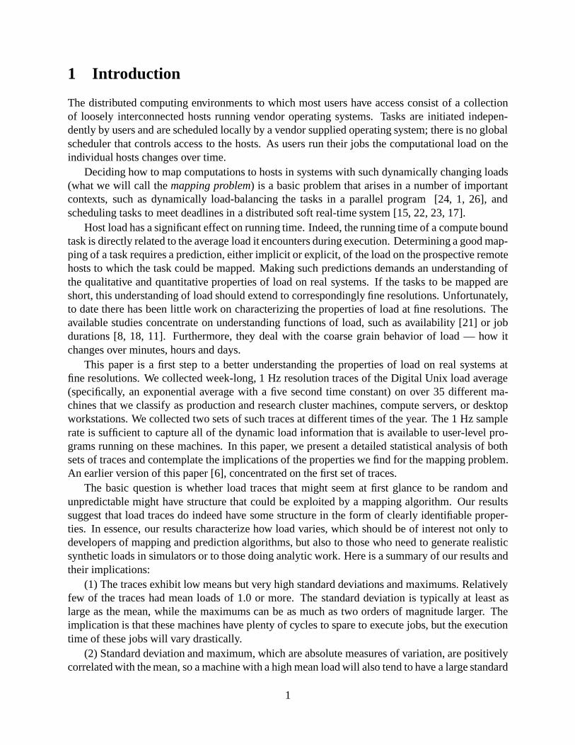
Figures 1 and 2 provide additional details of the individual August, 1997 and March, 1998traces. The author will be happy to provide the traces to any interested readers.

3 Statistical analysis

We analyzed the individual load traces using summary statistics, histograms, fitting of analyticdistributions, and time series analysis. The picture that emerges is that load varies over a widerange in very complex ways. Load distributions are rough and frequently multi-modal. Even

3

Hostname Start Time Days SamplesProduction Cluster

axp0.psc Tue Aug 12 21:29:12 EDT 1997 15.00 1296000axp1.psc Tue Aug 12 21:30:09 EDT 1997 14.00 1209600axp2.psc Tue Aug 12 21:30:53 EDT 1997 14.00 1209600axp3.psc Tue Aug 12 21:31:13 EDT 1997 14.00 1209600axp4.psc Tue Aug 12 21:31:12 EDT 1997 14.00 1209600axp5.psc Tue Aug 12 21:31:47 EDT 1997 14.00 1209600axp6.psc Tue Aug 12 21:31:15 EDT 1997 15.00 1296000axp7.psc Tue Aug 12 20:51:19 EDT 1997 13.00 1123200axp8.psc Tue Aug 12 21:31:19 EDT 1997 14.00 1209600axp9.psc Tue Aug 12 21:31:45 EDT 1997 14.00 1209600axp10.psc Tue Aug 12 21:31:21 EDT 1997 14.00 1209600axpfea.psc Sat Aug 16 14:44:29 EDT 1997 13.00 1123200axpfeb.psc Sat Aug 16 14:44:55 EDT 1997 12.00 1036800

Research Clustermanchester-1.cmcl Sun Aug 17 19:41:10 EDT 1997 3.92 338400manchester-2.cmcl Sun Aug 17 19:41:09 EDT 1997 4.00 345600manchester-3.cmcl Sun Aug 17 19:41:13 EDT 1997 3.96 342000manchester-4.cmcl Sun Aug 17 19:41:10 EDT 1997 4.00 345600manchester-5.cmcl Sun Aug 17 19:41:09 EDT 1997 4.04 349200manchester-6.cmcl Sun Aug 17 19:41:09 EDT 1997 4.08 352800manchester-7.cmcl Sun Aug 17 19:41:10 EDT 1997 4.00 345600manchester-8.cmcl Sun Aug 17 19:41:10 EDT 1997 4.00 345600

Compute Serversmojave.cmcl Sun Aug 17 19:41:11 EDT 1997 4.04 349200sahara.cmcl Sun Aug 17 19:41:11 EDT 1997 4.00 345600

Desktopsaphrodite.nectar Sun Aug 17 19:41:12 EDT 1997 4.00 345600argus.nectar Sun Aug 17 19:41:17 EDT 1997 4.04 349200asbury-park.nectar Sun Aug 17 19:41:11 EDT 1997 4.00 345600asclepius.nectar Sun Aug 17 19:41:07 EDT 1997 4.08 352800bruce.nectar Sun Aug 17 19:41:10 EDT 1997 3.92 338400cobain.nectar Sun Aug 17 19:41:12 EDT 1997 4.04 349200darryl.nectar Sun Aug 17 19:41:32 EDT 1997 1.71 147600hawaii.cmcl Sun Aug 17 19:41:11 EDT 1997 2.63 226800hestia.nectar Sun Aug 17 19:41:12 EDT 1997 4.00 345600newark.cmcl Sun Aug 17 19:41:13 EDT 1997 4.00 345600pryor.nectar Sun Aug 17 19:41:13 EDT 1997 1.71 147600rhea.nectar Sun Aug 17 19:41:11 EDT 1997 4.00 345600rubix.mc Sun Aug 17 19:41:13 EDT 1997 4.00 345600themis.nectar Sun Aug 17 19:41:09 EDT 1997 4.00 345600uranus.nectar Sun Aug 17 19:41:13 EDT 1997 4.00 345600zeno.nectar Sun Aug 17 19:41:13 EDT 1997 4.08 352800

Figure 1: Details of the August, 1997 traces.

4

Hostname Start Time Days SamplesProduction Cluster

axp0.psc Wed Feb 25 17:34:26 EST 1998 12.08 1043400axp1.psc Wed Feb 25 17:34:25 EST 1998 12.08 1043400axp2.psc Wed Feb 25 17:34:25 EST 1998 12.08 1043400axp3.psc Wed Feb 25 17:34:26 EST 1998 12.03 1039400axp4.psc Wed Feb 25 17:34:27 EST 1998 12.06 1041900axp5.psc Wed Feb 25 17:34:27 EST 1998 12.03 1039700axp6.psc Wed Feb 25 17:34:27 EST 1998 12.08 1043400axp7.psc Wed Feb 25 17:34:27 EST 1998 12.01 1037700axp8.psc Wed Feb 25 17:34:28 EST 1998 12.06 1041800axp10.psc Wed Feb 25 17:34:28 EST 1998 12.03 1039700axp11.psc Wed Feb 25 17:16:20 EST 1998 12.03 1039800axpfea.psc Wed Feb 25 17:18:01 EST 1998 12.08 1043800axpfeb.psc Wed Feb 25 17:23:34 EST 1998 12.0 1043400

Research Clustermanchester-1.cmcl Wed Feb 25 20:42:30 EST 1998 8.36 721900manchester-2.cmcl Wed Feb 25 20:42:23 EST 1998 8.36 721900manchester-3.cmcl Wed Feb 25 20:42:23 EST 1998 8.36 721900manchester-4.cmcl Wed Feb 25 20:42:29 EST 1998 8.35 721300manchester-5.cmcl Wed Feb 25 20:42:27 EST 1998 8.36 721900manchester-6.cmcl Wed Feb 25 20:42:30 EST 1998 8.36 721900manchester-7.cmcl Wed Feb 25 20:42:24 EST 1998 8.35 721800manchester-8.cmcl Wed Feb 25 20:42:26 EST 1998 8.35 721800

Compute Serversmojave.cmcl Wed Feb 25 20:42:31 EST 1998 5.31 458800sahara.cmcl Wed Feb 25 20:42:34 EST 1998 8.34 721300

Desktopsaphrodite Wed Feb 25 20:42:17 EST 1998 8.36 722000asbury-park Wed Feb 25 20:42:23 EST 1998 5.90 509400belushi Wed Feb 25 20:42:28 EST 1998 7.77 671400hawaii Wed Feb 25 20:42:18 EST 1998 8.36 722000loman Wed Feb 25 20:42:34 EST 1998 8.36 721900newark.cmcl Wed Feb 25 20:42:29 EST 1998 8.36 722200pryor.nectar Wed Feb 25 20:42:24 EST 1998 8.36 722100rhea.nectar Wed Feb 25 21:12:17 EST 1998 10.19 880600rubix.mc Wed Feb 25 20:42:24 EST 1998 1.81 156400themis.nectar Wed Feb 25 20:42:29 EST 1998 4.94 426900uranus.nectar Wed Feb 25 20:42:33 EST 1998 8.36 722000zeno.nectar Wed Feb 25 20:42:26 EST 1998 6.23 537900

Figure 2: Details of the March, 1998 traces.

5

MeanLoad

SdevLoad

COVLoad

MaxLoad

Max/MeanLoad

MeanEpoch

SdevEpoch

COVEpoch

HurstParam

Entropy

Mean Load 1.00Sdev Load 0.53 1.00COV Load -0.49 -0.22 1.00Max Load 0.60 0.18 -0.32 1.00Max/Mean Load -0.36 -0.39 0.51 0.03 1.00Mean Epoch -0.04 -0.10 -0.19 0.08 -0.05 1.00Sdev Epoch -0.02 -0.10 -0.20 0.09 -0.06 0.99 1.00COV Epoch 0.07 -0.11 -0.23 0.15 -0.02 0.95 0.96 1.00Hurst Param 0.45 0.58 -0.21 0.03 -0.49 0.08 0.10 0.18 1.00Entropy 0.42 0.51 -0.10 0.40 -0.36 -0.27 -0.25 -0.30 0.24 1.00

(a) Correlations for August, 1997 tracesMeanLoad

SdevLoad

COVLoad

MaxLoad

Max/MeanLoad

MeanEpoch

SdevEpoch

COVEpoch

HurstParam

Entropy

Mean Load 1.00Sdev Load 0.72 1.00COV Load -0.64 -0.48 1.00Max Load 0.43 0.11 -0.25 1.00Max/Mean Load -0.48 -0.49 0.93 -0.07 1.00Mean Epoch -0.12 -0.23 -0.08 0.17 -0.05 1.00Sdev Epoch -0.13 -0.22 -0.09 0.15 -0.06 0.99 1.00COV Epoch -0.03 -0.12 -0.15 0.23 -0.11 0.88 0.93 1.00Hurst Param -0.30 -0.41 0.29 0.15 0.36 0.92 0.90 0.78 1.00Entropy 0.05 0.27 -0.19 -0.05 -0.27 -0.19 -0.18 -0.17 -0.29 1.00

(b) Correlations for March, 1998 traces

Figure 3: Correlation coefficients (CCs) between all of the discussed statistical properties.

traces with unimodal histograms are not well fitted by common analytic distributions, which havetails that are either too short or too long. Time series analysis shows that load is strongly correlatedover time, but also has complex, almost noise-like frequency domain behavior.

We summarized each of our load traces in terms of our statistical measures and computed theircorrelations to determine how the measures are related. Figure 3(a) contains the correlations forthe August, 1997 set while Figure 3(b) contains the correlations for the March, 1998 set. Unlessotherwise noted, the remaining figures in the paper similarly present independent results for thetwo sets of traces. Each cell of the tables in Figure 3 is the correlation coefficient (CC) between therow measure and the column measure, computed over the the load traces in the set. We will referback to the highlighted cells (where the absolute correlations are greater than 0.3) throughout thepaper. It is important to note that these cross correlations can serve as a basis for clustering loadtraces into rough equivalence classes.

Summary statistics:

Summarizing each load trace in terms of its mean, standard deviation, and maximum and minimumillustrates the extent to which load varies. Figure 4 shows the mean load and the +/- one standarddeviation points for each of the traces. As we might expect, the mean load on desktop machines issignificantly lower than on other machines. However, we can also see a lack of uniformity withineach class, despite the long duration of the traces. This is most clear among the Production Clustermachines, where fewer than half of the machines seem to be doing most of the work. This lackof uniformity even over long time scales shows clear opportunity for load balancing or resourcemanagement systems.

From Figure 4 we can also see that desktop machines have smaller standard deviations than the

6

-0.4

-0.2

0

0.2

0.4

0.6

0.8

1

1.2

1.4

1.6

1.8

Host

+SDev

-SDev

Mean

Production Cluster ResearchCluster

Desktops

-0.4

-0.2

0

0.2

0.4

0.6

0.8

1

1.2

1.4

1.6

1.8

Host

+SDev

-SDev

Mean

Production Cluster ResearchCluster

Desktops

(a) (b)

Figure 4: Mean load +/- one standard deviation: (a) August, 1997 traces, (b) March, 1998 traces.

0

2

4

6

8

10

12

0

0.2

0.4

0.6

0.8

1

1.2

1.4

Host

Production Cluster ResearchCluster

Desktops

0

2

4

6

8

10

12

0

0.2

0.4

0.6

0.8

1

1.2

1.4

Host

Production Cluster ResearchCluster

Desktops

(a) (b)

Figure 5: COV of load and mean load: (a) August, 1997 traces, (b) March, 1998 traces.

7

0

2

4

6

8

10

12

Host

Max

Min

Mean

Production Cluster ResearchCluster

Desktops

0

2

4

6

8

10

12

Host

Max

Min

Mean

Production Cluster ResearchCluster

Desktops

(a) (b)

Figure 6: Minimum, maximum, and mean load: (a) August, 1997 traces, (b) March, 1998 traces.

other machines. Indeed, the standard deviation, which shows how much load varies inabsoluteterms, grows with increasing mean load (Figure 3 shows CC=0.53 for the 1997 traces and CC=0.72for the 1998 traces.) However, inrelative terms, variance shrinks with increasing mean load. Thiscan be seen in Figure 5, which plots the coefficient of variation (the standard deviation divided bythe mean, abbreviated as the COV) and the mean load for each of the load traces. Here we cansee that desktop machines, with their smaller mean loads, have large COVs compared to the otherclasses of machines. The CC between mean load and the COV of load is -0.49 for the 1997 tracesand -0.64 for the 1998 traces. It is clear that as load increases, it varieslessin relative terms andmorein absolute terms.

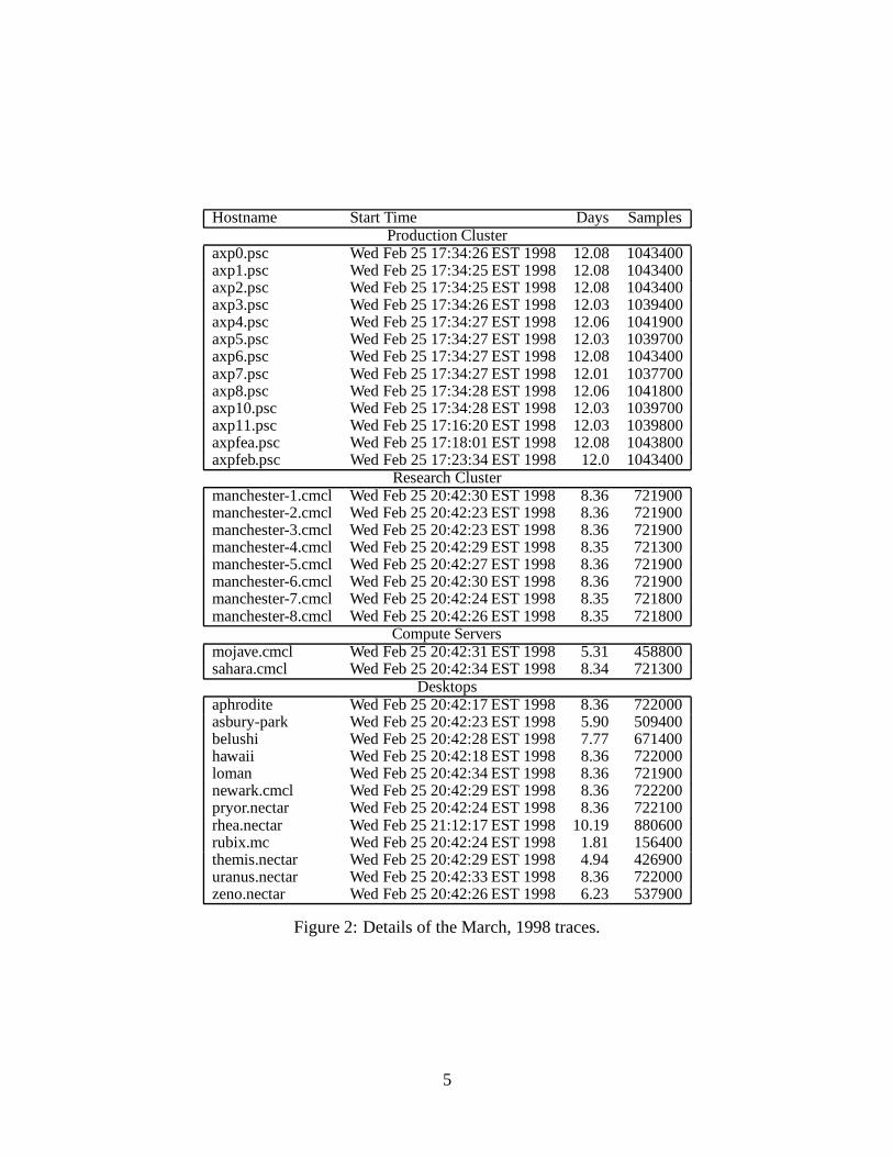
This difference between absolute and relative behavior also holds true for the maximum load.Figure 6 shows the minimum, maximum, and mean load for each of the traces. The minimumload is, not surprisingly, zero in almost every case. The maximum load is positively correlatedwith the mean load (CC=0.60 for the 1997 traces and CC=0.43 for the 1998 traces in Figure 3.)Figure 7 plots the ratio max/mean and the mean load for each of the traces. It is clear that thisrelative measure is inversely related to mean load, and Figure 3 shows that the CC is -0.36 for the1997 traces and -0.48 for the 1998 traces. It is also important to notice that while the differencesin maximum load between the hosts are rather small (Figure 6), the differences in the max/meanratio can be quite large (Figure 7.) Desktops are more surprising machines in relative terms.

With respect to the mapping problem, the implication of the differences between relative andabsolute measures of variability is that lightly loaded (low mean load) hosts are not always prefer-able over heavily loaded hosts. For example, if the performance metric is itself a relative one (thatthe execution time not vary much relative to the mean execution time, say), then a more heavilyloaded host may be preferable.

Distributions:

We next treated each trace as a realization of an independent, identically distributed(IID) stochasticprocess. Such a process is completely described by its probability distribution function (pdf),which does not change over time. Since we have a vast number of data points for each trace,

8

0

50

100

150

200

250

300

350

400

0

0.2

0.4

0.6

0.8

1

1.2

1.4

Host

Production Cluster ResearchCluster

Desktops

0

50

100

150

200

250

300

350

400

0

0.2

0.4

0.6

0.8

1

1.2

1.4

Host

Production Cluster ResearchCluster

Desktops

(a) (b)

Figure 7: Maximum to mean load ratios and mean load: (a) August, 1997 traces, (b) March, 1998traces.

0 1 2 3 40

0.5

1

1.5

2

2.5

3x 10

4

Load

Num

ber

of o

bser

vatio

ns

0 0.5 1 1.50

0.5

1

1.5

2

2.5

3

3.5x 10

4

Load

Num

ber

of o

ccur

ance

s

(a) axp0 (b) axp7

Figure 8: Histograms for load on axp0 and axp7 on August 19, 1997.

9

−0.4 −0.2 0 0.2 0.4 0.6−0.5

0

0.5

1

1.5

Quantiles of fitted Normal

Qua

ntile

s of

axp

7

0 0.5 1 1.5−0.5

0

0.5

1

1.5

2

2.5

Quantiles of fitted Exponential

Qua

ntile

s of

axp

7

(a) axp7 versus normal (b) axp7 versus exponential

Figure 9: Quantile-quantile plots for axp7 trace of August 19, 1997.

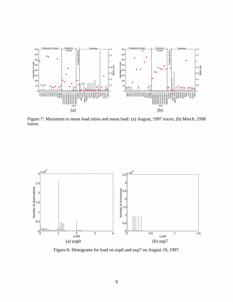
histograms closely approximate this underlying pdf. We examined the histograms of each of ourload traces and fitted normal and exponential distributions to them. To illustrate the followingdiscussion, Figure 8 shows the histograms of load measurements on (a) axp0 and (b) axp7 onAugust 19, 1997 (86400 samples each.) Axp0 has a high mean load, while axp7 is much morelightly loaded.

Some of the traces, especially those with high mean loads, have multi-modal histograms. Fig-ure 8(a) is an example of such a multi-modal distribution while Figure 8(b) shows a unimodaldistribution. Typically, the modes are integer multiples of 1.0 (and occasionally 0.5.) One explana-tion for this behavior is that jobs on these machines are for the most part compute bound and thusthe ready queue length corresponds to the number of jobs. This seems plausible for the cluster ma-chines, which run scientific workloads for the most part. However, such multi-modal distributionswere also noticed on the some of the other machines.

The rough appearance of the histograms (consider Figure 8(b)) is due to the fact that the under-lying quantity being measured (ready queue length) is discrete. Load typically takes on 600-3000unique values in these traces. Shannon’s entropy measure [25] indicates that the load traces can beencoded in 1.4 to 8.5 bits per value, depending on the trace. These observations and the histogramssuggest that load spends most of its time in one of a small number of levels.

The histograms share very few common characteristics and did not conform well to the analyticdistributions we fit to them. Quantile-quantile plots are a powerful way to assess how a distributionfits data (cf. [14], pp. 196–200.) The quantiles (the� quantile of a pdf (or histogram) is the valuexat which100� % of the probability (or data) falls to the left ofx) of the data set are plotted againstthe quantiles of the hypothetical analytic distribution. Regardless of the choice of parameters, theplot will be linear if the data fits the distribution.

We fitted normal and exponential distributions to each of the load traces. The fits are atrociousfor the multimodal traces, and we do not discuss them here. For the unimodal traces, the fits areslightly better. Figure 9 shows quantile-quantile plots for (a) normal and (b) exponential distri-butions fitted to the unimodal axp7 load trace of Figure 8(b). Neither the normal or exponentialdistribution correctly captures the tails of the load traces. This can be seen in the figure. The

10

0 6 12 18 240

0.5

1

1.5

Time (hours)

Load

0 100 200 300 400 500 6000

0.2

0.4

0.6

0.8

1

Lag (seconds)

AC

F

(a) (b)

0 0.510

−2

100

102

104

Frequency (Hz)

Mag

nitu

de

0 100 200 300 400 500 600−1

−0.5

0

0.5

1

Lag (seconds)

PA

CF

(d) (c)

Figure 10: Time series analysis of axp7 load trace collected on August 19, 1997: (a) Load trace,(b) Autocorrelation function to lag 600 (10 minutes), (c) Partial autocorrelation function to lag 600(10 minutes), (d) Periodogram.

quantiles of the data grow faster than those of the normal distribution toward the right sides ofFigure 9(a). This indicates that the data has a longer or heavier tail than the normal distribution.Conversely, the quantiles of the data grow more slowly than those of the exponential distribution,as can be seen in Figures 9(b). This indicates that the data has a shorter tail than the exponentialdistribution. Notice that the exponential distribution goes ase�x while the normal distribution goesase�x

2

.

There are two implications of these complex distributions. First, simulation studies and analyticresults predicated on simple, analytic distributions may produce erroneous results. Clearly, trace-driven simulation studies are to be preferred. The second implication is that prediction algorithmsshould not only reduce the overall variance of the load signal, but also produce errors that are betterfit an analytic distribution. One reason for this is to make confidence intervals easier to compute.

11

Time series analysis:

We examined the autocorrelation function, partial autocorrelation function, and periodogram ofeach of the load traces. These time series analysis tools show that past load values have a stronginfluence on future load values. For illustration, Figure 10 shows (a) the axp7 load trace collectedon August 19, 1997, (b) its autocorrelation function to a lag of 600, (c) its partial autocorrelationfunction to a lag of 600, and (d) its periodogram. The analysis of this trace is representative of ourresults.

The autocorrelation function, which ranges from -1 to 1, shows how well a load value at timet is linearly correlated with its corresponding load value at timet + � — in effect, how well thevalue at timet linearly predicts the value at timet+�. Autocorrelation is a function of�, and inFigure 10(b) we show the results for0 � � � 600. Notice that even at� = 600 seconds, valuesare still strongly correlated. This very strong, long range correlation is common to each of the loadtraces.

The partial autocorrelation function shows how well purely autoregressive linear models cap-ture the correlation structure of a sequence [4], pp. 64–69. The square of the value of the functionat a lagk indicates the benefit of advancing from ak � 1-th order model to ak-th order model.Intuitively, if a k-th order model were sufficient, then the partial autocorrelation function would bezero beyond a lag ofk and the autocorrelation function would be infinite. In a dual manner, if ak-th order purely moving average model were sufficient, then the autocorrelation function wouldbe zero beyond a lag ofk and the partial autocorrelation function would be infinite. As we cansee from Figure 10(b) and (c), both functions have extremely large extents. This suggests thatmixed models, which combine autoregressive and moving average components are appropriate formodelling host load.

The periodogram of a load trace is the magnitude of the Fourier transform of the load data,which we plot on a log scale (Figure 10(d).) The periodogram shows the contribution of differentfrequencies (horizontal axis) to the signal. What is clear in the figure, and is true of all of the loadtraces, is that there are significant contributions from all frequencies — the signal looks much likenoise. We believe the two noticeable peaks to be artifacts of the kernel sample rate — the kernelis not sampling the length of the ready queue frequently enough to avoid aliasing. Only a few ofthe other traces exhibit the smaller peaks, but they all share the broad noise-like appearance of thistrace.

There are several implications of this time series analysis. First, the existence of such strongautocorrelation implies that load prediction based on past load values is feasible. It also suggeststhat simulation models and analytical work that eschews this very clear dependence may be inerror. Finally, the almost noise-like periodograms suggest that quite complex, possibly nonlinearmodels will be necessary to produce or predict load.

4 Self-similarity

The key observation of this section is that each of the load traces exhibits a high degree of self-similarity. This is significant for two reasons. First, it means that load varies significantly acrossall time-scales — it is not the case that increasing smoothing of the load quickly tames its variance.A job will have a great deal of variance in its running time regardless of how long it is. Second, it

12

0 2 4 6 8 10 12

x 105

0

0.2

0.4

0.6

0.8

1

1.2

1.4

1.6

1.8axp7 − 1 to 1123200 (1123200 seconds)

time (seconds)

load

5.59 5.595 5.6 5.605 5.61 5.615 5.62 5.625 5.63 5.635 5.64

x 105

0

0.1

0.2

0.3

0.4

0.5

0.6

0.7axp7 − 559407 to 563793 (4387 seconds)

time (seconds)

load

10 days 64 minutes

4 4.5 5 5.5 6 6.5 7 7.5

x 105

0

0.5

1

1.5axp7 − 421200 to 702000 (280801 seconds)

time (seconds)

load

5.61 5.612 5.614 5.616 5.618 5.62 5.622

x 105

0

0.1

0.2

0.3

0.4

0.5

0.6

0.7axp7 − 561052 to 562148 (1097 seconds)

time (seconds)

load

2.5 days 16 minutes

5.2 5.3 5.4 5.5 5.6 5.7 5.8 5.9 6

x 105

0

0.5

1

1.5axp7 − 526500 to 596700 (70201 seconds)

time (seconds)

load

5.6145 5.615 5.6155 5.616 5.6165 5.617 5.6175

x 105

0.12

0.14

0.16

0.18

0.2

0.22

0.24

0.26

0.28

0.3axp7 − 561463 to 561737 (275 seconds)

time (seconds)

load

16 hours 4 minutes

5.52 5.54 5.56 5.58 5.6 5.62 5.64 5.66 5.68 5.7 5.72

x 105

0

0.1

0.2

0.3

0.4

0.5

0.6

0.7

0.8

0.9axp7 − 552825 to 570375 (17551 seconds)

time (seconds)

load

5.6156 5.6157 5.6158 5.6159 5.616 5.6161 5.6162 5.6163 5.6164

x 105

0.12

0.14

0.16

0.18

0.2

0.22

0.24

0.26

0.28

0.3axp7 − 561566 to 561634 (69 seconds)

time (seconds)

load

4 hours 60 seconds

Figure 11: Visual representation of self-similarity. Each graph plots load versus time and “zoomsin” on the middle quarter

13

0.01

0.1

1

10

100

1000

10000

100000

0.0001 0.001 0.01 0.1 1Log(Frequency)

H=0.375

H=0.5

H=0.625H=0.875

H=(1-slope)/2

0.1

1

2

1 10 100 1000 10000Bin Size

H=0.5H=0.625

H=0.375

H=0.95

H=1+slope

(a) (b)

Figure 12: Meaning of the Hurst parameter: (a) Frequency domain interpretation using powerspectral analysis, (b) Effect of increased smoothing using dispersional analysis.

suggests that load is difficult to model and predict well. In particular, self-similarity is indicative oflong memory, possibly non-stationary stochastic processes such as fractional ARIMA models [12,10, 3], and fitting such models to data and evaluating them can be quite expensive.

Figure 11 visually demonstrates the self similarity of the axp7 load trace. The top left graph inthe figure plots the load on this machine versus time for 10 days. Each subsequent graph “zoomsin” on the highlighted central 25% of the previous graph, until we reach the bottom right graph,which shows the central 60 seconds of the trace. The plots are scaled to make the behavior on eachtime scale obvious. In particular, over longer time scales, wider scales are necessary. Intuitively, aself-similar signal is one that looks similar on different time scales given this rescaling. Althoughthe behavior on the different graphs is not identical, we can clearly see that there is significantvariation on all time scales.

An important point is that as we smooth the signal (as we do visually as we “zoom out” towardthe top of the page in Figure 11), the load signal strongly resists becoming uniform. This suggeststhat low frequency components are significant in the overall mix of the signal, or, equivalently,that there is significant long range dependence. It is this property of self-similar signals that moststrongly differentiates them and causes significant modeling difficulty.

Self-similarity is more than intuition — it is a well defined mathematical statement about therelationship of the autocorrelation functions of increasingly smoothed versions of certain kinds oflong-memory stochastic processes. These stochastic processes model the sort of the mechanismsthat give rise to self-similar signals. We shall avoid a mathematical treatment here, but interestedreaders may want to consult [19] or [20] for a treatment in the context of networking or [2] forits connection to fractal geometry, or [3] for a treatment from a linear time series point of view.Interestingly, self-similarity has revolutionized network traffic modelling in the 1990s [9, 19, 20,28].

The degree and nature of the self-similarity of a sequence is summarized by the Hurst param-eter,H [13]. Intuitively, H describes the relative contribution of low and high frequency com-ponents to the signal. Consider Figure 12(a), which plots the periodogram (the magnitude of the

14

0

0.2

0.4

0.6

0.8

1

1.2

Host

Production Cluster ResearchCluster

Desktops

+SDev

-SDev

Mean

0

0.2

0.4

0.6

0.8

1

1.2

Host

Production Cluster ResearchCluster

Desktops

+SDev

-SDev

Mean

(a) (b)

Figure 13: Hurst parameter estimates (mean of four point estimates and standard deviation) : (a)August, 1997 traces, (b) March, 1998 traces.

Fourier transform) of the axp7 load trace of August 19, 1997 on a log-log scale. In this transformedform, we can describe the trend with a line of slope�� (meaning that the periodogram decays hy-perbolically with frequency! as!��. The Hurst parameterH is then defined asH = (1 + �)=2.As we can see in Figure 12(a),H = 0:5 corresponds to a line of zero slope. This is the uncorrelatednoise case, where all frequencies make a roughly equal contribution. AsH increases beyond0:5,we see that low frequencies make more of a contribution. Similarly, asH decreases below0:5,low frequencies make less of a contribution.H > 0:5 indicates self-similarity with positive nearneighbor correlation, whileH < 0:5 indicates self-similarity with negative near neighbor correla-tion. Figure 12(a) shows that the axp7 trace is indeed self-similar withH = 0:875. This methodof determining the Hurst parameter is known as power spectral analysis.

Figure 12(b) illustrates another way to think about the Hurst parameterH. To create the figure,we binned the load trace with increasingly larger, non-overlapping bins and then plotted the relativedispersion (the standard deviation normalized by the mean) of the binned series versus the size ofthe bins. For example, at a bin size of 8 we averaged the first 8 samples of the original series toform the first sample of the binned series, the next 8 to form the second sample, and so on. Thefigure shows that the relative dispersion of this new 8-binned series is slightly less than one. Ifthe original load trace is self-similar, the relative dispersion should decline hyperbolically withincreasing bin size. On a log-log scale such we use in the figure this relationship would appear tobe linear with a slope ofH � 1. We see that this is indeed the case for the axp7 trace. Notice thatthis method for estimatingH, which is called dispersional analysis, gives a slightly differentH

(0.95) than power spectral analysis. What is important is that in both figures we see a hyperbolicrelationship, and that both estimates forH are much larger than 0.5.

We examined each of the load traces for self-similarity and estimated each one’s Hurst param-eter. There are many different estimators for the Hurst parameter [27], but there is no consensuson how to best estimate the Hurst parameter of a measured series. The most common technique isto use several Hurst parameter estimators and try to find agreement among them. The four Hurstparameter estimators we used were R/S analysis, the variance-time method, dispersional analy-

15

0

0.2

0.4

0.6

0.8

1

1.2

Host

R/S Analysis

Variance-Time Method

Dispersional Analysis

Power Spectral Analysis

Production Cluster ResearchCluster

Desktops

0

0.2

0.4

0.6

0.8

1

1.2

Host

R/S Analysis

Variance-Time

Dispersional Analysis

Power Spectral Analysis

Production Cluster ResearchCluster

Desktops

(a) (b)

Figure 14: Hurst parameter point estimates: (a) August, 1997 traces, (b) March, 1998 traces.

sis, and power spectral analysis. A description of these estimators as well as several others may befound in [2]. The advantage of these estimators is that they make no assumptions about the stochas-tic process that generated the sequence. However, they also cannot provide confidence intervalsfor their estimates. Estimators such as the Whittle estimator [3] can provide confidence intervals,but a stochastic process model must be assumed over which anH can be found that maximizes itslikelihood.

We implemented the estimators using Matlab and validated each one by examining degenerateseries with knownH and series with specificH generated using the random midpoint displacementmethod. The dispersional analysis method was found to be rather weak forH values less than about0:8 and the power spectral analysis method gave the most consistent results.

Figure 13 presents our estimates of the Hurst parameters of each of load traces. In the graph,each central point is the mean of the four estimates, while the outlying points are at +/- one standarddeviation. Figure 14 shows the four actual point estimates for each trace. Notice that for smallH

values, the standard deviation is high due to the inaccuracy of dispersional analysis. The importantpoint is that the mean Hurst estimates are all significantly above theH = 0:5 line and their +/- onestandard deviation points are also above the line.

The traces exhibit self-similarity Hurst parameters ranging from 0.73 to 0.99, with a strongbias toward the top of that range. An examination of the correlation coefficients (CCs) in Figure 3shows some surprising results. For the August, 1997 traces, the Hurst parameter is positively cor-related with mean load (CC=0.45) and the standard deviation of load (CC=0.58), but is negativelycorrelated with the max/mean load ratio (CC=-0.49). On the other hand, for the March, 1998traces, the Hurst parameter is negatively correlated with mean load (CC=-0.30) and the standarddeviation of load (CC=-0.41), but is positively correlated with the max/mean ratio (CC=0.36). Fur-thermore, in the March, 1998 traces, we find the Hurst parameter is strongly positively correlatedwith the epoch statistics, which is not the case at all for the August, 1997 traces. It is not clearwhat the cause for this difference between the traces is.

As we discussed above, self-similarity has implications for load modeling and for load smooth-ing. The long memory stochastic process models that can capture self-similarity tend to be expen-

16

sive to fit to data and evaluate. Smoothing the load (by mapping large units of computations insteadof small units, for example) may be misguided since variance may not decline with increasingsmoothing intervals as quickly as quickly as expected. Consider smoothing load by averaging overan interval of lengthm. Without long range dependence (H = 0:5), variance would decay withm asm�1:0, while with long range dependence, asm2H�2 or m�0:54 andm�0:02 for the range ofHurst parameters we measured.

5 Epochal behavior

The key observation in this section is that while load changes in complex ways, the manner inwhich it changes remains relatively constant for relatively long periods of time. We refer to aperiod of time in which this stability holds true as an epoch. For example, the load signal could bea 0.25 Hz Sin wave for a minute and a 0.125 Hz sawtooth wave the next minute — each minuteis an epoch. That these epochs exist and are long is significant because it suggests that modelingload can be simplified by modeling epochs separately from modeling the behavior within an epoch.Similarly, it suggests a two stage prediction process.

The spectrogram representation of a load trace immediately highlights the epochal behavior wediscuss in this section. A spectrogram combines the frequency domain and time domain represen-tations of a time series. It shows how the frequency domain changes locally (for a small segmentof the signal) over time. For our purposes, this local frequency domain information is the “mannerin which [the load] changes” to which we referred earlier. To form a spectrogram, we slide a win-dow of lengthw over the series, and at each offsetk, we Fourier-transform thew elements in thewindow to give usw complex Fourier coefficients. Since our load series is real-valued, only thefirst w=2 of these coefficients are needed. We form a plot where thex coordinate is the offsetk,they coordinate is the coefficient number,1; 2; : : : ; w=2 and thez coordinate is the magnitude ofthe coefficient. To simplify presentation, we collapse to two dimensions by mapping the logarithmof thez coordinate (the magnitude of the coefficient) to color. The spectrogram is basically a mid-point in the tradeoff between purely time-domain or frequency-domain representations. Along thex axis we see the effects of time and along they axis we see the effects of frequency.

Figure 15 shows a representative case, a 24 hour trace from the PSC host axp7, taken on August19, 1997. The top graph shows the time domain representation, while the bottom graph shows thecorresponding spectrogram representation. What is important to note (and which occurs in allthe spectrograms of all the traces) are the relatively wide vertical bands. These indicate that thefrequency domain of the underlying signal stays relatively stable for long periods of time. We referto the width of a band as the duration of that frequency epoch.

That these epochs exist can be explained by programs executing different phases, programsbeing started and shut down, and the like. The frequency content within an epoch contains energyat higher frequencies because of events that happen on smaller time-frames, such as user input,device driver execution, and daemon execution.

We can algorithmically find the edges of these epochs by computing the difference in adja-cent spectra in the spectrogram and then looking for those offsets where the differences exceeda threshold. Specifically, we compute the sum of mean squared errors for each pair of adjacentspectra. The elements of this error vector are compared to an epsilon (5% here) times the mean ofthe vector. Where this threshold is exceeded, a new epoch is considered to begin. Having found

17

0 6 12 18 240

0.5

1

1.5

Time (hours)

Load

Time (hours)

Fre

quen

cy (

Hz)

0 6 12 18 240

0.1

0.2

0.3

0.4

0.5

Figure 15: Time domain and spectrogram representations of load for host axp7 on August 19,1997.

18

-200

0

200

400

600

800

1000

1200

Host

+SDev

-SDev

Mean

Production Cluster ResearchCluster

Desktops

-200

0

200

400

600

800

1000

1200

Host

+SDev

-SDev

Mean

Production Cluster ResearchCluster

Desktops

(a) (b)

Figure 16: Mean epoch length +/- one standard deviation: (a) August, 1997 traces, (b) March,1998 traces.

the epochs, we can examine their statistics. Figure 16 shows the mean epoch length and the +/- onestandard deviation levels for each of the load traces. The mean epoch length ranges from about 150seconds to over 450 seconds, depending on which trace. The standard deviations are also relativelyhigh (80 seconds to over 600 seconds.) It is the Production Cluster class which is clearly differentwhen it comes to epoch length. The machines in this class tend to have much higher means andstandard deviations than the other machines. One explanation might be that most of the machinesrun batch-scheduled scientific jobs which may well have longer computation phases and runningtimes. However, two of the interactive machines also exhibit high means and standard deviations.Interestingly, there is no correlation of the mean epoch length and standard deviation to the meanload for either set of traces (Figure 3.) However, for the March, 1998 traces, we find correlationsbetween the epoch length statistics and the Hurst parameter that are particularly strong. It is notclear why this difference exists between the traces.

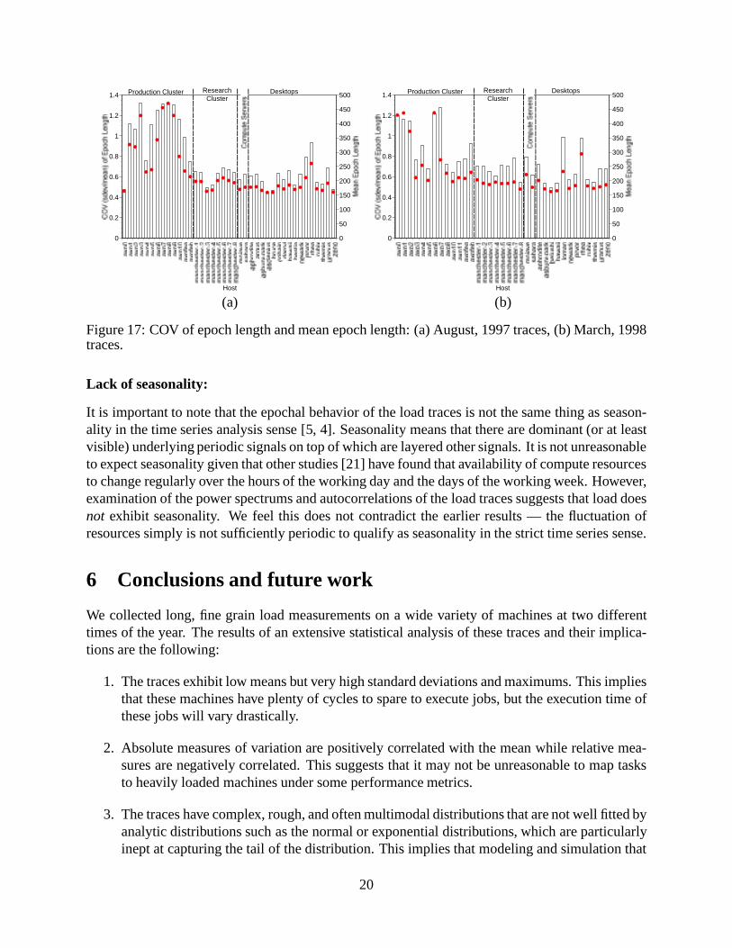
The standard deviations of epoch length in Figure 16 give us an absolute measure of the vari-ance of epoch length. Figure 17 shows the coefficient of variance (COV) of epoch length and meanepoch length for each trace. The COV is our relative measure of epoch length variance. Unlikewith load (Section 3), these absolute and relative measures of epoch length variance arebothposi-tively correlated with the mean epoch length. In addition, the correlation is especially strong (theCCs are at least 0.88.) As epoch length increases, it varies more in both absolute and relative terms.The statistical properties of epoch lengths are independent of the statistical properties of load.

The implication of long epoch lengths is that the problem of predicting load may be able to bedecomposed into a segmentation problem (finding the epochs) and a sequence of smaller predictionsubproblems (predicting load within each epoch.)

Strictly speaking, epochal behavior means that load is not stationary. However, it is also notfree to wander at will — clearly load cannot rise to infinite levels or fall below zero. This iscompatible with the “borderline stationarity” implied by self-similarity.

19

0

0.2

0.4

0.6

0.8

1

1.2

1.4

0

50

100

150

200

250

300

350

400

450

500

Host

Production Cluster ResearchCluster

Desktops

0

0.2

0.4

0.6

0.8

1

1.2

1.4

0

50

100

150

200

250

300

350

400

450

500

Host

Production Cluster ResearchCluster

Desktops

(a) (b)

Figure 17: COV of epoch length and mean epoch length: (a) August, 1997 traces, (b) March, 1998traces.

Lack of seasonality:

It is important to note that the epochal behavior of the load traces is not the same thing as season-ality in the time series analysis sense [5, 4]. Seasonality means that there are dominant (or at leastvisible) underlying periodic signals on top of which are layered other signals. It is not unreasonableto expect seasonality given that other studies [21] have found that availability of compute resourcesto change regularly over the hours of the working day and the days of the working week. However,examination of the power spectrums and autocorrelations of the load traces suggests that load doesnot exhibit seasonality. We feel this does not contradict the earlier results — the fluctuation ofresources simply is not sufficiently periodic to qualify as seasonality in the strict time series sense.

6 Conclusions and future work

We collected long, fine grain load measurements on a wide variety of machines at two differenttimes of the year. The results of an extensive statistical analysis of these traces and their implica-tions are the following:

1. The traces exhibit low means but very high standard deviations and maximums. This impliesthat these machines have plenty of cycles to spare to execute jobs, but the execution time ofthese jobs will vary drastically.

2. Absolute measures of variation are positively correlated with the mean while relative mea-sures are negatively correlated. This suggests that it may not be unreasonable to map tasksto heavily loaded machines under some performance metrics.

3. The traces have complex, rough, and often multimodal distributions that are not well fitted byanalytic distributions such as the normal or exponential distributions, which are particularlyinept at capturing the tail of the distribution. This implies that modeling and simulation that

20

assumes convenient analytical load distributions may be flawed. Trace-driven simulationmay be preferable.

4. Load is strongly correlated over time, but has a broad, almost noise-like frequency spectrum.This implies that history-based load prediction schemes are feasible, but that linear methodsmay have difficulty. Realistic load models should capture this dependence, or trace-drivensimulation should be used.

5. The traces are self-similar with relatively high Hurst parameters. This means that loadsmoothing will decrease variance much more slowly than expected. It may be preferableto migrate tasks in the face of adverse load conditions instead of waiting for the adversity tobe ameliorated over the long term. Self-similarity also suggests certain modeling approachessuch as fractional ARIMA models [12, 10, 3] and non-linear models which can capture theself-similarity property.

6. The traces display epochal behavior in that the local frequency content of the load signalremains quite stable for long periods of time and changes abruptly at the boundaries of suchepochs. This suggests that the problem of predicting load may be able to be decomposedinto a sequence of smaller subproblems.

Given these properties, we decided to study the performance of Box-Jenkins linear time seriesmodels [4] and fractional ARFIMA models [10, 12, 3] for short range prediction of host load.The more complex models do indeed tend tofit the data of a load trace better than simple models.For example, fractional ARFIMA models had as much as 40% lower mean squared error in somecases. Surprisingly, however, we found that simple autoregressive models performed sufficientlywell for short rangeprediction[7]. While there were statistically significant differences betweenthe models we studied, they were not sufficiently large to warrant the use of more complex models.Our recommendation is to use autoregressive models of order 16 or higher for prediction horizonsof up to 30 seconds.

21

Bibliography

[1] A RABE, J., BEGUELIN, A., LOWEKAMP, B., E. SELIGMAN , M. S., AND STEPHAN, P.Dome: Parallel programming in a heterogeneous multi-user environment. Tech. Rep. CMU-CS-95-137, Carnegie Mellon University, School of Computer Science, April 1995.

[2] BASSINGTHWAIGHTE, J. B., BEARD, D. A., PERCIVAL, D. B., AND RAYMOND , G. M.Fractal structures and processes. InChaos and the Changing Nature of Science and Medicine:An Introduction(April 1995), D. E. Herbert, Ed., no. 376 in AIP Conference Proceedings,American Institute of Physics, pp. 54–79.

[3] BERAN, J. Statistical methods for data with long-range dependence.Statistical Science 7, 4(1992), 404–427.

[4] BOX, G. E. P., JENKINS, G. M., AND REINSEL, G. Time Series Analysis: Forecasting andControl, 3rd ed. Prentice Hall, 1994.

[5] BROCKWELL, P. J., AND DAVIS, R. A. Introduction to Time Series and Forecasting.Springer-Verlag, 1996.

[6] DINDA , P. A. The statistical properties of host load. InProc. of 4th Workshop on Languages,Compilers, and Run-time Systems for Scalable Computers (LCR’98)(Pittsburgh, PA, 1998),vol. 1511 ofLecture Notes in Computer Science, Springer-Verlag, pp. 319–334. Extendedversion available as CMU Technical Report CMU-CS-TR-98-143.

[7] DINDA , P. A., AND O’HALLARON , D. R. An evaluation of linear models for host loadprediction. Tech. Rep. CMU-CS-TR-98-148, School of Computer Science, Carnegie MellonUniversity, November 1998.

[8] EAGER, D. L., LAZOWSKA, E. D., AND ZAHORJAN, J. The limited performance benefitsof migrating active processes for load sharing. InSIGMETRICS ’88(May 1988), pp. 63–72.

[9] GARRETT, M., AND WILLINGER, W. Analysis, modeling and genreation of self-similarVBR video traffic. InProceedings of SIGCOMM ’94(London, September 1994).

[10] GRANGER, C. W. J.,AND JOYEUX, R. An introduction to long-memory time series modelsand fractional differencing.Journal of Time Series Analysis 1, 1 (1980), 15–29.

[11] HARCHOL-BALTER, M., AND DOWNEY, A. B. Exploiting process lifetime distributions fordynamic load balancing. InProceedings of ACM SIGMETRICS ’96(May 1996), pp. 13–24.

22

[12] HOSKING, J. R. M. Fractional differencing.Biometrika 68, 1 (1981), 165–176.

[13] HURST, H. E. Long-term storage capacity of reservoirs.Transactions of the AmericanSociety of Civil Engineers 116(1951), 770–808.

[14] JAIN , R. The Art of Computer Systems Performance Analysis. John Wiley and Sons, Inc.,1991.

[15] JENSEN, E. D., LOCK, C. D., AND TOKUDA, H. A time-driven scheduling model forreal-time operating systems. InProceedings of the Real-Time Systems Symposium(Februrary1985), pp. 112–122.

[16] KAPLAN, J. A., AND NELSON, M. L. A comparison of queueing, cluster, and distributedcomputing systems. Tech. Rep. NASA TM 109025 (Revision 1), NASA Langley ResearchCenter, June 1994.

[17] KUROSE, J. F.,AND CHIPALKATTI , R. Load sharing in soft real-time distributed computersystems.IEEE Transactions on Computers C-36, 8 (August 1987), 993–1000.

[18] LELAND, W. E., AND OTT, T. J. Load-balancing heuristics and process behavior. InPro-ceedings of Performance and ACM SIGMETRICS(1986), vol. 14, pp. 54–69.

[19] LELAND, W. E., TAQQU, M. S., WILLINGER, W., AND WILSON, D. V. On the self-similarnature of ethernet traffic. InProceedings of ACM SIGCOMM ’93(September 1993).

[20] MORIN, P. R. The impact of self-similarity on network performance analysis. Tech. Rep.Computer Science 95.495, Carleton University, December 1995.

[21] MUTKA , M. W., AND LIVNY, M. The available capacity of a privately owned workstationenvironment.Performance Evaluation 12, 4 (July 1991), 269–284.

[22] OBJECT MANAGEMENT GROUP. Realtime corba: A white paper. http://www.omg.org,December 1996. In Progess.

[23] POLZE, A., FOHLER, G., AND WERNER, M. Predictable network computing. InProceed-ings of the 17th International Conference on Distributed Computing Systems (ICDCS ’97)(May 1997), pp. 423–431.

[24] RINARD, M., SCALES, D., AND LAM, M. Jade: A high-level machine-independent lan-guage for parallel programming.IEEE Computer 26, 6 (June 1993), 28–38.

[25] SHANNON, C. E. A mathematical theory of communication.Bell System Tech. J. 27(1948),379–423, 623–656.

[26] SIEGELL, B., AND STEENKISTE, P. Automatic generation of parallel programs with dy-namic load balancing. InProceedings of the Third International Symposium on High-Performance Distributed Computing(August 1994), pp. 166–175.

[27] TAQQU, M. S., TEVEROVSKY, V., AND WILLINGER, W. Estimators for long-range depen-dence: An empirical study.Fractals 3, 4 (1995), 785–798.

23

[28] WILLINGER, W., MURAD S, T., SHERMAN, R., AND WILSON, D. V. Self-similaritythrough high-variability: Statistical analysis of ethernet lan traffic at the source level. InProceedings of ACM SIGCOMM ’95(1995), pp. 100–113.

24