Embed Size (px)
Citation preview

The Stata Journal
Editors
H. Joseph Newton
Department of Statistics
Texas A&M University
College Station, Texas
Nicholas J. Cox
Department of Geography
Durham University
Durham, UK
Associate Editors
Christopher F. Baum, Boston College
Nathaniel Beck, New York University
Rino Bellocco, Karolinska Institutet, Sweden, and
University of Milano-Bicocca, Italy
Maarten L. Buis, WZB, Germany
A. Colin Cameron, University of California–Davis
Mario A. Cleves, University of Arkansas for
Medical Sciences
William D. Dupont, Vanderbilt University
Philip Ender, University of California–Los Angeles
David Epstein, Columbia University
Allan Gregory, Queen’s University
James Hardin, University of South Carolina
Ben Jann, University of Bern, Switzerland
Stephen Jenkins, London School of Economics and
Political Science
Ulrich Kohler, University of Potsdam, Germany
Frauke Kreuter, Univ. of Maryland–College Park
Peter A. Lachenbruch, Oregon State University
Jens Lauritsen, Odense University Hospital
Stanley Lemeshow, Ohio State University
J. Scott Long, Indiana University
Roger Newson, Imperial College, London
Austin Nichols, Urban Institute, Washington DC
Marcello Pagano, Harvard School of Public Health
Sophia Rabe-Hesketh, Univ. of California–Berkeley
J. Patrick Royston, MRC Clinical Trials Unit,
London
Philip Ryan, University of Adelaide
Mark E. Schaffer, Heriot-Watt Univ., Edinburgh
Jeroen Weesie, Utrecht University
Ian White, MRC Biostatistics Unit, Cambridge
Nicholas J. G. Winter, University of Virginia
Jeffrey Wooldridge, Michigan State University
Stata Press Editorial Manager
Lisa Gilmore
Stata Press Copy Editors
David Culwell and Deirdre Skaggs
The Stata Journal publishes reviewed papers together with shorter notes or comments, regular columns, book
reviews, and other material of interest to Stata users. Examples of the types of papers include 1) expository
papers that link the use of Stata commands or programs to associated principles, such as those that will serve
as tutorials for users first encountering a new field of statistics or a major new technique; 2) papers that go
“beyond the Stata manual” in explaining key features or uses of Stata that are of interest to intermediate
or advanced users of Stata; 3) papers that discuss new commands or Stata programs of interest either to
a wide spectrum of users (e.g., in data management or graphics) or to some large segment of Stata users
(e.g., in survey statistics, survival analysis, panel analysis, or limited dependent variable modeling); 4) papers
analyzing the statistical properties of new or existing estimators and tests in Stata; 5) papers that could
be of interest or usefulness to researchers, especially in fields that are of practical importance but are not
often included in texts or other journals, such as the use of Stata in managing datasets, especially large
datasets, with advice from hard-won experience; and 6) papers of interest to those who teach, including Stata
with topics such as extended examples of techniques and interpretation of results, simulations of statistical
concepts, and overviews of subject areas.
The Stata Journal is indexed and abstracted by CompuMath Citation Index, Current Contents/Social and Behav-
ioral Sciences, RePEc: Research Papers in Economics, Science Citation Index Expanded (also known as SciSearch,
Scopus, and Social Sciences Citation Index.
For more information on the Stata Journal, including information for authors, see the webpage
http://www.stata-journal.com

Subscriptions are available from StataCorp, 4905 Lakeway Drive, College Station, Texas 77845, telephone
979-696-4600 or 800-STATA-PC, fax 979-696-4601, or online at
http://www.stata.com/bookstore/sj.html
Subscription rates listed below include both a printed and an electronic copy unless otherwise mentioned.
U.S. and Canada Elsewhere
Printed & electronic Printed & electronic
1-year subscription $ 98 1-year subscription $138
2-year subscription $165 2-year subscription $245
3-year subscription $225 3-year subscription $345
1-year student subscription $ 75 1-year student subscription $ 99
1-year institutional subscription $245 1-year institutional subscription $285
2-year institutional subscription $445 2-year institutional subscription $525
3-year institutional subscription $645 3-year institutional subscription $765
Electronic only Electronic only
1-year subscription $ 75 1-year subscription $ 75
2-year subscription $125 2-year subscription $125
3-year subscription $165 3-year subscription $165
1-year student subscription $ 45 1-year student subscription $ 45
Back issues of the Stata Journal may be ordered online at
http://www.stata.com/bookstore/sjj.html
Individual articles three or more years old may be accessed online without charge. More recent articles may
be ordered online.
http://www.stata-journal.com/archives.html
The Stata Journal is published quarterly by the Stata Press, College Station, Texas, USA.
Address changes should be sent to the Stata Journal, StataCorp, 4905 Lakeway Drive, College Station, TX
77845, USA, or emailed to [email protected].
®
Copyright c© 2013 by StataCorp LP
Copyright Statement: The Stata Journal and the contents of the supporting files (programs, datasets, and
help files) are copyright c© by StataCorp LP. The contents of the supporting files (programs, datasets, and
help files) may be copied or reproduced by any means whatsoever, in whole or in part, as long as any copy
or reproduction includes attribution to both (1) the author and (2) the Stata Journal.
The articles appearing in the Stata Journal may be copied or reproduced as printed copies, in whole or in part,
as long as any copy or reproduction includes attribution to both (1) the author and (2) the Stata Journal.
Written permission must be obtained from StataCorp if you wish to make electronic copies of the insertions.
This precludes placing electronic copies of the Stata Journal, in whole or in part, on publicly accessible websites,
fileservers, or other locations where the copy may be accessed by anyone other than the subscriber.
Users of any of the software, ideas, data, or other materials published in the Stata Journal or the supporting
files understand that such use is made without warranty of any kind, by either the Stata Journal, the author,
or StataCorp. In particular, there is no warranty of fitness of purpose or merchantability, nor for special,
incidental, or consequential damages such as loss of profits. The purpose of the Stata Journal is to promote
free communication among Stata users.
The Stata Journal (ISSN 1536-867X) is a publication of Stata Press. Stata, , Stata Press, Mata, ,
and NetCourse are registered trademarks of StataCorp LP.
The Stata Journal (2013)13, Number 4, pp. 776–794
Implementation of a double-hurdle model
Bruno GarcıaThe College of William and Mary
Williamsburg, [email protected]
Abstract. Corner solution responses are frequently observed in the social sciences.One common approach to model phenomena that give rise to corner solution re-sponses is to use the tobit model. If the decision to participate in the marketis decoupled from the consumption amount decision, then the tobit model is in-appropriate. In these cases, the double-hurdle model presented in Cragg (1971,Econometrica 39: 829–844) is an appropriate alternative to the tobit model. Inthis article, I introduce a command, dblhurdle, that fits the double-hurdle model.The implementation allows the errors of the participation decision and the amountdecision to be correlated. The capabilities of predict after dblhurdle are also dis-cussed.
Keywords: st0317, dblhurdle, tobit, Heckman, Cragg, double hurdle, hurdle
1 Introduction
Double-hurdle models are used with dependent variables that take on the endpointsof an interval with positive probability and that are continuously distributed over theinterior of the interval. For example, you observe the amount of alcohol individualsconsume over a fixed period of time. The distribution of the amounts will be roughlycontinuous over positive values, but there will be a “pile up” at zero, which is the cornersolution to the consumption problem the individuals face; no individual can consume anegative amount of alcohol.
One common approach to modeling such situations is to use the tobit model. Sup-pose the dependent variable y is continuous over positive values, but Pr(y = 0) > 0 andPr(y < 0) = 0. Letting Φ () denote a standard normal cumulative distribution function(CDF) and φ () denote a standard normal density function, recall that the log-likelihoodfunction for the tobit model is
log(L) =∑
yi=0
[log
{1− Φ
(xiβ
σ
)}]+∑
yi>0
[log
{φ
(yi − xiβ
σ
)}− log (σ)
]
The functional form of the tobit model imposes a restriction on the underlyingstochastic process: xiβ parameterizes both the conditional probability that yi = 0 andthe conditional density associated with the magnitude of yi whenever yi > 0. Thusthe tobit model cannot properly handle the situation where the effect of a covariate onthe probability of participation Pr(yi > 0) and the effect of the same covariate on theamount of participation have different signs. For example, it might be the case that
c© 2013 StataCorp LP st0317

B. Garcıa 777
attending AA meetings lowers the probability of engaging in the consumption of alcohol,but if alcohol is consumed, a high quantity of consumption is likely because of bingedrinking. A similar situation can be seen in the work of Martınez-Espineira (2006),who examined a survey asking respondents to state a reasonable tax amount to protectcoyotes by compensating farmers for livestock losses. Martınez-Espineira (2006) findsthat “respondents who hunt stated support for significantly lower levels of tax thannonhunters. However, hunters are less likely to state a zero amount of tax”.
2 The double-hurdle model
The consumer-choice example described below provides intuition about the structure inthe double-hurdle model. The model is not limited to problems in this context and canalso be applied in epidemiology and other applied biostatistical fields.
Suppose individuals make their consumption decisions in two steps. First, the indi-vidual determines whether he or she wants to participate in the market. This is calledthe participation decision. Then the individual determines an optimal consumptionamount (which may be 0) given his or her circumstances. This is called the quantitydecision. If yi represents the observed consumption amount of the individual, we canmodel it as
yi =
{xiβ + ǫi if min(xiβ + ǫi, ziγ + ui) > 00 otherwise
(ǫiui
)∼ N (0,Σ) ,Σ =
(1 σ12σ12 σ
)
Letting Ψ (x, y, ρ) denote the CDF of a bivariate normal with correlation ρ, the log-likelihood function for the double-hurdle model is
log(L) =∑
yi=0
[log
{1− Φ
(ziγ,
xiβ
σ, ρ
)}]
+∑
yi>0
(log
[Φ
{ziγ + ρ
σ (yi − xiβ)√1− ρ2
}]− log [σ] + log
{φ
(yi − xiβ
σ
)})
The double-hurdle model can be reduced to the tobit model by setting ρ = 0 and takingthe limit ziγ → +∞.
3 The dblhurdle command
The dblhurdle command implements the double-hurdle model, where the error termsof the participation equation and the quantity equation are jointly normal and maybe correlated. Letting xiβ + ǫi model the quantity equation and ziγ + ui model theparticipation equation, the command estimates β, γ, ρ, and σ, where σ = Var (ǫ). Werestrict Var (u) to equal 1; otherwise, the model is not identified.

778 Double-hurdle model
3.1 Syntax
dblhurdle depvar[indepvars
] [if] [
in] [
weight], {ll(#) | ul(#)}
[peq(varlist,
[noconstant
]) ptobit noconstant constraints(numlist)
vce(vcetype) level(#) correlation display options maximize options]
indepvars and peq() may contain factor variables; see [U] 11.4.3 Factor variables.
3.2 Options
ll(#) indicates a lower corner. Observations with depvar ≤ # are considered at thecorner. One of ul(#) or ll(#) must be specified.
ul(#) indicates an upper corner. Observations with depvar ≥ # are considered at thecorner. One of ul(#) or ll(#) must be specified.
peq(varlist,[noconstant
]) specifies the set of regressors for the participation equa-
tion if these are different from those of the quantity equation.
ptobit specifies that the participation equation should consist of a constant only. Thisoption cannot be specified with the peq() option.
noconstant; see [R] estimation options.
constraints(numlist) is used to specify any constraints the researcher may want toimpose on the model.
vce(vcetype) specifies the type of standard error reported. vcetypemay be oim (default),robust, or cluster clustvar.
level(#); see [R] estimation options.
correlation displays the correlation between the error terms of the quantity equationand the participation equation. The covariance is not shown when this option isspecified.
display options; see Reporting under [R] estimation options.
maximize options: technique(algorithm spec), iterate(#),[no]log,
tolerance(#), ltolerance(#), nrtolerance(#), and from(init specs); see[R] maximize. These options are seldom used.

B. Garcıa 779
3.3 Stored results
dblhurdle stores the following in e():
Scalarse(N) number of observations e(ulopt) contents of ul()e(ll) log likelihood e(llopt) contents of ll()e(converged) 1 if converged, 0 otherwise
Macrose(cmd) dblhurdle e(predict) program used to implemente(cmdline) command as typed predicte(depvar) name of dependent variable e(marginsok) predictions allowed by marginse(title) title in estimation output e(qvars) variables in quantity equatione(vce) vcetype specified in vce() e(pvars) variables in participatione(properties) b V equation
Matricese(b) coefficient vector e(V) variance–covariance matrix ofe(Cns) constraints matrix the estimators
Functionse(sample) marks estimation sample
4 Postestimation: predict
4.1 Syntax
predict[type
]newvarname
[if] [
in] [
, xb zb xbstdp zbstdp ppar ycond
yexpected stepnum(#)]
4.2 Options
xb calculates the linear prediction for the quantity equation. This is the default optionwhen no options are specified in addition to stepnum().
zb calculates the linear prediction for the participation equation.
xbstdp calculates the standard error of the linear prediction of the quantity equation,xb.
zbstdp calculates the standard error of the linear prediction of the participation equa-tion, zb.
ppar is the probability of being away from the corner conditional on the covariates.
ycond is the expectation of the dependent variable conditional on the covariates and onthe dependent variable being away from the corner.
yexpected is the expectation of the dependent variable conditional on the covariates.
stepnum(#) controls the number of steps to be taken for predictions that require in-tegration (yexpected and ycond). More specifically, # will be the number of stepstaken per unit of the smallest standard deviations of the normal distributions used

780 Double-hurdle model
in the prediction. The default is stepnum(10). You can fine-tune the value of thisparameter by trial and error until increasing the parameter results in no or littlechange in the predicted value.
5 Example
We illustrate the use of the dblhurdle command using smoke.dta from Wooldridge(2010).1
We begin our example by describing the dataset:
. use smoke
. describe
Contains data from smoke.dtaobs: 807vars: 10 15 Aug 2012 19:00size: 19,368
storage display valuevariable name type format label variable label
educ float %9.0g years of schoolingcigpric float %9.0g state cig. price, cents/packwhite byte %8.0g =1 if whiteage byte %8.0g in yearsincome int %8.0g annual income, $cigs byte %8.0g cigs. smoked per dayrestaurn byte %8.0g =1 if rest. smk. restrictionslincome float %9.0g log(income)agesq float %9.0g age^2lcigpric float %9.0g log(cigprice)
Sorted by:
. misstable summarize(variables nonmissing or string)
We will model the number of cigarettes smoked per day, so the dependent variablewill be cigs. The explanatory variables we use are educ (number of years of schooling);the log of income; the log of the price of cigarettes in the individual’s state; restaurn,which takes the value 1 if the individual’s state has restrictions against smoking inrestaurants and 0 otherwise; and we include the individual’s age and the age squared.Not all variables will be included in both equations.
The fact that cigs (the dependent variable) is a byte should remind us that weare implicitly relaxing an assumption of the double-hurdle model. The hypothesizeddata-generating process generates values over a continuous range of values, but all theobserved number of cigarettes are integers.
1. The data were downloaded from http://fmwww.bc.edu/ec-p/data/wooldridge/smoke.dta, and thevariables were labeled according to http://fmwww.bc.edu/ec-p/data/wooldridge/smoke.des.

B. Garcıa 781
It is always good to check for any missing values; because we have no string variables,the output of misstable summarize ensures that there are no missing values.
The dependent variable should have a “corner” at zero because all nonsmokers willreport smoking zero cigarettes per day. We verify this point by tabulating the dependentvariable. This simple check is important because it might be the case that our datacontain only smokers with positive entries in the variable cigs, in which case a truncatedregression model would be more appropriate. We perform the simple check:
. tabulate cigs
cigs.smoked per
day Freq. Percent Cum.
0 497 61.59 61.591 7 0.87 62.452 5 0.62 63.073 5 0.62 63.694 2 0.25 63.945 7 0.87 64.816 3 0.37 65.187 2 0.25 65.438 3 0.37 65.809 2 0.25 66.0510 28 3.47 69.5211 2 0.25 69.7612 4 0.50 70.2613 2 0.25 70.5114 1 0.12 70.6315 23 2.85 73.4816 1 0.12 73.6118 3 0.37 73.9819 1 0.12 74.1020 101 12.52 86.6225 7 0.87 87.4828 3 0.37 87.8630 42 5.20 93.0633 1 0.12 93.1835 2 0.25 93.4340 37 4.58 98.0250 6 0.74 98.7655 1 0.12 98.8860 8 0.99 99.8880 1 0.12 100.00
Total 807 100.00
The tabulation of the dependent variable reveals that about 60% of the individualsin the sample smoked 0 cigarettes. Strangely, we also see that individuals seem to smokecigarettes in multiples of five—in part, this may be due to a reporting heuristic usedby individuals.

782 Double-hurdle model
We estimate the parameters of a double-hurdle model by typing
. dblhurdle cigs educ restaurn lincome lcigpric, peq(educ c.age##c.age) ll(0)> nolog
Double-Hurdle regression Number of obs = 807
cigs Coef. Std. Err. z P>|z| [95% Conf. Interval]
cigseduc 4.373058 .8969167 4.88 0.000 2.615134 6.130983
restaurn -6.629484 2.630784 -2.52 0.012 -11.78573 -1.473241lincome 3.236915 1.534674 2.11 0.035 .2290102 6.24482
lcigpric -2.376598 12.02945 -0.20 0.843 -25.95388 21.20068_cons -44.41139 50.5775 -0.88 0.380 -143.5415 54.71869
peqeduc -.2053851 .0324439 -6.33 0.000 -.2689739 -.1417963age .0867284 .015593 5.56 0.000 .0561666 .1172901
c.age#c.age -.0010174 .0001755 -5.80 0.000 -.0013615 -.0006734
_cons 1.093345 .4821582 2.27 0.023 .1483324 2.038358
/sigma 24.58939 2.904478 18.89671 30.28206/covariance -20.70667 3.881986 -5.33 0.000 -28.31523 -13.09812
The command showcases some of the features implemented. We used factor variablesto include both age and age squared.
The command displays the number of observations in the sample. It lacks a testagainst a benchmark model. Most estimation commands implement a test against abenchmark constant-only model. For the double-hurdle model, the choice of modelto test against has been left to the user. This test can be carried out with standardpostestimation tools.
The estimation table shows results for four equations. In the econometric sense, weestimated the parameters from two equations and two dependence parameters. The firstequation displays the coefficients of the quantity equation, which is titled cigs after thedependent variable. The second equation, titled peq, which is short for participationequation, displays the coefficients of the participation equation. The third equation,titled /sigma, displays the estimated value of the standard deviation of the error termof the quantity equation. As mentioned, the analogous parameter of the participationequation is set to 1; otherwise, the model is not identified. The fourth equation, titled/covariance, displays the estimated value of the covariance between the error termsof the quantity equation and the participation equation. If the correlation option isspecified, the correlation is displayed instead, and the equation title changes to /rho.
The results allow us to appreciate the strengths of the double-hurdle model. Forexample, the coefficient of educ has a positive value on the quantity equation, while theanalogous coefficient in the participation equation has a negative value. This impliesthat more educated individuals will be less likely to smoke, but if they smoke, they willtend to smoke more than less educated individuals.

B. Garcıa 783
So a small increment in the number of years of schooling will positively affect thenumber of daily cigarettes smoked given that an individual is a smoker but negativelyaffect the probability that the individual is a smoker. Naturally, we may want toknow which effect, if any, dominates. For nonlinear problems like this one, which effectdominates depends on the other characteristics of the individual. In these situations,researchers often calculate marginal effects. In our example, we illustrate how to com-pute the average marginal effect of the number of years of schooling (educ) on threedifferent quantities of interest:
• The probability of smoking
• The expected number of cigarettes smoked given that you smoke
• The expected number of cigarettes smoked
Given the signs of the coefficients, we know that the average marginal effect of educon the probability of smoking will be negative. We also expect the average marginaleffect of educ on the number of cigarettes smoked given that you are a smoker will bepositive. The final quantity, the marginal effect of educ on the number of cigarettessmoked regardless of smoker status, is ambiguous.
To estimate these quantities, we use the predict() option in conjunction with themargins command. First, we calculate the average marginal effect of educ on theprobability that the individual is a smoker by using the ppar option:
. margins, dydx(educ) predict(ppar)
Average marginal effects Number of obs = 807Model VCE : OIM
Expression : predict(ppar)dy/dx w.r.t. : educ
Delta-methoddy/dx Std. Err. z P>|z| [95% Conf. Interval]
educ -.0348973 .0052745 -6.62 0.000 -.0452352 -.0245595
Note that the effect is negative, as expected, and significant.
Next we compute the average marginal effect of education on the number of cigarettessmoked given that the individual is a smoker by using the ycond option. We will carryon this computation twice to illustrate the use of the stepnum() option.

784 Double-hurdle model
. set r onr; t=0.00 11:43:17
. margins, dydx(educ) predict(ycond)
Average marginal effects Number of obs = 807Model VCE : OIM
Expression : predict(ycond)dy/dx w.r.t. : educ
Delta-methoddy/dx Std. Err. z P>|z| [95% Conf. Interval]
educ .691684 .2795245 2.47 0.013 .143826 1.239542
r; t=120.64 11:45:17
. margins, dydx(educ) predict(ycond stepnum(100))
Average marginal effects Number of obs = 807Model VCE : OIM
Expression : predict(ycond stepnum(100))dy/dx w.r.t. : educ
Delta-methoddy/dx Std. Err. z P>|z| [95% Conf. Interval]
educ .6916836 .2795244 2.47 0.013 .1438259 1.239541
r; t=1153.86 12:04:31
. set r off
First, we calculate the average marginal effect with the default value of stepnum(),which is 10. We note that the effect is positive, as expected, and significant. Wealso note that when the calculation is repeated with a stepnum() of 100, we observe achange in the sixth decimal point, which in this context is meaningless, but it comes atthe expense of a tenfold increase in run time. Hence, stepnum() should be used withcaution. My advice is to tune it by using predict with the ycond option until thepredicted values show little or no sensitivity to positive changes in stepnum().
Finally, we use the yexpected option of predict in margins to calculate the averagemarginal effect educ has on the number of cigarettes smoked per day regardless of theindividual’s smoker status:
. margins, dydx(educ) predict(yexpected)
Average marginal effects Number of obs = 807Model VCE : OIM
Expression : predict(yexpected)dy/dx w.r.t. : educ
Delta-methoddy/dx Std. Err. z P>|z| [95% Conf. Interval]
educ -.5487611 .1473763 -3.72 0.000 -.8376132 -.2599089

B. Garcıa 785
We note that the effect is negative and that it is statistically significant. Hence, onaverage, a higher education will lower the expected number of cigarettes an individualsmokes.
6 Monte Carlo simulation
This section describes some Monte Carlo simulations used to investigate the finite-sample properties of the estimator. Point estimates of the parameters should be closeto their true values, and the rejection rate of the true null hypothesis should be closeto the nominal size of the test.
To this end, we perform a Monte Carlo simulation, and we look at three measuresof performance:
• The mean of the estimated parameters should be close to their true values.
• The mean standard error of the estimated parameters over the repetitions shouldbe close to the standard deviation of the point estimates.
• The rejection rate of hypothesis tests should be close to the nominal size of thetest.
The first step consists of choosing the parameters of the model. The quantity equa-tion was chosen to have one continuous covariate, one indicator variable, and an in-tercept. The variance of the error associated with this equation is equal to 1. Theparticipation equation consists of a different continuous variable, indicator variable,and intercept. The error terms will be drawn so that they are independent. Thusthe correlation between the error terms will be 0. We set an upper corner at 0. Thedata-generating process can be summarized as follows:
y =
{min(0, 2x1 − d1 + 0.5 + ǫ) if x2 − 2d2 + 1 + u < 00 otherwise
(ǫu
)∼ N (0,Σ) ,Σ =
(1 00 1
)
A dataset of 2,000 observations was created containing the covariates. The x’s weredrawn from a standard normal distribution, and the d’s were drawn from a Bernoulliwith p = 1/2. In the pseudocode below, we refer to this dataset as “base”.
Now we describe an iteration of the simulation:
1. Use “base”.
2. For each observation, draw (gen) ǫ from a standard normal.
3. For each observation, draw (gen) u from a standard normal.

786 Double-hurdle model
4. For each observation, compute y according to the data-generating process pre-sented above.
5. Fit the model, and save the values of interest with post.
The values of interest during each iteration are the point estimates of the parame-ters; the standard errors of the parameters; and, for each parameter, whether the 95%confidence interval around the estimated parameter excluded the true value of the pa-rameter. At the conclusion of the simulation, we have a dataset of 10,000 observations,where each observation is a realization of the values of interest.
The following table summarizes the results. It shows the mean estimated coefficient,or “mean”; the standard deviation of the sample of estimated coefficients, or “std. dev.”;the mean estimated standard error, or “std. err.”; and the proportion of the time a testof size 0.05 rejected the true null hypothesis, denoted by “rej. rate”.
Table 1. Results of the simulation
parameter true value mean std. dev std. err rej. rate
βx12 2.0007 0.0563 0.0561 0.0524
βd1−1 −1.0001 0.0860 0.0856 0.0507
βcons1 0.5 0.5007 0.0881 0.0885 0.0497γx2
1 1.0095 0.0823 0.0811 0.0520γd2
−2 −2.0156 0.1424 0.1426 0.0486γcons2 1 1.0068 0.0862 0.0863 0.0507sigma 1 0.9979 0.0364 0.0364 0.0542covariance 0 0.0016 0.1046 0.1036 0.0532
The results show that the statistical properties of the estimates are as desired. Othersimulations were done to see how these results would change under extreme circum-stances, such as correlations close to the extremes of −1 or 1. The results were qualita-tively similar to those above for correlations as high as 0.95 and as low as −0.95. Therewere instances where the tests did not achieve their nominal size. Rather than beingdriven by the extreme values of the input parameters, these issues seem to be drivenprimarily by the proportion of observations at the corner. As this proportion gets closeto either extreme (0 or 1), the nominal size of a test of the covariance deviates from thetrue size. This becomes an issue once the proportion of observations at the corner isabove 95% or below 5%.
The other parameters can also be affected by this, but for those parameters, this ismore intuitive because it can be viewed through the lens of a small-sample problem. Forexample, if most of your observations are at the corner, you will have very little data toestimate the parameters associated with the quantity equation. Because the confidenceintervals produced by maximum likelihood are normal only asymptotically, we cannotexpect them to achieve their nominal size on small samples.

B. Garcıa 787
Figure 1 summarizes this information. Each scatterplot contains the observed re-jection rate of a test of nominal size 0.05 on the vertical axis, and the proportion ofobservations at the corner on the horizontal axis. Each point on the scatterplot rep-resents a variation on the parameterization of the data-generating process presentedabove. I held the coefficients of the quantity and participation equations fixed, and Itried every combination of upper or lower corner; corner at −2, 0, 2; σ ∈ {0.2, 1, 10};and ρ ∈ {−0.95, 0, 0.95}.
.05
.2.3
5.5
.65
.8.9
5Β
x1
.05 .5 .95Prop. of obs. at corner
.05
.2.3
5.5
.65
.8.9
5Β
d1
.05 .5 .95Prop. of obs. at corner
.05
.2.3
5.5
.65
.8.9
5Β
cons
.05 .5 .95Prop. of obs. at corner
.05
.2.3
5.5
.65
.8.9
5γ x
2
.05 .5 .95Prop. of obs. at corner
.05
.2.3
5.5
.65
.8.9
5γ d
2
.05 .5 .95Prop. of obs. at corner
.05
.2.3
5.5
.65
.8.9
5γ c
ons
.05 .5 .95Prop. of obs. at corner
.05
.2.3
5.5
.65
.8.9
5σ
.05 .5 .95Prop. of obs. at corner
.05
.2.3
5.5
.65
.8.9
5co
va
ria
nce
.05 .5 .95Prop. of obs. at corner
Re
j. r
ate
σ ≠ 10 σ = 10
Figure 1. Scatterplots showing rejection rate of a test of nominal size 0.05 and proportionof observations at the corner
Of these, only the parameterization where σ = 10 seems to induce a discrepancybetween the nominal size of the test and the attained size of the test, particularly forγd2
. Hence, I decided to mark those points with a square instead of a circle.
Notice that the nominal size is almost never achieved once you cross the 0.95 pro-portion (marked with a vertical line). Also notice that tests involving the gammacoefficients (those of the participation equation) also deviate from their nominal size(albeit less markedly) when the proportion of censored observations is low. This is mostobvious for the γd2
coefficient.

788 Double-hurdle model
A less intuitive issue occurs when the set of regressors in the participation equation isequal to the set of regressors of the quantity equation. In this case, the model is weaklyidentified, and the nominal sizes will differ from the true size of the test. To illustrate,we attempt to recover the parameters of the following data-generating process:
y =
{min(0, 2x1 − d1 + 0.5 + ǫ) if 2x1 − d1 + 0.5 + u < 00 otherwise
(ǫu
)∼ N (0,Σ) ,Σ =
(1 00 1
)
The results, summarized in the following table, suggest that the point estimates canbe trusted but that the size of the tests may deviate from the advertised values.
Table 2. Results of the data-generating process
parameter true value mean std. dev std. err rej. rate
βx12 2.0043 0.0907 0.0877 0.0711
βd1−1 −1.0029 0.0925 0.0925 0.0535
βcons1 0.5 0.5077 0.1618 0.1569 0.0762γx1
2 2.0625 0.2898 0.2699 0.0846γd1
−1 −1.0270 0.2216 0.2114 0.0560γcons1 0.5 0.5417 0.2548 0.2447 0.0777sigma 1 1.0009 0.0331 0.0328 0.0534covariance 0 0.0374 0.2754 0.2541 0.1118
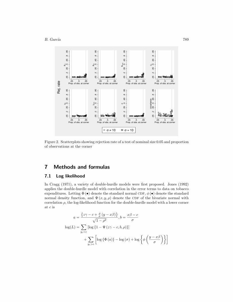
Figure 2 is analogous to figure 1. We note that tests on the covariance are particularlyunreliable, that the distinction between the cases where σ 6= 10 and σ = 10 seems notto matter, and that the rejection rate exceeds the nominal size of the test when theproportion of observations at the corner is around 0.9. However, when the proportionof observations at the corner is between 0.3 and 0.8, the sizes are mostly reliable withthe notable exception of tests of the covariance.
B. Garcıa 789
.05
.2.3
5.5
.65
.8.9
5Β
x1
.05 .5 .95Prop. of obs. at corner
.05
.2.3
5.5
.65
.8.9
5Β
d1
.05 .5 .95Prop. of obs. at corner
.05
.2.3
5.5
.65
.8.9
5Β
cons
.05 .5 .95Prop. of obs. at corner
.05
.2.3
5.5
.65
.8.9
5γ x
1
.05 .5 .95Prop. of obs. at corner
.05
.2.3
5.5
.65
.8.9
5γ d
1
.05 .5 .95Prop. of obs. at corner
.05
.2.3
5.5
.65
.8.9
5γ c
ons
.05 .5 .95Prop. of obs. at corner
.05
.2.3
5.5
.65
.8.9
5σ
.05 .5 .95Prop. of obs. at corner
.05
.2.3
5.5
.65
.8.9
5co
va
ria
nce
.05 .5 .95Prop. of obs. at corner
Re
j. r
ate
σ ≠ 10 σ = 10
Figure 2. Scatterplots showing rejection rate of a test of nominal size 0.05 and proportionof observations at the corner
7 Methods and formulas
7.1 Log likelihood
In Cragg (1971), a variety of double-hurdle models were first proposed. Jones (1992)applies the double-hurdle model with correlation in the error terms to data on tobaccoexpenditures. Letting Φ (•) denote the standard normal CDF, φ (•) denote the standardnormal density function, and Ψ (x, y, ρ) denote the CDF of the bivariate normal withcorrelation ρ, the log-likelihood function for the double-hurdle model with a lower cornerat c is
a =
{zγ − c+ ρ
σ (y − xβ)}
√1− ρ2
, b =xβ − c
σ
log(L) =∑
yi=c
[log {1−Ψ(zγ − c, b, ρ)}]
+∑
yi>c
[log {Φ(a)} − log (σ) + log
{φ
(y − xβ
σ
)}]

790 Double-hurdle model
If the upper corner is at c, then
log(L) =∑
yi=c
[log {1−Ψ(c− zγ,−b, ρ)}]
+∑
yi<c
[log {Φ(−a)} − log (σ) + log
{φ
(xβ − y
σ
)}]
7.2 Choosing the initial point
The optimization routine optimize() requires an initial point from which to initializethe optimization algorithm. My choice of starting point is [xβ, zγ, 0, 5]
′, where β are the
ordinary least-squares estimates of a regression of the dependent variable of the modelon x, the variables in the quantity equation; γ are the ordinary least-squares estimatesof a regression of the dependent variable of the model on z, the variables in the quantityequation; and ρ and σ are chosen to be 0 and 5, respectively.
There is no guarantee that the initial point will be feasible. If the initial point isinfeasible, the use of the from() option is recommended.
7.3 First derivatives
The first derivatives of the log likelihood (if βj is the constant, simply let xj = 1and likewise for γj) are given below. These were adapted from Jones and Yen (2000).Letting ψ (x, y, ρ) be the density of a bivariate normal with correlation ρ,

B. Garcıa 791
Ψ = Ψ(zγ − c, b, ρ)
ψ = Ψ(zγ − c, b, ρ)
Φ12 = Φ
(zγ − c− bρ√
1− ρ2
)
φ12 = Φ
(zγ − c− bρ√
1− ρ2
)
Φ21 = Φ
(b− ρ (zγ − c)√
1− ρ2
)
dβjd log (L)
=xjσ
[∑
y=c
{φ (b) Φ12
Ψ− 1
}+∑
y>c
{−ρφ (a)√1− ρ2Φ(a)
+y − xβ
σ
}]
dγjd log (L)
= zj
[∑
y=c
{φ (z − c) Φ21
Ψ− 1
}+∑
y>c
{φ (a)√
1− ρ2Φ(a)
}]
dσ12d log (L)
=1
σ
(∑
y=c
(ψ
Ψ− 1
)+∑
y>x
[y − xβ
σ
{φ (a)
Φ (a)√
1− ρ2
}+
aρ√1− ρ2
])
dσ
d log (L)=
1
σ
∑
y=c
[b
{Φ12φ (b)
1−Ψ
}+
ρψ
1−Ψ
]
+1
σ
∑
y>c
[(y − xβ
σ
)2
− 1 +
{−ρφ (a)
Φ (a)√1− ρ2
}(2y − xβ
σ+
aρ√1− ρ2
)]
The implementation of the derivatives for an upper corner at c requires a few minorchanges. First, the derivatives with respect to βj and γj should be multiplied by −1.Finally, multiply a, b, zγ − c, and (y − xβ)/σ by −1.
7.4 Weights
The weighting schemes implemented for dblhurdle are frequency weights (fw), sam-pling weights (pw), and importance weights (iw). Recall that the likelihood functionis summed over observations. To implement the weights, you need to multiply the ithterm of the summation over observations by the weight of the ith observation. Thefrequency weights are only allowed to be positive integers.

792 Double-hurdle model
When frequency weights are specified, the sample size is adjusted so that it is equalto the sum of the weights. The importance weights are allowed to be any real number.No sample-size adjustments are made when importance weights are specified. Thesampling weights are like the importance weights, but a robust estimator of the varianceis computed instead of the default oim estimator. No sample-size adjustment is madewhen sampling weights are specified, and the weights are not allowed to be negative.
Finally, analytic weights (aw) are not allowed. This command was written with thetobit command in mind. In that case, the aweights (normalized) divide the varianceof the error term. In the case of dblhurdle, the rationale for dividing the variance bythe normalized weights does not carry over well because we also have to estimate thecovariance between the error terms.
7.5 Prediction
There are three options in the prediction program that require some explanation. Theppar option computes the probability of being away from the corner conditional on thecovariates. Thus this option computes
Pr (y > c|x, z) = Φ
(zγ − c,
xβ − c
σ, ρ
)
The option ycond computes the following expectation:
E (y|x, z, y > c) =
∫ +∞
c
yf(y|u > c− zγ, ǫ > c− xβ)dy
f(y|u > c− zγ, ǫ > c− xβ) =
φ(
y−xβσ
)Φ
{zγ−c+ ρ
σ(y−xβ)√
1−ρ2
}
σΦ(zγ − c, xβ−c
σ , ρ)
Finally, the option yexpected computes the expected value of y conditional on xand z:
E (y|x, z) = c {1− Pr (y > c|x, z)}+ Pr (y > c|x, z)E (y|x, z, y > c)
Note that the options that involve integration are time consuming. Thus the optionstepnum() was added to the prediction program to allow the user some control of theexecution time for the integration. Letting ns denote the stepnum(), the step size ischosen to be
min(σ,√
1− ρ2)
ns
Execution is faster when the stepnum() is smaller, but the improved run time comesat a cost to accuracy. The default is stepnum(10).

B. Garcıa 793
When the corner is above, the expressions that change become
Pr (y < c|x, z) = Φ
(c− zγ,
c− xβ
σ, ρ
)
E (y|x, z, y < c) =
∫ c
−∞
yf(y|u < zγ − c, ǫ < xβ − c)dy
f(y|u < zγ − c, ǫ < xβ − c) =
φ(
xβ−yσ
)Φ
{c−zγ− ρ
σ(y−xβ)√
1−ρ2
}
σΦ(c− zγ, c−xβ
σ , ρ)
8 Conclusion
The double-hurdle model was an important contribution to the econometric toolkitused by researchers. I hope that readers will consider this model and, in particular, thedblhurdle command when their first instinct is to use the tobit model. The examplepresented in section 5 illustrates the flexibility of the model. It allows the researcher tobreak down the modeled quantity along two useful dimensions, the “quantity” dimensionand the “participation” dimension.
The command presented in this article only allows for a single corner in the data.One desirable feature to add is the capability to handle dependent variables with twocorners. Such variables are common (for example, 401k contributions), so this featurewould certainly provide higher value to users.
9 Acknowledgments
I wrote this article and the command described therein during a summer internship atStataCorp. It was exciting to meet the individuals behind Stata. I thank David Drukkerfor his support and for the time he spent going over the intricate details of the models.I also thank Rafal Raciborski for all of his comments, suggestions, and tips. Any errorsin my work are my own.
10 References
Cragg, J. G. 1971. Some statistical models for limited dependent variables with appli-cation to the demand for durable goods. Econometrica 39: 829–844.
Jones, A. M. 1992. A note on computation of the double-hurdle model with dependencewith an application to tobacco expenditure. Bulletin of Economic Research 44: 67–74.
Jones, A. M., and S. T. Yen. 2000. A Box-Cox double-hurdle model. Manchester School
68: 203–221.
Martınez-Espineira, R. 2006. A Box-Cox Double-Hurdle model of wildlife valuation:The citizen’s perspective. Ecological Economics 58: 192–208.

794 Double-hurdle model
Wooldridge, J. M. 2010. Econometric Analysis of Cross Section and Panel Data. 2nded. Cambridge, MA: MIT Press.
About the author
Bruno Garcıa is working toward a master’s degree in computational operations research at theCollege of William and Mary. He received his bachelor’s degree in applied mathematics andeconomics from Brown University.


![The Stata Journal ( Nonparametric Instrumental Variable ... · Abstract. This paper introduces Stata commands [R] npiv and [R] npivcv, which implement nonparametric instrumental variable](https://img.pdfslide.us/doc/110x75/5e916f7be5514b028458428f/the-stata-journal-nonparametric-instrumental-variable-abstract-this-paper.jpg)