The Stata Journal - AgEcon Searchageconsearch.umn.edu/bitstream/229441/2/sjart_st0272.pdf · The purpose of the Stata Journal is to promote free communication among Stata users. The

The Stata Journal

Editors

H. Joseph Newton

Department of Statistics

Texas A&M University

College Station, Texas

[email protected]

Nicholas J. Cox

Department of Geography

Durham University

Durham, UK

[email protected]

Associate Editors

Christopher F. Baum, Boston College

Nathaniel Beck, New York University

Rino Bellocco, Karolinska Institutet, Sweden, and

University of Milano-Bicocca, Italy

Maarten L. Buis, WZB, Germany

A. Colin Cameron, University of California–Davis

Mario A. Cleves, University of Arkansas for

Medical Sciences

William D. Dupont, Vanderbilt University

Philip Ender, University of California–Los Angeles

David Epstein, Columbia University

Allan Gregory, Queen’s University

James Hardin, University of South Carolina

Ben Jann, University of Bern, Switzerland

Stephen Jenkins, London School of Economics and

Political Science

Ulrich Kohler, WZB, Germany

Frauke Kreuter, Univ. of Maryland–College Park

Peter A. Lachenbruch, Oregon State University

Jens Lauritsen, Odense University Hospital

Stanley Lemeshow, Ohio State University

J. Scott Long, Indiana University

Roger Newson, Imperial College, London

Austin Nichols, Urban Institute, Washington DC

Marcello Pagano, Harvard School of Public Health

Sophia Rabe-Hesketh, Univ. of California–Berkeley

J. Patrick Royston, MRC Clinical Trials Unit,

London

Philip Ryan, University of Adelaide

Mark E. Schaffer, Heriot-Watt Univ., Edinburgh

Jeroen Weesie, Utrecht University

Nicholas J. G. Winter, University of Virginia

Jeffrey Wooldridge, Michigan State University

Stata Press Editorial Manager

Lisa Gilmore

Stata Press Copy Editors

David Culwell and Deirdre Skaggs

The Stata Journal publishes reviewed papers together with shorter notes or comments, regular columns, book

reviews, and other material of interest to Stata users. Examples of the types of papers include 1) expository

papers that link the use of Stata commands or programs to associated principles, such as those that will serve

as tutorials for users first encountering a new field of statistics or a major new technique; 2) papers that go

“beyond the Stata manual” in explaining key features or uses of Stata that are of interest to intermediate

or advanced users of Stata; 3) papers that discuss new commands or Stata programs of interest either to

a wide spectrum of users (e.g., in data management or graphics) or to some large segment of Stata users

(e.g., in survey statistics, survival analysis, panel analysis, or limited dependent variable modeling); 4) papers

analyzing the statistical properties of new or existing estimators and tests in Stata; 5) papers that could

be of interest or usefulness to researchers, especially in fields that are of practical importance but are not

often included in texts or other journals, such as the use of Stata in managing datasets, especially large

datasets, with advice from hard-won experience; and 6) papers of interest to those who teach, including Stata

with topics such as extended examples of techniques and interpretation of results, simulations of statistical

concepts, and overviews of subject areas.

The Stata Journal is indexed and abstracted by CompuMath Citation Index, Current Contents/Social and Behav-

ioral Sciences, RePEc: Research Papers in Economics, Science Citation Index Expanded (also known as SciSearch,

Scopus, and Social Sciences Citation Index.

For more information on the Stata Journal, including information for authors, see the webpage

http://www.stata-journal.com

http://www.stata-journal.com

Subscriptions are available from StataCorp, 4905 Lakeway Drive, College Station, Texas 77845, telephone

979-696-4600 or 800-STATA-PC, fax 979-696-4601, or online at

http://www.stata.com/bookstore/sj.html

Subscription rates listed below include both a printed and an electronic copy unless otherwise mentioned.

U.S. and Canada Elsewhere

1-year subscription $ 79 1-year subscription $115

2-year subscription $155 2-year subscription $225

3-year subscription $225 3-year subscription $329

3-year subscription (electronic only) $210 3-year subscription (electronic only) $210

1-year student subscription $ 48 1-year student subscription $ 79

1-year university library subscription $ 99 1-year university library subscription $135

2-year university library subscription $195 2-year university library subscription $265

3-year university library subscription $289 3-year university library subscription $395

1-year institutional subscription $225 1-year institutional subscription $259



Back issues of the Stata Journal may be ordered online at

http://www.stata.com/bookstore/sjj.html

Individual articles three or more years old may be accessed online without charge. More recent articles may

be ordered online.

http://www.stata-journal.com/archives.html

The Stata Journal is published quarterly by the Stata Press, College Station, Texas, USA.

Address changes should be sent to the Stata Journal, StataCorp, 4905 Lakeway Drive, College Station, TX

77845, USA, or emailed to [email protected].

®

Copyright c© 2012 by StataCorp LP

Copyright Statement: The Stata Journal and the contents of the supporting files (programs, datasets, and

help files) are copyright c© by StataCorp LP. The contents of the supporting files (programs, datasets, and

help files) may be copied or reproduced by any means whatsoever, in whole or in part, as long as any copy

or reproduction includes attribution to both (1) the author and (2) the Stata Journal.

The articles appearing in the Stata Journal may be copied or reproduced as printed copies, in whole or in part,

as long as any copy or reproduction includes attribution to both (1) the author and (2) the Stata Journal.

Written permission must be obtained from StataCorp if you wish to make electronic copies of the insertions.

This precludes placing electronic copies of the Stata Journal, in whole or in part, on publicly accessible websites,

fileservers, or other locations where the copy may be accessed by anyone other than the subscriber.

Users of any of the software, ideas, data, or other materials published in the Stata Journal or the supporting

files understand that such use is made without warranty of any kind, by either the Stata Journal, the author,

or StataCorp. In particular, there is no warranty of fitness of purpose or merchantability, nor for special,

incidental, or consequential damages such as loss of profits. The purpose of the Stata Journal is to promote

free communication among Stata users.

The Stata Journal (ISSN 1536-867X) is a publication of Stata Press. Stata, , Stata Press, Mata, ,

and NetCourse are registered trademarks of StataCorp LP.

http://www.stata.com/bookstore/sj.html

http://www.stata.com/bookstore/sjj.html

http://www.stata-journal.com/archives.html

The Stata Journal (2012)12, Number 3, pp. 515–542

Long-run covariance and its applications in

cointegration regression

Qunyong WangInstitute of Statistics and Econometrics

Nankai UniversityTianjin, China

[email protected]

Na WuEconomics School

Tianjin University of Finance and EconomicsTianjin, China

Abstract. Long-run covariance plays a major role in much of time-series inference,such as heteroskedasticity- and autocorrelation-consistent standard errors, gener-alized method of moments estimation, and cointegration regression. We propose aStata command, lrcov, to compute long-run covariance with a prewhitening strat-egy and various kernel functions. We illustrate how long-run covariance matrixestimation can be used to obtain heteroskedasticity- and autocorrelation-consistentstandard errors via the new hacreg command; we also illustrate cointegration re-gression with the new cointreg command. hacreg has several improvements com-pared with the official newey command, such as more kernel functions, automaticdetermination of the lag order, and prewhitening of the data. cointreg enables theestimation of cointegration regression using fully modified ordinary least squares,dynamic ordinary least squares, and canonical cointegration regression methods.We use several classical examples to demonstrate the use of these commands.

Keywords: st0272, lrcov, hacreg, cointreg, long-run covariance, fully modified or-dinary least squares, dynamic ordinary least squares, canonical cointegration re-gression

1 Introduction

Long-run covariance (LRCOV) plays a major role in much of time-series inference, such asheteroskedasticity- and autocorrelation-consistent (HAC) standard errors, efficient gener-alized method of moments (GMM) estimation, cointegration regression, etc. Asymptotictheory for estimators has developed rapidly within the literature, primarily focused onthe LRCOV. Practical applications of robust inference that take into account poten-tial heteroskedasticity and autocorrelation of unknown forms in the data involve LRCOV

matrix estimation, such as White heteroskedasticity robust standard errors and Newey–West HAC standard errors.

Unit-root tests and cointegration tests are now routinely used in empirical research.LRCOV has been widely applied to nonstationary time-series analysis, such as the

c© 2012 StataCorp LP st0272

516 Long-run covariance and its applications in cointegration regression

Phillips–Perron unit-root test (Phillips and Perron 1988), cointegration tests (Marmoland Velasco 2004) and panel cointegration tests (Pedroni 2004), a model’s stabilitybased on fully modified ordinary least squares (FMOLS) (Hansen 1992), canonical cor-relation regression (CCR) with both I(1) and I(2) variables (Choi, Park, and Yu 1997),fully modified value at risk (VAR), and fully modified GMM estimation (Quintos 1998).

Three approaches are popular for computing LRCOV: the nonparametric kernel meth-od, the parametric method, and the prewhitened kernel method. The kernel methodhas a long history for which the kernel and bandwidth are two important determinantsof the finite-sample properties of LRCOV. Many kernels have been proposed (Priestley1981), among which the Bartlett, Parzen, and quadratic spectral may be the mostpopular choices. Some new kernels have been proposed recently, such as the class ofsteep-origin kernels of Phillips, Sun, and Jin (2007).

To date, there are two widely used formulas for selecting the bandwidth, proposedin Andrews (1991) and Newey and West (1994). Hirukawa (2010) proposed an alter-native approach, namely, the two-stage plug-in bandwidth selection approach. For theparametric approach, econometric models are used to prewhiten the data; these mod-els include the VAR prewhitening of den Haan and Levin (1997) and the autoregressivemoving-average (ARMA) prewhitening of Lee and Phillips (1994). The prewhitened ker-nel method (Andrews and Monahan 1992) combines the parametric method and thenonparametric kernel method. All three approaches will be discussed in section 2.

Some software is able to compute LRCOV and fit some relevant models with itsapplications (software such as EViews, Rats, and the Coint package of Gauss). Thetime-series utilities of Stata have increased rapidly. Some existing Stata commandsestimate LRCOV implicitly (newey, ivreg2, etc.), but there is still no explicit commandavailable.

In this article, we offer the lrcov command for computing the symmetric and one-sided LRCOV in Stata. The lrcov program supports Andrews (1991) and Newey andWest (1994) automatic bandwidth selection methods for kernel estimators, as well asinformation criteria–based lag-length selection methods for value-at-risk HAC (VARHAC)and prewhitening estimation. We also provide two additional commands, hacreg andcointreg, as applications of lrcov. hacreg estimates HAC standard error and extendsStata’s official newey command in some ways. cointreg estimates FMOLS, dynamicordinary least squares (DOLS), and CCR.

The remainder of the article is organized as follows. The background of LRCOV

is introduced in section 2. In section 3, we introduce the syntax of lrcov and itsapplications in the calculation of HAC standard error and GMM estimation. hacreg andcointreg are illustrated in sections 4 and 5. In section 6, we draw conclusions andoutline future research.

Q. Wang and N. Wu 517

2 Background of LRCOV

For second-order stationary processes, the long-run variance is defined as the sum of allautocovariances or, equivalently, in terms of the spectrum at frequency zero. Considera sequence of mean-zero random p-vectors, vt(θ), that have K parameters. The LRCOV

matrix Ω of vt(θ) is

Ω =

∞∑

j=−∞Γj

Γj = E(vtv′t−j), j ≥ 0

Γj = Γ′−j , j < 0

where Γj is the autocovariance matrix of vt at lag j. Define the one-sided LRCOV Λ0

and strict one-sided LRCOV Λ1 as

Λ0 =∞∑

j=0

Γj = Λ1 + Γ0

Λ1 =

∞∑

j=1

Γj

where Γ0 is the contemporaneous covariance. So the symmetric two-sided LRCOV canalso be written as

Ω = Λ1 +Λ1′ + Γ0 = Λ0 +Λ0

′ − Γ0

Given the definition of Ω =∑∞

j=−∞ Γj , it is natural to estimate Ω using the sample

autocovariances, Γj = T−1∑T

t=j+1 vtv′t−j , as estimates of their population analogs.

This leads to the one-sided estimator

Ω = Γ0 +∑K

j=1Γj

White and Domowitz (1984) first proposed this type of estimator and showed its

consistency. While Ω converges in probability to a positive-definite matrix, it maybe indefinite in finite samples. As argued by Hall (2005), the source of the troublelies in the weights given to the sample autocovariances. The solution is to construct anestimator in which the contributions of the sample autocovariance matrices are weightedto downgrade their role sufficiently in finite samples to ensure positive semidefiniteness;however, the weights also need to tend to one as T → ∞ to ensure consistency. Thisis the intuition behind the nonparametric kernel approach of HAC matrices (Andrews1991; Newey and West 1987). The nonparametric kernel approach estimates the LRCOV

by taking a weighted sum of the sample autocovariances of the observed data

Ω = Γ0 +∑K

j=1k(j)Γj


where k(j) is known as the kernel (or weight). The kernel must be chosen to ensure thetwin properties of consistency and positive semidefiniteness.

Below we will discuss the nonparametric kernel method and two other methods toestimate Ω, that is, the parametric VARHAC approach (den Haan and Levin 1997) andthe prewhitened kernel approach (Andrews and Monahan 1992).

2.1 Nonparametric kernel method

The class of kernel HAC covariance matrix estimators in Andrews (1991) may be writtenas

Ω =T

T −K

∞∑

j=−∞k(j/bT )Γj

Γj =1

T

T∑

t=j+1

vtv′t−j , j ≥ 0

Γj = Γ′−j , j < 0

(1)

k is a symmetric kernel (or lag window) function that is continuous at the originand satisfies k(x) ≤ 1 and k(0) = 1. The allowed kernels in lrcov are listed in table 1.Candidate kernel functions can be found in standard texts, for example, Brillinger (1980)and Priestley (1981). bT is the bandwidth parameter, which depends on the numberof observations. bT controls the number of autocovariances included in the LRCOV

estimator for some kernels, such as the Bartlett and Parzen kernels. T/(T −K) is anoptional correction of degrees of freedom associated with the parameters in the model.So the nonparametric kernel estimator can be viewed as a weighted average of sampleautocovariances. The weights are just values of the lag window function evaluated atdifferent lag lengths.

Andrews (1991) shows that the quadratic spectral weights are optimal in the sensethat they minimize an asymptotic mean-squared-error criterion for the estimation ofLRCOV. His results imply that this choice only marginally dominates the Parzen weights,but Parzen and quadratic spectral weights should be much better than the Bartlettweights. However, neither dominates the Bartlett weight to the extent predicted bythe theory. Newey and West (1994) conclude that the choice between the kernels is notparticularly important and the bandwidth is a much more important determinant ofthe finite-sample properties of LRCOV. For consistency, bT must tend to infinity with T .Andrews (1991) shows that the asymptotic mean squared error is minimized by settingbT equal to O(T 1/3) for the Bartlett weights and equal to O(T 1/5) for both the Parzenand quadratic spectral weights. However, this type of condition provides little practicalguidance.


Table 1. Kernel function properties

Kernel Function ck q rate

Bartlett k(x) =

1− |x| if x ≤ 1.0

0 otherwise1.1447 1 2/9

Bohman k(x) =

(1− |x|) cos(πx) +

sin(π|x|)π

if x ≤ 1.0

0 otherwise2.4202 2 4/25

Daniell k(x) = sin(πx)/(πx) 0.4462 2 –

Parzen k(x) =

1− 6x2(1− |x|) if 0 ≤ |x| ≤ 0.5

2(1− |x|)3 if 0.5 < |x| ≤ 1.0

0 otherwise

2.6614 2 4/25

Parzen–Riesz k(x) =

1− x2 if x ≤ 1.0

0 otherwise1.1340 2 4/25

Parzen–Geometric k(x) =

1/(1 + |x|) if x ≤ 1.0

0 otherwise1.0000 1 2/9

Parzen–Cauchy k(x) =

1/(1 + x2) if x ≤ 1.0

0 otherwise1.0924 2 4/25

Quadratic spectral k(x) = 2512π2x2

sin(1.2πx)

1.2πx− cos(1.2πx)

1.3221 2 2/25

Tukey–Hamming k(x) =

0.54 + 0.46 cos(πx) if x ≤ 1.0

0 otherwise1.6694 2 4/25

Tukey–Hanning k(x) =

0.50 + 0.50 cos(πx) if x ≤ 1.0

0 otherwise1.7462 2 4/25

Tukey–Parzen k(x) =

0.436 + 0.564 cos(πx) if x ≤ 1.0

0 otherwise1.8576 2 4/25

Truncated uniform k(x) =

1 if |x| ≤ 1.0

0 otherwise0.6611 1/5 –

Note: ck and q are used to compute optimal bandwidth; rate is the optimal rate of increase for thelag selection in Newey and West (1987).

Andrews (1991) and Newey and West (1994) offer two automatic bandwidth selec-tion techniques based on observations to estimating bT . Both methods estimate bTaccording to the following rule

bT = ckα(q)T1/(2q+1)

where ck and q depend on the type of kernel function and are also listed in table 1.The Andrews (1991) method estimates bT parametrically by fitting a simple parametric


time-series model to the original data, and then deriving the autocovariances and cor-responding α(q). For the univariate autoregressive AR(1) models corresponding to thep variables,

α(q) =

∑ps=1 ws

(fqs

)2

∑ps=1 ws

(f0s

)2

fqs =1

2π

∑∞

j=−∞|j|qΓs,j

(2)

where Γs,j are the estimated autocovariances at lag j implied by the univariate AR(1)

specification for the sth variable. ws is the weight for the sth variable. Andrews (1991)suggests using either ws = 1 for all or for all but the instrument corresponding to theintercept in regression settings. However, to date, no further guidance is available abouthow this choice should be made or its impact on the finite-sample properties of LRCOV.

Newey and West (1994) use a nonparametric approach. First, define the scalar au-tocovariance estimators

σj =1

T

T∑

t=j+1

w′vtv′t−jw = w′Γjw (3)

where w = (w1, w2, . . . , wp)′. Then compute nonparametric truncated kernel estimators

of the Parzen measures of smoothness:

fqs =1

2π

∑n

j=−n|j|qσj (4)

The Newey and West (1994) estimator for α(q) is

α(q) =(fq/f0

)2

Kiefer and Vogelsang (2002a,b) proposed the use of inconsistent HAC estimates basedon conventional kernels but with the bandwidth set equal to the sample size. They showthat such estimates lead to asymptotically valid tests that can have better finite-sample-size properties than tests based on consistent HAC estimates. Their power analysisand simulations reveal that the Bartlett kernel produces the highest power function inregression testing with bT = T , although power is noticeably less than what can beattained using conventional procedures involving consistent HAC estimators.

2.2 Parametric VARHAC method

One of the mechanisms that can improve covariance matrix estimates is derived from theidea of prewhitening. Prewhitening has a long history in time-series analysis. Recently,


it has also been applied to the estimation of LRCOV. The stated idea of prewhiteningis as follows. One first prefilters the original data to obtain a less dependent seriesthat has a flatter spectrum. The spectral density function of the filtered data can thenbe estimated with less bias and recolored to produce an estimator for the spectrum ofthe original series with reduced bias. If the true data-generating process belongs tothe parametric class that is used for prewhitening, then the parametric prewhitenedestimator has improved the convergence rate.

den Haan and Levin (1997) proposed the VARHAC parametric method to estimateLRCOV. They first whiten the data using the VAR(q) model and compute the contem-poraneous covariance for the whitened data. They then recolor it to the original data.

Let the filtered data be

v∗t = vt −

∑q

j=1Ajvt−j

with contemporaneous covariance

Γ∗0 =

1

T − q

∑T

t=q+1v∗tv

∗t′

The two-sided LRCOV is

Ω =T − q

T − q −KDΓ

∗0D

D =(Ip −

∑q

j=1Aj

)−1

where Γ∗0 is the contemporaneous covariance of v∗

t . den Haan and Levin (1996) recom-mend choosing the lag length via a model-selection criterion. Their theoretical analysissuggests that the Bayesian information criterion is a better choice than Akaike’s infor-mation criterion (AIC); however, their simulation evidence suggests that the two criteria

perform comparably in this context. den Haan and Levin (1996) show that Ω is con-sistent provided that q → ∞ as T → ∞ and q = O(T 1/3).

The VARHAC estimators for the one-sided LRCOV, Λ0 and Λ1, do not have simple

expressions in terms of A and Γ∗0. For the VAR(1) model, the one-sided LRCOV may be

written as (QMS 2010)

Λ0 =T − q

T − q −K

(Ip − A1

)−1

Γ0

Λ1 =T − q

T − q −KA1

(Ip − A1

)−1

Γ0

where Γ0 can be computed using (1).


2.3 Prewhitened kernel method

The prewhitened kernel approach is a hybrid method that combines the parametricmethod and the nonparametric kernel method. The prewhitened method uses a para-metric model to obtain residuals that prefilter the data and a nonparametric kernelestimator to obtain an LRCOV estimator of the whitened data. Andrews and Monahan(1992) proposed a VAR prewhitening procedure for the estimation of the covariance ma-trix. Lee and Phillips (1994) used the Hannan–Rissanen recursive estimation procedureand order-selection methods and proposed an ARMA prewhitened long-run variance esti-mator. All of these prewhitened estimators use parametric (AR or ARMA) prewhiteningprocedures in the time domain. The resulting prewhitened LRCOV estimate is thenrecolored to undo the effects of the transformation.

To estimate LRCOV using the method of Andrews and Monahan (1992), we firstfilter the data using VAR(q). We then construct the innovation’s kernel LRCOV using(1). The formula of one-sided LRCOV for VAR(1) was given in Hansen (1992):

Λ0 = DΛ∗0D

′ + DA1Γ0

The one-sided LRCOV for the VAR(q) model is derived by Park and Ogaki (1991):

Λ1 = DΛ∗1D

′ + D∑q−1

j=0

∑q

i=j+1AiΓj

The VARHAC method is advantageous because the LRCOV can be estimated straight-forwardly from the model. den Haan and Levin (2000) found that once data-dependentVAR prewhitening has been used in linear regression, the effect of the prewhitenedkernel method is negligible or even counterproductive. The potential disadvantage isthat if the model is incorrect, then the LRCOV estimator is inconsistent. The closerthe prewhitened model is to the true model, the less bias in the estimator. Indeed,Andrews and Monahan (1992) exhibit examples where the mean squared error can ac-tually be worse than that of the standard estimator. Sul, Phillips, and Choi (2005)showed that the small-sample bias in the estimation of autoregressive coefficients istransmitted to the recoloring filter, leading to HAC variance estimates that can be badlybiased. They recommended using recursive demeaning procedures to mitigate the effectsof small-sample autoregressive bias.

For the kernel method, the LRCOV estimator is consistent under much weaker condi-tions than the VARHAC method. Unfortunately, these more general estimators can ex-hibit poor finite-sample performance, which prompted the construction of prewhitenedkernel estimator.

As argued by Andrews and Monahan (1992) and Lee and Phillips (1994), the pre-whitened kernel estimator of the LRCOV reduces bias and improves the rate of conver-gence of existing estimators. Simulation evidence in Newey and West (1994) suggeststhat the use of prewhitening and recoloring improves the finite-sample performance ofthe parameters’ asymptotic confidence intervals. Xiao and Oliver (2002) proposed a


nonparametric spectral density estimator for time-series models with general autocor-relation. Their simulation study showed that the prewhitened kernel estimator reducesbias and mean squared error in spectral density estimation. Christou and Pittis (2002)conducted a Monte Carlo study to investigate the finite-sample properties in the FMOLS

procedure. Their results suggest that the prewhitened kernel estimator minimizes thesecond-order asymptotic bias effects in cointegration regression.

In our Stata lrcov and cointreg commands, the default specification is the non-parametric kernel method. Users can choose to prewhiten the data or not.

3 lrcov: Stata command to compute LRCOV

lrcov computes LRCOV in Mata. For the prewhitened kernel method, matrix inversionis required. lrcov uses the invsym and pinv commands.

3.1 Syntax

lrcov varlist[if] [

in] [

, wvar(varname) nocenter constant dof(#)

vic(string) vlag(#) kernel(string) bwidth(#) bmeth(string) blag(#)

bweig(numlist) bwmax(#) btrunc disp(string)]

varlist may contain factor variables or time-series operators.

3.2 Options

wvar(varname) specifies the weight of the observation; that is, multiply each variablein varlist with varname.

nocenter requests that lrcov not center the data before computing. By default, lrcovcenters the data using the mean before computing LRCOV.

constant adds constant to varlist. This option may only be used with the wvar()

option.

dof(#) adjusts the LRCOV by degrees of freedom. The default is dof(0).

vic(string) specifies the information criteria to select the optimal lags in VAR. aic,bic, and hq are allowed. To prewhiten the data, both vic() and vlag() must bespecified.

vlag(#) specifies the maximum lag to select the optimal lag length if the vic() optionis specified. Otherwise, # is the lag order of the VAR model to estimate. If theuser specified vic() but not vlag(), lrcov automatically sets the maximum lag toint(T 1/3). To prewhiten the data, both vic() and vlag() must be specified.


kernel(string) specifies the type of kernel function. string may be none, bartlett,bohman, daniell, parzen, qs, priesz, pcauchy, pgeometric, thamming, thanning,or tparzen. If the user specifies kernel(none), the bwidth(), bmeth(), blag(),bweig(), and btrunc options will be ignored.

bwidth(#) specifies the bandwidth by hand. If this option is specified, the programwill ignore the bmeth(), blag(), bweig(), and btrunc options.

bmeth(string) specifies the bandwidth selection procedure, including nwfixed [Newey–West fixed lag, that is, 4 × (T/100)2/9], andrews, and neweywest. The default isbmeth(nwfixed).

blag(#) specifies the parameter of n in bandwidth selection (4). If this option is notspecified, the program will set it based on 20(n/100)r, where (x) means the largestinteger less than x and r depends on the kernel function.

bweig(numlist) specifies the weight vector w when automatically computing the band-width according to (2) and (3). The number of elements in numlist should be equalto the number of variables in varlist. The default weight is 1 for all variables.

bwmax(#) specifies the maximum bandwidth. If the bandwidth supplied by the user orautomatically determined by the procedure is greater than #, then lrcov will use# as the bandwidth.

btrunc truncates the bandwidth to an integer.

disp(string) requests that lrcov display the detailed results, including two (two-sidedLRCOV), one (one-sided LRCOV), sone (strict one-sided LRCOV), and cont (contem-poraneous covariance). The default is disp(two).

3.3 Saved results

lrcov saves the following in r():

Scalarsr(bwidth) bandwidth b(vlag) lag of VAR model

Macrosr(kernel) kernel function r(vic) type of information criterionr(bmeth) automatic bandwidth method

Matricesr(Omega) two-sided LRCOV r(Omega0) contemporaneous covariancer(Omegaone) one-sided LRCOV (lag) r(Omegasone) strict one-sided LRCOV (lag)

3.4 Examples

We use the macroeconomic data downloaded from Stata’s official website to illustratethe use of lrcov. The data include macroeconomic indicators of industrial productionindex, ipman; an aggregate weekly hours index, hours; aggregate unemployment, unemp;and real disposable income, income.


. webuse dfex(St. Louis Fed (FRED) macro data)

. describe

Contains data from http://www.stata-press.com/data/r12/dfex.dtaobs: 443 St. Louis Fed (FRED) macro datavars: 6 14 May 2011 17:59size: 19,492

storage display valuevariable name type format label variable label

month float %tm Monthunemp double %10.0g Civilian unemployment ratehours double %10.0g Aggregate weekly hours worked

index: total private industriesinc96 double %10.0g Real disposable personal incomeipman double %10.0g Industrial production;

manufacturing (NAICS)income double %10.0g Real disposable income (100´s)

Sorted by: month

Examples of different specifications

We assume the variables are I(1), so we compute the LRCOV of the differenced seriesdirectly.

Default case: Bartlett kernel. No prewhitening, Newey–West automatic bandwidthselection.

. lrcov d.(ipman income hours unemp)

Long Run Covariance:

VAR Pre-whitening = noKernel type = BartlettBandwidth (Newey-West) = 16.896Dof adjustment = 0

D. D. D. D.Two-sided ipman income hours unemp

D.ipman .9930469 .1527449 .5334321 -.2557916D.income .1527449 .0889101 .0795833 -.0443571D.hours .5334321 .0795833 .3991929 -.1804581D.unemp -.2557916 -.0443571 -.1804581 .0967915

The header consists of VAR Pre-whitening (or it could have VAR Lag and the in-formation criterion: AIC, Bayesian, or Hannan and Quinn), Kernel type, Bandwidthand its automatic selection method (Andrews, Newey–West, or N–W fixed), and Dof

adjustment. The row title of the matrix depends on the specification of the disp()

option (disp(two) by default).


Case 2: Nonparametric kernel approach. Quadratic spectral kernel, fixed bandwidthat 10.

. lrcov d.(ipman income hours unemp), kernel(qs) bwidth(10)


VAR Pre-whitening = noKernel type = Quadratic SpectralBandwidth (user) = 10Dof adjustment = 0



Case 3: Parametric approach. VARHAC estimation using VAR(1).

. lrcov d.(ipman income hours unemp), vlag(1) kernel(none)


Var lag (user) = 1Kernel type = NoneDof adjustment = 0



Case 4: Prewhitened kernel approach. Prewhiten using VAR(1), Parzen kernel, andAndrews automatic bandwidth.

. lrcov d.(ipman income hours unemp), vlag(1) kernel(parzen) bmeth(andrews)


Var lag (user) = 1Kernel type = ParzenBandwidth (Andrews) = 3.8986Dof adjustment = 0




Case 5: More flexible options. Prewhiten using VAR with lag selected by AIC,quadratic spectral kernel, Newey–West automatic bandwidth with truncated lag = 10.

. lrcov d.(ipman income hours unemp), vic(aic) kernel(qs) bmeth(neweywest)> blag(10)


Var lag (AIC) = 7Kernel type = Quadratic SpectralBandwidth (Newey-West) = 11.958Dof adjustment = 0


D.ipman 1.47109 .2149076 .8322045 -.4151169D.income .2149076 .0898623 .1285044 -.0700764D.hours .8322045 .1285044 .6190196 -.2999706D.unemp -.4151169 -.0700764 -.2999706 .1593269

Using lrcov to compute HAC variance

Next we use lrcov to compute the robust covariance matrix in linear regression, y =Xβ+u,Var(u) = Ω. The ordinary least squares (OLS) estimators are β = (X′X)−1X′y,

and their covariance is Cov(β)= (X′X)−1(X′ΩX)(X′X)−1. We assume the equation

to be arbitrarily specified as

∆ipmant = β0 + β1∆incomet + β2∆hourst + β3∆unempt + ut

The HAC covariance matrix is computed as follows:

. quietly regress d.ipman d.(income hours unemp)

. quietly predict u, res

. quietly lrcov d.(income hours unemp), wvar(u) constant dof(4) kernel(none)

. matrix covu = r(Omega)

. matrix accum xx = d.(income hours unemp)(obs=442)

. matrix xxi = invsym(xx)

. matrix cov = 442*xxi*covu*xxi

. matlist cov

D. D. D.income hours unemp _cons

D.income .0021644 -.0005001 .0006004 1.16e-06D.hours -.0005001 .0051949 .0021574 -.0011289D.unemp .0006004 .0021574 .014977 -.000245

_cons 1.16e-06 -.0011289 -.000245 .0006414


In fact, the hacreg command described below computes the robust covariance matrixin just the same way. The same results can be obtained using the following Statacommands:

. quietly regress d.ipman d.(income hours unemp), vce(robust)

. matlist e(b)

(output omitted )

. matlist e(V)

(output omitted )

Using lrcov to perform GMM estimation

Similar computation is easily applied to GMM estimation. The GMM estimator and itsvariance are

βGMM = (X′ZWZ′X)−1X′ZWZ′y

Cov(βGMM

)= n(X′ZWZ′X)−1X′WSWZ′X(X′ZWZ′X)−1

where X are explanatory variables and Z are instrumental variables. S, the estimatorof E(ziuiuiz

′i), is calculated using the residuals based on βGMM. The weight matrix

W = (Z′ΩZ)−1 is calculated using the residuals from the initial two-stage least-squares

estimates. If we set W = S−1, then we obtain the optimal two-step GMM estimator,

and the covariance matrix reduces to Cov(βGMM

)= n(X′ZWZ′X)−1. The following

commands estimate the two-step GMM estimator using the lrcov command:

. * one-step GMM (two-stage least squares)

. qui ivregress 2sls d.ipman d.income (d.hours d.unemp = DL(1/2).(hours unemp))

. qui predict u, residuals

. * weighted matrix using long run variance

. local inst = "d.income DL(1/2).(hours unemp)"

. qui lrcov ìnst´, nocenter wvar(u) constant kernel(bartlett) bwidth(11)

. matrix w = r(Omega)

. * two-step GMM estimator

. qui matrix accum xz = d.hours d.unemp d.income ìnst´

. matrix xz = xz[1..3, 4...] \ xz["_cons", 4...]

. matrix accum yz = d.ipman ìnst´(obs=440)

. matrix yz = yz[1, 2...]

. matrix b = invsym(xz*invsym(w)*xz´)*(xz*invsym(w)*yz´)

. matrix V = 440*invsym(xz*invsym(w)*xz´)

. matlist b´

D. D. D.hours unemp income _cons

D.ipman .5323454 -1.933122 -.0445388 .1229558


. matlist V

D. D. D.hours unemp income _cons

D.hours .0189107D.unemp .0066483 .1128266

D.income .0010752 -.0003729 .0027054_cons -.0025717 -.0001957 -.0003734 .0009218

The same results can be obtained using the ivregress command.1

. qui ivregress gmm d.ipman d.income (d.hours d.unemp = DL(1/2).(hours unemp)),> vce(unadjusted) wmatrix(hac bartlett 10)

. matlist e(b)

(output omitted )

. matlist e(V)

(output omitted )

Note that in the Bartlett (Parzen, Parzen–Riesz, etc.) kernels, k(1) = 0 andceil(bT ) − 1 autocovariances enter the estimator with nonzero weights where ceil(x)denotes the largest integer that is smaller than or equal to x. So the truncation param-eter 10 in ivregress is equivalent to bwidth(11) in lrcov.

4 hacreg: HAC standard errors in linear regression

We provide the hacreg command to implement the HAC-type standard errors. hacreghas several improvements over the official Stata newey command. hacreg can auto-matically determine the optimal lag based on information criteria. Moreover, hacregallows more-flexible treatment with LRCOV, such as prewhitening the data and morekernel functions.

4.1 Syntax

hacreg depvar indepvars[if] [

in] [

, noconstant level(#) lrcov options]

depvar may contain time-series operators. indepvars may contain factor variables andtime-series operators. by is allowed.

1. As pointed out by StataCorp (2009), many software packages that implement GMM estimationuse the heteroskedasticity-consistent weighting matrix to obtain the optimal two-step estimatesbut do not use a heteroskedasticity-consistent variance, even though they may label the standarderrors as being robust. To replicate results obtained from other packages, you may have to use thevce(unadjusted) option.


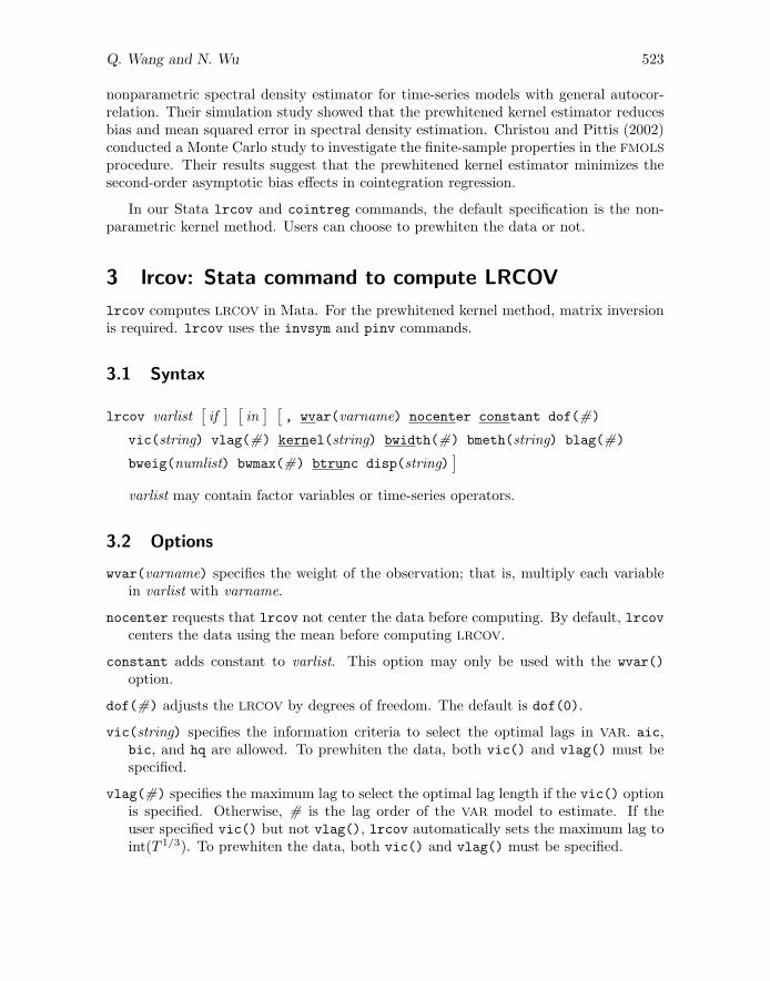
4.2 Options

noconstant suppresses the constant in the regression equation.

level(#) sets the confidence level; default is level(95).

lrcov options specifies the options to compute LRCOV, which include kernel(string),vlag(#), vic(string), bwidth(#), bmeth(string), blag(#), and btrunc. All ofthese options are specified in the same way as for the lrcov command described insection 3.2.

4.3 Saved results

hacreg saves the following in e():

Scalarse(N) number of observations e(df m) model degrees of freedome(r2) R-squared e(ll) log likelihoode(r2 a) adjusted R-squared e(ll 0) log likelihood, constant-onlye(rank) rank of e(V) modele(rss) residual sum of squares e(mss) residual sum of squarese(rmse) root of mean squared error e(F) model F statistice(df r) residual degrees of freedom

Macrose(cmd) hacreg e(vcetype) type of covariancee(cmdline) command as typed e(title) title of regressione(depvar) name of dependent variable e(properties) b Ve(predict) program to implement predict

Matricese(b) coefficient vector e(V) variance–covariance matrix of

the estimators

Functionse(sample) marks estimation sample

4.4 Example: Dynamic impact of cold weather on orange juice price

Stock and Watson (2006) discussed the effect of cold weather on the price change oforange juice using the HAC standard error. The model was specified as

dlnpojt = β0 +18∑

l=1

βlFDDt−l + ut

where dlnpoj is the price change computed as differencing the log series. FDD is thenumber of freezing degree days. The βl reflects the dynamic multiplier at lag l. Theaccumulated dynamic multiplier at lag l can be estimated by the model

dlnpojt = β0 +

17∑

l=1

βl∆FDDt−l + β18FDDt−18 + ut


The data are downloadable from Stock and Watson’s (2006) website.2 To replicatetheir results listed in table 13-1, we choose the same truncation lag in the Bartlett kernel.Note that the truncation parameterm in Stock and Watson (2006) is equivalent tom+1in hacreg.

. use stockwatson, clear

. generate lnpoj=ln(poj)

. generate dlnpoj=D.lnpoj*100(1 missing value generated)

. hacreg dlnpoj L(0/18).fdd if tin(1950m1,2000m12), kernel(bartlett) bwidth(8)

Source SS df MS Number of obs = 612F(19, 592) = 2.257877

Model 2014.484439 19 106.0255 Prob > F = 0.0018Residual 13662.10622 592 23.0779 R-square = .1285027

Adjusted R2 = .1005324Total 15676.59066 611 25.65726785 Standard error = 4.803944

HACdlnpoj Coef. Std. Err. t P>|t| [95% Conf. Interval]

fdd--. .5037985 .1395634 3.61 0.000 .2296989 .7778981L1. .1699179 .0889433 1.91 0.057 -.004765 .3446008L2. .0670143 .0606926 1.10 0.270 -.0521847 .1862133L3. .0710866 .0448936 1.58 0.114 -.0170836 .1592567L4. .0247764 .031656 0.78 0.434 -.0373953 .0869482L5. .0319348 .0307631 1.04 0.300 -.0284833 .0923528L6. .0325602 .0476017 0.68 0.494 -.0609285 .1260489L7. .0149134 .0157426 0.95 0.344 -.0160048 .0458316L8. -.0421964 .0348847 -1.21 0.227 -.1107094 .0263165L9. -.0102996 .0514516 -0.20 0.841 -.1113495 .0907503

L10. -.1163004 .0706558 -1.65 0.100 -.2550669 .0224662L11. -.0662832 .0530143 -1.25 0.212 -.1704023 .0378359L12. -.1422677 .0774238 -1.84 0.067 -.2943265 .0097911L13. -.0815754 .0429925 -1.90 0.058 -.1660117 .002861L14. -.0563725 .0352999 -1.60 0.111 -.1257008 .0129557L15. -.0318753 .0280183 -1.14 0.256 -.0869027 .023152L16. -.0067771 .0557013 -0.12 0.903 -.1161733 .102619L17. .0013941 .018445 0.08 0.940 -.0348315 .0376197L18. .0018238 .0169734 0.11 0.914 -.0315117 .0351592

_cons -.3402371 .2736588 -1.24 0.214 -.8776974 .1972231

The accumulated multiplier for different bandwidth and monthly indicators can beestimated as follows:

. qui hacreg dlnpoj DL(0/17).fdd L18.fdd if tin(1950m1,2000m12),> kernel(bartlett) bwidth(8)

. estimates store est2

. qui hacreg dlnpoj DL(0/17).fdd L18.fdd if tin(1950m1,2000m12),> kernel(bartlett) bwidth(15)


2. http://wps.aw.com/aw stock ie 2/50/13016/3332229.cw/index.html


. generate month=month(dofm(mdate))

. qui hacreg dlnpoj DL(0/17).fdd L18.fdd i.month if tin(1950m1,2000m12),> kernel(bartlett) bwidth(8)


We view all the results by typing

. estimates table est2 est3 est4, b(%6.2f) se(%6.2f) style(oneline)

(output omitted )

Of course, the same results can be obtained with the Stata newey command. Forexample, to fit the last model with monthly dummy variables, type

. newey dlnpoj DL(0/17).fdd L18.fdd i.month if tin(1950m1,2000m12), lag(7)

(output omitted )

If you want to obtain the White heteroskedastic robust standard errors, specifykernel(none) in the hacreg command. In the output table, hacreg also reports thevariance analysis table based on OLS for reference.

5 cointreg: Cointegration regression based on LRCOV

The study of cointegrating relationships has been a particularly active area of econo-metric research. Consider the time-series vector process (yt,x

′t)

′ with cointegratingrelationships

yt = x′tβ + d′

1tγ1 + u1t

xt = Γ1d1t + Γ2d2t + εt

∆εt = u2t

where d1t and d2t are deterministic trend regressors. d1t enters into both the cointegra-tion equation and the regressors equations. d2t only enters into the regressors equations.u1t is the cointegrating equation error. u2t are regressors innovations.

Assume the innovations ut = (u1t,u′2t)

′ are strictly stationary and ergodic withzero means, contemporaneous covariance matrix Σ, one-sided LRCOV matrix Λ, andnonsingular LRCOV matrix Ω.

Σ = E(utut′) =

[σ11 σ12

σ21 Σ22

]

Λ =∑∞

j=0E(utut−j

′) =

[λ11 λ12

λ21 Λ22

]

Ω =∑∞

j=−∞E(utut−j

′) =

[ω11 ω12

ω21 Ω22

](5)

If the series are cointegrated, then the OLS estimator is consistent, converging at afaster rate than standard. But when there exists long-run correlation between u1t and


u2t (ω12), or cross-correlation between the cointegration equation error and the regres-sor innovations (λ12), then the OLS estimators have an asymptotic distribution thatis generally non-Gaussian, asymptotically biased, asymmetric, and involves nonscalarnuisance parameters. So the conventional testing procedures are not valid. Three fullyefficient estimation methods—FMOLS (Phillips and Hansen 1990), CCR (Park 1992),and DOLS (Saikkonen 1992; Stock and Watson 1993)—are proposed to get fully effi-cient estimation.

5.1 FMOLS, DOLS, and CCR cointegration regression

Phillips and Hansen (1990) proposed the FMOLS estimator and Park (1992) proposedthe CCR estimator, both of which use a semiparametric correction to eliminate theproblems stated above. The estimators are asymptotically unbiased and have fullyefficient normal asymptotics, allowing for standard Wald tests using asymptotic chi-squared statistical inference. Let ω12, Ω22, λ12, and Λ22 be the corresponding partsof the LRCOV of ut = (u1t, u

′2t)

′according to (5). The FMOLS and CCR estimators can

be obtained by transforming the regressors and regressand and then applying the OLS

procedure. FMOLS estimation only transforms the regressand

y+t = yt − ω12Ω−1

22 u2t

where u1t is the residual of the cointegration equation estimated by OLS, and u2t are thedifferenced residuals of regressor equations or the residuals of the differenced regressorequations.

The FMOLS estimators and their covariance are given by

θ =

[β

γ1

]=

[T∑

t=1

ztz′t

][T∑

t=1

zty+t − T

(λ+′

12

0

)]

Var(θ)= ω1,2

[T∑

t=1

ztz′t

], ω1,2 = ω11 − ω12Ω

−1

22 ω21

where λ+

12 = λ12 − ω12Ω−1

22 Λ22 are called bias-correction terms. zt = (x′t, d′1t)

′. ω1,2 isthe estimate of the LRCOV of u1t conditional on u2t.

The CCR estimation transforms both the regressand and the regressors

y+t = yt −Σ

−1Λ2β +

(0

Ω−1

22 ω21

)′

ut

x+t = xt −

(Σ

−1Λ2

)′ut

where Λ2 = (Λ12, Λ′22)

′. β is some consistent estimator of β, such as the OLS estimator.


The DOLS estimators are obtained by adding the lead and lag of ∆xt to soak up thelong-run correlation between u1t and u2t.

yt = x′tβ + d′

1tγ1 +r∑

j=−q

∆x′t+jδ + v1t (6)

The OLS estimators of the above equation have the same asymptotic distributionas do FMOLS and CCR. The covariance of these estimators can be computed with theHAC method or by rescaling the ordinary covariance matrix with the regression variancereplaced by the LRCOV of v1t.

The FMOLS and CCR estimators need both the two-sided and the one-sided LRCOV

of ut, and the DOLS estimators need only the two-sided LRCOV of v1t.

5.2 Syntax

cointreg depvar indepvars[if] [

in] [

, est(method) noconstant eqtrend(#)

eqdet(varlist) xtrend(#) xdet(varlist) diff stage(#) nodivn dlead(#)

dlag(#) dic(string) dmaxorder(#) dvar(varlist) dvce(string) level(#)

lrcov options]

depvar may contain time-series operators. indepvars may contain time-series opera-tor and factor variables.

5.3 Options

est(method) specifies the estimation method, which can be fmols, dols, or ccr. Thedefault is est(fmols).

noconstant suppresses the constant in the cointegration equation. If this option isspecified, eqtrend() will set to −1 automatically; that is, there is no deterministicterm in the cointegration equation.

eqtrend(#) specifies the trend order in the cointegration equation. eqtrend(0) de-notes the constant term, eqtrend(1) denotes the linear trend, and eqtrend(2)

denotes the quadratic trend. The default is eqtrend(0). A negative value meansthat there are no deterministic terms. The specification implies all trends up tothe specified order, so eqtrend(2) means the trend terms include a constant and alinear trend term along with the quadratic term.

eqdet(varlist) specifies the additional deterministic terms in the cointegration equation.

xtrend(#) specifies the trend order in the independent variables. This option is usedonly for FMOLS and CCR regression. xtrend(0), xtrend(1), and xtrend(2) areallowed and have the same meaning as eqtrend(). This trend order should be


greater than or equal to the order in the eqtrend() option; if that requirement isnot met, the program will force the two options to be equal.

xdet(varlist) specifies the additional deterministic terms in the independent variables.This option is used for FMOLS and CCR regression.

diff obtains u2t by regressing the differenced equation. The default is regressing theequation first and then differencing the residuals.

stage(#) is used for FMOLS or CCR regression. This option specifies the number torepeat the estimation process, each time using new residuals to compute the LRCOV.The default is stage(1), which performs FMOLS (or CCR) estimation once. Forexample, stage(2) indicates that cointreg use the FMOLS (or CCR) residual u1t torecompute LRCOV and estimate the cointegration equation again.

nodivn specifies that the program not divide the LRCOV by n in the intermediate steps.Thus this option omits the adjustment of degrees of freedom.

dlead(#) sets the lead order in DOLS. The default is dlead(1).

dlag(#) sets the lag order in DOLS. The default is dlag(1). If the number is negative,for example, dlag(-1), cointreg will estimate the static ordinary least-squaresregression.

dic(string) sets the information criterion used to select optimal lead and lag length inDOLS. string can be aic, bic, or hq. If dic() is specified, cointreg will omit thedlead() and dlag() options and automatically select the optimal lead (lag).

dmaxorder(#) sets the maximum length to select optimal lead and lag length in DOLS.The default is set to int[min(T −K)/3, 12 × (T/100)1/4].

dvar(varlist) specifies the variables of Xt whose differenced variables ∆Xt are addedin (6). cointreg automatically adds the lead and lag terms of all independentvariables. This option gives the user the freedom to add his or her own variables inthe cointegration equation.

dvce(string) sets the type of covariance matrix in DOLS regression. string can berescaled, hac, or ols. The default is dvce(rescaled).

level(#) sets the confidence level; default is level(95).

lrcov options specifies the options to compute LRCOV, which include kernel(string),vlag(#), vic(string), bwidth(#), bmeth(string), blag(#), and btrunc. All ofthese options are specified in the same way as for the lrcov command described insection 3.2.


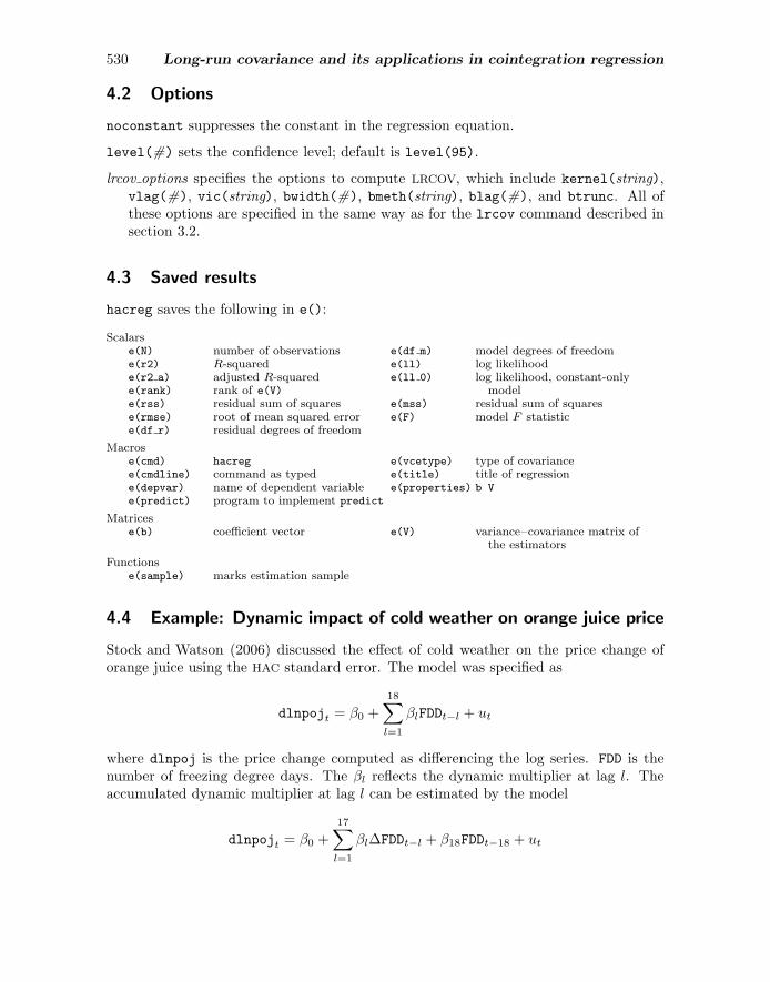
5.4 Saved results

cointreg saves the following in e():

Scalarse(N) number of observations e(r2) R-squarede(r2 a) adjusted R-squared e(rmse) standard errore(lrse) long-run standard error e(rss) residual sum of squarese(tss) total sum of squares e(eqtrend) trend term in equatione(xtrend) trend term in regressor e(bwidth) band widthe(vlag) lag in VAR prewhitening e(dlead) lead length in DOLSe(dlag) lag length in DOLS

Macrose(cmd) cointreg e(est) estimation methode(cmdline) command as typed e(vic) information criterion in VARe(kernel) kernel type e(bmeth) bandwidth selection methode(depvar) name of dependent variable e(properties) b Ve(dic) lag type in DOLS e(vcetype) variance type in DOLS

Matricese(b) coefficient vector e(V) variance–covariance matrix of

the estimators

Functionse(sample) marks estimation sample

5.5 Examples

Next we will illustrate the FMOLS, CCR, and DOLS cointegration estimation methodsusing several classical examples.

FMOLS example: The consumption function in the U.S.

We use the example in Hansen (1992) to illustrate FMOLS estimation. The data containseasonally adjusted aggregate quarterly U.S. consumption (tc) and total disposableincome (di) in real per capita units, for the period 1953:2–1984:4. The data can bedownloaded from Hansen’s homepage.3

A constant and a time trend are included in the equation:

tct = β0 + β1t+ β2dit + ut

We adopt the quadratic spectral kernel and the Andrews automatic bandwidth se-lection method. The following commands estimate the above equation. To replicate theresults of Hansen (1992), the nodivn option must be specified.

3. http://www.ssc.wisc.edu/˜bhansen/


. use campbell, clear

. cointreg tc di, est(fmols) vlag(1) kernel(qs) bmeth(andrews) eqtrend(1) nodivn

Cointegration regression (FMOLS):

VAR lag(user) = 1 Number of obs = 126Kernel = qs R2 = .9947833Bandwidth(andrews) = 0.8877 Adjusted R2 = .9946985

S.e. = 51.41235Long run S.e. = 108.0174

tc Coef. Std. Err. z P>|z| [95% Conf. Interval]

di .9818777 .0882267 11.13 0.000 .8089565 1.154799linear -1.022808 1.829954 -0.56 0.576 -4.609453 2.563836_cons -112.1549 194.2193 -0.58 0.564 -492.8177 268.508

The linear in the output table denotes the linear trend in the regression equation.

CCR example: The consumption of nondurable goods

We use the example of Ogaki (1993). The model is specified as

ndurt = β0 + β1pricet + β2durt + ut

where ndurt is real consumption of nondurable goods per capital, durt is real consump-tion of durable goods per capital, and pricet is the relative price index of nondurableand durable goods. The data can be downloaded from Ogaki’s homepage.4

We use the quadratic spectral kernel and the Andrews automatic bandwidth selectionmethod. The three-stage CCR regression is estimated by the following commands:

. use ccr

. cointreg ndur price dur, est(ccr) vlag(1) kernel(qs) bmeth(andrews) stage(3)

Cointegration regression (CCR):

VAR lag(user) = 1 Number of obs = 168Kernel = qs R2 = .4551902Bandwidth(andrews) = 0.5839 Adjusted R2 = .4485864

S.e. = .1514857Long run S.e. = .0866897

ndur Coef. Std. Err. z P>|z| [95% Conf. Interval]

price .5682032 .1385131 4.10 0.000 .2967225 .839684dur .5092836 .0448642 11.35 0.000 .4213515 .5972158

_cons 4.590851 .326225 14.07 0.000 3.951462 5.23024

4. http://www.econ.ohio-state.edu/ogaki/


DOLS example: The demand for money in the United States

The money demand equation typically estimated in the literature is specified as

mt − pt = µ+ θyyt + θrrt + ut

where mt is the log of money stock in period t, pt is the log of price level, yt is logincome, rt is nominal interest rate, and ut is the error term. θy is income elasticity andθr is the interest semielasticity of money demand. Hayashi (2000) cited this example inhis textbook; the data are downloadable from his homepage.5

All the variables are I(1), and we skip the unit-root testing and directly fit the modelusing the DOLS method. We fit the model using the full sample and two subsampleswith two leads and two lags, in accordance with Stock and Watson (1993). The LRCOV

is computed using prewhitening with the AR(2) model. The following commands repeatthe results of table 10.2 in Hayashi (2000), which consist of static ordinary least-squaresand DOLS estimations.

. use sw93(Source: Stock and Watson(1993))

. qui cointreg mp y r if tin(1903, 1987), est(dols) dlag(-1) kernel(none)

. qui estimates store SOLS

. qui cointreg mp y r, est(dols) dlead(2) dlag(2) vlag(2) kernel(none)

. qui estimates store DOLS

. estimates table SOLS DOLS, b(%6.3f) se(%6.3f) drop(_cons) style(oneline)

Variable SOLS DOLS

y 0.943 0.9700.022 0.046

r -0.082 -0.1010.006 0.013

legend: b/se

For the Chow break-point test at year 1946, Hayashi (2000) fit the model

mt − pt = µ+ γyyt + γrrt + δ0Dt + δyytDt + δrrtDt + ut

where Dt is a dummy variable whose value is 1 if t ≥ 1946 and 0 otherwise. We usefactor variables in Stata to fit the model, and we use the standard test command todo the Chow test:

5. http://fhayashi.fc2web.com/datasets.htm


. generate dum=year>=1946

. qui cointreg mp y r i.dum i.dum#c.(y r), est(dols) dlead(2) dlag(2) vlag(2)> kernel(none)

. test 1.dum 1.dum#c.y 1.dum#c.r

( 1) 1.dum = 0( 2) 1.dum#c.y = 0( 3) 1.dum#c.r = 0

chi2( 3) = 19.12Prob > chi2 = 0.0003

Note that only the differenced variables of (yt, rt) enter into the DOLS equation, sowe should have specified the dvar(y r) option. Hayashi (2000) listed the results intable 10.4.

6 Conclusion and extension

In time-series econometrics, estimating the long-run variance matrix of a random vec-tor process is essential for empirical research on estimation (for example, GMM andcointegration regression) and testing (for example, HAC standard error, unit root, andcointegration testing) problems. We propose the lrcov command to compute LRCOV;lrcov includes many kernel functions and allows the user to prewhiten the data. Basedon lrcov, we provide two other commands, hacreg and cointreg. hacreg estimatesHAC standard errors. Compared with the official Stata newey command, hacreg is moreflexible in that it contains more kernel functions, automatically determines the lag order,and prewhitens the data. cointreg estimates three cointegration regressions: FMOLS,DOLS, and CCR, all of which need to compute the LRCOV. We use several examples toillustrate these commands.

Many extensions can be made based on our work. More kernels and more bandwidthselection methods can be allowed in LRCOV estimation. Some examples may includefurther extensions on the lrcov command. Phillips, Sun, and Jin (2007) pursued theapproach of Kiefer and Vogelsang (2002a,b) and proposed a class of steep origin kernels,which are constructed by exponentiating a mother kernel and can be used withouttruncation. The steep origin kernels are asymptotically mean squared error equivalent,so choice of mother kernel does not matter asymptotically. Jin, Phillips, and Sun (2006)used steep origin kernels in cointegrated systems, and simulations indicated that robusttests have improved size and power properties.

Hirukawa (2010) suggested a two-stage plug-in bandwidth selection approach thatestimates an unknown quantity in the optimal bandwidth for the HAC estimator (callednormalized curvature) using a general class of kernels, and derives the optimal band-width that minimizes the asymptotic mean squared error of the estimator of normalizedcurvature. It is shown that the optimal bandwidth for the kernel-smoothed normalizedcurvature estimator should diverge at a slower rate than that of the HAC estimatorusing the same kernel. Hirukawa (2011) revealed that the new bandwidth choice rulecontributes bias reduction in the estimators for cointegration regression models.


LRCOV for more stochastic processes may be another important aspect for exten-sion. Phillips and Kim (2007) derived an asymptotic expansion for the autocovariancematrix of a vector of stationary long-memory processes and applied the theory to de-liver formulas for the LRCOV matrices of multivariate time series with long memory.Abadir, Distaso, and Giraitis (2009) extended the usual Bartlett-kernel HAC estimatorto deal with long memory and antipersistence, and derived asymptotic expansions forthis estimator and the memory and autocorrelation consistent estimator.

7 Acknowledgments

We would like to thank H. Joseph Newton (the editor) for providing advice and en-couragement. Constructive comments and insightful suggestions from an anonymousreferee, Jian Yang, and Liuling Li substantially helped the revision of this article. Wealso thank B. E. Hansen, M. Ogaki, and F. Hayashi. The data in our examples are di-rectly downloaded from their respective websites. Qunyong Wang acknowledges Project“Signal Extraction Theory and Applications of Robust Seasonal Adjustment” (GrantNo. 71101075) supported by NSFC and the Center for Experimental Education of Eco-nomics at Nankai University.

8 ReferencesAbadir, K. M., W. Distaso, and L. Giraitis. 2009. Two estimators of the long-run

variance: Beyond short memory. Journal of Econometrics 150: 56–70.

Andrews, D. W. K. 1991. Heteroskedasticity and autocorrelation consistent covariancematrix estimation. Econometrica 59: 817–858.

Andrews, D. W. K., and J. C. Monahan. 1992. An improved heteroskedasticity andautocorrelation consistent covariance matrix estimator. Econometrica 60: 953–966.

Brillinger, D. R. 1980. Time Series: Data Analysis and Theory. New York: Holt,Rinehart and Winston.

Choi, I., J. Y. Park, and B. Yu. 1997. Canonical cointegrating regression and testingfor cointegration in the presence of I(1) and I(2) variables. Econometric Theory 13:850–876.

Christou, C., and N. Pittis. 2002. A nonparametric prewhitened covariance estimator.Econometric Theory 18: 948–961.

den Haan, W. J., and A. Levin. 1996. Inferences from parametric and non-parametriccovariance matrix estimation procedures. NBER Technical Working Paper No. 195.http://www.nber.org/papers/t0195.html.

———. 1997. A practitioner’s guide to robust covariance matrix estimation. In Hand-

book of Statistics 15: Robust Inference, ed. G. S. Maddala and C. R. Rao, 291–341.Amsterdam: North-Holland.


———. 2000. Robust covariance matrix estimation with data-dependent VAR prewhiten-ing order. NBER Technical Working Paper No. 255.http://www.nber.org/papers/t0255.

Hall, A. R. 2005. Generalized Method of Moments. Oxford: Oxford University Press.

Hansen, B. E. 1992. Tests for parameter instability in regressions with I(1) processes.Journal of Business and Economic Statistics 10: 321–335.

Hayashi, F. 2000. Econometrics. Princeton, NJ: Princeton University Press.

Hirukawa, M. 2010. A two-stage plug-in bandwidth selection and its implementationfor covariance estimation. Econometric Theory 26: 710–743.

———. 2011. How useful is yet another data-driven bandwidth in long-run varianceestimation? A simulation study on cointegrating regressions. Economics Letters 111:170–172.

Jin, S., P. C. B. Phillips, and Y. Sun. 2006. A new approach to robust inference incointegration. Economics Letters 91: 300–306.

Kiefer, N. M., and T. J. Vogelsang. 2002a. Heteroskedasticity-autocorrelation robusttesting using bandwidth equal to sample size. Econometric Theory 18: 1350–1366.

———. 2002b. Heteroskedasticity-autocorrelation robust standard errors using theBartlett kernel without truncation. Econometrica 70: 2093–2095.

Lee, C. C., and P. C. B. Phillips. 1994. An ARMA prewhitened long-run varianceestimator. Working paper, Yale University.http://korora.econ.yale.edu/phillips/papers/prewhite.pdf.

Marmol, F., and C. Velasco. 2004. Consistent testing of cointegrating relationships.Econometrica 72: 1809–1844.

Newey, W. K., and K. D. West. 1987. A simple, positive semi-definite, heteroskedasticityand autocorrelation consistent covariance matrix. Econometrica 55: 703–708.

———. 1994. Automatic lag selection in covariance matrix estimation. Review of

Economic Studies 61: 631–653.

Ogaki, M. 1993. CCR: A user guide. RCER Working Papers 349, University of Rochester,Center for Economic Research. http://ideas.repec.org/p/roc/rocher/349.html.

Park, J. Y. 1992. Canonical cointegrating regressions. Econometrica 60: 119–143.

Park, J. Y., and M. Ogaki. 1991. Inference in cointegrated models using VAR prewhiten-ing to estimate shortrun dynamics. RCER Working Papers 281, University ofRochester, Center for Economic Research.http://ideas.repec.org/p/roc/rocher/281.html.


Pedroni, P. 2004. Panel cointegration: Asymptotic and finite sample properties of pooledtime series tests with an applicaton to the PPP hypothesis. Econometric Theory 20:597–625.

Phillips, P. C. B., and B. E. Hansen. 1990. Statistical inference in instrumental variablesregression with I(1) processes. Review of Economics Studies 57: 99–125.

Phillips, P. C. B., and C. S. Kim. 2007. Long-run covariance matrices for fractionallyintegrated processes. Econometric Theory 23: 1233–1247.

Phillips, P. C. B., and P. Perron. 1988. Testing for a unit root in time series regression.Biometrika 75: 335–346.

Phillips, P. C. B., Y. Sun, and S. Jin. 2007. Long run variance estimation using steeporigin kernels without truncation. Journal of Statistical Planning and Inference 137:985–1023.

Priestley, M. B. 1981. Spectral Analysis and Time Series. San Diego: Academic Press.

QMS. 2010. EViews 7.1 Supplement. Irvine, CA: Quantitative Micro Software.

Quintos, C. E. 1998. Fully modified vector autoregressive inference in partially nonsta-tionary models. Journal of the American Statistical Association 93: 783–795.

Saikkonen, P. 1992. Estimation and testing of cointegrated systems by an autoregressiveapproximation. Econometric Theory 8: 1–27.

StataCorp. 2009. Stata 11 Base Reference Manual. College Station, TX: Stata Press.

Stock, J. H., and M. Watson. 1993. A simple estimator of cointegrating vectors in higherorder integrated systems. Econometrica 61: 783–820.

Stock, J. H., and M. W. Watson. 2006. Introduction to Econometrics. 2nd ed. NewJersey: Prentice Hall.

Sul, D., P. C. B. Phillips, and C. Y. Choi. 2005. Prewhitening bias in HAC estimation.Oxford Bulletin of Economics and Statistics 67: 517–546.

White, H., and I. Domowitz. 1984. Nonlinear regression with dependent observations.Econometrica 52: 143–161.

Xiao, Z., and L. Oliver. 2002. A nonparametric prewhitened covariance estimator.Journal of Time Series Analysis 23: 215–250.

About the authors

Qunyong Wang earned his PhD from Nankai University. Now he works at the Institute ofStatistics and Econometrics at Nankai University. The article was written as part of hisinvolvement with the Stata research program in China.

Na Wu received her PhD from Nankai University. Now she works at the School of Economicsat Tianjin University of Finance and Economics. Her expertise lies in international economicsand the financial market.

Documents

The Stata Journal - AgEcon Searchageconsearch.umn.edu/bitstream/229441/2/sjart_st0272.pdf · The purpose of the Stata Journal is to promote free communication among Stata users. The