Embed Size (px)
Citation preview
Preprint 1
The Stability of Steady-State Hot-Spot Patterns for a
Reaction-Diffusion Model of Urban Crime
T. KOLOKOLNIKOV, M. J. WARD, and J. WEI
Theodore Kolokolnikov; Department of Mathematics, Dalhousie University, Halifax, Nova Scotia, B3H 3J5, Canada,
Michael Ward; Department of Mathematics, University of British Columbia, Vancouver, British Columbia, V6T 1Z2, Canada,
Juncheng Wei, Department of Mathematics, Chinese University of Hong Kong, Shatin, New Territories, Hong Kong.
(January 3rd, 2012)
The existence and stability of localized patterns of criminal activity are studied for the reaction-diffusion model of urban
crime that was introduced by Short et. al. [Math. Models. Meth. Appl. Sci., 18, Suppl. (2008), pp. 1249–1267]. Such
patterns, characterized by the concentration of criminal activity in localized spatial regions, are referred to as hot-spot
patterns and they occur in a parameter regime far from the Turing point associated with the bifurcation of spatially
uniform solutions. Singular perturbation techniques are used to construct steady-state hot-spot patterns in one and two-
dimensional spatial domains, and new types of nonlocal eigenvalue problems are derived that determine the stability
of these hot-spot patterns to O(1) time-scale instabilities. From an analysis of these nonlocal eigenvalue problems, a
critical threshold Kc is determined such that a pattern consisting of K hot-spots is unstable to a competition instability
if K > Kc. This instability, due to a positive real eigenvalue, triggers the collapse of some of the hot-spots in the
pattern. Furthermore, in contrast to the well-known stability results for spike patterns of the Gierer-Meinhardt reaction-
diffusion model, it is shown for the crime model that there is only a relatively narrow parameter range where oscillatory
instabilities in the hot-spot amplitudes occur. Such an instability, due to a Hopf bifurcation, is studied explicitly for a
single hot-spot in the shadow system limit, for which the diffusivity of criminals is asymptotically large. Finally, the
parameter regime where localized hot-spots occur is compared with the parameter regime, studied in previous works,
where Turing instabilities from a spatially uniform steady-state occur.
Key words: singular perturbations, hot-spots, reaction-diffusion, crime, nonlocal eigenvalue problem, Hopf Bifurca-tion.
1 Introduction
Recently, Short et. al. [29, 30, 31] introduced an agent-based model of urban crime that takes into account repeat or
near-repeat victimization. In dimensionless form, the continuum limit of this agent-based model is the two-component
reaction-diffusion PDE system
At = ε2∆A−A+ PA+ α , x ∈ Ω ; ∂nA = 0 , x ∈ ∂Ω , (1.1 a)
τPt = D∇ ·(
∇P − 2P
A∇A)
− PA+ γ − α , x ∈ Ω ; ∂nP = 0 , x ∈ ∂Ω , (1.1 b)
where the positive constants ε2, D, α, γ and τ , are all assumed to be spatially independent. In this model, P (x, t)
represents the density of the criminals, A(x, t) represents the “attractiveness” of the environment to burglary or
other criminal activity, and the chemotactic drift term −2D∇ ·(
P ∇AA
)
represents the tendency of criminals to move
towards sites with a higher attractiveness. In addition, α is the baseline attractiveness, while (γ − α)/τ represents
the constant rate of re-introduction of criminals after a burglary. For further details on the model see [29].
In [29], the reaction-diffusion system (1.1) with chemotactic drift term was derived from a continuum limit of
a lattice-based model. It was then analyzed using linear stability theory to determine a parameter range for the

2 T. Kolokolnikov, M. J. Ward, J. Wei
1.952
2.05 t=0.0
0
5 t=13.8
05
10 t=25.0
05
10 t=30.8
05
10 t=6032.3
01020 t=180246.0
01020 t=181178.0
0 0.5 10
1020 t=250000.0
1.952
2.05 t=0.0
1.52
2.5 t=8.7
05
10 t=23.1
05
10 t=35.9
05
10 t=42.9
05
10 t=729.4
0 0.5 105
10 t=250000.0
−1012 t=0.0 t=0.6
−1012 t=10.0 t=31.5
−1012 t=33.4 t=38.2
−1 0 1 2
−1012 t=48.6
−1 0 1 2
t=9000.0
(a) (b) (c)
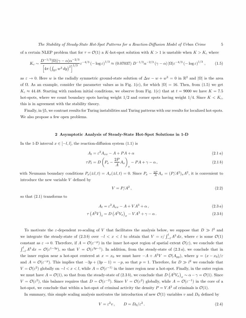
Figure 1. Numerical solution of (1.1) at different times, for initial data close to a spatially homogeneous steady-state. Plotsof A(x, t) are shown at the values of t indicated. (a) One dimensional domain with parameter values α = 1, γ = 2, ε = 0.02,τ = 1, D = 1. Initial conditions are P (x, 0) = 1 − α/γ and A(x, 0) = γ(1 − 0.01 cos(6πx)). Turing instability leads to aformation of three hot-spots; one is annihilated almost immediately due to a fast-time instability, while the second hot-spotis annihilated after a long time. (b) D = 0.5 with all other parameters as in (a). Two hot-spots remain stable. (c) Numericalsolution of (1.1) in a two-dimensional square of width 4. Parameters are α = 1, γ = 2, ε = 0.08, τ = 1, D = 1. Initial conditionsare P (x, 0) = 1− α/γ and A(x, 0) = γ(1 + rand ∗ 0.001) where rand generates a random number between 0 and 1.
existence of a Turing instability of the spatially uniform steady-state. A weakly nonlinear theory, based on a multi-
scale expansion valid near the Turing bifurcation point, was developed in [30, 31] for (1.1) for both one and two-
dimensional domains. This theoretical framework is very useful to explore the origins of various patterns that are
observed in full numerical solutions of the model. However, the major drawback of a weakly nonlinear theory is
that the parameters must be tuned near the bifurcation point of the Turing instability. When the parameters values
are at an O(1) distance from the bifurcation point, an instability of the spatially homogeneous steady-state often
leads to patterns consisting of localized structures. Such localized patterns for the crime model (1.1), consisting of
the concentration of criminal activity in localized spatial regions, are referred to as either hot-spot or spike-type
patterns. A localized hot-spot solution, not amenable to an analytical description by a weakly nonlinear analysis,
was observed in the full numerical solutions of [30].
As an illustration of localization behavior, in Fig. 1(a) we plot the numerical solution to (1.1) in the one-dimensional
domain Ω = [0, 1] with parameter values α = 1, γ = 2, ε = 0.02, τ = 1, and D = 1. The initial conditions, consisting
of a small mode-three perturbation of the spatially homogeneous steady-state Ae = γ and Pe = (γ − α)/γ are first
amplified due to linear instability. Shortly thereafter, nonlinear effects become significant and the solution quickly
becomes localized leading to the formation of three hot-spots, as shown at t ≈ 14. Subsequently, one of the hot-spots
appears to be unstable and is quickly annihilated. The remaining two hot-spots drift towards each other over a long
The Stability of Steady-State Hot-Spot Patterns for a Reaction-Diffusion Model of Urban Crime 3
time, until finally around t ≈ 180, 000, another hot-spot is annihilated. The lone remaining hot-spot then drifts
towards the center of the domain where it then remains. Next, in Fig. 1(b) we re-run the simulation when D is
decreased to D = 0.5 with all other parameters the same as in Fig. 1(a). For this value of D, we observe that the
final state consists of two hot-spots. Similar complex dynamics of hot-spots in a two-dimensional domain are shown
in Fig. 1(c).
It is the goal of this paper to give a detailed study of the existence and stability of steady-state localized hot-spot
patterns for (1.1) in both one and two-dimensional domains in the singularly perturbed limit
ε2 ≪ D . (1.2)
The assumption that ε2 ≪ D implies that the length-scale associated with the change in the attractiveness of
potential burglary sites is much smaller than the length-scale over which criminals explore new territory to commit
crime. In this limit, a singular perturbation methodology will be used to construct steady-state hot-spot solutions
and to derive new nonlocal eigenvalue problems (NLEP’s) governing the stability of these solutions. From an analysis
of the spectrum of these NLEP’s, explicit stability thresholds in terms of D and τ for the initiation of O(1) time-scale
instabilities of these patterns are obtained. In a one-dimensional domain, an additional stability threshold on D for
the initiation of slow translational instabilities of the hot-spot pattern is derived. Among other results, we will be
able to explain both the fast and slow instabilities of the localized hot-spots patterns as observed in Fig. 1(a).
In related contexts, there is now a rather large literature on the stability of spike-type patterns in two-component
reaction-diffusion systems with no drift terms. The theory was first developed in a one-dimensional domain to analyze
the stability of steady-state spike patterns for the Gierer-Meinhardt model (cf. [10, 3, 35, 37, 38, 34, 43, 46]) and,
in a parallel development, the Gray-Scott model (cf. [4, 5, 15, 23, 24, 18, 1]). The stability theory for these two
models was extended to two-dimensional domains in [39, 41, 40, 44, 43, 2]. Related studies for the Schnakenburg
model are given in [11, 36, 42]. The dynamics of quasi-equilibrium spike patterns is studied for one-dimensional
domains in [9, 6, 7, 33, 22], and in a multi-dimensional context in [13, 14, 16, 2]. More recently, in [19] the stability
of spikes was analyzed for a reaction-diffusion model of species segregation with cross-diffusion. A common feature
in all of these studies, is that an analysis of the spectrum of various classes of NLEP’s is central for determining
the stability properties of localized patterns. A survey of NLEP theory is given in [46], and in, a broader context, a
survey of phenomena and results for far-from-equilibrium patterns is given in [25].
In contrast, for reaction-diffusion systems with chemotactic drift terms, such as the crime model (1.1), there are
only a few studies of the existence and stability of spike solutions. These previous studies have focused mainly on
variants of the well-known Keller-Segel model (cf. [8, 12, 28, 32]).
We now summarize and illustrate our main results. In §2.1 we construct a multi hot-spot steady state solution
to (1.1) on a one-dimensional interval of length S. We refer to a symmetric hot-spot steady-state solution as one
for which the hot-spots are equally spaced and, correspondingly, each hot-spot has the same amplitude. In §2.2asymmetric steady-state hot-spot solutions, characterized by unevenly spaced hot-spots, are shown to bifurcate from
the symmetric branch of hot-spot solutions at a critical value of D.
In §3 we study the stability of steady-state K-hot-spot solutions on an interval of length S when τ = O(1). A
singular perturbation approach is used to derive a NLEP that determines the stability of these hot-spot patterns to
O(1) time-scale instabilities. In contrast to the NLEP’s arising in the study of spike stability for the Gierer-Meinhardt
model (cf. [35]), this NLEP is explicitly solvable. In this way, a critical threshold Kc+ is determined such that a
4 T. Kolokolnikov, M. J. Ward, J. Wei
pattern consisting of K hot-spots with K > 1 is unstable to a competition instability if and only if K > Kc+. This
instability, which develops on an O(1) time scale as ε → 0, is due to a positive real eigenvalue, and it triggers the
collapse of some of the hot-spots in the pattern. This critical threshold Kc+ > 0 is the unique root of (see Principal
Result 3.2 below)
K (1 + cos (π/K))1/4 =
(
S
2
)(
2
D
)1/4(γ − α)3/4√
πεα. (1.3)
In addition, from the location of the bifurcation point associated with the birth of an asymmetric hot-spot equilibrium,
a further threshold Kc− is derived that predicts that a K-hot-spot steady-state with K > 1 is stable with respect to
slow translational instabilities of the hot-spot locations if and only if K < Kc−. This threshold is given explicitly by
(see (3.20) below)
Kc− =
(
S
2
)
D−1/4 (γ − α)3/4√πεα
. (1.4)
Since Kc− < Kc+, the stability properties of a K-hot-spot steady-state solution with K > 1 and τ = O(1) are as
follows: stability when K < Kc−; stability with respect to O(1) time-scale instabilities but unstable with respect to
slow translation instabilities when Kc− < K < Kc+; a fast O(1) time-scale instability dominates when K > Kc+.
As an illustration of these results consider again Fig. 1(a). From the parameter values in the figure caption we
compute from (1.3) and (1.4) that Kc+ ≈ 2.273 and Kc− ≈ 1.995. Therefore, we predict that the three hot-spots
that form at t = 13.8 are unstable on an O(1) time-scale. This is confirmed by the numerical results shown at times
t = 25 and t = 30.8 in Fig. 1(a). We then predict from the threshold Kc− that the two-hot-spot solution will become
unstable on a very long time interval. This is also confirmed by the full numerical solutions shown in Fig. 1(a). In
contrast, if we decrease D to D = 0.5 as in Fig. 1(b) then we calculate from (1.3) and (1.4) that Kc+ ≈ 2.612 and
Kc− ≈ 2.372. Our prediction is that the three hot-spot solution that emerges from initial data will be unstable on
an O(1) time-scale, but that a two-hot-spot steady-state will be stable. These predictions are again corroborated by
the full numerical results.
In §4 we examine oscillatory instabilities of the amplitudes of the hot-spots in terms of the bifurcation parameter τ
in (1.1). From an analysis of a new NLEP with two separate nonlocal terms, we show that an oscillatory instability of
the hot-spot amplitudes as a result of a Hopf bifurcation is not possible on the regime τ ≤ O(ε−1). This non-existence
result for a Hopf bifurcation is in contrast to the results obtained in [35] for the Gierer-Meinhardt model showing
the existence of oscillatory instabilities of the spike amplitudes in a rather wide parameter regime. However, for the
asymptotically larger range of τ with τ = O(ε−2), in §4.1 we study oscillatory instabilities of a single hot-spot in
the simplified system corresponding to letting D → ∞ in (1.1). In this shadow system limit, we show for a domain
of length one that low frequency oscillations of the spot amplitude due to a Hopf bifurcation will occur when τ > τc
where
τc ∼ 0.039759(γ − α)3α−2ε−2 .
In §5 we extend our results to two dimensional domains. We first construct a quasi-equilibrium multi hot-spot
pattern, and then derive an NLEP governing O(1) time-scale instabilities of the spot pattern. As in the analyses of
[39, 40, 41, 42, 43, 44] for the Gierer-Meinhardt and Gray-Scott models, our existence and stability theory for
localized hot-spot solutions is accurate only to leading-order in powers of −1/ log ε. In §5.1, we show from an analysis
The Stability of Steady-State Hot-Spot Patterns for a Reaction-Diffusion Model of Urban Crime 5
of a certain NLEP problem that for τ = O(1) a K-hot-spot solution with K > 1 is unstable when K > Kc where
Kc ∼D−1/3|Ω|(γ − α)α−2/3
[
4π(∫
R2 w3 dy)2]1/3
ε−4/3 (− log ε)1/3 ≈ (0.07037) D−1/3α−2/3 (γ − α) |Ω|ε−4/3 (− log ε)
1/3, (1.5)
as ε → 0. Here w is the radially symmetric ground-state solution of ∆w − w + w3 = 0 in R2 and |Ω| is the area
of Ω. As an example, consider the parameter values as in Fig. 1(c), for which |Ω| = 16. Then, from (1.5) we get
Kc ≈ 44.48. Starting with random initial conditions, we observe from Fig. 1(c) that at t = 9000 we have K = 7.5
hot-spots, where we count boundary spots having weight 1/2 and corner spots having weight 1/4. Since K < Kc,
this is in agreement with the stability theory.
Finally, in §5, we contrast results for Turing instabilities and Turing patterns with our results for localized hot-spots.
We also propose a few open problems.
2 Asymptotic Analysis of Steady-State Hot-Spot Solutions in 1-D
In the 1-D interval x ∈ [−l, l], the reaction-diffusion system (1.1) is
At = ε2Axx −A+ PA+ α (2.1 a)
τPt = D
(
Px − 2P
AAx
)
x
− PA+ γ − α , (2.1 b)
with Neumann boundary conditions Px(±l, t) = Ax(±l, t) = 0. Since Px − 2PA Ax = (P/A2)xA
2, it is convenient to
introduce the new variable V defined by
V = P/A2 , (2.2)
so that (2.1) transforms to
At = ε2Axx −A+ V A3 + α , (2.3 a)
τ(
A2V)
t= D
(
A2Vx)
x− V A3 + γ − α . (2.3 b)
To motivate the ε-dependent re-scaling of V that facilitates the analysis below, we suppose that D ≫ l2 and
we integrate the steady-state of (2.3 b) over −l < x < l to obtain that V = c/∫ l
−lA3 dx, where c is some O(1)
constant as ε → 0. Therefore, if A = O(ε−p) in the inner hot-spot region of spatial extent O(ε), we conclude that∫ l
−lA3 dx = O(ε1−3p), so that V = O(ε3p−1). In addition, from the steady-state of (2.3 a), we conclude that in
the inner region near a hot-spot centered at x = x0 we must have −A + A3V = O(Ayy), where y = (x− x0)/ε
and A = O(ε−p). This implies that −3p + (3p − 1) = −p, so that p = 1. Therefore, for D ≫ l2 we conclude that
V = O(ε2) globally on −l < x < l, while A = O(ε−1) in the inner region near a hot-spot. Finally, in the outer region
we must have A = O(1), so that from the steady-state of (2.3 b), we conclude that D(
A2Vx)
x∼ α− γ = O(1). Since
V = O(ε2), this balance requires that D = O(ε−2). Since V = O(ε2) globally, while A = O(ε−1) in the core of a
hot-spot, we conclude that within a hot-spot of criminal activity the density P = V A2 of criminals is O(1).
In summary, this simple scaling analysis motivates the introduction of new O(1) variables v and D0 defined by
V = ε2v , D = D0/ε2 . (2.4)
6 T. Kolokolnikov, M. J. Ward, J. Wei
In terms of (2.4), (2.3) transforms to
At = ε2Axx −A+ ε2vA3 + α , −l < x < l ; Ax(±l, t) = 0 , (2.5 a)
τε2(
A2v)
t= D0
(
A2vx)
x− ε2vA3 + γ − α , −l < x < l ; vx(±l, t) = 0 . (2.5 b)
2.1 A Single Steady-State Hot-Spot Solution
We will now construct a steady-state hot-spot solution on the interval −l < x < l with a peak at the origin. In order to
construct a K-hot-spot pattern on a domain of length S, with evenly spaced spots, we need only set l = S/(2K) and
perform a periodic extension of the results obtained below on the basic interval −l < x < l. As such, the fundamental
problem considered below is to asymptotically construct a one-hot-spot steady-state solution on −l < x < l.
In the inner region, near the center of the hot-spot at x = 0, we expand A and v as
A =A0
ε+A1 + · · · , v = v0 + εv1 + · · · , y = x/ε . (2.6)
From (2.5 a) we obtain, in terms of y, that Aj(y) for j = 0, 1 satisfy
A′′
0 −A0 + v0A30 = 0 , −∞ < y <∞ , (2.7 a)
A′′
1 −A1 ++3A20A1v0 = −α− v1A
30 , −∞ < y <∞ . (2.7 b)
In contrast, from (2.5 b), we obtain that vj for j = 0, 1 satisfy
(
A20v
′
0
)′= 0 ,
(
A20v
′
1 + 2A0A′
1v′
0
)′= 0 , −∞ < y <∞ . (2.8)
In order to match to an outer solution, we require that v0 and v1 are bounded as |y| → ∞. In this way, we then
obtain that v0 and v1 must both be constants, independent of y.
We look for a solution to (2.7) for which the hot-spot has a maximum at y = 0. The homoclinic solution to (2.7 a)
with A′0(0) = 0 is written as
A0(y) = v−1/20 w(y) , (2.9)
where w is the unique solution to the ground-state problem
w′′ − w + w3 = 0 , −∞ < y <∞ ; w(0) > 0 , w′(0) = 0 ; w → 0 as |y| → ∞ , (2.10)
given explicitly by w =√2 sech y. Next, we decompose the solution A1 to (2.7 b) as
A1 = α− v1
2v3/20
w − 3αw1 ,
where w1(y) satisfies
L0w1 ≡ w′′
1 − w1 + 3w2w1 = w2 , −∞ < y <∞ , (2.11)
with w′1(0) = 0 and w1 → 0 as |y| → ∞.
A key property of the operator L0, which relies on the cubic exponent in (2.10), is the remarkable identity that
L0w2 = 3w2 . (2.12)
The proof of this identity is a straightforward manipulation of (2.10) and the operator L0 in (2.11). This property
The Stability of Steady-State Hot-Spot Patterns for a Reaction-Diffusion Model of Urban Crime 7
plays an important role in an explicit analysis of the spectral problem in §3. Here this identity is used to provide an
explicit solution to (2.11) in the form
w1 = w2/3 .
In this way, in the inner region the two-term expansion for A in terms of the unknown constants v0 and v1 is
A(y) ∼ ε−1A0(y) +A1(y) + · · · , A0(y) = ε−1v−1/20 w(y) , A1(y) = α
(
1− [w(y)]2)
− v1
2v3/20
w(y) . (2.13)
In the outer region, defined for ε≪ |x| ≤ l, we have that v = O(1) and that A = O(1). From (2.5), we obtain that
A = α+ o(1) , v = h0(x) + o(1) ,
where from (2.5 b), h0(x) satisfies
h0xx = ζ ≡ (α− γ)
D0α2< 0 , 0 < |x| ≤ l ; h0x(±l) = 0 ,
subject to the matching condition that h0 → v0 as x→ 0±. The solution to this problem gives the outer expansion
v ∼ h0(x) =ζ
2
[
(l − |x|)2 − l2]
+ v0 , 0 < |x| ≤ l . (2.14)
Next, we must calculate the constants v0 and v1 appearing in (2.13) and (2.14). We integrate (2.5 b) over −l < x < l
and use vx = 0 at x = ±l to get
ε2∫ l
−l
vA3 dx = 2l(α− γ) .
Since A = O(ε−1) in the inner region, while A = O(1) in the outer region, the dominant contribution to the integral
in (2.1) arises from the inner region where x = O(ε). If we use the inner expansion A = ε−1A0 + A1 + o(1) from
(2.13), and change variables to y = ε−1x, we obtain from (2.1) that
v0
∫ ∞
−∞
A30 dy + ε
(
3v0
∫ ∞
−∞
A20A1 dy + v1
∫ ∞
−∞
A30
)
+O(ε2) = 2l(α− γ) . (2.15)
In (2.15), we emphasize that the first two terms on the left-hand side arise solely from the inner expansion, whereas
the O(ε2) term would be obtained from both the inner and outer expansions. By equating coefficients of ε in (2.15),
we obtain that
v0 = 2l(γ − α)/
∫ ∞
−∞
A30 dy , v1 = −3v0
∫ ∞
−∞
A20A1 dy/
∫ ∞
−∞
A30 dy ,
Then, upon using (2.13) for A0 and A1, together with w =√2 sech y,
∫∞
−∞w3 dy =
√2π, and
∫∞
−∞w4 dy = 16/3, we
readily derive from (2.1) that
v0 =π2
2l2 (α− γ)2, v1 = 6v
3/20 α
(∫∞
−∞
(
w2 − w4)
dy∫∞
−∞w3 dy
)
= −4√2
πv3/20 α = − 2απ2
l3(γ − α)3. (2.16)
We summarize our result for a single steady-state hot-spot solution as follows:
Principal Result 2.1: Let ε → 0, and consider a one-hot-spot solution centered at the origin for (2.5) on the
interval |x| ≤ l. Then, in the inner region y = x/ε = O(1), we have
A(y) =w
ε√v0
+ α
(
1 +2√2
πw − w2
)
+ o(1) , v ∼ v0 + εv1 + · · · . (2.17)
In addition, in the inner region, the leading-order steady-state criminal density P from (2.1) is P ∼ w2. Here w =

8 T. Kolokolnikov, M. J. Ward, J. Wei
0
2
4
6
8
10
12
14
A
0.2 0.4 0.6 0.8 1x
4.2
4.4
4.6
4.8
5
5.2
5.4
v
0 0.2 0.4 0.6 0.8 1x
(a) (b)
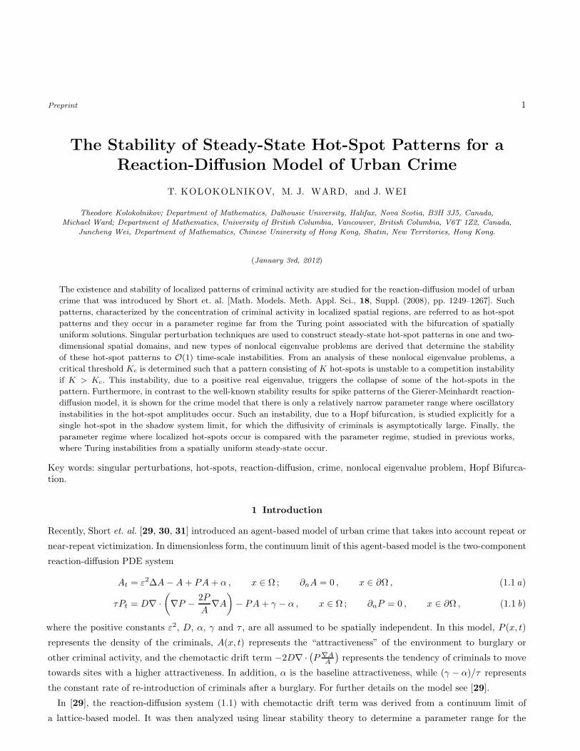
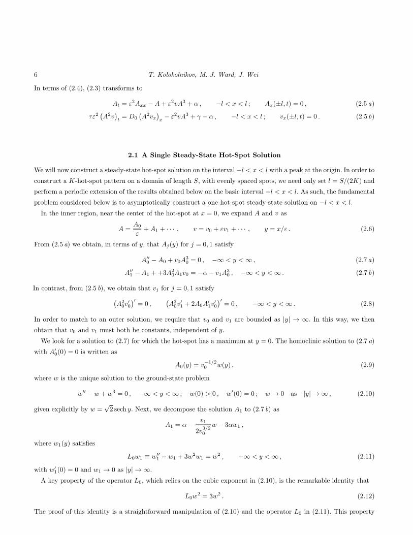
Figure 2. Steady-state solution in one spatial dimension. Parameter values are D0 = 1, ε = 0.05, α = 1, γ = 2, and x ∈ [0, 1].(a) The solid line is the steady state solution A(x) of (2.5) computed by solving the boundary value problem numerically.The dashed line corresponds to the first-order composite approximation given by (2.19) (b) The solid line is the steady statesolution for v(x). Note the “flat knee” region obtained from the full numerical solution in the inner region near the center ofthe hot-spot. The dashed line is the leading-order asymptotic result (2.18).
ε A(0) (num) A(0) (asy1) A(0) (asy2) v(0) (num) v(0) (asy1) v(0) (asy2)
0.1 6.281 6.366 6.003 3.5844 4.935 2.9610.05 12.805 12.732 12.369 4.1474 4.935 3.9480.025 25.628 25.465 25.101 4.4993 4.935 4.4410.0125 51.145 50.930 50.566 4.7039 4.935 4.688
Table 1. Comparison of numerical and asymptotic results for the amplitude Amax ≡ A(0) and for v(0) of a one-hot-
spot solution on [−1, 1] with D0 = 1, γ = 1, and α = 2. The 1-term and 2-term asymptotic results for Amax and v(0)
are obtained from (2.17).
w(y) =√2 sech y is the homoclinic of (2.10), while v0 and v1 are given in (2.16). In the outer region, O(ε) < |x| ≤ l,
then
A ∼ α+ o(1) ; v ∼ ζ
2
(
(l − |x|)2 − l2)
+ v0 + o(1) , ζ ≡ (α− γ)
D0α2< 0 . (2.18)
Note that to get a solution for A which is uniformly valid in both inner and outer region, we can combine the
formulas (2.17) and (2.18). The resulting first-order composite solution is given explicitly by
A ∼(
2l(γ − α)
πε− α
)
sech(x
ε
)
+ α . (2.19)
For a specific parameter set, a comparison of the full numerical steady-state solution of (2.5) with the composite
asymptotic solution (2.19) is shown in Fig. 2. A comparison of numerical and asymptotic values for A(0) and v(0) at
various ε is shown in Table 1. From this table we note that the two-term asymptotic expansion for v(0) agrees very
favorably with full numerical results.
The Stability of Steady-State Hot-Spot Patterns for a Reaction-Diffusion Model of Urban Crime 9
2.2 Asymmetric Steady-State K-Hot-Spot Solutions
In the limit ε→ 0, we now construct an asymmetric steady-stateK-hot-spot solution to (2.5) in the form of a sequence
of hot-spots of different heights. This construction will be used to characterize the stability of symmetric steady-state
K-hot-spot solutions with respect to the small eigenvalues λ = o(1) in the spectrum of the linearization. Since the
asymmetric solution is shown to bifurcate from the symmetric branch, the point of the bifurcation corresponds to a
zero eigenvalue crossing along the symmetric branch. To determine this bifurcation point, we compute v(l) for the
one-hot-spot steady-state solution to (2.5) on |x| ≤ l, where l > 0 is a parameter. This canonical problem is shown
to have two different solutions. A K-hot-spot asymmetric solution to (2.5) is then obtained by using translates of
these two local solutions in such a way to ensure that the resulting solution is C1 continuous. Since the details of
the construction of the asymmetric solution is very similar to that in [36] for the Schnakenburg model, we will only
give a brief outline of the analysis.
The key quantity of interest is the critical value Ds0K of D for which an asymmetric K-hot-spot solution branch
bifurcates off of the symmetric branch. To this end, we first calculate from (2.14) that
v(l) =(γ − α)
2α2√D0
B (l/q) , q ≡(
D0π2α2
(γ − α)3
)1/4
, (2.20 a)
where the function B(z) on 0 < z <∞ is defined by
B(z) ≡ z2 + 1/z2 . (2.20 b)
The function B(z) > 0 in (2.20 b) has a unique global minimum point at z = zc = 1, and it satisfies B′
(z) < 0 on
[0, zc) and B′(z) > 0 on (zc,∞). Therefore, given any z ∈ (0, zc), there exists a unique point z ∈ (zc,∞) such that
B(z) = B(z). This shows that given any l, with l/q < zc = 1, there exists a unique l, with l/q ≡ z > zc = 1, such
that v(l) = v(l).
We refer to solutions of length l and l as A-type and B-type hot-spots. Now consider the interval x ∈ [a, b] with
length S ≡ b − a. To construct a K-hot-spot steady-state solution to (2.5) on this interval with K1 ≥ 0 hot-spots
of type A and K2 = K −K1 ≥ 0 hot-spots of type B, arranged in any order across the interval, we must solve the
coupled system 2K1l + 2K2l = S and B(l/q) = B(l/q) for l 6= l. Such solution exists only if l/q < zc and l/q > zc
with zc = 1. The bifurcation point corresponds to the minimum point where l = l = q. With D = D0/ε2, this yields
that
l =
(
D0π2α2
(γ − α)3
)1/4
= ε1/2(
Dπ2α2
(γ − α)3
)1/4
. (2.21)
At this value of the parameters, a steady-stateK-hot-spot asymmetric solution branch bifurcates off of the symmetric
K-hot-spot branch. This critical value of D0 determines the small eigenvalue stability threshold in the linearization
of the symmetric K-hot-spot steady-state solution. For a symmetric configuration of K hot-spots on an interval of
length S we have 2Kl = S so that the critical value D0 = DS0K , as defined by (2.21), can be written as
DS0K =
(γ − α)3
π2α2
(
S
2K
)4
. (2.22)
A more detailed construction of the asymmetric solution branches parallels that done in [36] for the Schnakenburg
model and is left to the reader.
10 T. Kolokolnikov, M. J. Ward, J. Wei
3 The NLEP Stability of Steady-State 1-D Hot-Spot Patterns
We now study the stability of the K-hot-spot steady-state solution to (2.5) that was constructed in §2. The analysis
for the “large” O(1) eigenvalues in the spectrum of the linearization is done in several distinct steps.
Firstly, we let Ae, ve denote the one-hot-spot quasi-steady-state solution to (2.5) on the basic interval |x| ≤ l,
which was given in Principal Result 2.1. Upon introducing the perturbation
A = Ae + φeλt , v = ve + ψeλt , (3.1)
we obtain from the linearization of (2.5) that
ε2φxx − φ+ 3ε2veA2eφ+ ε3A3
eψ = λφ , (3.2 a)
D0
(
εA2eψx + 2Aevexφ
)
x− 3ε2A2
eveφ− ε3ψA3e = τλε2
(
εA2eψ + 2Aeveφ
)
. (3.2 b)
We consider (3.2 a) and (3.2 b) on |x| ≤ l subject to the Floquet-type boundary conditions
φ(l) = zφ(−l) , φ′(l) = zφ′(−l) , ψ(l) = zψ(−l) , ψ′(l) = zψ′(−l) , (3.2 c)
where z is a complex parameter.
For simplicity, in this section we will set τ = 0 in (3.2 b). The analysis of the possibility of Hopf bifurcations
induced by taking τ 6= 0 is studied in §4.After formulating the NLEP associated with solving (3.2) for arbitrary z, we then must determine z so that we
have the required NLEP problem for a K-hot-spot pattern on [−l, (2K−1)l] with periodic boundary conditions. This
is done by translating φ and ψ from the interval [−l, l] to the extended interval [−l, (2K− 1)l] in such a way that the
extended φ and ψ have continuous derivatives at x = l, 3l, . . . , (2K − 3)l. It follows that φ [(2K − 1)l] = zKφ(−l),and hence to obtain periodic boundary conditions on an interval of length 2Kl we require that zK = 1, so that
zj = e2πij/K , j = 0, . . . ,K − 1 . (3.3)
By using these values of zj in the NLEP problem associated with (3.2), we obtain the stability threshold of a K-
hot-spot solution on a domain of length 2Kl subject to periodic boundary conditions. The last step in the analysis
is then to extract the stability thresholds for the corresponding Neumann problem from the thresholds for the
periodic problem, and to choose l appropriately so that the Neumann problem is posed on [−1, 1]. This is done
below. This Floquet-based approach to determine the NLEP problem of a K-hot-spot steady-state solution for the
Neumann problem has been used previously for reaction-diffusion systems exhibiting mesa patterns [22], for the
Gierer-Meinhardt model [34], and for a cross-diffusion system [19].
We now implement the details of this calculation. The asymptotic analysis for ε → 0 of (3.2) proceeds as follows.
In the inner region with y = ε−1x, we use Ae = O(ε−1) and vex ≪ 1, to obtain from (3.2 b) that to leading order[
w2ψy
]
y= 0 in the inner region, where w is the homoclinic satisfying (2.10). To prevent exponential growth for ψ
as |y| → ∞, we must take ψ = ψ0 where ψ0 is a constant to be determined. Then, for (3.2 a) we look for a localized
inner eigenfunction in the form
φ ∼ Φ(y) , y = ε−1x .
Upon using the leading-order approximation Ae ∼ ε−1v−1/20 w in (3.2 a), we obtain to leading order that Φ(y) satisfies
L0Φ+1
v3/20
w3ψ0 = λΦ , −∞ < y <∞ ; L0Φ ≡ Φ′′ − Φ + 3w2Φ , (3.4)
The Stability of Steady-State Hot-Spot Patterns for a Reaction-Diffusion Model of Urban Crime 11
with Φ → 0 as |y| → ∞. Here v0 is given in (2.16).
In the outer region, away from the hot-spot centered at x = 0, we have Ae ∼ α and v = O(1), so that (3.2 a) yields
φ =ε3α3
λ+ 1ψ . (3.5)
Then, from (3.2 b), together with Ae ∼ α, we obtain the outer approximation D0
[
εα2ψx +O(ε3)]
x= O(ε3), which
yields the leading-order outer problem
ψxx = 0 , 0 < |x| ≤ l , (3.6)
subject to the Floquet-type boundary conditions (3.2 c). The matching condition for the inner and outer represen-
tations of ψ is that limx→0 ψ(x) = ψ0, where ψ0 is the unknown constant required in the spectral problem (3.4).
However, the problem for ψ is not yet complete, as it must be supplemented by appropriate jump conditions for ψx
across x = 0.
We now proceed to derive this jump condition. We first define an intermediate scale η satisfying ε ≪ η ≪ 1, and
we integrate (3.2 b) over |x| ≤ η to get
D0
(
εA2eψx + 2Aevexφ
)
|η−η =
∫ η
−η
(
3ε2A2eveφ+ ε3ψA3
e
)
dx . (3.7)
We use the limiting behavior as x→ 0± of the outer expansion to calculate the terms on the left hand-side of (3.7).
From Ae ∼ α, (2.14) to calculate vex(0±), and (3.5) to calculate φ(0±), we obtain that
D0
(
εA2eψx
)
|η−η ∼ D0εα2(
ψx(0+)− ψx(0
−))
= εD0α2 [ψx]0 , (3.8 a)
D0 (2Aevexφ) |η−η ∼ 2D0α[
φ(0+)vex(0+)− φ(0−)vex(0
−)]
= 4D0αφ(0+)vex(0
+) ∼ 4ε3α2
λ + 1ψ(0)(γ − α)l . (3.8 b)
Here we have defined [ψx]0 ≡ ψx(0+)− ψx(0
−).
Next, since η ≫ O(ε), we can estimate the integrals on the right-hand side of (3.7) by their contributions from the
inner approximation Ae ∼ ε−1v−1/20 w(y), ψ ∼ ψ0, φ ∼ Φ(y), and ve ∼ v0. In this way, we calculate
∫ η
−η
(
3ε2A2eveφ+ ε3ψA3
e
)
dx ∼ 3ε
∫ ∞
−∞
w2Φ dy +εψ0
v3/20
∫ ∞
−∞
w3 dy . (3.9)
Upon substituting (3.8) and (3.9) into (3.7), we obtain the following jump condition for ψx across x = 0:
D0α2 [ψx]0 = ψ0
(
v−3/20
∫ ∞
−∞
w3 dy − 4ε2α2
λ+ 1(γ − α)l
)
+ 3
∫ ∞
−∞
w2Φ dy . (3.10)
For the range λ > −1, we can neglect the negligible O(ε2) term in the jump condition (3.10). In this way, the
problem for the outer eigenfunction ψ(x) is to solve
ψxx = 0 , 0 < |x| ≤ l ; ψ(l) = zψ(−l) , ψ′(l) = zψ′(−l) , (3.11 a)
subject to the continuity condition ψ(0+) = ψ(0−) = ψ0 and the following jump condition across x = 0:
a0 [ψx]0 + a1ψ(0) = a2 ; a0 ≡ D0α2 , a1 = −v−3/2
0
∫ ∞
−∞
w3 dy , a2 = 3
∫ ∞
−∞
w2Φ dy . (3.11 b)
Upon calculating ψ(0) = ψ0 from this problem, the NLEP is then obtained from (3.4).
Upon solving (3.11) for ψ(x), and evaluating the result at x = 0 we get
v−3/20 ψ0 = −3
(∫∞
−∞w2Φ dy
∫∞
−∞w3 dy
)[
1−(
D0α2v
3/20
2l∫∞
−∞w3 dy
)
(z − 1)2
z
]−1
. (3.12)
12 T. Kolokolnikov, M. J. Ward, J. Wei
Next, we use (2.16) for v0 and∫∞
−∞w3 dy =
√2π to simplify v
−3/20 ψ0. In addition, we use (3.3) to calculate
(z − 1)2
z= −2 + 2Re(z) = −2 [1− cos (2πj/K)] , j = 0, . . . ,K − 1 . (3.13)
Upon substituting these results into (3.4), we obtain the following NLEP for a K-hot-spot steady-state on a domain
of length 2Kl subject to periodic boundary conditions:
L0Φ− χjw3
∫∞
−∞w2Φ dy
∫∞
−∞w3 dy
= λΦ , −∞ < y <∞ ; Φ → 0 , |y| → ∞ , (3.14 a)
χj ≡ 3
[
1 +D0α
2π2
4l4(γ − α)3(1− cos (2πj/K))
]−1
, j = 0, . . . ,K − 1 . (3.14 b)
The final step in the analysis is extract the NLEP for the Neumann problem from the NLEP (3.14) for the periodic
problem. More specifically, the stability thresholds for a K-hot-spot pattern with Neumann boundary conditions can
be obtained from the corresponding thresholds for a 2K-hot-spot pattern with periodic boundary conditions on a
domain of twice the length. To see this, suppose that φ is a Neumann eigenfunction on the interval [0, a]. Extend
it by an even reflection about the origin to the interval [−a, a]. Such an extension then satisfies periodic boundary
conditions on [−a, a]. Alternatively, if φ(x) is an eigenfunction with periodic boundary conditions at the edge of the
interval [−a, a], then define φ(x) = φ(x) +φ(−x). Then, φ is a eigenfunction for the Neumann boundary problem on
[0, a].
Therefore, to obtain the NLEP problem governing the stability of an steady-stateK-hot-spot pattern on an interval
of length S subject to Neumann boundary conditions, we simply replace cos(2πj/K) with cos(πj/K) in (3.14) and
then set l = S/(2K) in the NLEP of (3.14). In this way, we obtain the following main result:
Principal Result 3.1: Consider a K-hot-spot solution to (2.5) on an interval of length S subject to Neumann
boundary conditions. For ε → 0, and τ = O(1), the stability of this solution with respect to the “large” eigenvalues
λ = O(1) of the linearization is determined by the spectrum of the NLEP
L0Φ− χjw3
∫∞
−∞w2Φ dy
∫∞
−∞w3 dy
= λΦ , −∞ < y <∞ ; Φ → 0 , |y| → ∞ , (3.15 a)
χj = 3
[
1 +D0α
2π2K4
4(γ − α)3
(
2
S
)4
(1− cos (πj/K))
]−1
, j = 0, . . . ,K − 1 , (3.15 b)
where w(y) is the homoclinic solution satisfying w′′ − w + w3 = 0.
The stability threshold for D0 is characterized by the largest possible value of D0 for which the point spectrum
of (3.15) satisfies Re(λ) < 0 for each j = 0, . . . ,K − 1. In contrast to the typical NLEP problem associated with
spike patterns in the Gierer-Meinhardt, Gray-Scott, and Schnakeneburg reaction-diffusion models studied in [3], [4],
[5], [10], [15], [35], [36], and [43], the point spectrum for the non-self-adjoint problem (3.15) is real, and can be
determined analytically. This fact, as we now show, relies critically on the identity L0w2 = 3w2 from (2.12).
Lemma 3.2: Consider the NLEP problem
L0Φ− cw3
∫ ∞
−∞
w2Φ dy = λΦ , −∞ < y <∞ ; Φ → 0 , |y| → ∞ , (3.16)
for an arbitrary constant c corresponding to eigenfunctions for which∫∞
−∞w2Φ dy 6= 0. Consider the range Re(λ) >
The Stability of Steady-State Hot-Spot Patterns for a Reaction-Diffusion Model of Urban Crime 13
−1. Then, on this range there is only one element in the point spectrum, and it is given explicitly by
λ = 3− c
∫ ∞
−∞
w5 dy . (3.17)
To prove this we consider only the region Re(λ) > −1, where we can guarantee that |Φ| → 0 exponentially as
|y| → ∞. The continuous spectrum for (3.16) is λ < −1, with λ real. To establish (3.17) we use Green’s identity on
w2 and Φ, which is written as∫∞
−∞
(
w2L0Φ− ΦL0w2)
dy = 0. Since L0Φ = cw3∫∞
−∞w2Φ dy+ λΦ and L0w
2 = 3w2,
this identity reduces to∫ ∞
−∞
w2Φ dy
(
λ− 3 + c
∫ ∞
−∞
w5 dy
)
= 0 ,
from which the result (3.17) follows. We remark that for the corresponding local eigenvalue problem L0Φ = νΦ, it
was proved in Proposition 5.6 of [3] that the point spectrum consists only of ν0 = 3 and the translation mode ν1 = 0
(with odd eigenfunction), and that there are no other point spectra in −1 < ν < 0. When c = 0, we observe that
(3.17) agrees with ν0. As a further remark, the result (3.17), when extrapolated into the region λ < −1, suggests
that there is a critical value of c for which the discrete eigenvalue bifurcates out of the continuous spectrum into the
region λ > −1 on the real axis.
By applying Lemma 3.2 to the NLEP (3.15) we conclude that Re(λ) < 0 if and only if
χj < 3
(∫∞
−∞w3 dy
∫∞
−∞w5 dy
)
= 2 , j = 0, . . . ,K − 1 . (3.18)
In obtaining the last equality in (3.18) we calculated the integrals using w =√2 sech y. Since χ0 = 3 < χ1 < χ2 <
. . . χK−1, a one-hot-spot solution is stable for all D0, while the instability threshold for a multi hot-spot pattern is
set by χK−1. In this way, we obtain the following main stability result.
Principal Result 3.2: Consider a K-hot-spot solution to (2.5) on an interval of length S with K > 1 subject to
Neumann boundary conditions. For τ = 0, and in the limit ε → 0, this solution is stable on an O(1) time-scale
provided that D0 < DL0K
, where
DL0K ≡ 2(γ − α)3 (S/2)4
K4α2π2 [1 + cos (π/K)]. (3.19)
In terms of the original diffusivity D, given by D = ε−2D0, the stability threshold is DLK
= ε−2DL0K
when K > 1.
Alternatively, a one-hot-spot solution is stable for all D0 > 0, provided that D0 is independent of ε.
Although we have not calculated the stability threshold for the small eigenvalues for which λ→ 0 as ε→ 0 in the
spectrum of the linearization (3.2), we conjecture that this stability threshold is the same critical value DS0K of D0,
given in (2.22), for which an asymmetric K-hot-spot steady-state branch bifurcates off of the symmetric K-hot-spot
branch. This simple approach to calculate the small eigenvalue stability threshold, which avoids the lengthy matrix
manipulations of [10], has been validated for the Gierer-Meinhardt, Gray-Scott, and Schnakenburg reaction-diffusion
models in [37], [36], and [18]. Since DS0K < DL
0K for K ≥ 2, we conclude that a symmetric K-hot-spot steady-state
solution is stable with respect to both the large and the small eigenvalues only when D < DS0K.
We make two remarks. Firstly, for the case of a single hot-spot where K = 1 we expect that the stability threshold
for D0 will be exponentially large in 1/ε, and similar to that derived in [14] for the Gierer-Meinhardt model in the
near-shadow limit. Secondly, we remark that the possibility of stabilizing multiple hot-spots for (2.1) is in direct
contrast to the result obtained in the analysis of [32] of spike solutions for a Keller-Segel-type chemotaxis model with
14 T. Kolokolnikov, M. J. Ward, J. Wei
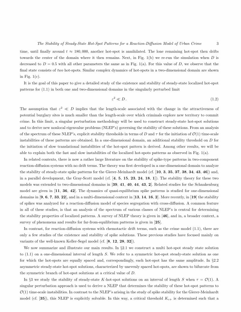
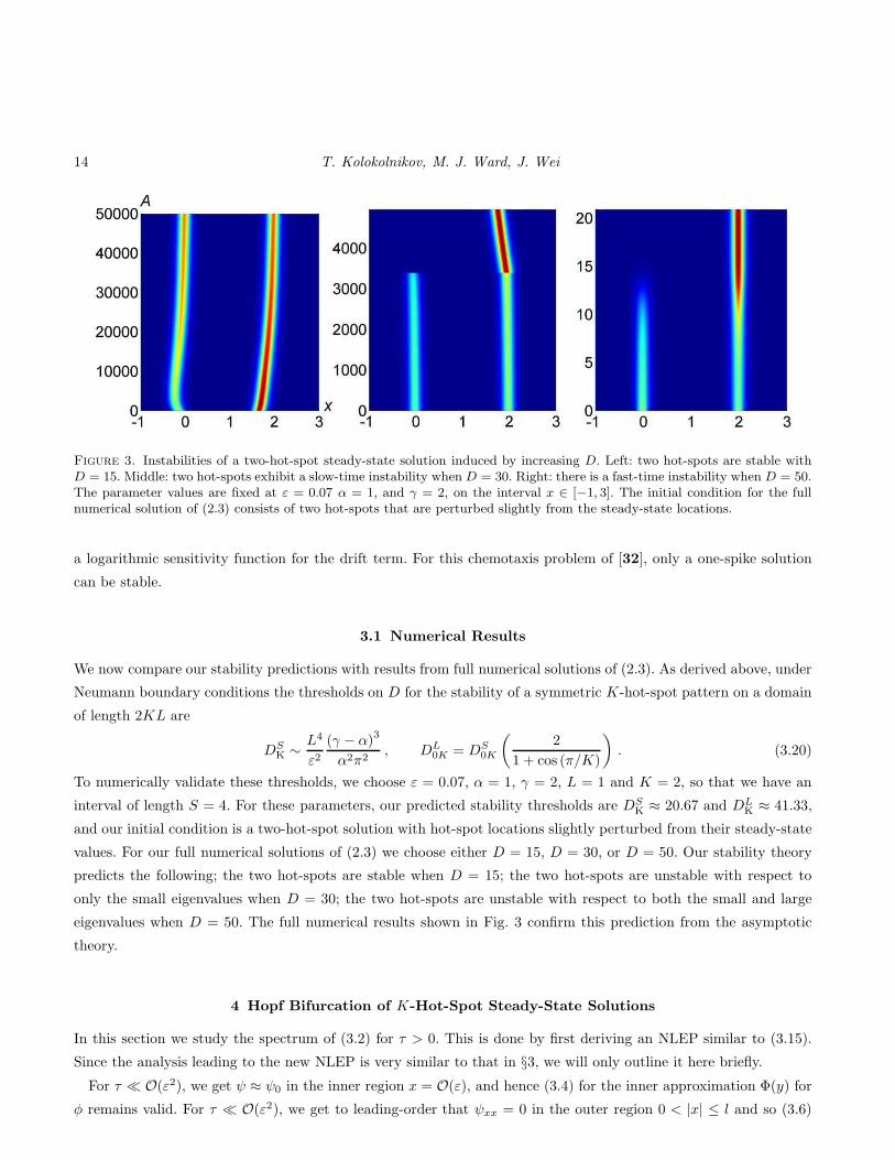
Figure 3. Instabilities of a two-hot-spot steady-state solution induced by increasing D. Left: two hot-spots are stable withD = 15. Middle: two hot-spots exhibit a slow-time instability when D = 30. Right: there is a fast-time instability when D = 50.The parameter values are fixed at ε = 0.07 α = 1, and γ = 2, on the interval x ∈ [−1, 3]. The initial condition for the fullnumerical solution of (2.3) consists of two hot-spots that are perturbed slightly from the steady-state locations.
a logarithmic sensitivity function for the drift term. For this chemotaxis problem of [32], only a one-spike solution
can be stable.
3.1 Numerical Results
We now compare our stability predictions with results from full numerical solutions of (2.3). As derived above, under
Neumann boundary conditions the thresholds on D for the stability of a symmetric K-hot-spot pattern on a domain
of length 2KL are
DSK ∼ L4
ε2(γ − α)3
α2π2, DL
0K = DS0K
(
2
1 + cos (π/K)
)
. (3.20)
To numerically validate these thresholds, we choose ε = 0.07, α = 1, γ = 2, L = 1 and K = 2, so that we have an
interval of length S = 4. For these parameters, our predicted stability thresholds are DSK ≈ 20.67 and DL
K ≈ 41.33,
and our initial condition is a two-hot-spot solution with hot-spot locations slightly perturbed from their steady-state
values. For our full numerical solutions of (2.3) we choose either D = 15, D = 30, or D = 50. Our stability theory
predicts the following; the two hot-spots are stable when D = 15; the two hot-spots are unstable with respect to
only the small eigenvalues when D = 30; the two hot-spots are unstable with respect to both the small and large
eigenvalues when D = 50. The full numerical results shown in Fig. 3 confirm this prediction from the asymptotic
theory.
4 Hopf Bifurcation of K-Hot-Spot Steady-State Solutions
In this section we study the spectrum of (3.2) for τ > 0. This is done by first deriving an NLEP similar to (3.15).
Since the analysis leading to the new NLEP is very similar to that in §3, we will only outline it here briefly.
For τ ≪ O(ε2), we get ψ ≈ ψ0 in the inner region x = O(ε), and hence (3.4) for the inner approximation Φ(y) for
φ remains valid. For τ ≪ O(ε2), we get to leading-order that ψxx = 0 in the outer region 0 < |x| ≤ l and so (3.6)
The Stability of Steady-State Hot-Spot Patterns for a Reaction-Diffusion Model of Urban Crime 15
still holds. However, for τ 6= 0, the jump conditions (3.7)–(3.9) must be modified. In place of (3.7), we get
D0
(
εA2eψx + 2Aevexφ
)
|η−η =
∫ η
−η
(
3ε2A2eveφ+ ε3ψA3
e
)
dx+ ε2τλ
∫ η
−η
(
εA2eψ + 2Aeveφ
)
dx . (4.1)
The left hand-side of (4.1) was estimated in (3.8), while the first two terms on the right-hand side of (4.1) were
estimated in (3.9). We then use Ae ∼ ε−1v−1/20 w(y), ψ ∼ ψ0, φ ∼ Φ(y), and ve ∼ v0, to estimate the last term on
the right hand-side of (4.1) as
ε2τλ
∫ η
−η
(
εA2eψ + 2Aeveφ
)
dx ∼ ε2τλ
[
ψ0
v0
∫ ∞
−∞
w2 dy + 2√v0
∫ ∞
−∞
wΦ dy
]
. (4.2)
Upon substituting (3.8), (3.9), and (4.2), into (4.1), we obtain that
D0εα2 [ψx]0 +O(ε3) = ε
[
3
∫ ∞
−∞
w2Φ dy +ψ0
V3/20
∫ ∞
−∞
w3 dy
]
+ ε2τλ
[
ψ0
v0
∫ ∞
−∞
w2 dy + 2√v0
∫ ∞
−∞
wΦ dy
]
, (4.3)
which suggests the distinguished limit τ = O(ε−1). Upon defining τ0 = O(1) by
τ = ε−1τ0 , (4.4)
(4.3) yields the jump condition (3.11 b) for ψ across x = 0, where a0, a1, and a2 in (3.11 b) are to be replaced by
a0 = Dα2 , a1 = −v−3/20
∫ ∞
−∞
w3 dy − τ0λ
v0
∫ ∞
−∞
w2 dy , a2 = 3
∫ ∞
−∞
w2Φ dy + 2√v0τ0λ
∫ ∞
−∞
wΦ dy . (4.5)
With this modification of the coefficients in (3.11 b), the outer problem for ψ is still (3.11).
This problem is readily solved for ψ(x), and we obtain that ψ0 = ψ(0) is given by
v−3/20 ψ0 = −
[
3
(∫∞
−∞w2Φ dy
∫∞
−∞w3 dy
)
+ 2τ0λ√v0
(∫∞
−∞wΦ dy
∫∞
−∞w3 dy
)]
[
1− D0α2π2(z − 1)2
8l4(γ − α)3z+
2τ0λ
l(γ − α)
]−1
. (4.6)
Finally, upon substituting (2.16) and (3.13) into (4.6), the NLEP problem for the Floquet problem on [−l, l] followsfrom (3.4). As shown in §3, this problem allows us to readily determine the corresponding NLEP for the Neumann
boundary condition problem on an interval of length S. The result is summarized as follows:
Principal Result 4.1: Let τ = O(ε−1) as ε → 0 and consider a steady-state k-hot-spot solution on an interval of
length S with Neumann boundary conditions. Define τc = O(1) by τ = ε−1S(γ − α)τc/(4K). Then, the stability of a
symmetric K-hot-spot steady-state solution is determined by the NLEP
L0Φ− 3χjw3
(∫∞
−∞w2Φ dy
∫∞
−∞w3 dy
)
− χ1j
2w3
∫ ∞
−∞
wΦ dy = λΦ , −∞ < y <∞ , (4.7 a)
with Φ → 0 as |y| → ∞. Here, we have defined χj, χ1j, and βj by
χj ≡1
[βj + τcλ], χ1j ≡ (τcλ)χj , βj ≡ 1+
D0α2π2K4
4(γ − α)3
(
2
S
)4
(1− cos (πj/K)) , j = 0, . . . ,K − 1 . (4.7 b)
This NLEP, with two separate nonlocal terms, is significantly different in form from the NLEP’s derived for the
Gierer-Meinhardt and Gray-Scott models studied in [3], [4], [5], [35], and [15].
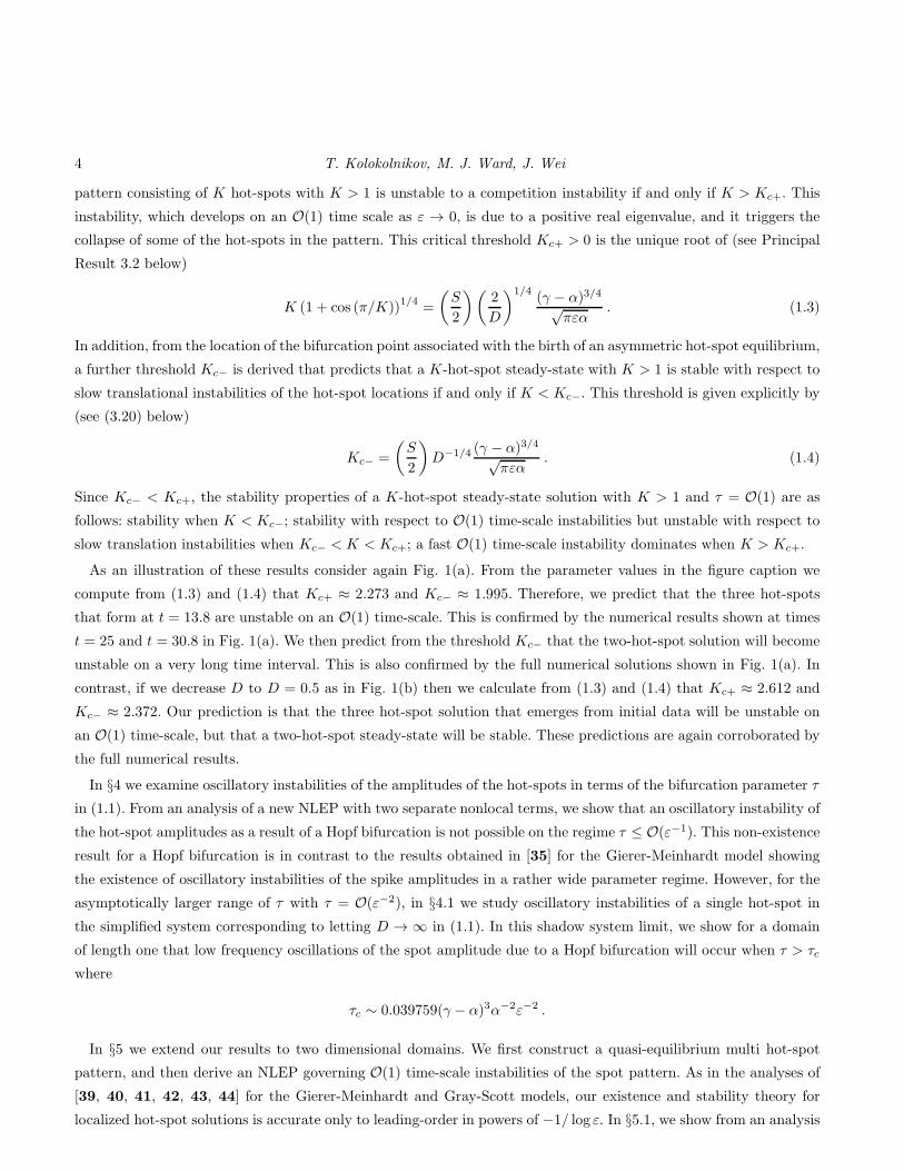
Principal Result 4.2: There is no value of τc > 0 for which the NLEP of (4.7) has a Hopf bifurcation.
We note that there is a key step in the derivation of Principal Result 4.2 which relies on a numerical computation,
see below. A completely computer-free derivation of this result is still an open problem.
16 T. Kolokolnikov, M. J. Ward, J. Wei
0
0.5
1
1.5
2
2.5
3
2 4 6 8 10 12 14 16 18 20
@@I
ρ(µ) =
∫
w[
(L2
0+µ)
−1]
L0w dy∫
w(L2
0+µ)−1
w dy
∫
w[
(
L20 + µ
)−1]
L0w dy
∫
w(
L20 + µ
)−1w dy
µ
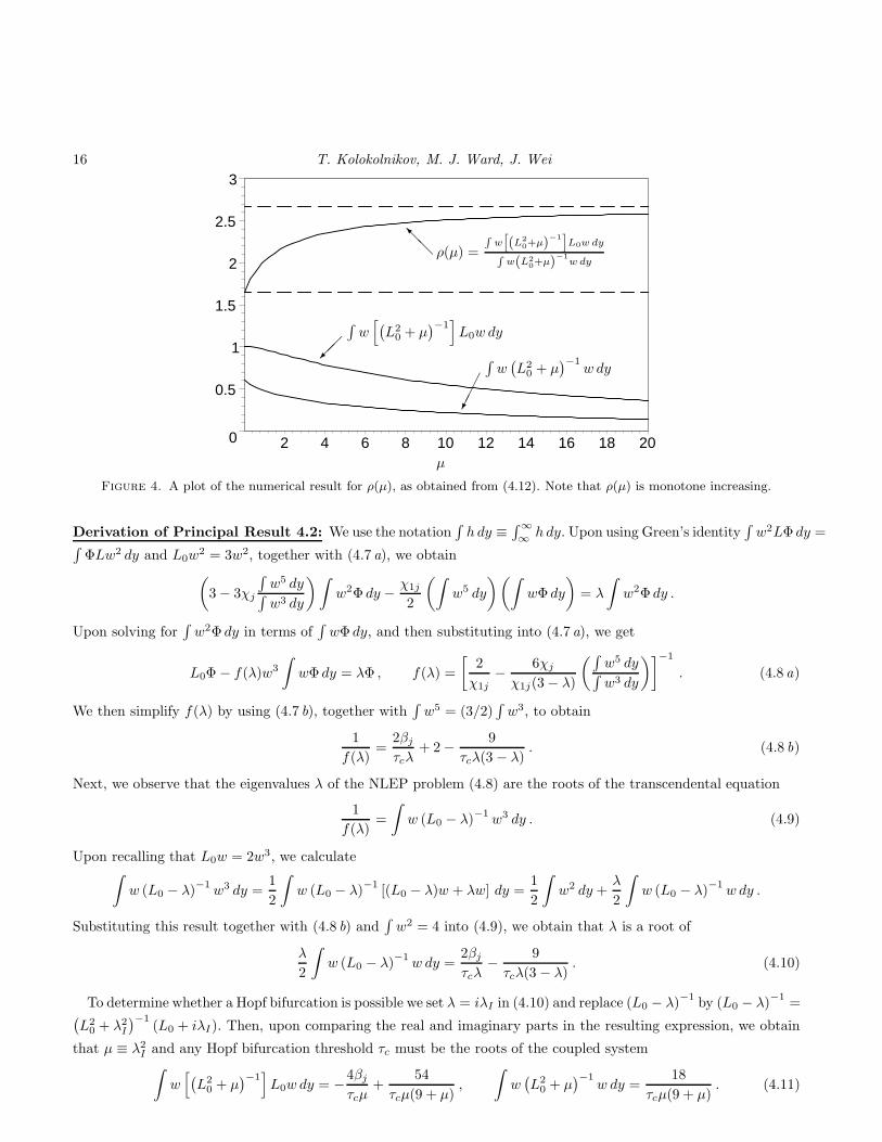
Figure 4. A plot of the numerical result for ρ(µ), as obtained from (4.12). Note that ρ(µ) is monotone increasing.
Derivation of Principal Result 4.2: We use the notation∫
h dy ≡∫∞
∞h dy. Upon using Green’s identity
∫
w2LΦ dy =∫
ΦLw2 dy and L0w2 = 3w2, together with (4.7 a), we obtain
(
3− 3χj
∫
w5 dy∫
w3 dy
)∫
w2Φ dy − χ1j
2
(∫
w5 dy
)(∫
wΦ dy
)
= λ
∫
w2Φ dy .
Upon solving for∫
w2Φ dy in terms of∫
wΦ dy, and then substituting into (4.7 a), we get
L0Φ− f(λ)w3
∫
wΦ dy = λΦ , f(λ) =
[
2
χ1j− 6χj
χ1j(3− λ)
(∫
w5 dy∫
w3 dy
)]−1
. (4.8 a)
We then simplify f(λ) by using (4.7 b), together with∫
w5 = (3/2)∫
w3, to obtain
1
f(λ)=
2βjτcλ
+ 2− 9
τcλ(3 − λ). (4.8 b)
Next, we observe that the eigenvalues λ of the NLEP problem (4.8) are the roots of the transcendental equation
1
f(λ)=
∫
w (L0 − λ)−1w3 dy . (4.9)
Upon recalling that L0w = 2w3, we calculate∫
w (L0 − λ)−1w3 dy =
1
2
∫
w (L0 − λ)−1
[(L0 − λ)w + λw] dy =1
2
∫
w2 dy +λ
2
∫
w (L0 − λ)−1w dy .
Substituting this result together with (4.8 b) and∫
w2 = 4 into (4.9), we obtain that λ is a root of
λ
2
∫
w (L0 − λ)−1w dy =
2βjτcλ
− 9
τcλ(3 − λ). (4.10)
To determine whether a Hopf bifurcation is possible we set λ = iλI in (4.10) and replace (L0 − λ)−1
by (L0 − λ)−1
=(
L20 + λ2I
)−1(L0 + iλI). Then, upon comparing the real and imaginary parts in the resulting expression, we obtain
that µ ≡ λ2I and any Hopf bifurcation threshold τc must be the roots of the coupled system∫
w[
(
L20 + µ
)−1]
L0w dy = −4βjτcµ
+54
τcµ(9 + µ),
∫
w(
L20 + µ
)−1w dy =
18
τcµ(9 + µ). (4.11)
The Stability of Steady-State Hot-Spot Patterns for a Reaction-Diffusion Model of Urban Crime 17
Upon eliminating τc from (4.11), we obtain a transcendental equation solely for µ = λ2I > 0,
ρ(µ) = 3− 2βj − 2βj9µ , where ρ(µ) ≡
∫
w[
(
L20 + µ
)−1]
L0w dy∫
w (L20 + µ)
−1w dy
. (4.12)
By using the identities L0w = 2w3 and L−10 w = (w + yw′) /2, the limiting behavior for ρ(µ) is readily calculated as
ρ (∞) =
∫
wL0w dy∫
w2 dy=
8
3; ρ(0) =
∫
wL−10 w dy
∫ (
L−10 w
)2dy
=36
π2 + 12≈ 1.6461 .
Moreover, direct numerical computations of ρ(µ) show that it is an increasing function of µ (see Fig. 4). On the
other hand, for µ > 0 we have 3− 2βj − 2βj
9 µ < 1 since βj ≥ 1. It follows that (4.12) cannot have any solution with
µ > 0. Consequently, there is no Hopf bifurcation on the parameter regime τ = O(ε−1).
Such a non-existence result for Hopf bifurcations for the crime model when τ = O(ε−1) is qualitatively very
different than for the Gierer-Meinhardt and Gray-Scott models, analyzed in [35] and [15], where Hopf bifurcations
occur in wide parameter regimes.
4.1 A Hopf Bifurcation for the Shadow Limit
Principal Result 4.2 has shown that there is no Hopf bifurcation for the regime τ = O(ε−1). However, a Hopf
bifurcation can and does appear when τ = O(ε−2). As will be shown below, in such a regime the amplitude of the
hot-spot becomes oscillatory with an asymptotically large temporal period, due to an eigenvalue that is dominated,
to leading-order in ε, by its pure imaginary part. To illustrate this phenomenon, in this section we analytically derive
the condition for a Hopf bifurcation of a single boundary spot on a domain of length one. To further simplify our
computations, we will assume thatD0 in (2.5 b) is taken sufficiently large such that v(x, t) = v(t) can be approximated
by a time-dependent constant. The limit D → ∞ is called the shadow-limit (cf. [38]). Our main result is the following:
Principal Result 4.3: Suppose that D0 ≫ 1 and consider a half hot-spot of (2.5) located at the origin on the domain
[0, 1], as constructed in Principal Result 2.1. Define τ0c by
τ0c =
(
24− π2)
36π2
(γ − α)3
α2= 0.039769
(γ − α)3
α2. (4.13)
Let τ = τ0/ε2. Then, there is a Hopf bifurcation at τ0 = τ0c. That is, the hot spot is stable for τ0 < τ0c and is
unstable for τ0 > τ0c. Destabilization takes place via a Hopf bifurcation. More precisely, when τ0 = O(1), the related
stability problem has an eigenvalue near the origin with the following asymptotic behavior as ε→ 0:
λ ∼
±√
γ − α
τ0
iε1/2 +
α2π2
2(γ − α)2− (γ − α)
τ0
(
24− π2
72
)
ε . (4.14)
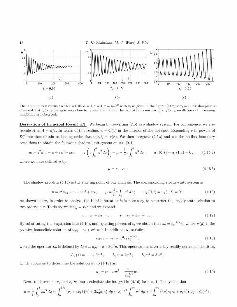
Numerical example. To illustrate Principal Result 4.3 we take γ = 4, α = 1, ε = 0.05 and D0 = 1000. Then,
(4.13) yields τ0c ≈ 1.07378. Now take τ0 = 0.95 so that (4.14) yields the eigenvalue λ ≈ 0.4082i− 0.00529. We then
expect the single hot-spot to be stable, although it will exhibit long transient oscillations. From the eigenvalue, we
can estimate the period of the oscillation to be P = 2π0.4082 ≈ 15.39. This agrees with full numerical solutions of (4.15)
as shown in Fig. 5(a).
Next, we increase τ0 to 1.15, while keeping the other parameters the same. In this case, τ0 > τ0c so that the
hot-spot is unstable in the limit ε → 0. However, τ0 = 1.15 is very close to the threshold value, and with ε = 0.05,
we expect even longer transients with the final state still unclear at t = 300. This behavior is shown in Fig. 5(b).
Finally, as shown in Fig. 5(c), when we increase τ0 to 1.35, we clearly observe oscillations of an increasing amplitude.
18 T. Kolokolnikov, M. J. Ward, J. Wei
(a) (b) (c)
Figure 5. max u versus t with ε = 0.05, α = 1, γ = 4, τ = τ0/ε2 with τ0 as given in the figure. (a) τ0 < τc = 1.074; damping is
observed. (b) τ0 > τc but τ0 is very close to τc; eventual fate of the oscillation is unclear. (c) τ0 > τc; oscillations of increasingamplitude are observed.
Derivation of Principal Result 4.3: We begin by re-writing (2.5) as a shadow system. For convenience, we also
rescale A as A = u/ε. In terms of this scaling, u = O(1) in the interior of the hot-spot. Expanding v in powers of
D−10 we then obtain to leading order that v(x, t) ∼ v(x). We then integrate (2.5 b) and use the no-flux boundary
conditions to obtain the following shadow-limit system on x ∈ [0, 1]:
ut = ε2uxx − u+ vu3 + εα , τ
(
v
∫ 1
0
u2 dx
)
t
= µ− 1
εv
∫ 1
0
u3 dx ; ux (0, t) = ux(1, t) = 0 , (4.15 a)
where we have defined µ by
µ ≡ γ − α . (4.15 b)
The shadow problem (4.15) is the starting point of our analysis. The corresponding steady-state system is
0 = ε2uxx − u+ vu3 + εα , µ =1
εv
∫ 1
0
u3 dx ; ux (0, t) = ux(1, t) = 0 . (4.16)
As shown below, in order to analyze the Hopf bifurcation it is necessary to construct the steady-state solution to
two orders in ε. To do so, we let y = x/ε and we expand
u = u0 + εu1 . . . , v = v0 + εv1 + . . . . (4.17)
By substituting this expansion into (4.16), and equating powers of ε, we obtain that u0 = v−1/20 w, where w(y) is the
positive homoclinic solution of wyy − w + w3 = 0. In addition, u1 satisfies
L0u1 = −α− w3v1v−3/20 , (4.18)
where the operator L0 is defined by L0u ≡ uyy −u+3w2u. This operator has several key readily derivable identities,
L0 (1) = −1 + 3w2 , L0w = 2w3 , L0w2 = 3w2 ,
which allows us to determine the solution u1 to (4.18) as
u1 = α− αw2 − v1
2v3/20
w . (4.19)
Next, to determine v0 and v1 we must calculate the integral in (4.16) for ε≪ 1. This yields that
µ =1
ε
∫ 1
0
vu3 dx ∼∫ 1/ε
0
(v0 + εv1)(
u30 + 3u20u1ε)
dy ∼ v−1/20
∫ ∞
0
w3 dy + ε
∫ ∞
0
(
3u20u1v0 + v1u30
)
dy +O(ε2) .
The Stability of Steady-State Hot-Spot Patterns for a Reaction-Diffusion Model of Urban Crime 19
By equating coefficients of ε, we get that v0 and v1 satisfy
v−1/20
∫ ∞
0
w3dy = µ ,
∫ ∞
0
3u1w2 dy + v1v
−3/20
∫ ∞
0
w3 dy = 0 .
Upon using the solution (4.19) for u1, the unknown v1 can be determined in terms of a quadrature as
v1 = 6αv3/20
∫∞
0
(
w2 − w4)
dy∫∞
0 w3 dy.
The integrals defining v0 and v1 are then calculated explicitly by using
w =√2 sech y ,
∫ ∞
−∞
w2 dy = 4 ,
∫ ∞
−∞
w3 dy =
∫ ∞
−∞
w dy =√2π ,
∫ ∞
−∞
w4 dy =16
3,
which yields the explicit formulae
v0 =π2
2µ−2 , v1 = −2απ2µ−3 . (4.20)
Next, we study the stability of this solution. For convenience, we extend the problem to the interval [−1, 1] by
even reflection. We linearize (4.15) around the steady-state solution to obtain the eigenvalue problem
λφ = ε2φ′′ − φ+ 3u2vφ+ u3ψ ; τλ
∫ 1/ε
−1/ε
(
2φuv + u2ψ)
dy =−1
ε
∫ 1/ε
−1/ε
(
3u2vφ + u3ψ)
dy ,
where the constant ψ denotes the perturbation in v. Upon solving for ψ we obtain
ε2φ′′ − φ+ 3u2vφ+ u3ψ = λφ ; ψ = −τλε
∫ 1/ε−1/ε2φuv dy +
∫ 1/ε−1/ε3u
2vφ dy
τλε∫ 1/ε−1/εu
2 dy +∫ 1/ε−1/εu
3 dy. (4.21)
To motivate the analysis below, we first suppose that τλε ≫ 1. Then, by using u ∼ w/√v0 and v ∼ v0 , (4.21)
reduces to leading order to the NLEP
L0φ− 2w3
∫
φw∫
w2= λφ .
Here and below,∫
f denotes∫∞
−∞fdy. This problem has a zero eigenvalue corresponding to the eigenfunction φ = w.
All other discrete eigenvalues satisfy Re(λ) < 0 (cf. [46]). Therefore, the critical eigenvalue will be a perturbation of
the zero eigenvalue.
A posteriori computations shows that the correct anzatz is in fact
λ = ε1/2λ0 + ελ1 + . . . ; τ = τ0ε−2 .
The analysis below shows that λ0 is purely imaginary, and hence determines the frequency of the oscillation, but
not its stability. Therefore, a two-term expansion in λ must be obtained in order to determine the stability of the
oscillations. As such, we must expand all quantities in the shadow problem up to O(ε). The delicate part in the
calculation is to note that∫ 1/ε
−1/εu2 =
∫
u20 + ε
∫
2u0u1 + ε2∫ 1/ε
−1/ε
u21 ,
where the last integral is in fact O(ε) as a result of
ε2∫ 1/ε
−1/εu21 = ε2
∫ 1/ε
−1/ε
(α+ . . .)2 = 2α2ε+ . . .
Thus, this term “jumps” an order and is comparable in magnitude to ε∫
2u0u1. The remaining part of the analysis
20 T. Kolokolnikov, M. J. Ward, J. Wei
is more straightforward. We let τ = τ0ε−2 and expand ψ in (4.21) as
ψ = −τλε∫
2φuv +∫
3u2vφ
τλε∫
u2 +∫
u3= ψ0 + ε1/2ψ1/2 + εψ1 ,
so that the eigenvalue problem for φ from (4.21) becomes
(ε1/2λ0 + ελ1)φ = L0φ+ (3u20v1 + 6u0u1v0)φε+ u30
(
ψ0 + ε1/2ψ1/2 + εψ1
)
+ 3u20u1ψ0ε
= L1φ+ ε1/2L2φ+ εL3φ . (4.22)
After tedious but straightforward computations, the three operators in (4.22) are given by
L1φ ≡ L0φ− 2
∫
wφ∫
w2w3 ; (4.23 a)
L2φ ≡ ψ1/2u30 =
(
c0
∫
wφ+ c1
∫
w2φ
)
w3 ; (4.23 b)
L3φ ≡ (3u20v1 + 6u0u1v0)φ+ 3u20u1ψ0 + u30ψ1
=(
c2w + c3w2 + c4w
3)
φ+(
c5w2 + c6w
3 + c7w4)
∫
wφ+ c8w3
∫
φ+ c9w3
∫
w2φ , (4.23 c)
in terms of the coefficients c0, . . . , c9 defined by
c0 =µ
4τ0λ0; c1 = − 3µ
√2
4πτ0λ0; c2 =
3πα√2
µ; c3 = 0 ; c4 = −c2 ; c5 = −3
√2πα
4µ
c6 = − µλ14τ0λ20
− µ2
8τ20λ20
+π2α2
8µ2; c7 = −c5 ; c8 = −π
√2α
4µ; c9 =
√2πα
4µ+
√23µλ1
4πτ0λ20+
√23µ2
8πτ20λ20
. (4.24)
Finally, we expand φ in (4.22) as
φ = w + ε1/2φ1 + εφ2 ,
and equate powers of ε in (4.22). This yields the following problems for φ1 and φ2:
λ0w = L1φ1 + L2w , (4.25)
λ1w + λ0φ1 = L1φ2 + L2φ1 + L3w . (4.26)
To determine λ0 and φ1 we must formulate the appropriate solvability condition based on the adjoint operator L∗1
of L1 defined by
L∗
1φ ≡ L0φ− 2
∫
w3φ∫
w2w . (4.27)
Since L1 admits a zero eigenvalue of multiplicity one, then so does L∗1. In fact, w∗ defined by
w∗ ≡ (ywy + w) /2 , (4.28)
is the unique element in the kernel of L∗1, i.e. L
∗1w
∗ = 0, owing to the following two readily derived identities:
L0w∗ = w , 2
∫
w3w∗
∫
w2= 1 . (4.29)
Next, we impose a solvability condition on (4.25) in the usual way. We multiply (4.25) by w∗ and integrate by
parts to derive that
λ0 =
∫
w∗L2w∫
w∗w=
(
c0
∫
w2 + c1
∫
w3
)∫
w∗w3
∫
w∗w= 2
(
c0
∫
w2 + c1
∫
w3
)
, (4.30)
The Stability of Steady-State Hot-Spot Patterns for a Reaction-Diffusion Model of Urban Crime 21
where we used the integral identity in (4.29) together with∫
w∗w =∫
w2/4. From the formulae for the coefficients
c0 and c1 in (4.24), (4.30) determines λ0 as
λ0 = ±i√
µ
τ0. (4.31)
Since λ0 is purely imaginary, the next order term λ1 needs to be computed to determine stability.
The problem (4.25) for φ1 can be written by using (4.23a) and (4.23 b) as
L0φ1 = λ0w −(
c0
∫
w2 + c1
∫
w3 + 2
∫
wφ1∫
w2
)
w3 .
Since L0w∗ = w and L0w = 2w3, we can write φ1 as
φ1 = λ0w∗ − dw
2where d ≡ c0
∫
w2 + c1
∫
w3 + 2
∫
wφ1∫
w2. (4.32)
Upon substituting φ1 into the definition of d, we can then solve for d by using (4.30) for λ0 to get
2d = c0
∫
w2 + c1
∫
w3 + 2λ0
∫
ww∗
∫
w2= c0
∫
w2 + c1
∫
w3 + 2
(
c0
∫
w2 + c1
∫
w3
)∫
w∗w3
∫
w2.
Finally, by using∫
w∗w =∫
w2/4, the expression above simplifies to
d = c0
∫
w2 + c1
∫
w3
so that φ1 is given explicitly from (4.32) as
φ1 =
(
c0
∫
w2 + c1
∫
w3
)
(
2w∗ − w
2
)
. (4.33)
With φ1 explicitly known, we impose the solvability condition on the problem (4.26) for φ2 to determine λ2 as
λ1 =
∫
w∗ (L2 − λ0)φ1 +∫
w∗L3w∫
w∗w.
Upon using (4.33) for φ1, L3w from (4.23 c), and (L2 − λ0) from (4.23 b), the integrals above are evaluated as
λ1 =
(
−16π2
9− 16
3
)
c20 +
(
−4
3
√2π − 8
9
√2π3
)
c1c0 −2π4
9c21
+
√2π
3c2 +
3√2π
5c4 +
4√2π
3c5 + 8c6 +
12√2π
5c7 + 2
√2c8π + 2
√2πc9 .
Finally, upon substituting c0, . . . , c9 from (4.24) into this expression, we determine λ1 explicitly as
λ1 =α2π2
2µ2− µ
τ0
(
24− π2
72
)
(4.34)
The two-term expansion for λ given in (4.14) follows from (4.31) and (4.34). The Hopf bifurcation threshold is
obtained by setting λ1 = 0. This occurs precisely as τ0 is increased past τ0c, where τc is given by (4.13).
5 Hot-Spot Patterns in 2-D: Equilibria and Stability
In this section we construct a K-spot quasi-steady-state solution to (1.1) in an arbitrary 2-D domain with spots
centered at x1, . . . , xK . To leading-order in σ = −1/ log ε, we then derive a threshold condition on the diffusivity D
for the stability of the K-spot quasi-steady-state solution to instabilities that develop on an O(1) time-scale.
22 T. Kolokolnikov, M. J. Ward, J. Wei
As in the analysis of hot-spot patterns in one spatial dimension, we set V = P/A2 (see (2.2)) into (1.1) to obtain
At = ε2∆A−A+ V A3 + α , x ∈ Ω ; ∂nA = 0 , x ∈ ∂Ω , (5.1 a)
τ(
A2V)
t= D∇ ·
(
A2∇V)
− V A3 + γ − α , x ∈ Ω ; ∂nV = 0 , x ∈ ∂Ω . (5.1 b)
We first motivate the ε-dependent re-scalings of V and A that are needed for the 2-D case. We suppose that
D ≫ 1, so that V is approximately constant. By integrating the steady-state equation of (5.1 b) over Ω we get
V = c/∫
ΩA3 dx, where c is some O(1) constant. Therefore, if A = O(ε−p) in the inner hot-spot region of area O(ε2),
we obtain∫
ΩA3 dx = O(ε2−3p), so that V = O(ε3p−2). In addition, from the steady-state of (5.1 a), we must have in
the inner region that A3V ∼ A, so that −3p+ (3p− 2) = −p. This yields p = 2. Therefore, for D ≫ 1, V = O(ε4)
globally on Ω, while A = O(ε−2) in the inner region near a hot-spot. Finally, in the outer region we must have
A ∼ α = O(1), so that from (5.1 b), we conclude that D∇ ·(
A2∇V)
∼ α− γ = O(1). Since V = O(ε4), this balance
requires that D = O(ε−4). Finally, in the core of a hot-spot we conclude that the density P of criminals, given by
P = V A2, is O(1) as ε→ 0.
Although this simple scaling analysis correctly identifies the algebraic factors in ε, there are more subtle logarithmic
terms of the form σ ≡ −1/ log ε that are needed in the construction of the quasi-steady-state hot spot solution.
The scaling analysis above motivates the introduction of new variables v, u, and D defined by
V = ε4v , A = ε−2u , D = D/ε4 . (5.2)
In terms of (5.2), (5.1) transforms exactly to
ut = ε2∆u− u+ vu3 + αε2 , x ∈ Ω ; ∂nu = 0 , x ∈ ∂Ω , (5.3 a)
τ(
u2v)
t=
Dε4
∇ ·(
u2∇v)
− ε−2vu3 + γ − α , x ∈ Ω ; ∂nv = 0 . x ∈ ∂Ω . (5.3 b)
Owing to the non-uniformity in the behavior as |y| → ∞ of the solution to this core problem near a spot (see
below), the construction of a quasi-steady-state K-spot solution for (5.3) is more intricate than that for the Gierer-
Meinhardt, Schnakenburg, or Gray-Scott problems analyzed in [39]–[44], [13], [16], and [1]. As such, we will only
develop a theory that is accurate to leading order in σ ≡ −1/ log ε, similar to that undertaken in [39]–[44], and
[13]. This is in contrast to the recent approach in [16] and [1] that used a hybrid asymptotic-numerical method to
construct quasi-steady-state spot patterns to the Schnakenburg and Gray-Scott systems, respectively, with an error
that is beyond-all-orders with respect to σ.
In the outer region, away from the spots centered at x1, . . . , xK , we expand u and v as
u = αε2 + o(ε2) , v ∼ h0 + σh1 + · · · , (5.4)
where σ = −1/ log ε and D = D0/σ, where D0 = O(1). From the steady-state of (5.3 b) we obtain that h0 is constant,
and that h1 satisfies
∆h1 = − (γ − α)
α2D0, x ∈ Ω\x1, . . . , xK ; ∂nh1 = 0 , x ∈ Ω . (5.5)
As shown below, this problem must be augmented by certain singularity conditions that are obtained by matching
the outer solution for v to certain inner solutions, one in the neighborhood of each spot.
In the inner region near the j-th spot centered at xj we introduce the inner variables y, uj, and vj by
y = ε−1(x− xj) , vj(y) = v(xj + εy) , uj(y) = u(xj + εy) . (5.6)
The Stability of Steady-State Hot-Spot Patterns for a Reaction-Diffusion Model of Urban Crime 23
In terms of these inner variables, and with D = σ−1D0, the steady-state of (5.3) transforms exactly on y ∈ R2 to
∆yuj − uj + vju3j + αε2 = 0 , (5.7 a)
∇y ·(
u2j∇yvj)
− ε4σ
D0vju
3j = −ε
6σ
D0(γ − α) , (5.7 b)
where σ ≡ −1/ log ε. We will construct a radially symmetric solution uj = uj(ρ), vj = vj(ρ) to this problem, where
ρ = |y|.The complication in analyzing (5.7) is that uj = O(1) for |y| = O(1), whereas uj = O(ε2) for |y| ≫ 1. Therefore,
the “diffusivity” u2j in the operator for v in (5.7 b) ranges from O(1) when |y| = O(1) to O(ε4) when |y| ≫ 1. For
this reason, we cannot simply neglect the second term on the left-hand side of (5.7 b) for all |y|. However, as we showbelow, we can neglect the O(ε6) term on the right-hand side of (5.7 b).
For |y| = O(1), we expand uj and vj as
uj = uj0 + ε2uj1 + · · · , vj = vj0 + ε2vj1 + · · · . (5.8)
Upon substituting this expansion into (5.7), we obtain that vj0 and vj1 are constants, and that uj0 and uj1 are
radially symmetric solutions of
∆ρuj0 − uj0 + vj0u3j0 = 0 , ∆ρuj1 − uj1 + 3u2j0vj0uj1 = −α− u3j0vj1 ,
on ρ ≥ 0 with uj0 → 0 and uj1 → α as ρ → ∞. Here ∆ρg ≡ g′′ + ρ−1g′ for g = g(ρ). In terms of the unknown
constants vj0 and vj1, the solutions for uj0 and uj1 are
uj0 = v−1/2j0 w , uj1 = α− vj1
2v3/2j0
w − 3αw1 , (5.9)
where w = w(ρ) and w1 = w1(ρ) are the unique radially symmetric solutions of
∆ρw − w + w3 = 0 , Lw1 ≡ ∆ρw1 − w1 + 3w2w1 = w2 , (5.10)
with w(ρ) > 0, w′(0) = 0, and w → 0 as ρ → ∞, together with w′1(0) = 0 and w1 → 0 as ρ → ∞. The expression
(5.9) for uj1 shows that uj1 → α as ρ→ ∞, so that from (5.8) uj ∼ αε2 when |y| ≫ 1.
Next, we calculate the far-field behavior, valid for |y| ≫ 1, for the solution vj to (5.7 b). To do so, we define the
ball Bδ = y | |y| ≤ δ, where 1 ≪ δ ≪ O(ε−1). Therefore, this ball is defined in the intermediate matching region
between the inner and outer scales y and x, respectively. Upon integrating (5.7 b) over Bδ, and using the divergence
theorem, we obtain that
2πu2jδv′
j |ρ=δ ∼ ε4σ
D0
∫
Bδ
vju3j dy +O(δ2σε6) . (5.11)
Since uj = O(1) only for |y| = O(1) where vj ∼ vj0 + o(1), the integral on the right hand-side of (5.11) can be
estimated by using uj ∼ v−1/2j0 w. In contrast, on the left hand-side of (5.11) we use uj ∼ αε2 on ρ = δ ≫ 1. In this
way, we obtain that (5.11) becomes
2πα2δε4v′j |ρ=δ ∼(
2πε4σ√vj0 D0
)∫ ∞
0
w3 ρ dρ+O(δ2σε6) . (5.12)
Since δ ≪ O(ε−1), we can neglect the last term on the right hand-side of (5.12), which is equivalent to neglecting
the right-hand side of (5.7 b) for the inner problem.
24 T. Kolokolnikov, M. J. Ward, J. Wei
From (5.12) we obtain that the far-field behavior for |y| ≫ 1 for the solution to (5.7 b) has the form
vj ∼ vj0 + σ (Sj log |y|+O(1)) , (5.13 a)
where Sj is defined by
Sj ≡b
α2D0√vj0
, b ≡∫ ∞
0
w3ρ dρ . (5.13 b)
Therefore, the appropriate core problem determining the asymptotic shape of the hot-spot profile is to seek a radially
symmetric solution to
∆yuj − uj + vju3j + αε2 = 0 , ∇y ·
(
u2j∇yvj)
=ε4σ
D0vju
3j . (5.14)
The next step in the construction of the multi hot-spot quasi-steady-state pattern is to match the inner and outer
solutions for v in order to determine vj0. We let y = ε−1(x − xj) in (5.13a) to obtain that the outer solution for v
must have the singularity behavior
v ∼ vj0 + Sj + σ [Sj log |x− xj |+O(1)] , as x→ xj , j = 1, . . . ,K . (5.15)
Upon comparing (5.15) with the outer expansion v ∼ h0 + σh1 + · · · from (5.4), we conclude that
h0 = vj0 + Sj , j = 1, . . . ,K , (5.16 a)
and that h1 satisfies (5.5) subject to the singularity behaviors
h1 ∼ Sj log |x− xj |+O(1) , as x→ xj , j = 1, . . . ,K . (5.16 b)
Upon using the divergence theorem, the problem for h1 has a solution only when the solvability condition
K∑
j=1
Sj =(γ − α)
2πα2D0|Ω| , (5.16 c)
is satisfied, where |Ω| is the area of Ω. When this condition is satisfied, the solution for h1 can be written as
h1 = −2πK∑
i=1
SiG(x;xi) + h1 , (5.17)
where h1 is a constant to be determined, and where G(x;xi) is the Neumann Green’s function satisfying
∆G =1
|Ω| − δ(x− xi) , x ∈ Ω ; ∂nG = 0 , x ∈ ∂Ω , (5.18 a)
∫
Ω
G(x;xi) dx = 0 ; G ∼ − 1
2πlog |x− xi|+O(1) , as x→ xi . (5.18 b)
In summary, the asymptotic matching provides the following algebraic system for determining vj0 for j = 1, . . . ,K:
h0 = F(vj0) ≡ vj0 +c
√vj0
,
K∑
j=1
v−1/2j0 =
|Ω|(γ − α)
2πb, c ≡ b
α2D0. (5.19)
A symmetric K-hot-spot quasi-steady-state solution corresponds to a solution of (5.19) for which vj0 = v0 for all j.
From (5.9), this solution is characterized by the fact that the hot-spot profile is, to leading-order, the same for each
j. The result for such symmetric quasi-equilibria is summarized as follows:
Principal Result 5.1: For ε → 0, a symmetric K-hot-spot quasi-steady-state solution to (5.3) on the parameter
The Stability of Steady-State Hot-Spot Patterns for a Reaction-Diffusion Model of Urban Crime 25
0
0.1
0.2
0.3
0.4
0.5
u(r)
0.2 0.4 0.6 0.8 1r23
23.05
23.1
23.15
23.2
23.25
23.3
23.35
23.4
v(r)
0 0.2 0.4 0.6 0.8 1r
(a) (b)
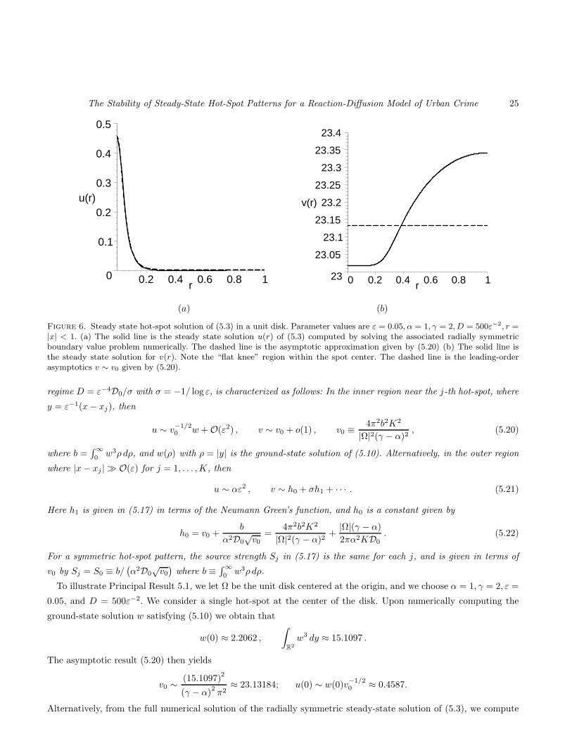
Figure 6. Steady state hot-spot solution of (5.3) in a unit disk. Parameter values are ε = 0.05, α = 1, γ = 2, D = 500ε−2, r =|x| < 1. (a) The solid line is the steady state solution u(r) of (5.3) computed by solving the associated radially symmetricboundary value problem numerically. The dashed line is the asymptotic approximation given by (5.20) (b) The solid line isthe steady state solution for v(r). Note the “flat knee” region within the spot center. The dashed line is the leading-orderasymptotics v ∼ v0 given by (5.20).
regime D = ε−4D0/σ with σ = −1/ log ε, is characterized as follows: In the inner region near the j-th hot-spot, where
y = ε−1(x− xj), then
u ∼ v−1/20 w +O(ε2) , v ∼ v0 + o(1) , v0 ≡ 4π2b2K2
|Ω|2(γ − α)2, (5.20)
where b =∫∞
0w3ρ dρ, and w(ρ) with ρ = |y| is the ground-state solution of (5.10). Alternatively, in the outer region
where |x− xj | ≫ O(ε) for j = 1, . . . ,K, then
u ∼ αε2 , v ∼ h0 + σh1 + · · · . (5.21)
Here h1 is given in (5.17) in terms of the Neumann Green’s function, and h0 is a constant given by
h0 = v0 +b
α2D0√v0
=4π2b2K2
|Ω|2(γ − α)2+
|Ω|(γ − α)
2πα2KD0. (5.22)
For a symmetric hot-spot pattern, the source strength Sj in (5.17) is the same for each j, and is given in terms of
v0 by Sj = S0 ≡ b/(
α2D0√v0)
where b ≡∫∞
0w3ρ dρ.
To illustrate Principal Result 5.1, we let Ω be the unit disk centered at the origin, and we choose α = 1, γ = 2, ε =
0.05, and D = 500ε−2. We consider a single hot-spot at the center of the disk. Upon numerically computing the
ground-state solution w satisfying (5.10) we obtain that
w(0) ≈ 2.2062 ,
∫
R2
w3 dy ≈ 15.1097 .
The asymptotic result (5.20) then yields
v0 ∼ (15.1097)2
(γ − α)2π2
≈ 23.13184; u(0) ∼ w(0)v−1/20 ≈ 0.4587.
Alternatively, from the full numerical solution of the radially symmetric steady-state solution of (5.3), we compute
26 T. Kolokolnikov, M. J. Ward, J. Wei
that v(0) ≈ 23.017 and u(0) ≈ 0.455. The error is about 0.5% for v(0) and about 0.8% for u(0). A comparison of
asymptotic and numerical results is shown in Fig. 6.
As a remark, the general shape of the function F(v) defined in (5.19) also shows that there can be asymmetric
K-spot quasi-equilibria corresponding to spots of two distinct heights. Similar asymmetric patterns in 2-D have been
constructed for the Gierer-Meihnardt and Gray-Scott systems in [43]) and ([44]. Let Ks and Kb be non-negative
integers denoting the number of small and large spots, respectively, with K = Ks +Kb. Then, from (5.19), a K-spot
asymmetric pattern is constructed by determining two distinct values v0s and v0b satisfying
F(v0l) = F(v0r) , v0b < vmin < v0s ,Ks√v0s
+Kb√v0b
=|Ω|(γ − α)
2πb, (5.23)
where vmin = 3 (c/2)3/2
and c is defined in (5.19). The spatial profile of the hot-spot of large and small amplitude is
given by u ∼ v−1/20s w and u ∼ v
−1/20b w, respectively.
We will not investigate the solvability with respect to D0 of the algebraic system (5.23) governing asymmetric
spot patterns. Instead, in the next subsection we will study the stability properties of the symmetric K-hot-spot
quasi-steady-state solution given in Principal Result 5.1.
5.1 The Stability of Hot-Spot Quasi-Steady-State Patterns
We linearize (5.3) around the quasi-steady-state K-hot-spot pattern to obtain the eigenvalue problem
ε2∆φ− φ+ 3u2v φ+ u3 ψ = λφ , x ∈ Ω ; ∂nφ = 0 , x ∈ ∂Ω , (5.24 a)
D∇ ·(
u2∇ψ + 2uφ∇v)
− 1
ε2(
3u2v φ+ u3 ψ)
= τλ(
u2ψ + 2uvφ)
, x ∈ Ω ; ∂nψ = 0 , x ∈ ∂Ω . (5.24 b)
In our stability analysis we will consider the range of D where D = ε−4D0/σ and D0 = O(1). It is on this parameter
range of D that a stability threshold occurs. Our main stability result is as follows:
Principal Result 5.2: Consider the K-spot quasi-steady-state solution of (5.3) as constructed in Principal Result
5.1 for ε ≪ 1. Assume that τ = τ0/ε2 where τ0 = O(1). Then, for ε→ 0, and to leading order in σ = −1/ log ε, the
stability on an O(1) time-scale of a K-hot-spot quasi-steady-state solution with K ≥ 2 is determined by the spectrum
of the two distinct NLEP’s
∆yΦ− Φ+ 3w2Φ− κiw3
[
∫
R2 w2Φ dy
∫
R2 w3 dy+
2
3τ0λβ
∫
R2 wΦ dy∫
R2 w2 dy
]
= λΦ , y ∈ R2 , (5.25 a)
with Φ → 0 as |y| → ∞. Here κi for i = 1, 2 are defined by
κ1 ≡ 3 (1 + τ0λβ)−1
, κ2 ≡ 3
(
1 + τ0λβ +D0
2D0c
)−1
, (5.25 b)
in terms of the constants β and D0c defined by
β ≡ K∫
R2 w2 dy
|Ω|(γ − α), D0c ≡
|Ω|3 (γ − α)3
4πα2K3(∫
R2 w3 dy)2 . (5.25 c)
For a one-hot-spot solution, for which K = 1, there is only a single NLEP with κi in (5.25 a) replaced by κ1. For
τ0 ≪ 1, which is equivalent to τ ≪ O(ε−2), we conclude that a K-spot pattern with K ≥ 2 is stable when D0 < D0c
and is unstable when D0 > D0c. In terms of the unscaled D, this yields the stability threshold
D =
(
ε−4
σ
)
D0c , for K ≥ 2 , σ = −1/ log ε . (5.26)
The Stability of Steady-State Hot-Spot Patterns for a Reaction-Diffusion Model of Urban Crime 27
For K = 1 and τ0 ≪ 1, a single hot-spot is stable for all D0 independent of ε.
To show that D0c is the stability threshold of D0 for K ≥ 2, we let τ0 → 0 in (5.25) to obtain the limiting NLEP’s
∆yΦ− Φ + 3w2Φ− κw3
∫
R2 w2Φ dy
∫
R2 w3 dy= λΦ , y ∈ R
2 ; Φ → 0 as |y| → ∞ , (5.27)
where κ can assume either of the two values
κ10 ≡ 3 , κ20 ≡ 3
(
1 +D0
2D0c
)−1
. (5.28)
For (5.27), the rigorous result in Theorem 3 of [45] establishes the existence of an eigenvalue with Re(λ) > 0 whenever
κ < 2. Thus, since κ20 < 2 when D0 > D0c, we conclude that a K-hot-spot quasi-equilibria with K > 2 is unstable
when D0 > D0c. In addition, the result in Theorem 1 of [45] (see the remark following Theorem 1) proves that all
eigenvalues satisfy Re(λ) < 0 when 2 < κ ≤ 6. Since κ10 = 3 and 2 < κ20 < 3 for all D0 < D0c, it follows that the
NLEP for a K-hot-spot quasi-steady-state solution with K ≥ 2 does not have unstable eigenvalues when D0 < D0c.
For K = 1, which corresponds to a one-hot-spot solution, the only choice for κ is κ = κ10 = 3, and so we have
stability for any D0 > 0 independent of ε.
We make two remarks. Firstly, we anticipate that a single hot-spot solution where K = 1 will be stable provided
that D0 is not exponentially large in 1/ε. The analysis to determine this stability threshold in the near-shadow limit
should be similar to that done for the Gierer-Meinhardt model in [14]. Secondly, it is an open question to analyze
(5.25) for τ0 = O(1) to determine if there are any Hopf bifurcations. The analysis of this problem in the 2-D context
is much more difficult than in 1-D since the identity L0w2 = 3w2 for the local operator L0Φ ≡ ∆yΦ−Φ+3w2Φ in R
1
no longer holds in R2. Moreover, since this identity does not hold in the 2-D case, we cannot determine λ explicitly
when τ0 ≪ 1 as was done for the 1-D case in Lemma 3.2.
The stability threshold in Principal Result 5.2 follows once we derive the NLEP (5.25). The derivation of this
NLEP is done in several distinct steps.
We first consider the inner region near the j-th spot and we introduce the new variables y, Φj(y), and Ψj(y) by
y = ε−1(x− xj) , Φj(y) = φ(xj + εy) , Ψj(y) = ψ(xj + εy) .
Then, with D = ε−4D0/σ and σ = −1/ log ε, (5.24) on y ∈ R2 becomes
∆yΦj − Φj + 3u2jvj Φj + u3j Ψj = λΦj , (5.29 a)
∇y ·(
u2j∇yΨj + 2ujΦj∇yvj)
− ε4σ
D0
(
3u2jvj Φj + u3j Ψj
)
=τλε6σ
D0
(
u2jΨj + 2ujvjΦj
)
. (5.29 b)
Since uj = O(1) and ∇yvj = o(1) when |y| = O(1), we obtain from (5.29 b) that Ψj = Ψj0+O(ε2) when |y| = O(1),
where Ψj0 is an unknown constant. Then, with uj ∼ w/√v0 and vj ∼ v0 for |y| = O(1), we obtain from (5.29 a) that
Φj ∼ Φj0 + o(1), where Φj0 satisfies
∆yΦj0 − Φj0 + 3w2Φj0 + v−3/20 w3 Ψj0 = λΦj0 , y ∈ R
2 ; Φj0 → 0 as |y| → ∞ , (5.30)
where w is the radially symmetric ground-state solution satisfying (5.10).
The next step in the analysis is to determine the constant Ψj0 in (5.30). This is done by first determining the
far-field behavior as |y| → ∞ of the solution to (5.29 b). We define the ball Bδ = y | |y| ≤ δ, where 1 ≪ δ ≪ O(ε−1),
28 T. Kolokolnikov, M. J. Ward, J. Wei
and we integrate (5.29 b) over Bδ to obtain
(
2πu2jΨ′
j|ρ=δ + 4πujΦjv′
j |ρ=δ
)
δ =ε4σ
D0
∫
Bδ
(
Ψju3j + 3u2jvjΦj
)
dy +τλε6σ
D0
∫
Bδ
(
Ψju2j + 2ujvjΦj
)
dy . (5.31)
We now estimate the terms in (5.31) for ε≪ 1.
Since the dominant contribution to the integrals on the right hand-side of (5.31) arises from the region where
|y| = O(1), we can asymptotically estimate these integrals by using uj ∼ w/√v0, vj ∼ v0, and Ψj ∼ Ψj0. For the
left hand-side of (5.31) we use uj ∼ αε2 on ρ ≡ |y| = δ ≫ 1 to get
(
2πε4α2Ψ′
j |ρ=δ + 4πε2αv′jΦj |ρ=δ
)
δ ∼ ε4σ
D0
[
Ψj0
v3/20
∫
R2
w3 dy + 3
∫
R2
w2Φj0 dy
]
+τλε6σ
D0
[
Ψj0
v0
∫
R2
w2 dy + 2√v0
∫
R2
wΦj0 dy
]
. (5.32)
Next, we estimate the second term on the left hand-side of (5.32). For |y| ≫ 1, we obtain from the outer limit of
(5.29 a) that −Φj + ε3α6Ψj ∼ λΦj , so that with Ψj ∼ Ψj0 + o(1), we get
Φj ∼ε6α3
1 + λΨj0 , on ρ = |y| = δ ≫ 1 . (5.33)
In addition, from (5.13 a), we estimate that v′j |ρ=δ ∼ σS0/δ, where S0 is defined in Principal Result 5.1. Substituting
this estimate together with (5.33) into (5.32) we obtain
Ψ′
j |ρ=δδ +2α2ε4σS0
(1 + λ)Ψj0 ∼ σ
2πD0α2
[
Ψj0
v3/20
∫
R2
w3 dy + 3
∫
R2
w2Φj0 dy
]
+τλε2σ
2πD0α2
[
Ψj0
v0
∫
R2
w2 dy + 2√v0
∫
R2
wΦj0 dy
]
. (5.34)
From (5.34), and under the assumption that τ = ε−2τ0, where τ0 = O(1), we conclude that Ψj has the far-field
behavior
Ψj ∼ Ψj0 + σ (Bj log |y|+O(1)) , for |y| ≫ 1 , (5.35)
where Bj for j = 1, . . . ,K is defined by
Bj ∼1
2πD0α2
[
Ψj0
v3/20
∫
R2
w3 dy + 3
∫
R2
w2Φj0 dy
]
+τ0λ
2πD0α2
[
Ψj0
v0
∫
R2
w2 dy + 2√v0
∫
R2
wΦj0 dy
]
. (5.36)
Upon writing (5.35) in terms of the outer variable (x−xj) = εy, we obtain that the matching condition for the outer
solution ψ is
ψ ∼ Bj +Ψj0 + σ (Bj log |x− xj |+O(1)) , as x→ xj , j = 1, . . . ,K . (5.37)
Next, we consider the outer region for ψ where |x − xj | = O(1) for j = 1, . . . ,K. In (5.24 b) we use u ∼ αε2,
∇v = O(σ), and φ = O(ε6) from (5.33) to estimate that
D0
σε4∇ ·(
α2ε4∇ψ +O(σε8))
− ε−2(
α3ε6ψ +O(σε10))
= τλ(
α2ε4ψ +O(σε8)ψ)
.
Hence, when τ = ε−2τ0 we obtain that D0∆ψ ∼ τ0λε2σψ. In order to match with (5.37) we must expand the outer
solution for ψ as
ψ = ψ0 + σψ1 + · · · . (5.38)
The Stability of Steady-State Hot-Spot Patterns for a Reaction-Diffusion Model of Urban Crime 29
We then obtain that ψ0 is a constant, given by
ψ0 = Ψj0 +Bj , j = 1, . . . ,K , (5.39)
and that ψ1 satisfies
∆ψ1 = 0 , x ∈ Ω\x1, . . . , xK ; ∂nψ1 = 0 , x ∈ ∂Ω , (5.40 a)
ψ1 ∼ Bj log |x− xj |+O(1) , as x→ xj , j = 1, . . . ,K . (5.40 b)
The solvability condition for (5.40) is that∑K
j=1 Bj = 0. Upon summing (5.39) from j = 1, . . . ,K, we obtain that
Bj = −Ψj0 +1
K
K∑
j=1
Ψj0 , (5.41)
where Bj is given in (5.36).
The final step in the derivation of the NLEP is to solve (5.36) and (5.41) for Ψj0 and substitute the resulting
expression into (5.30). To do so, We introduce the vectors B ≡ (B1, . . . , BK)T
and Ψ ≡ (Ψ01, . . . ,Ψ0K)T, and we
write the system (5.36) and (5.41) in matrix form as
B = c1Ψ0 − c2F0 + c3Ψ0 − c4F1 , B = − (I − E) Ψ0 , (5.42)
where the constants ci for i = 1, . . . , 4 are defined by
c1 ≡ 1
2πD0α2v3/20
∫
R2
w3 dy , c2 ≡ 3c1v3/20 , c3 ≡ τ0λ
2πD0α2v0
∫
R2
w2 dy , c4 ≡ 2v3/20 c3 , (5.43 a)
and the vectors F0 and F1 are defined by
F0 ≡ −∫
R2 w2Φ0 dy
∫
R2 w3 dy, F1 ≡ −
∫
R2 wΦ0 dy∫
R2 w2 dy. (5.43 b)
Here Φ0 ≡ (Φ01, . . . ,Φ0K)T . In (5.42), I is the K ×K identity matrix and the matrix E is defined by E = K−1eeT ,
where e ≡ (1, . . . , 1)T .
By solving (5.42) for Ψ0, and substituting the resulting expression into (5.30), we obtain the vector NLEP
∆yΦ0 − Φ0 + 3w2Φ0 + w3M(
F0 +c4c2F1
)
= λΦ0 , (5.44)
where the matrix M is defined by
M ≡ v−3/20
[
(1 + c1 + c3)
c2I − 1
c2E]−1
. (5.45)
The matrix M−1 is a rank-one update of a scalar multiple of the identity matrix. As such, its spectrum Mω = κω
can readily be calculated as
κ1 =c2
(c1 + c3)v3/20
, ω1 = (1, . . . , 1)T ; κ2 = . . . = κK =c2
(1 + c1 + c3)v3/20
, ωTj e = 0 , j = 2, . . . ,K .
Notice that the eigenvectors corresponding to the matrix eigenvalues κj for j = 2, . . . ,K span the K− 1 dimensional
subspace perpendicular to e = (1, . . . , 1)T . As such, the competition instability modes correspond to j = 2, . . . ,K,
whereas the synchronous instability mode corresponds to κ1 with eigenvector ω1 = (1, . . . , 1)T .
Then, we use the explicit formulae for cj in (5.43 a) and for v0 in (5.20) to write κi for i = 1, 2 as in (5.25 b). In
addition, the ratio c4/c2 in (5.44) can be calculated using (5.43 a) and (5.20) to get c4/c2 = 2τ0λβ/3, where β is
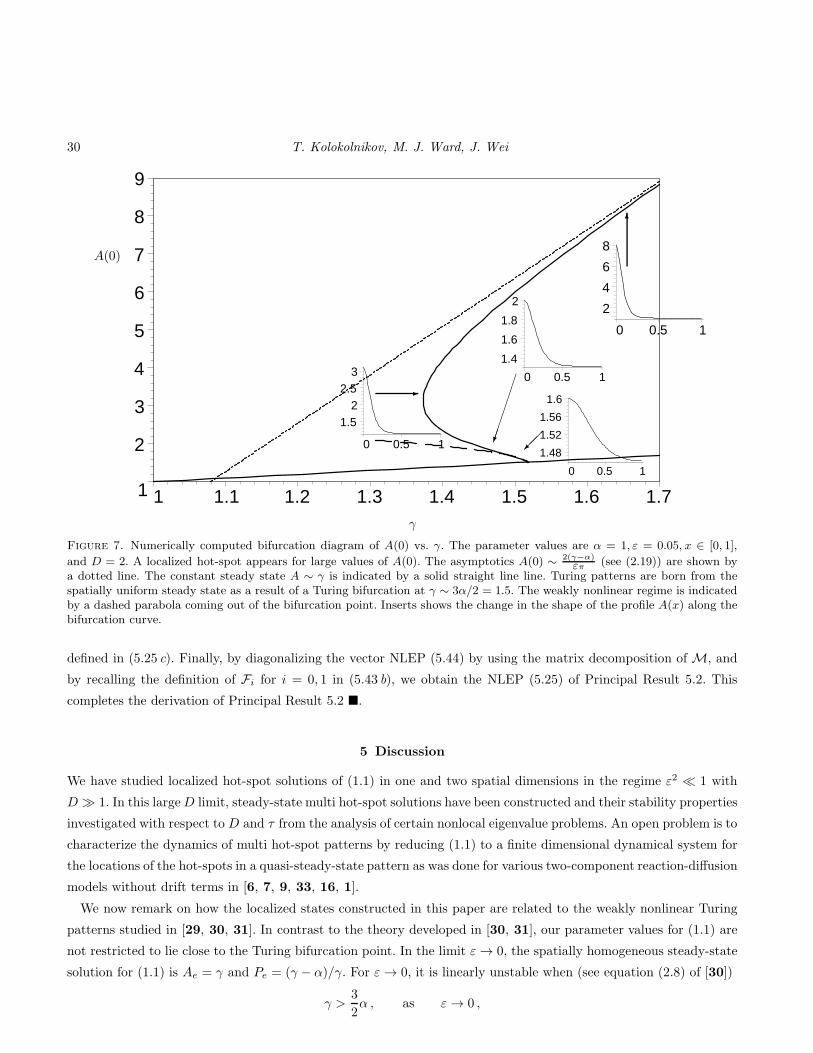
30 T. Kolokolnikov, M. J. Ward, J. Wei
1
2
3
4
5
6
7
8
9
1 1.1 1.2 1.3 1.4 1.5 1.6 1.7
2
4
6
8
0 0.5 1
1.4
1.6
1.8
2
0 0.5 1
1.48
1.52
1.56
1.6
0 0.5 1
1.52
2.53
0 0.5 1
-
6
γ
A(0)
Figure 7. Numerically computed bifurcation diagram of A(0) vs. γ. The parameter values are α = 1, ε = 0.05, x ∈ [0, 1],
and D = 2. A localized hot-spot appears for large values of A(0). The asymptotics A(0) ∼ 2(γ−α)επ (see (2.19)) are shown by
a dotted line. The constant steady state A ∼ γ is indicated by a solid straight line line. Turing patterns are born from thespatially uniform steady state as a result of a Turing bifurcation at γ ∼ 3α/2 = 1.5. The weakly nonlinear regime is indicatedby a dashed parabola coming out of the bifurcation point. Inserts shows the change in the shape of the profile A(x) along thebifurcation curve.
defined in (5.25 c). Finally, by diagonalizing the vector NLEP (5.44) by using the matrix decomposition of M, and
by recalling the definition of Fi for i = 0, 1 in (5.43 b), we obtain the NLEP (5.25) of Principal Result 5.2. This
completes the derivation of Principal Result 5.2 .
5 Discussion
We have studied localized hot-spot solutions of (1.1) in one and two spatial dimensions in the regime ε2 ≪ 1 with
D ≫ 1. In this largeD limit, steady-state multi hot-spot solutions have been constructed and their stability properties
investigated with respect to D and τ from the analysis of certain nonlocal eigenvalue problems. An open problem is to
characterize the dynamics of multi hot-spot patterns by reducing (1.1) to a finite dimensional dynamical system for
the locations of the hot-spots in a quasi-steady-state pattern as was done for various two-component reaction-diffusion
models without drift terms in [6, 7, 9, 33, 16, 1].
We now remark on how the localized states constructed in this paper are related to the weakly nonlinear Turing
patterns studied in [29, 30, 31]. In contrast to the theory developed in [30, 31], our parameter values for (1.1) are
not restricted to lie close to the Turing bifurcation point. In the limit ε→ 0, the spatially homogeneous steady-state
solution for (1.1) is Ae = γ and Pe = (γ − α)/γ. For ε→ 0, it is linearly unstable when (see equation (2.8) of [30])
γ >3
2α , as ε→ 0 ,
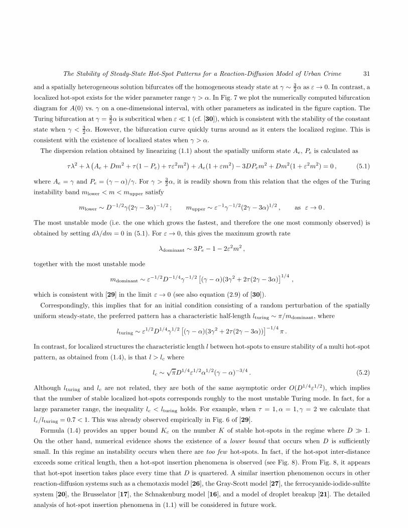
The Stability of Steady-State Hot-Spot Patterns for a Reaction-Diffusion Model of Urban Crime 31
and a spatially heterogeneous solution bifurcates off the homogeneous steady state at γ ∼ 32α as ε→ 0. In contrast, a
localized hot-spot exists for the wider parameter range γ > α. In Fig. 7 we plot the numerically computed bifurcation
diagram for A(0) vs. γ on a one-dimensional interval, with other parameters as indicated in the figure caption. The
Turing bifurcation at γ = 32α is subcritical when ε≪ 1 (cf. [30]), which is consistent with the stability of the constant
state when γ < 32α. However, the bifurcation curve quickly turns around as it enters the localized regime. This is
consistent with the existence of localized states when γ > α.
The dispersion relation obtained by linearizing (1.1) about the spatially uniform state Ae, Pe is calculated as
τλ2 + λ(
Ae +Dm2 + τ(1 − Pe) + τε2m2)
+Ae(1 + εm2)− 3DPem2 +Dm2(1 + ε2m2) = 0 , (5.1)
where Ae = γ and Pe = (γ − α)/γ. For γ > 32α, it is readily shown from this relation that the edges of the Turing
instability band mlower < m < mupper satisfy
mlower ∼ D−1/2γ(2γ − 3α)−1/2 ; mupper ∼ ε−1γ−1/2(2γ − 3α)1/2 , as ε→ 0 .
The most unstable mode (i.e. the one which grows the fastest, and therefore the one most commonly observed) is
obtained by setting dλ/dm = 0 in (5.1). For ε→ 0, this gives the maximum growth rate
λdominant ∼ 3Pe − 1− 2ε2m2 ,
together with the most unstable mode
mdominant ∼ ε−1/2D−1/4γ−1/2[
(γ − α)(3γ2 + 2τ(2γ − 3α)]1/4
,
which is consistent with [29] in the limit ε→ 0 (see also equation (2.9) of [30]).
Correspondingly, this implies that for an initial condition consisting of a random perturbation of the spatially
uniform steady-state, the preferred pattern has a characteristic half-length lturing ∼ π/mdominant, where
lturing ∼ ε1/2D1/4γ1/2[
(γ − α)(3γ2 + 2τ(2γ − 3α))]−1/4
π .
In contrast, for localized structures the characteristic length l between hot-spots to ensure stability of a multi hot-spot
pattern, as obtained from (1.4), is that l > lc where
lc ∼√πD1/4ε1/2α1/2(γ − α)−3/4 . (5.2)
Although lturing and lc are not related, they are both of the same asymptotic order O(D1/4ε1/2), which implies
that the number of stable localized hot-spots corresponds roughly to the most unstable Turing mode. In fact, for a
large parameter range, the inequality lc < lturing holds. For example, when τ = 1, α = 1, γ = 2 we calculate that
lc/lturing = 0.7 < 1. This was already observed empirically in Fig. 6 of [29].
Formula (1.4) provides an upper bound Kc on the number K of stable hot-spots in the regime where D ≫ 1.
On the other hand, numerical evidence shows the existence of a lower bound that occurs when D is sufficiently
small. In this regime an instability occurs when there are too few hot-spots. In fact, if the hot-spot inter-distance
exceeds some critical length, then a hot-spot insertion phenomena is observed (see Fig. 8). From Fig. 8, it appears
that hot-spot insertion takes place every time that D is quartered. A similar insertion phenomenon occurs in other
reaction-diffusion systems such as a chemotaxis model [26], the Gray-Scott model [27], the ferrocyanide-iodide-sulfite
system [20], the Brusselator [17], the Schnakenburg model [16], and a model of droplet breakup [21]. The detailed
analysis of hot-spot insertion phenomena in (1.1) will be considered in future work.
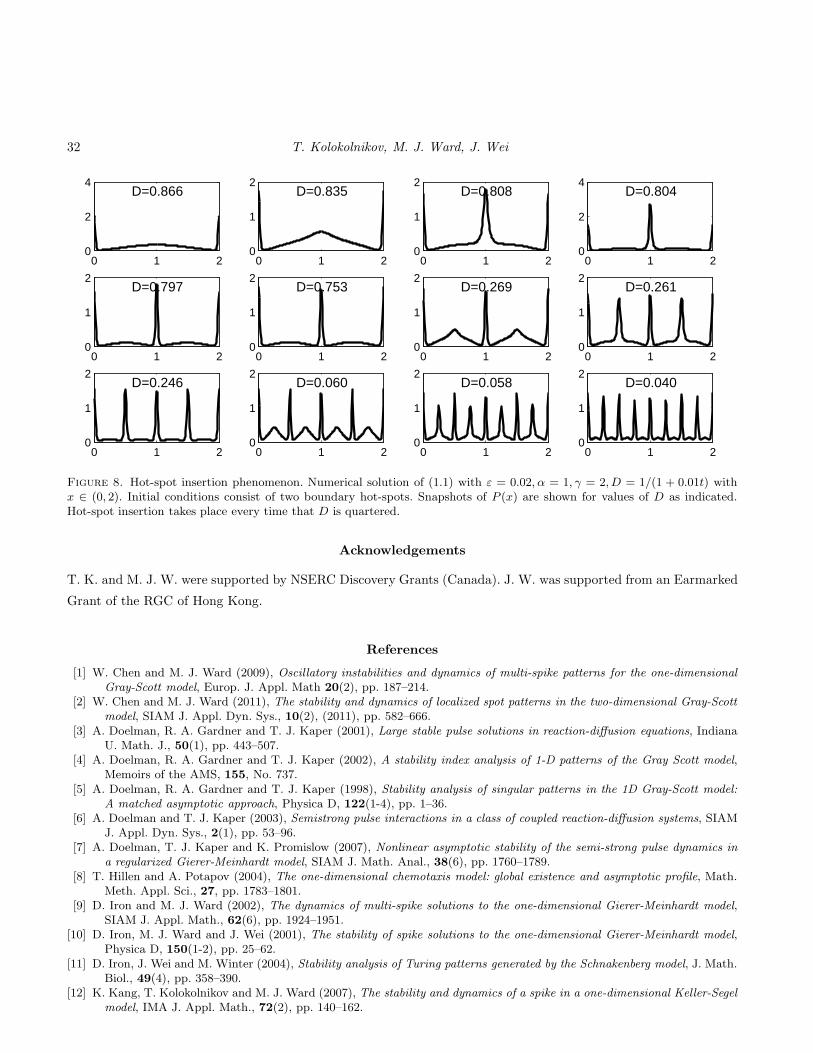
32 T. Kolokolnikov, M. J. Ward, J. Wei
0 1 20
2
4D=0.866
0 1 20
1
2D=0.835
0 1 20
1
2D=0.808
0 1 20
2
4D=0.804
0 1 20
1
2D=0.797
0 1 20
1
2D=0.753
0 1 20
1
2D=0.269
0 1 20
1
2D=0.261
0 1 20
1
2D=0.246
0 1 20
1
2D=0.060
0 1 20
1
2D=0.058
0 1 20
1
2D=0.040
Figure 8. Hot-spot insertion phenomenon. Numerical solution of (1.1) with ε = 0.02, α = 1, γ = 2, D = 1/(1 + 0.01t) withx ∈ (0, 2). Initial conditions consist of two boundary hot-spots. Snapshots of P (x) are shown for values of D as indicated.Hot-spot insertion takes place every time that D is quartered.
Acknowledgements
T. K. and M. J. W. were supported by NSERC Discovery Grants (Canada). J. W. was supported from an Earmarked
Grant of the RGC of Hong Kong.
References
[1] W. Chen and M. J. Ward (2009), Oscillatory instabilities and dynamics of multi-spike patterns for the one-dimensional
Gray-Scott model, Europ. J. Appl. Math 20(2), pp. 187–214.[2] W. Chen and M. J. Ward (2011), The stability and dynamics of localized spot patterns in the two-dimensional Gray-Scott
model, SIAM J. Appl. Dyn. Sys., 10(2), (2011), pp. 582–666.[3] A. Doelman, R. A. Gardner and T. J. Kaper (2001), Large stable pulse solutions in reaction-diffusion equations, Indiana
U. Math. J., 50(1), pp. 443–507.[4] A. Doelman, R. A. Gardner and T. J. Kaper (2002), A stability index analysis of 1-D patterns of the Gray Scott model,
Memoirs of the AMS, 155, No. 737.[5] A. Doelman, R. A. Gardner and T. J. Kaper (1998), Stability analysis of singular patterns in the 1D Gray-Scott model:
A matched asymptotic approach, Physica D, 122(1-4), pp. 1–36.[6] A. Doelman and T. J. Kaper (2003), Semistrong pulse interactions in a class of coupled reaction-diffusion systems, SIAM
J. Appl. Dyn. Sys., 2(1), pp. 53–96.[7] A. Doelman, T. J. Kaper and K. Promislow (2007), Nonlinear asymptotic stability of the semi-strong pulse dynamics in
a regularized Gierer-Meinhardt model, SIAM J. Math. Anal., 38(6), pp. 1760–1789.[8] T. Hillen and A. Potapov (2004), The one-dimensional chemotaxis model: global existence and asymptotic profile, Math.
Meth. Appl. Sci., 27, pp. 1783–1801.[9] D. Iron and M. J. Ward (2002), The dynamics of multi-spike solutions to the one-dimensional Gierer-Meinhardt model,
SIAM J. Appl. Math., 62(6), pp. 1924–1951.[10] D. Iron, M. J. Ward and J. Wei (2001), The stability of spike solutions to the one-dimensional Gierer-Meinhardt model,
Physica D, 150(1-2), pp. 25–62.[11] D. Iron, J. Wei and M. Winter (2004), Stability analysis of Turing patterns generated by the Schnakenberg model, J. Math.
Biol., 49(4), pp. 358–390.[12] K. Kang, T. Kolokolnikov and M. J. Ward (2007), The stability and dynamics of a spike in a one-dimensional Keller-Segel
model, IMA J. Appl. Math., 72(2), pp. 140–162.
The Stability of Steady-State Hot-Spot Patterns for a Reaction-Diffusion Model of Urban Crime 33
[13] T. Kolokolnikov and M. J. Ward (2003), Reduced-wave Green’s functions and their effect on the dynamics of a spike for
the Gierer-Meinhardt model, Europ. J. Appl. Math., 14(5), pp. 513–545.[14] T. Kolokolnikov and M. J. Ward (2004), Bifurcation of spike equilibria in a near shadow reaction-diffusion System,
DCDS-B, 4(4), pp. 1033–1064.[15] T. Kolokolnikov, M. J. Ward and J. Wei (2005), The existence and stability of spike equilibria in the one-dimensional
Gray-Scott model: The low feed-rate regime, Studies in Appl. Math., 115(1), pp. 21–71.[16] T. Kolokolnikov, M. J. Ward and J. Wei (2009), Spot self-replication and dynamics for the Schnakenburg model in a
two-dimensional domain, J. Nonlinear Sci., 19(1), pp. 1–56.[17] T. Kolokolnikov, M. J. Ward, and J. Wei (2007), Self-replication of mesa patterns in reaction-diffusion models, Physica
D, 236(2), pp. 104–122.[18] T. Koloklonikov, M. J. Ward and J. Wei (2006), Slow translational instabilities of spike patterns in the one-dimensional
Gray-Scott model, Interfaces and Free Boundaries, 8(2), pp. 185–222.[19] T. Kolokolnikov and J. Wei (2011), Stability of spiky solutions in a competition model with cross-diffusion, SIAM J. Appl.
Math. 71, pp. 1428–1457.[20] K. J. Lee and H. L. Swinney (1995), Lamellar structures and self-replicating spots in a reaction-diffusion systems, Phys.
Rev. E., 51(3), pp. 1899–1915.[21] W. Liu, A. L. Bertozzi, and T. Kolokolnikov (2012), Diffuse interface surface tension models in an expanding flow, Comm.
Math. Sci., 10(1), pp. 387–418.[22] R. McKay and T. Kolokolnikov (2012), Stability transitions and dynamics of localized patterns near the shadow limit of
reaction-diffusion systems, to appear, DCDS-B.[23] C. B. Muratov and V. V. Osipov (2002), Stability of static spike autosolitons in the Gray-Scott model, SIAM J. Appl.
Math., 62(5), pp. 1463–1487.[24] C. B. Muratov and V. V. Osipov (2000), Static spike autosolitons in the Gray-Scott model, J. Phys. A: Math Gen., 33,
pp. 8893–8916.[25] Y. Nishiura (2002), Far-from equilibrium dynamics, translations of mathematical monographs, Vol. 209, AMS Publications,
Providence, Rhode Island.[26] K. Painter and T. Hillen (2011), Spatio-temporal chaos in a chemotaxis Model, Physica D, 240, pp. 363–375.[27] J. E. Pearson (1993), Complex Patterns in a Simple System, Science, 216, pp. 189–192.[28] A. Potapov and T. Hillen (2005), Metastability in chemotaxis models, J. Dynam. Diff. Eq., 17(2) pp. 293-330.[29] M. B. Short, M. R. D’Orsogna, V. B. Pasour, G. E. Tita, P. J. Brantingham, A. L. Bertozzi and L. B. Chayes (2008), A
statistical model of criminal behavior, Math. Models. Meth. Appl. Sci., 18, Suppl. pp. 1249–1267.[30] M. B. Short, A. L. Bertozzi and P. J. Brantingham (2010), Nonlinear patterns in urban crime - hotpsots, bifurcations,
and suppression, SIAM J. Appl. Dyn. Sys., 9(2), pp. 462–483.[31] M. B. Short, P. J. Brantingham, A. L. Bertozzi and G. E. Tita (2010), Dissipation and displacement of hotpsots in
reaction-diffusion models of crime, Proc. Nat. Acad. Sci. 107(9) pp. 3961-3965.[32] B. Sleeman, M. J. Ward and J. Wei (2005), The existence and stability of spike patterns in a chemotaxis model, SIAM J.
Appl. Math., 65(3), pp. 790–817.[33] W. Sun, M. J. Ward and R. Russell (2005), The slow dynamics of two-spike solutions for the Gray-Scott and Gierer-
Meinhardt systems: competition and oscillatory instabilities, SIAM J. Appl. Dyn. Syst., 4(4), pp. 904–953.[34] H. Van der Ploeg and A. Doelman (2005), Stability of spatially periodic pulse patterns in a class of singularly perturbed
reaction-diffusion equations, Indiana Univ. Math. J., 54(5), p. 1219-1301.[35] M. J. Ward and J. Wei (2003), Hopf bifurcations and oscillatory instabilities of spike solutions for the one-dimensional
Gierer-Meinhardt model, J. Nonlinear Sci., 13(2), pp. 209–264.[36] M. J. Ward and J. Wei (2002), The existence and stability of asymmetric spike patterns in the Schnakenburg model,
Studies in Appl. Math., 109(3), pp. 229–264.[37] M. J. Ward and J. Wei (2002), Asymmetric spike patterns for the one-dimensional Gierer-Meinhardt model: equilibria
and stability, Europ. J. Appl. Math., 13(3), (2002), pp. 283–320.[38] M. J. Ward and J. Wei (2003), Hopf bifurcation of spike solutions for the shadow Gierer-Meinhardt model, Europ. J. Appl.
Math., 14(6), pp. 677–711.[39] J. Wei and M. Winter (2001), Spikes for the two-dimensional Gierer-Meinhardt system: the weak coupling case, J. Nonlinear
Sci., 11(6), pp. 415–458.[40] J. Wei and M. Winter (2002), Spikes for the two-dimensional Gierer-Meinhardt system: the strong coupling case, J. Diff.
Eq., 178, pp. 478–518.[41] J. Wei and M. Winter (2003), Existence and stability of multiple spot solutions for the Gray-Scott model in R
2, PhysicaD., 176(3-4), pp. 147-180.
[42] J. Wei and M. Winter (2008), Stationary multiple spots for reaction-diffusion systems, J. Math. Biol., 57(1), pp. 53–89.[43] J. Wei and M. Winter (2004), Existence and stability analysis of asymmetric patterns for the Gierer-Meinhardt system,
J. Math. Pures Appl. (9), 83(4), pp. 433-476.

34 T. Kolokolnikov, M. J. Ward, J. Wei
[44] J. Wei and M. Winter (2003), Asymmetric spotty patterns for the Gray-Scott model in R2, Studies in Appl. Math.,
110(1), pp. 63–102.[45] J. Wei and L. Zhang (1998), On a nonlocal eigenvalue problem, Ann. Sc. Norm. Sup. Pisa C1. Sci. pp. 41–62.[46] J. Wei (2008), Existence and stability of spikes for the Gierer-Meinhardt system, book chapter in Handbook of Differential
Equations, Stationary Partial Differential Equations, Vol. 5 (M. Chipot ed.), Elsevier, pp. 489–581.