Embed Size (px)
Citation preview

RIGHT:
URL:
CITATION:
AUTHOR(S):
ISSUE DATE:
TITLE:
Stability of Steady States and Steady-StateLimit of Elastoplastic Trusses under Quasi-Static Cyclic Loading( Dissertation_全文 )
Araki, Yoshikazu
Araki, Yoshikazu. Stability of Steady States and Steady-State Limit of Elastoplastic Trussesunder Quasi-Static Cyclic Loading. 京都大学, 1998, 博士(工学)
1998-03-23
https://doi.org/10.11501/3135459
STABILITY OF STEADY STATES AND
STEADY~STATE LIMIT OF
ELASTOPLASTICTRUSSESUNDER
QUASI-STATICCYCLid LOApING',t;
i
.........'.
I
1101
,.
;..:.'
By
i"i., /-
': ,,,,-'
.~ ;
;-\.
"" r"/ ~~. - . ',;.' :',
'. '
~ , ...
.....,..,.,.
{,
..,"
".",
• ·f~
.,'-;
; ...
...~ 'f
"'""':..',-1 ..'-'.
. ;
STABILITY OF STEADY STATES AND
STEADY-STATE LIMIT OF
ELASTOPLASTIC TRUSSES UNDER
QUASI-STATIC CYCLIC LOADING
By
Yoshikazli Araki
December 1997


.,.•..•..."l:.CI.;

Acknowledgments
I would especially like to acknowledge Professor Koji Uetani. In the development of this
work, I have benefited from his guidance of interesting research topics, and from advises,
suggestions, and discussions. The topic of "steady-state limit of elastoplastic structures"
was originally developed by Professor Koji Uetani for cantilever beam-columns. And he has
guided me the topic throughout my graduate study. His energetic attitude towards research
has been encouraged me to do further research.
I am grateful of Prof. B. Tsuji and Prof. H. Kunieda for reading this manuscript. I
express sincere appreciation to Dr. 1. Takewaki and Dr. M. Ohsaki for providing valuable
advises on my research and for reading a part of this thesis. I thank to Mr. T. Masui and
Mr. H. Tagawa for their positive comments. I wish to acknowledge Dr. T. Nakamura for
his valuable suggestions at the early stage of this work. Thanks are due to Miss. T. Yorifuji
who supported a part of numerical analyses.
It has been a pleasure to work with the students in master and undergraduate courses.
Discussions with them have been stimulated me to find and remember the problems that
would have been missed without their honest comments. I acknowledge the financial support
provided by JSPS Research Fellowships for Young Scientists for these two years. Finally, I
am truly grateful of all of the help and encouragement I have received in the development
of this work.
Finally, I am greatly indebted to my mother Natsue Araki for her tireless support and
patience.
v


Contents
1 Introduction 1
1.1 BACKGROUND 1
1.2 SCOPE ...... 4
1.3 LIMITATIONS 6
1.4 TERMINOLOGY. 6
2 Steady-State Limit for Elastic Shakedown Region 11
2.1 INTRODUCTION ••• 4 •• 11
2.2 GOVERNING EQUATIONS. 14
2.2.1 Analytical Model 14
2.2.2 Cyclic Responses 16
2.3 FUNDAMENTAL CONCEPTS 17
2.3.1 Loading Conditions . 17
2.3.2 Hypotheses 18
2.3.3 Outline 19
2.4 FORMULATION 19
2.4.1 Incremental Relations for Variation of Steady State 19
2.4.2 Rate Forms of Governing Equations . . . . . . . . . 20
2.4.3 Consistent Set of Stress Rate-Strain Rate Relations 22
2.4.4 Termination Conditions for Incremental Step. 23
2.4.5 Steady-State Limit Condition 24
2.5 NUMERICAL EXAMPLES a a a .. 24
2.5.1 Steady-State Limit Analysis 24
2.5.2 Response Analysis 27
2.6 CONCLUSIONS ..... 29
Vll
3 Steady-State Limit for Plastic Shakedown Region 39
3.1 INTRODUCTION 39
3.2 GOVERNING EQUATIONS. 41
3.2.1 Analytical Model . . 41
3.2.2 Loading Conditions. 43
3.2.3 Steady-State Responses in Stress-Strain Plane 43
3.3 PRELIMINARY CONSIDERATIONS 45
3.3.1 Fundamental Concepts for Steady-State Limit Theory in Elastic Shake-
down Region 45
3.3.2 Numerical Study on Strain Reversals 46
3.3.3 General Consideration on Strain Reversals 48
3.3.4 Fundamental Concepts for Steady-State Limit Theory in Plastic Shake-
down Region 48
3.4 FORMULATION.. 49
3.4.1 Incremental Relations for Variation of Steady State 49
3.4.2 Rate Forms of Governing Equations . . . . . . . . . 50
3.4.3 Consistent Set of Stress Rate-Strain Rate Relations 53
3.4.4 Termination Conditions for Incremental Steps 53
3.4.5 Examination of Strain Reversals . 54
3.4.6 Steady-State Limit Condition 56
3.5 NUMERICAL EXAMPLES . . . . 57
3.5.1 Steady-state limit Analysis. 57
3.5.2 Response Analysis 59
3.6 CONCLUSIONS .... . 60
4 Stability of Steady States and Steady-State Limit 69
4.1 INTRODUCTION 69
4.2 GOVERNING EQUATIONS. 71
4.2.1 Analytical Models. . 71
4.2.2 Loading Conditions. 73
4.3 STEADY STATES. . . . . 73
4.3.1 Outline of Formulation 73
4.3.2 Tangent Stiffness Equations 75
4.3.3 Termination Conditions for Incremental Steps 76
Vlll
4.3.4 Stress-Strain Responses ....... 77
4.4 DEVIATION FROM STEADY STATES 77
4.4.1 Outline of Formulation ...... 77
4.4.2 Rate Relations at Arbitrary Instants 79
4.4.3 Recurrence Relations between Consecutive Periodic Instants 80
4.4.4 Stress-Strain Responses ... 81
4.5 STABILITY OF STEADY STATES 82
4.5.1 Definition of Stability. 82
4.5.2 Stability Criterion 82
4.6 STEADY-STATE LIMIT. 84
4.6.1 Outline of Formulation 84
4.6.2 Rate Relations for Variation of Steady States 84
4.6.3 Consistent Set of Stress-Strain Responses . . . 85
4.6.4 Termination Conditions for Incremental Steps 85
4.6.5 Steady-State Limit Condition 86
4.7 NUMERICAL EXAMPLES 87
4.8 CONCLUSIONS ....... 91
5 Concluding Remarks 101
IX
Chapter 1
Introduction
1.1 BACKGROUND
In current and common seismic design of building structures, the buildings are designed
so that the following requirements are satisfied: (1) In moderate earthquakes, which occur
frequently, no plastic deformation takes place; and (2) In strong earthquakes, which happen
rarely, plastifications of their structural elements are allowed but total collapse should be
avoided. Namely, plastic deformations are allowed in case of strong earthquakes. In addition
to this fact, there is a tendency to use deliberately the energy absorption due to the plastic
deformations in order to control the displacements and accelerations caused by earthquakes.
To clarify the fundamental properties of the structural response with plastic deformations,
extensive research has been done on the elastoplastic response of structures subjected to
quasi-static loads (see, e.g. [1, 2, 3, 4, 5, 6]). According to whether the loading condition is
monotonic or cyclic, the research is classified into eight categories shown in Table 1.1. The
Table 1.1: Classification of elastoplastic analysis.
Monotonic Loading Cyclic Loading
Limit Analysis
Plastic Buckling Theory
Tracing All Loading History Tracing All Loading History
Shakedown Theory
Symmetry Limit Theory,
Steady-State Limit Theory
Stability of Equilibrium States Stability of Steady States
1
main objectives of the research are: (1) to clarify how structures behave under the quasi
static loads; and (2) to find the critical loading condition beyond which unstable responses
occur.
The plastic buckling and the plastic collapse have been mainly considered in the research.
In addition to these types of instability, it is known that, plastic deformations of struc
tures under cyclic loads may accumulate proportionally or exponentially with respect to the
number of the cycles. The accumulation may lead to the degradation of load capacity and
stiffness. Obviously, no stable energy dissipation can be expected in this case. This phenom
ena is considered to be a type of instability and is the main subject of this thesis. By the
way, although fractures are frequently observed in strong earthquakes [7, 8], our discussion
is limited to the case where neither ductile nor brittle cracking occurs.
Under both monotonic and cyclic loads, a direct but elaborating approaches for investigat
ing the elastoplastic response is to trace the all loading history of structures. Experimental,
analytical, and numerical methods are available for this purpose. By tracing the all loading
history, we can observe the whole process of the deformations and find the loading condi
tions below which structures behave in a stable manner. Nonetheless, generally, analytical
methods can be applied only to very simple models. Experimental and numerical approaches
require a number of parametric analyses to bound the stable response. Moreover, it is very
difficult to derive the theoretical condition similar to that for the Euler buckling load from
the results of the parametric analyses.
For the stability of elastoplastic structures subjected to monotonic loads, theoretical foun
dation seems to be established. As a theory of stability, the limit analysis [9] is well known
and widely used in structural design. In the limit analysis, both collapse loads and col
lapse modes are obtained based on the upper bound or the lower bound theorem. The limit
analysis is originally developed for the structures with perfectly plastic material. And the
effect of geometrical nonlinearity is completely neglected in the theory of the limit analysis.
Another well-known theory on stability is the plastic buckling theory [10]. Plastic buckling
is predicted as the fist bifurcation or limit points of equilibrium paths, which represents the
variation of equilibrium states under the monotonic loads. In addition, based on the defini
tion of stability due to Liapunov [11], a general criterion on the stability of an equilibrium
state was derived by Hill [12] for elastoplastic structures.
On the other hand, the stability of elastoplastic structures under quasi-static cyclic loads
appears to remain as research subjects. As a theoretical approach, the shakedown theory [13]
is well known. In the shakedown theory, we can find the domain of the cyclic loads within
2

which a structure converges to a shakedown response regardless of loading histories based
on the upper bound or lower bound theorem. Similar to the limit analysis, the classical
shakedown theory was developed for the structures composed of perfectly plastic materials
without taking into account geometrical nonlinearity. Several papers extended in recent
years the shakedown theory taking the geometrical nonlinearity into consideration, (see e.g.
[14, 15, 16, 17]). But the path-independent shakedown theories have inherent difficulties
when geometrical nonlinearity plays crucial role. This is because the responses are path
dependent in this case [1].
In such situations, Uetani and Nakamura [18, 19, 20] proposed the symmetry limit theory
and the steady-state limit theory for cantilever beam-columns subjected to cyclic bending in
the presence of a compressive axial force. With these two theories, though under a specified
loading history, we can find the limit that bounds convergence and divergence of plastic
deformations as a mathematical critical point even if geometrical nonlinearity has strong
effect on structural responses. In the two theories, a steady state and variation of the steady
state generated under the idealized cyclic loading with continuously increasing amplitude are
regarded as a point and a continuous path, respectively. In analogy with an equilibrium state
and an equilibrium path, the continuous path is called steady-state path. The symmetry
limit and the steady-state limit are predicted as the first branching and limit points of the
steady-state path, respectively.
For a few classes of structures, the symmetry limit theory and the steady-state limit
theory have been applied. Severe degradation of load capacity and stiffness were observed
if the deflection amplitude was in excess of the symmetry limit or the steady-state limit
[19, 21, 20]. In those studies, however, only the simple structures, e.g. a cantilever beam
column or a unit frame, were treated for which analytical solutions can be derived. Hence,
to investigate the limit states of more complex and practical structures, which generally do
not have symmetry limits if they do not have symmetric shapes, it is necessary to establish
a method for predicting the steady-state limit using appropriate finite element methods. In
addition, it is desirable from theoretical view, by analogy with the stability of equilibrium
state, to introduce the concept of stability of steady states or closed orbits and to characterize
the steady-state limit as the steady state at which the stability of the steady states is lost
[19, 20]. This concept of the stability of closed orbits is well known for the elastic structures
subjected to dynamic loads (see, for instance [22, 23, 24]). But, to the best of author's
knowledge, no clear stability criterion has been given for elastoplastic structures subjected
to dynamic or quasi-static cyclic loads.
3
1.2 SCOPE
This research has two purposes. One is to generalize the steady-state limit theory, originally
developed for cantilever beam-columns; so as to find the steady-state limits of elastoplastic
trusses subjected to cyclic, quasi-static and proportional loading in the presence of constant
loads. The other is to introduce the concept of stability of steady states into the quasi-static
problem of elastoplastic structures under cyclic loads.
This research is part of the project that aims to develop the theories and methods for
predicting the critical loading conditions that bound convergence and divergence of defor
mations of elastoplastic structures with arbitrary shapes and materials. For this purpose,
appropriate discretization schemes, such as finite element methods; seem to be promising.
We treat only trusses in this research for simplicity. But the theories presented in this thesis
can be easily extended to the elastoplastic structures with arbitrary shapes whose behavior
is described by uni-axial stress-strain relations. In fact, one of the present methods has been
successfully applied to moment-resisting frames with a fiber element [25]. In addition, anoth
er theory presented in this thesis is expected to be directly applicable to three dimensional
continua with almost no restriction.
Toward the ends stated above, the specific subjects of this study are described as follows:
1. To formulate incremental relations for the variation of the steady states of trusses with
respect to the variation of the amplitude of cyclic loading.
2. To relax and exclude the basic assumption on strain reversals employed in the previous
steady-state limit theory for cantilever beam-columns.
3. To derive the stability criterion of steady states and to characterize the steady-state
limit as the critical steady state at which the stability is lost.
The relations between these subjects and the composition of this thesis are written in the
following paragraphs. All chapters are written to be as self-consistent as possible. Through
out this thesis, validity of the hypothesis and the results of the proposed methods are shown
in numerical examples.
In chapter 2 a method is presented for finding the steady-state limits that bound conver
gence to elastic shakedown and divergence of plastic deformations. The method is a simple
extension of the steady-state limit theory for cantilever beam-columns. But a chapter is
assigned to this method because it provide the backbone of the methods presented in the
later chapters. In the present method, a steady state is uniquely described by the state
4

variables at load reversals by assuming that strain reversals in steady states occur only at
load reversals. By differentiating all the state variables representing a steady state and by
using the Taylor series expansion, new incremental relations are formulated for tracing a
steady-state path, which represents variation of a steady state under the idealized cyclic
loading program with continuously increasing amplitude. The steady-state limit is found as
the first limit point of the steady-state path.
Chapter 3 presents a theory and method for finding the steady-state limit that bounds
divergence of plastic deformations and convergence to plastic shakedown. When plastic
shakedown occurs, strain reversals may take place not only at load reversals but also at the
yielding of the elements exhibiting the plastic shakedown. The previous approach cannot be
applied to such cases because the assumption on strain reversals in the previous method is
not valid in such a case. This difficulty is overcome by relaxing the assumption so that the
strain reversals due to the yielding is taken into account. Based on the relaxed assumption, a
steady state is described by the state variables not only at load reversals but also at yielding
points of the elements exhibiting plastic shakedown. This is the key extension from the
methods presented in the previous chapter. Once a steady state is represented by a set of
equilibrium states, similar to the previous method, incremental relations are formulated by
differentiating the state variables, steady-state path is traced incrementally, and the steady
state limit is found as the first limit point of the steady-state path.
In chapter 4, an alternative method is presented for tracing the steady-state paths, and
a theory is developed for finding the steady-state limit as the critical steady state at which
loss of the stability of steady states occurs. In this method, first, a steady state is expressed
by discretizing its equilibrium path with respect to an equilibrium path parameter. Second,
deviation from the steady state due to the change of the amplitude of cyclic loading is
expressed using the recurrence equation that relates two consecutive periodic instants. The
recurrence equation is formulated in terms of the plastic strain increments with respect to the
change of the amplitude of cyclic loads. Then the stability of the steady state is rigorously
defined and the stability criterion is given in terms of the eigenvalue of the coefficient matrix
in the recurrence equation. The steady-state path is traced using the recurrence equation,
and the steady-state limit is found as the critical steady state at which the stability of steady
states is lost.
Finally, concluding remarks are made in section 5. Advantages and drawbacks are written
for the methods proposed in this thesis. Subjects of future research are summarized.
5
1.3 LIMITATIONS
The assumptions and limitations made in this research are listed below:
• Analytical models are pin-jointed space trusses.
• Buckling of the element is ruled out. But buckling of a global type is taken into account.
• Only quasi-static loads are applied. In other words, dynamic effects are neglected.
• For both constant and cyclic loads, only proportional loading is considered.
• Stresses and strains are measured using the Total Lagrangian formulation.
• Assumptions of large displacements-small strains are employed.
• As a uni-axial constitutive law, bi-linear kinematic hardening rule is employed. Thermal
effect is neglected. Cyclic hardening and cyclic softening is neglected.
• Neither brittle nor ductile cracking is considered.
1.4 TERMINOLOGY
The terminology used in this paper is briefly summarized. More rigorous definition of these
terms are given in the following chapters.
• Steady State: When elastoplastic structures are subjected to quasi-static cyclic loads,
its response may converge to a cyclic response. The cyclic response is called a steady
state.
• Elastic Shakedown, Classical Shakedown, Shakedown: A cyclic and fully elastic struc
tural response after some histories of plastic deformations.
• Plastic Shakedown, Alternating Plasticity: The steady state in which plastic deforma
tions are included.
• Cyclic Instability, Incremental Collapse, Ratchetting: The state in which deformation
grows proportionally or exponentially with respect to the number of the cycles.
• Idealized Cyclic Loading Program: The loading program where the amplitude of the load
factor of proportional loads is continuously increased. At each level of the amplitude,
the loading cycle is repeated as many times as necessary for convergence.
• Steady-State Path: Under the idealized cyclic loading program, variation of a steady
state can be regarded as a path. This path is called a steady-state path.
• Symmetric Steady State, Asymmetric Steady State: A steady state is called a symmetric
steady state if a pair of the deflected configurations at load reversals is symmetric with
6
respect to the initial symmetric axis. Otherwise, the steady sate is called asymmetric
steady state.
• Symmetry Limit: The symmetry limit is the critical steady state at which transition
from the symmetric steady state to the asymmetric steady state can occur under the
idealized cyclic loading program.
• Steady-State Limit: The steady-state limit is the critical steady state beyond which
structures will no longer exhibit any convergent behavior under the idealized cyclic
loading program.
• Stability of Steady States: A steady state is said to be stable if a small change in the
amplitude of cyclic loading leads to a small change in the responses. Otherwise, the
steady state is said to be unstable.
7
References
[1] J. A. Konig. Shakedown of Elastic-Plastic Structures. Elsevier, Amsterdam, 1987.
[2] W. F. Chen and D. J. Han. Plasticity for Structural Engineering. Springer-Verlag, New
York, 1988.
I3] P. Z. Bazant and L. Cedolin. Stability of Structures. Oxford University Press, New
York, 1991.
[4] AU. Unstable Behavior and Limit State of Structures, volume 1. Maruzen, 1994. (in
Japanese).
[5] AU. Recommendations for Stability Design of Steel Structures. Maruzen, 1996. (in
Japanese) .
[6] AU. Collapse Analysis of Structures, volume 1. Maruzen, 1997. (in Japanese).
[7] V. V. Bertero, J. C. Anderson, and H. Krawinkler. Performance of steel building struc
ture during the northlidge earthquake. Technical Report UCB/EERC-94/09, Earth~
quake Research Center, 1994.
[8] Building Research Institute. A survey report for building damages due to the 1995
Hyogo-ken Nanbu earthquake. Building Research Institute, Ministry of Construction,
1996.
[9] D. C. Drucker, W. Prager, and H. J. Greenberg. Extended limit design theorems for
continuous media. Quartry of Applied Mathematics, 9:381-389, 1952.
[10] F. R. Shanley. Inelastic column theory. Journal of Aeronautical Sciences, 14:261-268,
1947.
[11] A. M. Liapunov. The General Problem of the Stability of Motion. Taylor & Francis,
London, 1992. Translated and edited by A. T. Fuller.
[12] R. Hill. A general theory of uniqueness and stability in elastic-plastic solids. Journal
of the Mechanics and Physics of Solids, 6:236-249, 1958.
[13] W. T. Koiter. General theorems for elastic-plastic structures. In J. N. Sneddon and
R. Hill, editors, Progress in Solid Mechanics, volume 1, pages 167-221, North Holland,
Amsterdam, 1960.
[14] G. Maier. A shakedown matrix theory allowing for workhardening and second-order
geometric effects. In A. Sawczuk, editor, Foundations of plasticity, volume 1, pages
417-433, Noordhoff, Leyden, 1972.
[15] Q. S. Nguyen, G. Gary, and G. Baylac. Interaction buckling-progressive deformation.
Nuclear Engineering and Design, 75:235-243, 1983.
8
[16] Z. Mroz, D. Weichert, and S. Dorosz, editors. Inelastic Behavior of Structures under
Variable Loads. Kluwer Academic Publishers, Netherlands, 1995.
[17] C. Polizzotto and G. Borio. Shakedown and steady-state responses of elastic-plastic
solids in large displacements. International Journal of Solids and Structures, 33:3415
3437, 1996.
[18] K. Uetani and T. Nakamura. Symmetry limit theory for cantilever beam-columns sub
jected to cyclic reversed bending. Journal of the Mechanics and Physics of Solids,
31(6):449-484, 1983.
[19] K. Uetani. Symmetry Limit Theory and Steady-State Limit Theory for Elastic-Plastic
Beam-Columns Subjected to Repeated Alternating Bending. PhD thesis, Kyoto Univer
sity, 1984. (in Japanese).
[20] K. Uetani and T. Nakamura. Steady-state limit theory for cantilever beam-columns sub
jected to cyclic reversed bending. Journal of Structural and Construction Engineering,
AIJ, (438):105-115, 1992.
[21] K. Uetani. Cyclic plastic collapse of steel planar frames. In Y. Fukumoto and Lee G,
editors, Stability and Ductility of Steel Structures under Cyclic loading, pages 261-271.
CRC press, 1992.
[22] J. Guckenheimer and P. Holmes. Nonlinear Oscillations, Dynamical Systems, and Bi
furcations of Vector Fields. Springer, New York, 1983.
[23] J. M. T. Thompson and H. B. Stewart. Nonlinear Dynamics and Chaos. John Wiley
& Sons Ltd., 1986.
[24] S. Wiggins. Introduction to Applied Nonlinear Dynamical Systems and Chaos. Springer,
New York, 1990.
[25] K. Uetani and Y. Araki. A method for symmetry limit analysis of planar frames sub
jected to cyclic horizontal loading. Journal of Structural and Construction Engineering,
AIJ, (490):149-158, Dec. 1996.
9

Chapter 2
Steady-State Limit for ElasticShakedown Region
2.1 INTRODUCTION
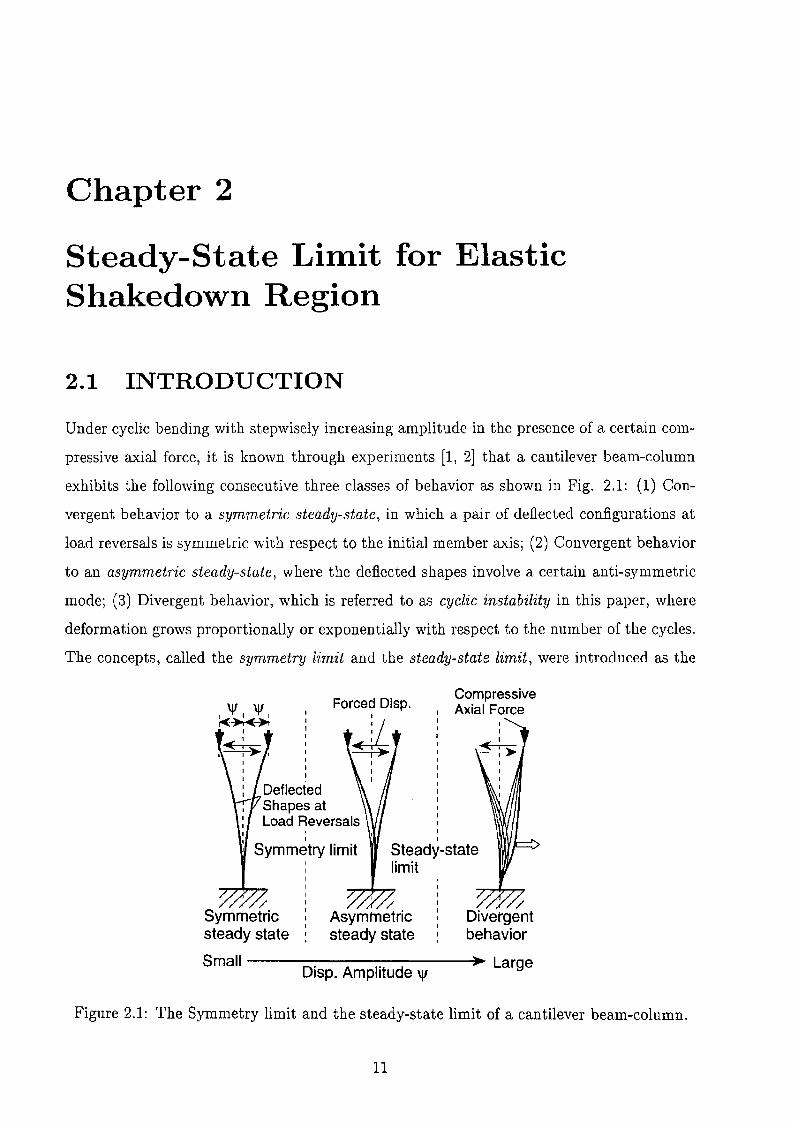
Under cyclic bending with stepwisely increasing amplitude in the presence of a certain com
pressive axial force, it is known through experiments [1, 2] that a cantilever beam-column
exhibits the following consecutive three classes of behavior as shown in Fig. 2.1: (1) Con
vergent behavior to a symmetric steady-state, in which a pair of deflected configurations at
load reversals is symmetric with respect to the initial member axis; (2) Convergent behavior
to an asymmetric steady-state, where the deflected shapes involve a certain anti-symmetric
mode; (3) Divergent behavior, which is referred to as cyclic instability in this paper, where
deformation grows proportionally or exponentially with respect to the number of the cycles.
The concepts, called the symmetry limit and the steady-state limit, were introduced as the
,,,,1
II
IIrI,,,,II
Steady-statelimit
DeflectedShapes atLoad Reversals
,Symmetry limit
IIII
I/: / /Symmetric I Asymtnetric Divergent
I
steady state : steady state behavior
Small -----------.....;)0... LargeDisp. Amplitude '"
Figure 2.1: The Symmetry limit and the steady-state limit of a cantilever beam-column.
11
critical steady states that bound these three classes of behavior. The symmetry limit is the
critical steady state at which transition from the symmetric steady state to the asymmetric
steady state occurs. The steady~state limit is the critical steady state beyond which the
beam-column will no longer exhibit any convergent behavior. To predict the symmetry limit
and the steady-state limit, the symmetry limit theory and the steady-state limit theory were
developed, respectively [1, 2, 3].
It might be thought that the symmetry limit and the steady-state limit can be found by
applying previously established theories. Nevertheless, none of them are directly applicable
for the following reasons: (1) Plastic buckling theory [4, 5]: The symmetry limit and the
steady-state limit are phenomenologically and conceptually different from the critical points,
such as a branching point and a limit point, of the equilibrium path. In other words, cyclic
instability may take place without passing the critical equilibrium points; (2) Shakedown
theory and its extensions: The symmetry limit and the steady-state limit are generally
observed under the strong effect of geometrical nonlinearity. In the classical shakedown theory
[6, 7], however, geometrical nonlinearity is completely neglected. Though several papers
[8, g, 10, 11, 12, 13, 14, 15, 16] extended the classical shakedown theory by taking geometrical
nonlinearity into account, the extended shakedown theories are not valid when compressive
stresses and/or large deformations have strong influence on the structural response, where
: Steady-StateVariables
Steady-State Path
~-- ----- _. -~--~ _. --~-
Equilibrium Path ina Transient Process
: Equilibrium StateVariables
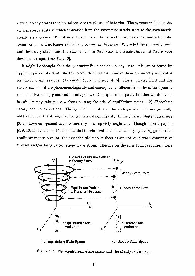
Closed Equilibrium Path ata Steady State \jf
(a) Equilibrium~State Space (b) Steady-State Space
Figure 2.2: The equilibrium-state space and the steady-state space.
12

structural responses are path-dependent; (3) Numerical methods for response analysis: It
is possible to bound convergence and divergence of plastic deformations (see e.g. [17, 18])
under specified loading histories. But a number of parametric analyses are required for
bounding the structural responses. Moreover, the parametric analyses will never lead to any
theoretical condition similar to that for the Euler load.
On the other hand, the symmetry limit and the steady-state limit can be found theo
retically, though under a specified loading history, in the symmetry limit theory and the
steady-state limit theory. The limits are found based on the following concepts. First, a
steady state is considered as a point in a special space schematically illustrated in Fig. 2.2.
Second, the sequence of these points, generated under an idealized cyclic loading program
with continuously increasing amplitude, is regarded as a continuous path. This path is called
the steady-state path. Third, the symmetry limit and the steady-state limit are found re
spectively as the first branching point and the first limit point of the steady-state path as
shown in Fig. 2.3. Since only the sequence of the steady states is traced, there is no need for
tracing the transient process between any pair of two adjacent steady states. Furthermore,
no parametric analysis is needed to detect the two limits because they are predicted as the
critical points of the steady-state path.
For a few classes of structures, the symmetry limit theory and the steady-state limit
theory have been applied. It was shown that severe cyclic instability is induced when the
deflection amplitude is in excess of the symmetry limit or the steady-state limit [2, 19]. In
those studies, however, only the simple structures, e.g. a cantilever beam-column or a unit
Steady-State Limit ~
--.... :Sequence of 1:J:jAsymmetricSteady States
/
VII!' viSequence of :Symmetric :Steady States /
Anti-Symmetric Component: vb (H I 2)
DivergentBehavior
I ~J
!
Figure 2.3: The symmetry limit and the steady-state limit in a steady-state plane.
13
frame, were treated for which analytical solutions can be derived. Hence, to investigate
the limit states of more complex and practical structures, which generally do not have a
symmetry limit if they do not have a symmetric shape, it is necessary to establish a method
for predicting the steady-state limit using appropriate finite element methods.
The purpose of this chapter is to present a new method for finding the steady-state limit
of elastoplastic trusses, which are one of the simplest finite dimensional structures, subjected
to initial constant loads and subsequent cyclic loads. In the following sections, governing
equations are described first. Then the fundamental concepts of the steady-state limit theory
are shown. Next, using the Taylor-series expansion, a new incremental theory is formulated
for tracing the steady-state path. Finally, validity of the proposed method is demonstrated
through numerical examples. The effects of the difference of loading histories on structural
responses are also shown in the numerical examples.
For simplicity, our consideration is restricted to the case in which dynamic and thermal
effects can be neglected. In addition, the scope of this chapter is limited to an elastic shake
down region because the problem becomes much more complicated when plastic shakedown
occurs in the trusses. Throughout this chapter, as referred in recent papers (see e.g. [9, 18]),
elastic shakedown or classic shakedown means a cyclic and fully elastic structural response
after some history of plastic deformations. And plastic shakedown is so called alternating
plasticity in which plastic deformations are included in steady cycles.
2.2 GOVERNING EQUATIONS
2.2.1 Analytical Model
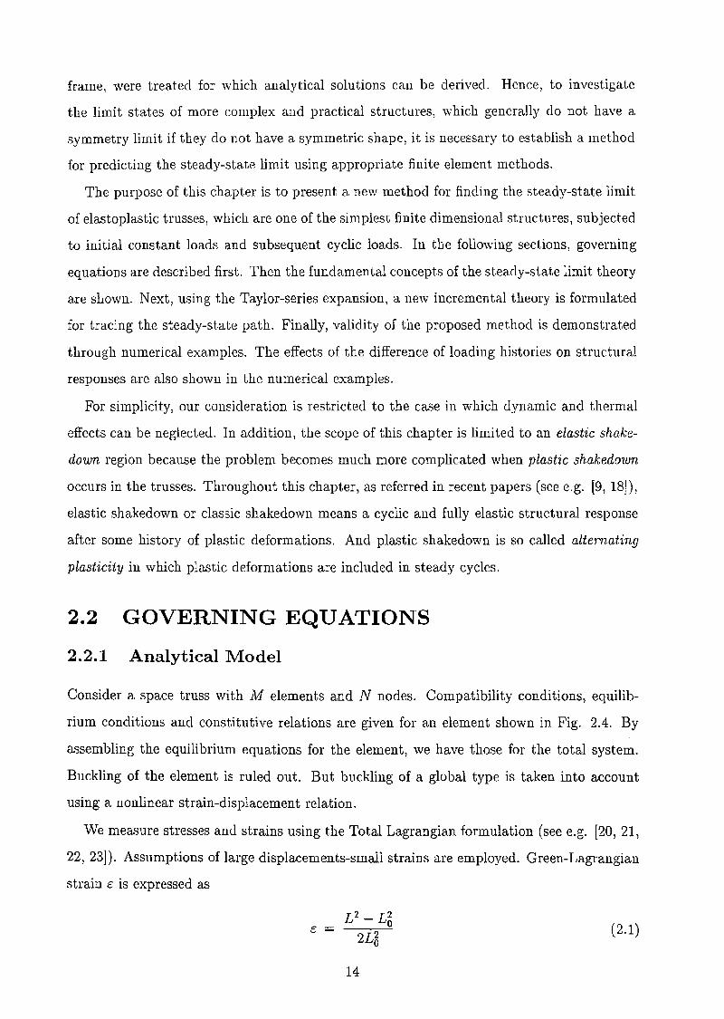
Consider a space truss with M elements and N nodes. Compatibility conditions, equilib
rium conditions and constitutive relations are given for an element shown in Fig. 2.4. By
assembling the equilibrium equations for the element, we have those for the total system.
Buckling of the element is ruled out. But buckling of a global type is taken into account
using a nonlinear strain-displacement relation.
We measure stresses and strains using the Total Lagrangian formulation (see e.g. [20, 21,
22, 23]). Assumptions of large displacements-small strains are employed. Green-Lagrangian
strain E is expressed as
E -2£6
14
(2.1)
I,I,
(x1' x2' x3 ) ... (U4. Us' u6 )I '
,/(u1' u2. u3) ...
x X~3 2,/ (XO,XO,XO)
~I EA,LO 4 S 6
(~, X~, xg) Initial Configuration
X1
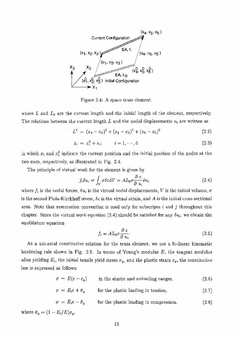
Figure 2.4: A space truss element.
where Land L o are the current length and the initial length of the element, respectively.
The relations between the current length L and the nodal displacements 1Li are written as
X~ +U'! ! 1 i = 1"",6
(2.2)
(2.3)
(2.4)
in which Xi and x? indicate the current position and the initial position of the nodes at the
two ends, respectively, as illustrated in Fig. 2.4.
The principle of virtual work for the element is given by
1 &cIioui = UOE:dV = ALou-&OUi
v Ui
where fi is the nodal forces, OUi is the virtual nodal displacements, V is the initial volume, U
is the second Piola-Kirchhoff stress, OE: is the virtual strain, and A is the initial cross sectional
area. Note that summation convention is used only for subscripts i and j throughout this
chapter. Since the virtual work equation (2.4) should be satisfied for any OUi, we obtain the
equilibrium equation
&cIi = ALou-& . (2.5)
Ui
As a um-axial constitutive relation for the truss element, we use a bi-linear bnematic
hardening rule shown in Fig. 2.5. In terms of Young's modulus E, the tangent modulus
after yielding EtJ the initial tensile yield stress uY1 and the plastic strain cp, the constitutive
law is expressed as follows:
in the elastic and unloading ranges, (2.6)
u
u
for the plastic loading in tension,
for the plastic loading in compression.
(2.7)
(2.8)
where ay = (1 - EdE)uy.
15

2.2.2 Cyclic Responses
For later formulation of the steady-state limit theory, we must examine all possible types
of the cyclic responses in the stress-strain plane. Possible cyclic responses are classified into
four different types E, C, T and P as shown in Fig. 2.6, where the superscripts t and c
indicate the state variables, such as stresses, strains, and displacements, at strain reversals
in tension and compression, respectively. In terms of (Et, at) and (Ec , aC), the cyclic responses
can be uniquely described as:
(2.9)
(2.10)
for type E, which represents a purely elastic response or an elastic shakedown state.
(2.11)
(2.12)
for type T, which is the elastic shakedown state whose maximum stress reaches the tensile
yield stress.
E C -tC - ay
(2.13)
(2.14)
for type C, which represents the elastic shakedown state that starts from and reaches the
compressive strain hardening line. Though all the possible types are shown in Fig. 2.6, type
oI,
rIIrII
cr = Et E + (1 :- Et / E) cry---_.-----
--=== Et1
E
-----------
Figure 2.5: A bi-linear kinematic hardening rule.
16

TypeC
Type T Type P
Figure 2.6: Possible types of cyclic responses.
P is not considered in this chapter because the discussion is limited to the elastic shakedown
region as mentioned in the introduction.
Note that the plastic strain cp is eliminated in Eqs. (2.12) and (2.13). For type T, (Jt is
expressed in two ways using Eqs. (2.6) and (2.7), while (JC is written using only Eq. (2.6).
The plastic strains at the strain reversals is eliminated using these three expressions and the
following relation
(2.15)
For type C, the plastic strain can be eliminated similarly.
2.3 FUNDAMENTAL CONCEPTS
2.3.1 Loading Conditions
The truss is subjected to initial constant loads AOPo and subsequent cyclic loads AcPc. Here,
A and P denote the load factor and the constant vector, respectively. The subscripts 0 and
c indicate that the variables refer to the constant loads and to the cyclic loads, respectively.
External forces and/or forced displacements are applied as the external loads. In other
words, nodal forces and/or nodal displacements are included in P. The load factor Ac is
varied between the maximum value A~ = 'l/J and the minimum value A~ = -'l/J in a cycle)
where'l/J denotes the amplitude of Ac. The equilibrium states at which Ac = A~ and Ac = A~
are called r 1 state and r n state, respectively. The superscripts I and II indicate that the
state variables refer to those for the r1 and rn states, respectively.
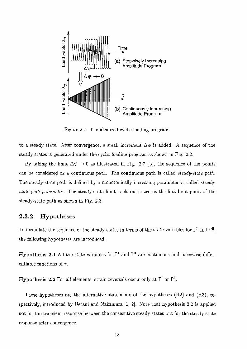
As a preliminary program, consider a cyclic loading program shown in Fig. 2.7 (a). In the
program, the loading cycle is repeated as many times as necessary for the truss to converge
17
..-::0....ot5ctl
LL"'Cctl
S
Time
(a) Stepwisely IncreasingAmplitude Program
t
(b) Continuously IncreasingAmplitude Program
Figure 2.7: The idealized cyclic loading program.
to a steady state. After convergence, a small increment ~'ljJ is added. A sequence of the
steady states is generated under the cyclic loading program as shown in Fig. 2.2.
By taking the limit t1'ljJ ---+ 0 as illustrated in Fig. 2.7 (b), the sequence of the points
can be considered as a continuous path. The continuous path is called steady-state path.
The steady-state path is defined by a monotonically increasing parameter T, called steady
state path parameter. The steady-state limit is characterized as the first limit point of the
steady-state path as shown in Fig. 2.3.
2.3.2 Hypotheses
To formulate the sequence of the steady states in terms of the state variables for r T and r D,
the following hypotheses are introduced:
Hypothesis 2.1 All the state variables for r I and r n are continuous and piecewise differ
entiable functions of T.
Hypothesis 2.2 For all elements, strain reversals occur only at r I or rD.
These hypotheses are the alternative statements of the hypotheses (H2) and (H3), re
spectively, introduced by Uetani and Nakamura [1, 2]. Note that hypothesis 2.2 is applied
not for the transient response between the consecutive steady states but for the steady state
response after convergence.
18
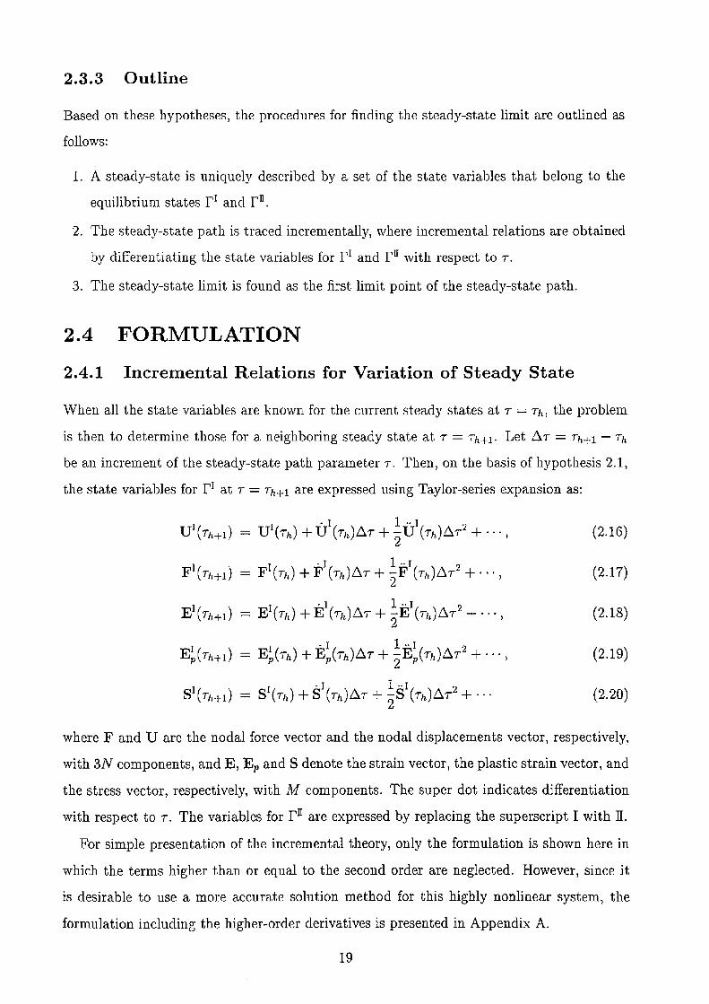
2.3.3 Outline
Based on these hypotheses, the procedures for finding the steady-state limit are outlined as
follows:
1. A steady-state is uniquely described by a set of the state variables that belong to the
equilibrium states r I and r II •
2. The steady-state path is traced incrementally, where incremental relations are obtained
by differentiating the state variables for r l and r II with respect to T.
3. The steady-state limit is found as the first limit point of the steady-state path.
2.4 FORMULATION
2.4.1 Incremental Relations for Variation of Steady State
When all the state variables are known for the current steady states at T = Tit, the problem
is then to determine those for a neighboring steady state at T = Th+l' Let 6.T = ThH - Th
be an increment of the steady-state path parameter T. Then, on the basis of hypothesis 2.1,
the state variables for r l at T = Th+! are expressed using Taylor-series expansion as:
I 1'1 1,,1 ?
U (Th+d = U (Th) + U (Th)6.T +"2U (Th)6.T~+"',
I 1'1 1"1 2F (Th+!) = F (Th) +F (Th)6.T + "2F (Th)6.T +"',
I I·J 1"1 2E (Th+d = E (Th) + E (Th)6.T + "2E (Th)6.T +"',
I 1'1 1,,1 2Ep(Th+d = Ep(Th) + Ep(Th)6.T + "2 Ep (Th)6.T +"',
I 1.1 1"1 28 (Th+d = 8 (Til) + 8 (Th)LlT + "28 (Th)6.T + ...
(2.16)
(2.17)
(2.18)
(2.19)
(2.20)
where F and U are the nodal force vector and the nodal displacements vector, respectively,
with 3N components, and E, E p and 8 denote the strain vector, the plastic strain vector, and
the stress vector, respectively, with M components. The super dot indicates differentiation
with respect to T. The variables for r IT are expressed by replacing the superscript I with II.
For simple presentation of the incremental theory, only the formulation is shown here in
which the terms higher than or equal to the second order are neglected. However, since it
is desirable to use a more accurate solution method for this highly nonlinear system, the
formulation including the higher-order derivatives is presented in Appendix A.
19

2.4.2 Rate Forms of Governing Equations
By differentiating all the governing equations for r l and r lI with respect to the steady
state parameter T 1 we derive the rate form of the governing equations. The rate forms of the
governing equations are simply called rate equations in this chapter. Differentiation of the
compatibility conditions (2.1)-(2.3) yields
.1 a [1 . I
[ = 8 Ui1ui , (2.21)
(2.22)
Recall that summation convention is used only for the subscripts i, j and k which are varied
from 1 to 6. Rate forms of the equilibrium conditions are given by
(a 1 82
I )'1 . I [ 1 [ ·1f i = ALa (]" a UiI + (]" aUiI a UjI u j ,
(8 rr a? rr )'rr . rr [ 1I ~ [ • IT
fi = ALa (]" -8rr + (J a rr a rr uj .Ui Ui Uj
(2.23)
(2.24)
Differentiating the stress-strain relations (2.9)-(2.12)1 the stress rate-strain rate relations can
be expressed for the strain-reversal points in the form of
(2,25)
(2.26)
cr
---- ----------
0:
----------
T .... T (Et~ 0) T.... E (tt <0)
cr
E.... E
o : (Et(th)' crt(th))
• : (EC(th), crc('th))
o : (Et(th+1)' crt(th+1))
• : (EC(th+1)' crc(th+1))
Figure 2.8: Possible types of the variation of cyclic responses.
20
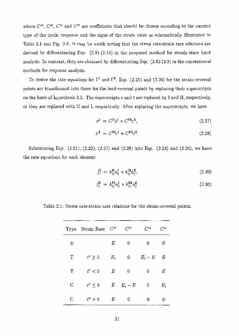
where ecc , eet, etc and C tt are coefficients that should be chosen according to the current
type of the cyclic response and the signs of the strain rates as schematically illustrated in
Table 2.1 and Fig. 2.8. It may be worth noting that the stress rate-strain rare relations are
derived by differentiating Eqs. (2.9)-(2.14) in the proposed method for steady-state limit
analysis. In contrast, they are obtained by differentiating Eqs. (2.6)-(2.8) in the conventional
methods for response analysis.
To derive the rate equations for r I and r IT , Eqs. (2.25) and (2.26) for the strain-reversal
points are transformed into those for the load-reversal points by replacing their superscripts
on the basis of hypothesis 2.2. The superscripts c and t are replaced by I and II, respectively,
or they are replaced with II and I, respectively. After replacing the superscripts, we have
(2.27)
(2.28)
Substituting Eqs. (2.21), (2.22), (2.27) and (2.28) into Eqs. (2.23) and (2.24), we have
the rate equations for each element
(2.29)
(2.30)
Table 2.1: Stress rate-strain rate relations for the strain-reversal points.
Type Strain Rate Ctt etc ect GCc
E E 0 0 E
T it ~ 0 Et 0 Et -E E
T it < 0 E 0 0 E
C i C .s; 0 E Et-E a Et
c i C > 0 E 0 0 E
21

where
k~~1)
(2.31)
(2.32)
(2.33)
k~.n = ALa (cnn 8 en CJ ell + (lII 82
ell ) (2.34)1) 8 UjD 8 u}' [) Ui ll [) UjD .
By assembling Eqs. (2.29) and (2.30) throughout the whole structure, the following rate
equations are derived for the total system:
(2.35)
(2.36)
where K II, KIll, K llI and K llll are the coefficient matrices of the nodal displacement rates. By
specifying 1/J and by using the boundary conditions, we have a system of 2 x 3N simultaneous
linear equations.
2.4.3 Consistent Set of Stress Rate-Strain Rate Relations
When an element exhibits type T or type C behavior, the coefficients of the strain rates
should be chosen according to the signs of the strain rates as shown in Table 2.1 and Fig.
2.8. Therefore, for all the elements exhibiting the type T or the type C behavior, we should
choose a set of the coefficients that are consistent with the signs of the resulting strain rates.
Note that the term consistent used here has no relation with the one used in integration
algorithms for the numerical response analysis of elastoplastic solids or structures (see e.g.
[24, 25]).
To find the consistent set of the coefficients, we employ a trial and error approach, which
is also used in the conventional response analysis [26]. In the trial and error approach, first 1
the signs of the strain rates E1and Ell are assumed to be equal to those in the last step.
Then, the coefficients cee, Cet , Cte and Ctt are determined according to the assumptions,
. I . nand the rate equations are constructed. After the rate equations are solved and E and E
are calculated, the consistency is checked between the assumed signs of the strain rates and
the resulting ones for all the elements exhibiting the type T or the type C behavior. If the
signs are not consistent, the assumed signs are reversed. This procedure is continued until
all the resulting signs of the strain rates are consistent with the assumed ones.
22
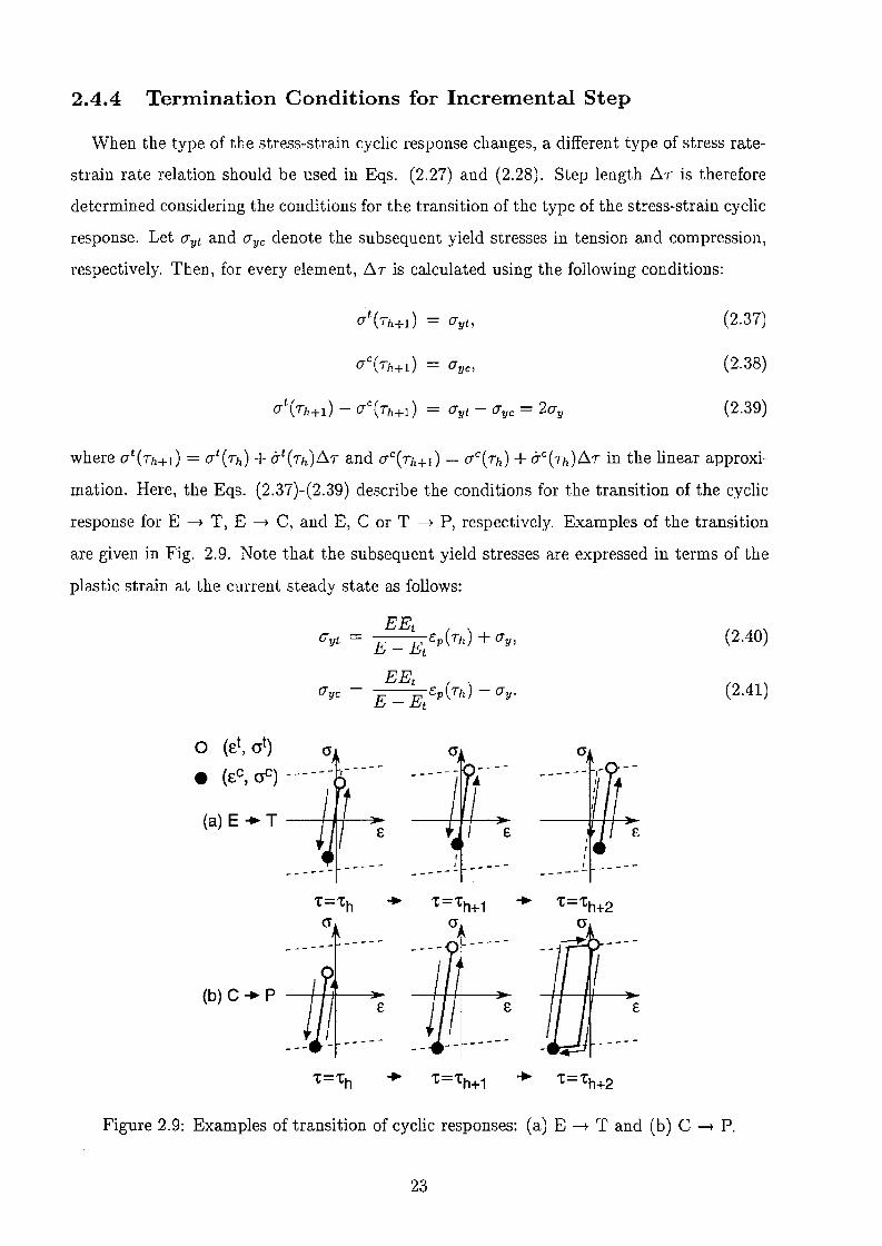
2.4.4 Termination Conditions for Incremental Step
When the type of the stress-strain cyclic response changes, a different type of stress rate
strain rate relation should be used in Eqs. (2.27) and (2.28). Step length 6.T is therefore
determined considering the conditions for the transition of the type of the stress-strain cyclic
response. Let O"yt and O"yc denote the subsequent yield stresses in tension and compression,
respectively. Then, for every element, 6.T is calculated using the following conditions:
(7t (Th+1) = (7yt, (2.37)
(2.38)
(2.39)
where (7t(Th+l) = CTt(Th) + o-t(Th).6.T and O"C(Th+d = CTC(Th) + o-C(Th)6.T in the linear approxi
mation. Here, the Eqs. (2.37)-(2.39) describe the conditions for the transition of the cyclic
response for E -----Jo T, E -----Jo C, and E, C or T -----Jo P, respectively. Examples of the transition
are given in Fig. 2.9. Note that the subsequent yield stresses are expressed in terms of the
plastic strain at the current steady state as follows:
EEtO"yt = E _ E
tEp(Th) + CTYl
EEtCT yc E _ E
tEp(Th) - CTy .
(2.40)
(2.41)
crcr
---- ----------
't='th .. 't='th+1 .. 't='th+2cr cr cr
----- -_ ... --
(b) C .. PE E £
_... -- ----
't='th .. 't='th+1 .. 't='th+2
(a) E .. T --HH-~E
a (ct, crt) cr• (cC, crC) - ~ - -- - ,- - ---
Figure 2.9: Examples of transition of cyclic responses: (a) E -----Jo T and (b) C -----Jo P.
23

Besides the conditions above, the step length 6.7 should be kept small enough to prevent
excessive accumulation of truncation errors. Hence the step length 6.7 is selected as the
smallest value among the values calculated from the conditions (2.37)-(2.39) and the specified
maximum allowable value 6.fmax . \iVhen 6.7 is determined by (2.37) or (2.38), the stress
rate-strain rate relations are changed in the next step. When (2.39) is used to determine
b..T, the incremental analysis is terminated.
2.4.5 Steady-State Limit Condition
Now, all the first-order derivatives and the step length b..T have been obtained. Substituting
6.7 and the first-order derivatives into Eqs. (2.16)-(2.20), we have all the state variables at
7 = Th+l' Repeating these procedures, the steady-state path is traced incrementally.
As mentioned before, the steady-state limit is defined as the first limit point of the steady
state path as shown in Fig. 2.3. The steady-state limit condition is given as
(2.42)
Note that, to find the limit point and to trace the steady-state path after the limit point, an
procedure should be employed similar to displacement control schemes [26, 22].
2.5 NUMERICAL EXAMPLES
The proposed method has been developed on the basis of the two hypotheses. Moreover the
steady-state limit is predicted regardless of the transient process between the two consecutive
steady states. Hence validity of the two hypotheses and the steady-state limit should be
examined. For this purpose, both steady-state limit analysis and conventional response
analysis, in which the entire history is traced, are carried out for a two-bar arch truss and a
ten-bar cantilever truss. And the results of the analyses are compared. In addition, the effect
of the differences of the loading histories are discussed through these numerical examples.
2.5.1 Steady-State Limit Analysis
Initial shape, boundary conditions and loading conditions of both plane trusses are illustrated
in Fig. 2.10. The initial constant forces and the subsequent cyclic forced displacements are
denoted by AOPOand AXle, respectively. Here, Po = 9.807 x 10³N and Ue = 1cm. The
cross-sectional areas of the two-bar truss are A(l) = 1 cm2 and A(2) = 2 cm2, and those
of the ten-bar truss are as follows: A(l) = A(4) = A(5) = 11 cm2, A(2) = A(3) = 1.1 cm2
,
24
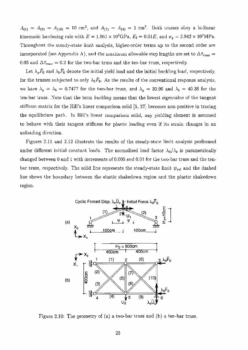
A(6) = A(9) = A(1o) = 10 cm2, and A(7) = A(8) = 1 cm2. Both trusses obey a bi-linear
kinematic hardening rule with E = 1.961 x 10²GPa, Et = O.OIE, and CJy = 2.942 x 10²MPa.
Throughout the steady-state limit analysis, higher-order terms up to the second order are
incorporated (see Appendix A), and the maximum allowable step lengths are set to .6.Tmux =
0.05 and l':.fmux = 0.2 for the two-bar truss and the ten-bar truss, respectively.
Let AyFo and AbFO denote the initial yield load and the initial buckling load, respectively,
for the trusses subjected to only AoFo. As the results of the conventional response analysis,
we have Ay = Ab = 0.7477 for the two-bar truss, and Ay = 30.96 and Ab = 40.38 for the
ten-bar truss. Note that the term buckling means that the lowest eigenvalue of the tangent
stiffness matrix for the Hill's linear comparison solid [5, 27] becomes non-positive in tracing
the equilibrium path. In Hill's linear comparison solid, any yielding element is assumed
to behave with their tangent stiffness for plastic loading even if its strain changes in an
unloading direction.
Figures 2.11 and 2.12 illustrate the results of the steady-state limit analysis performed
under different initial constant loads. The normalized load factor Ao/ Ab is parametrically
changed between 0 and 1 with increments of 0.005 and 0.01 for the two-bar truss and the ten
bar truss, respectively. The solid line represents the steady-state limit 'l/Jssl and the dashed
line shows the boundary between the elastic shakedown region and the plastic shakedown
region.
(a) 1 '1'1 !JX2
100cm 100cm
LX1
~
H2 =aOOcm400cm T 4QQcmr- X2
Xl
EU
(b)00'l:t
1.01=06
AcUc
Figure 2.10: The geometry of (a) a two-bar truss and (b) a ten-bar truss.
25

1.0.0~
~ 0.8~
~ 0.6oU-rn 0.4Ec
0.2
00
(9.276 x 10-; 0.5) -I
/!Boundary between iElastic and Plastic !Shakedown \
3 6 9 12
Amplitude: \jI / H 1
Figure 2.11: The elastic shakedown boundaries for the two-bar truss.
1.2 ...-----.---...-----.---...---....,
1.0
--o 0.8~
~ 0.6oU-rn 0.4c
0.2
Steady-State Limit CurveAo/Ab =0.88
Convergenceunder STIDAD~
fI
l;)
Boundary between 1
Elastic and Plastic IShakedown i
~i\
1 2 3 4
Amplitude: 'JI / H2
Figure 2.12: The elastic shakedown boundaries for the ten-bar truss.
26
2.5.2 Response Analysis
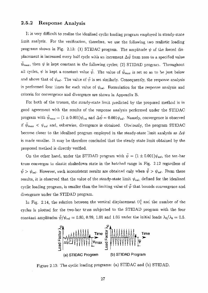
It is very difficult to realize the idealized cyclic loading program employed in steady-state
limit analysis. For the verification, therefore, we use the following two realistic loading
programs shown in Fig. 2.13: (1) STIDAC program. The amplitude 1/J of the forced dis~
placement is increased every half cycle with an increment .6.'0 from zero to a specified value
if;max, then 1/J is kept constant in the following cycles; (2) STIDAD program. Throughout
all cycles, 'IjJ is kept a constant value '0. The value of ifmax is set so as to be just below
and above that of 'l/Jss/. The value of '0 is set similarly. Consequently, the response analysis
is performed four times for each value of 7/Jss/' Formulation for the response analysis and
criteria for convergence and divergence are shown in Appendix B.
For both of the trusses, the steady-state limit predicted by the proposed method is in
good agreement with the results of the response analysis performed under the STIDAC
program with 7jJmax = (1 ± O.OOl)7/Jssl and .6.7jJ = O.OOl7/Jss/' Namely, convergence is observed
if '0max < 'l/Jss/ and, otherwise, divergence is obtained. Obviously, the program STIDAC
become closer to the idealized program employed in the steady-state limit analysis as .6.7/J
is made smaller. It may be therefore concluded that the steady state limit obtained by the
proposed method is directly verified.
On the other hand, under the STIDAD program with if = (1 ± O.OOl)Wss/, the ten-bar
truss converges to elastic shakedown state in the hatched range in Fig. 2.12 regardless of
if; > 'l/Jssl' However, such inconsistent results are obtained only when 1jj > Wssl' From these
results, it is observed that the value of the steady-state limit 7/Jssl, defined for the idealized
cyclic loading program, is smaller than the limiting value of ijJ that bounds convergence and
divergence under the STIDAD program.
In Fig. 2.14, the relation between the vertical displacement uI and the number of the
cycles is plotted for the two-bar truss subjected to the STIDAD program with the four
constant amplitudes 7jJ/'l/Jssl = 0.80, 0.99, 1.01 and 1.05 under the initial loads >'0/Ab = 0.5.
Time
(a) STIDAC Program (b) STIDAD Program
Figure 2.13: The cyclic loading programs: (a) STIDAC and (b) STIDAD.
27

It can be observed from Fig. 2.14 that cyclic instability occurs if the amplitude '1/) is above
the predicted value of tPss[, whereas vI converges otherwise.
Figure 2.15 illustrates comparison of the results for the ten-bar truss obtained by the
steady-state limit analysis and the response analyses performed under various cyclic load
ing programs under the initial constant load 'Ao/ Ab = 0.85. This figure shows the path-
1.01'Vssl
.....::> -0.1
0.~oCO -0.2otCD>
I-o Gt-----...,---------.-------,
5 10Number of cycles
15
Figure 2.14: Convergence and divergence of VI for the two-bar truss (A/ Ab = 0.5).
Steady-State Path
C\I
I :-'\_.._._._-- 2~ 'VsslQ)
""0::s
~.'!:::a.E 1 STIDAD«
(X10-3)
3 r-~---o~-r-----r-----r-------,
\ 0 0 STIDAC withLimiting Value Large 'Vmaxfor STIDAD ':-.-~_-------~--------------
"JOoII
-~-- ~--_ ...~-,"--
//'/
,~"
,.."o './
///'
,/
""i'
21oO'-- ~--_....I.--_-......L..--_.....I
-1
Figure 2.15: Path dependence of Vi on loading history for the ten-bar trusses ('A/ Ab = 0.85).
28

dependence on loading history of the limiting value that bounds convergence and divergence.
In the figure, U2 is the displacement of node 5 for Xl direction. The solid line indicates the
steady-state path. The dashed line shows the variation of U~ \vith respect to 1/) under STI
DAC program with 6.ij; = O.OOl7./Jssl and a sufficiently large value of 7Pmax. The circular
symbols plot UJ in the steady states under the STIDAC programs with 6.i/J = O.OO11/)ssl and
various values of i/Jmax. The square symbols indicate U~ after convergence under the STIDAD
programs with the values of 7P corresponding to the values of i/Jmax. Good agreement between
the steady-state path and the circular points demonstrates the validity of the hypotheses
(H2·) and (H3*).
2.6 CONCLUSIONS
A new method has been presented for predicting the steady-state limit of elastoplastic trusses
subjected to quasi-static cyclic loads in the presence of constant loads. By applying the
proposed method, we can find the steady-state limit of arbitrary shaped frames with truss
and/or fiber elements. In the proposed method, there is no need for tracing the transient
process between consecutive steady states, and no parametric analysis is needed for finding
the steady-state limit. The proposed method is therefore much more efficient than the
conventional methods for numerical response analysis.
Through the numerical examples, the following conclusions have been obtained:
1. Good agreement is observed between the results of the steady-state limit analysis and
those of the conventional response analysis when the loading conditions for these anal
yses are close.
2. The limiting values below which elastic shakedown occurs depend on the loading history.
Obviously, Melan-type or path-independent shakedown criterion cannot be extended to
such cases.
3. The steady-state limits, defined under an idealized cyclic loading program with continu
ously increasing amplitude, provide lower bounds for the limiting values obtained by the
response analysis performed under the two typical and realistic cyclic loading programs.
29
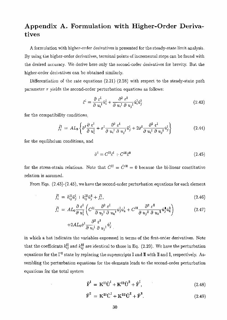
Appendix A. Formulation with Higher-Order Derivatives
A formulation with higher-order derivatives is presented for the steady-state limit analysis.
By using the higher-order derivatives, terminal points of incremental steps can be found with
the desired accuracy. We derive here only the second-order derivatives for brevity. But the
higher-order derivatives can be obtained similarly.
Differentiation of the rate equations (2.21)-(2.28) with respect to the steady-state path
parameter T yields the second-order perturbation equations as follows:
for the compatibility conditions,
{a I 82 I 82 I }'1 ··1 £ 1 £ ..1 . I £ . 1
Ii = ALo a -8~ + a a .1 8 .I u j + 20" a .I 8 .I ujU1. U1. uJ U1. UJ
for the equilibrium conditions, and
•• J ell ..I eIII "na= e+ £
(2.43)
(2.44)
(2.45)
for the stress-strain relations. Note that err = e III = 0 because the bi-linear constitutive
relation is assumed.
From Eqs. (2.43)-(2.45), we have the second-order perturbation equations for each element
(2.46)
(2.47)
in which a hat indicates the variables expressed in terms of the first-order derivatives. Note
that the coefficients kg and klJ are identical to those in Eq. (2.29). We have the perturbation
equations for the r nstate by replacing the superscripts I and IT with IT and I, respectively. As
sembling the perturbation equations for the elements leads to the second-order perturbation
equations for the total system
.. r rr"I moon ~IF = K U +K U +F,
.. n nr " I nn .. n ~ nF=KU+KU+F.
30
(2.48)
(2.49)
Note again that the coefficient matrices are same as those in the rate equations (2.35) and
(2.36). These 2 x 3N simultaneous linear equations (2.48) and (2.49) are to be solved using
the boundary conditions after the value of '1/) is specified.
When the derivatives are employed up to the second order, the termination conditions
Eqs. (2.37)-(2.39) of the incremental step become quadratic equations of the step length 6.7,
while the conditions are linear equations when only the first derivatives are used. Besides
these termination conditions, we must consider the conditions
(2.50)
(2.51)
for the transitions T ---t E and C ---t E, respectively. Note that, by using the higher-order
terms, we do not have to find the consistent set of stress rate-strain rate relations as far as no
discontinuous change occurs in the derivatives with respect to T. But, if the discontinuous
change occurs, e.g. types of the cyclic stress-strain response changes, the consistent set
should be found at the moment.
Substituting the step length and the derivatives up to the second order into Eqs. (2.16)
(2.20), we obtain the values of the state variables at 7 = Th+l'
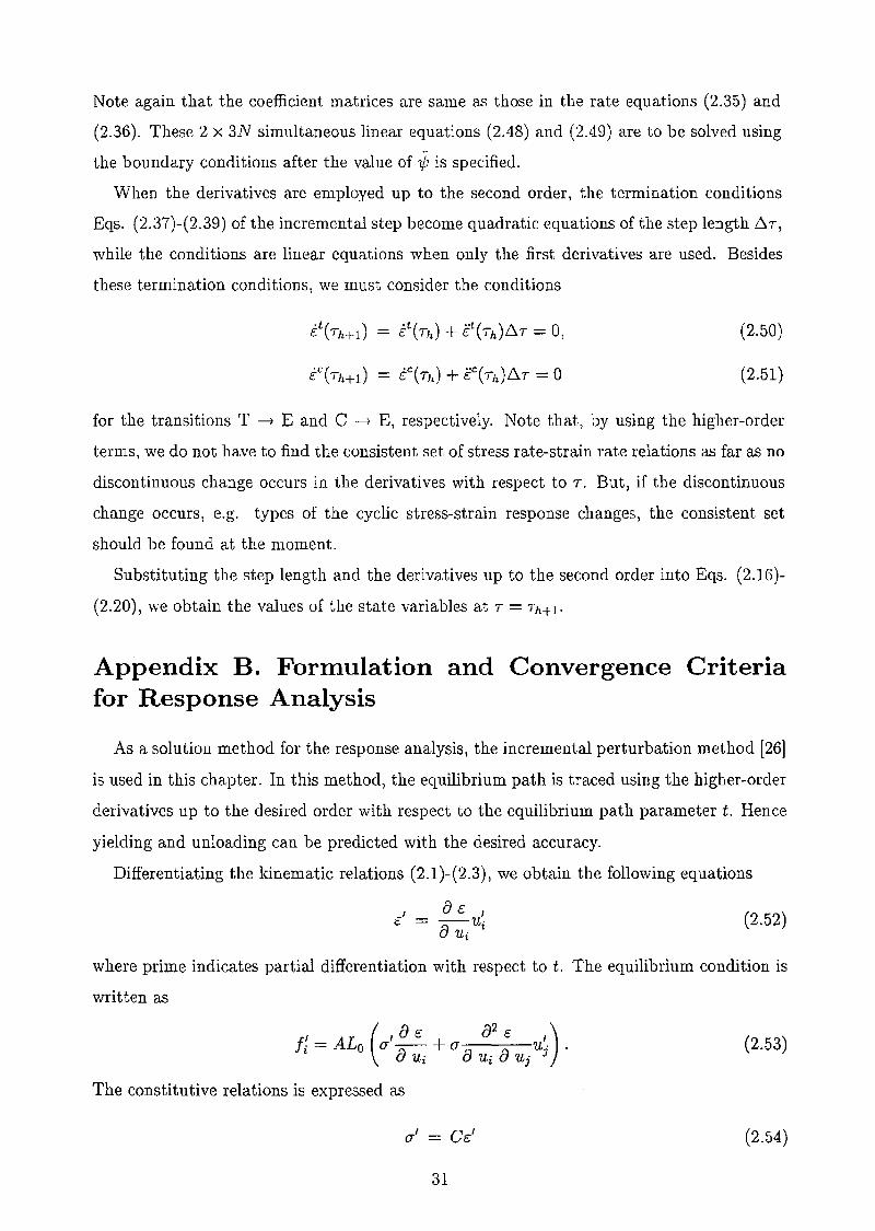
Appendix B. Formulation and Convergence Criteriafor Response Analysis
As a solution method for the response analysis, the incremental perturbation method [26]
is used in this chapter. In this method, the equilibrium path is traced using the higher-order
derivatives up to the desired order with respect to the equilibrium path parameter t. Hence
yielding and unloading can be predicted with the desired accuracy.
Differentiating the kinematic relations (2.1)-(2.3), we obtain the following equations
I 8 £. I£. = --u,
8 Ui t(2.52)
where prime indicates partial differentiation with respect to t. The equilibrium condition is
written as
I AL ( I 8 £. 82
£. ,)Ii = 0 a- 8 Ui + (J 8 Ui 8 Uj Uj .
The constitutive relations is expressed as
a-I = G£.'
31
(2.53)
(2.54)
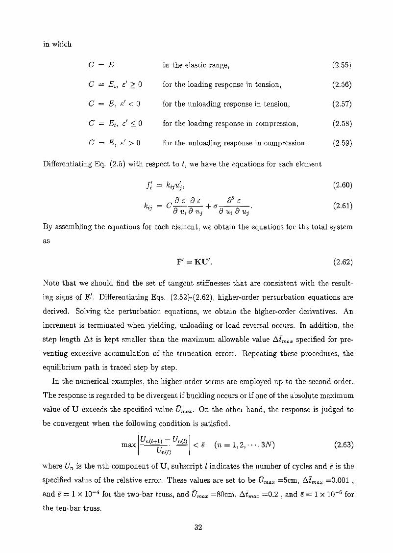
in which
C=E in the elastic range~ (2.55)
C EL, E' ~ 0 for the loading response in tension, (2.56)
C E, E' < 0 for the unloading response in tension, (2.57)
C ELl S' ~ 0 for the loading response in compression, (2.58)
C - E, E' > 0 for the unloading response in compression. (2.59)
Differentiating Eq. (2.5) with respect to t, we have the equations for each element
II (2.60)
(2.61)kij
= C 8 E~ + a 82
E
8 Ui 8 Uj 8 Ui 8 Uj
By assembling the equations for each element, we obtain the equations for the total system
as
(2.62)
(2.63)
Note that we should find the set of tangent stiffnesses that are consistent with the result
ing signs of E'. Differentiating Eqs. (2.52)-(2.62), higher-order perturbation equations are
derived. Solving the perturbation equations, we obtain the higher-order derivatives. An
increment is terminated when yielding, unloading or load reversal occurs. In addition, the
step length 6.t is kept smaller than the maximum allowable value b.tmax specified for pre
venting excessive accumulation of the truncation errors. Repeating these procedures, the
equilibrium path is traced step by step.
In the numerical examples, the higher-order terms are employed up to the second order.
The response is regarded to be divergent if buckling occurs or if one of the absolute maximum
value of U exceeds the specified value Umax . On the other hand, the response is judged to
be convergent when the following condition is satisfied.
max Un(l+l) - Un(l) < e (n = 1,2, ... ,3N)Un(l)
where Un is the nth component of U, subscript I indicates the number of cycles and e is the
specified value of the relative error. These values are set to be Umax =5cm, b.tmax =0.001 ,
and e= 1 x 10⁻⁴ for the two-bar truss, and Umax =80cm, b.tmax =0.2 1 and e = 1 x 10⁻⁶ for
the ten-bar truss.
32
Nomenclature
The following symbols are used in this chapter:
A initial cross sectional area;
e coefficient of E';
ett ete eet eee coefficients of it and i C:
, , , I
ell em eill euu coefficients of i 1and in,'I I ,
E Young's modulus;
E t tangent modulus after yielding;
E strain vector for total system;
Ep plastic strain vector for total system;
e specified value of relative error;
F nodal force vector for total system;
Ii nodal force;
H Height of truss;
K tangent stiffness matrix;
K II KIll K IIl KnIT coefficient matrices of (l and ll·,, ,
kij coefficient of uj;
k~~ k~~ k~~ k~)l coefficients of uJI and uJ~:ZJ ZJ' ZJ I ZJ '
L current length;
L o initial length;
M number of elements;
N number of nodes;
Po constant vector for constant loads;
Pc constant vector for cyclic load;
S stress vector for total system;
t equilibrium path parameter;
U nodal displacement vector for total system;
Umax maximum allowable value of Un;
Un(l) nth component of U at lth cycle;
Ui nodal displacement;
33

V initial volume;
Xi current position of nodes;
x? initial position of nodes;
c Green-Lagrangian strain;
cp plastic strain;
AO load factor for constant load;
Ab load factor at initial buckling load;
Ac load factor for cyclic loads;
Ay load factor at initial yielding load;
(J" second Piola-Kirchhoff stress;
(J"y initial tensile yield stress;
o-y O"y = (1 - EdE)(J"y;
(J"yc subsequent yield stress in compression;
(J"yt subsequent yield stress in tension;
T steady-state path parameter;
Th T at h step;
t3.t increment of equilibrium path parameter;
t3.tmax maximum allowable value of t3.t;
t3.T increment of steady-state path parameter;
t3.Tmax maximum allowable value of t3.T;
t3.7/J increment of amplitude;
t3.'0 specified increment of amplitude for STIDAC program;
Dc virtual strain;
6Ui virtual nodal displacement;
7/J amplitude of Ac ;
'lj)ssl amplitude at steady-state limit;
iii constant amplitude for STIDAD program; and
'0max maximum amplitude for STIDAC program.
Superscripts
t variables for t,he equilibrium states at strain reversals in tension;
34

c variables for the equilibrium states at strain reversals in compression;
I variables for the equilibrium states at Ac = 'lj;i and
1I variables for the equilibrium states at Ac = -'Ij;.
Signs
() derivatives with respect to Ti
() second order derivatives with respect to T;
(~) quantities expressed with first-order derivatives with respect to Ti and.
()' derivatives with respect to t.
35
References
[1] K. Uetani and T. Nakamura. Symmetry limit theory for cantilever beam-columns sub
jected to cyclic reversed bending. Journal of the Mechanics and Physics of Solids,
31(6):449-484, 1983.
[2] K. Uetani. Symmetry Limit Theory and Steady-State Limit Theory for Elastic-Plastic
Beam-Columns Subjected to Repeated Alternating Bending. PhD thesis, Kyoto Univer
sity, 1984. (in Japanese).
[3] K. Uetani. Uniqueness criterion for incremental variation of steady state and symmetry
limit. Journal of the Mechanics and Physics of Solids, 37(4):495-514, 1989.
[4] F. R. Shanley. Inelastic column theory. Journal of Aeronautical Sciences, 14:261-268,
1947.
[5] R. Hill. A general theory of uniqueness and stability in elastic-plastic solids. Journal of
the Mechanics and Physics of Solids, 6:236-249, 1958.
[6] W. T. Koiter. General theorems for elastic-plastic structures. In J. N. Sneddon and
R. Hill, editors, Progress in Solid Mechanics, volume 1, pages 167-221, North Holland,
Amsterdam, 1960.
[7] J. A. Konig. Shakedown of Elastic-Plastic Structures. Elsevier, Amsterdam, 1987.
[8] G. Maier. A shakedown matrix theory allowing for workhardening and second-order
geometric effects. In A. Sawczuk, editor, Foundations of plasticity, volume 1, pages
417-433, Noordhoff, Leyden, 1972.
[9] Q. S. Nguyen, G. Gary, and G. Baylac. Interaction buckling-progressive deformation.
Nuclear Engineering and Design, 75:235-243, 1983.
[10] A. Siemaszko and J. A. Konig. Analysis of stability of incremental collapse of skeletal
structures. Journal of Structural Mechanics, 13:301-321, 1985.
[11] D. Weichert. On the influence of geometrical nonlinearities on the shakedown of elastic
plastic structures. International Journal of Plasticity, 2:135-148, 1986.
[12] J. Gross-Weege. A unified formulation of statical shakedown criteria for geometrically
nonlinear problems. International Journal of Plasticity, 6:433-447, 1990.
[13] S. Pycko and J. A. Konig. Steady plastic cycles on reference configuration in the
presence of second-order geometric effects. European Journal of Mechanics. A, Solids,
10(6), 1991.
[14] H. Stumpf. Theoretical and computational aspects in the shakedown analysis of finite
elastoplasticity. International Journal of Plasticity, pages 583-602, 1993.
36
[15] Z. Mroz, D. Weichert, and S. Dorosz, editors. Inelastic Behavior of Structures ~mder
Variable Loads. Kluwer Academic Publishers, Netherlands, 1995.
[16] C. Polizzotto and G. Borio. Shakedown and steady-state responses of elastic-plastic
solids in large displacements. International Journal of Solids and StructuTes, 33:3415
3437, 1996.
[17] K. Morisako, K. Vetani, and S. Ishida. Analysis of collapse behavior of 2-story I-bay
planar frames subjected to repeated lateral loading under gravity loads. Journal of
Structural Engineering, 38B:531-536, 1992. (in Japanese).
[18] G. Maier, L. G. Pan, and U. Perego. Geometric effects on shakedown and ratchetting
of axisymmetric cylindrical shells subjected to variable thermal loading. Engineering
Structures, 15:453-465, 1993.
[19] K. Uetani. Cyclic plastic collapse of steel planar frames. In Y. Fukumoto and Lee G,
editors, Stability and Ductility of Steel Structures under Cyclic loading, pages 261-271.
CRC press, 1992.
[20] K. J. Bathe, E. Ramm, and E. L. Wilson. Finite element formulations for large defor
mation dynamic analysis. International Journal for Numerical Methods in Engineering,
9:353-386, 1975.
[21] K. Washizu. Variational Method in Elasticity and Plasticity, chapter 16 Two incremen
tal theories for a solid-body problem with geometrical and material nonlinearities, pages
456-474. Pergamon press, third edition, 1982.
[22] M. A. Crisfield. Non-linear Finite Element Analysis of Solids and Structures, volume 1.
John Wiley & Sons, New York, 1991.
[23] K. J. Bathe. Finite Element ProceduTes. Prentice Hall, New Jersey, 1996.
[24] J. C. Simo and R. L. Taylor. Consistent tangent operators for rate-independent e
lastoplasticity. Computer Methods in Applied Mechanics and Engineering, 22:649-670,
1985.
[25] M. A. Crisfield. Non-linear Finite Element Analysis of Solids and Structures, volume 2.
John Wiley & Sons, New York, 1997.
[26] Y. Yokoo, T. Nakamura, and K. Detani. The incremental perturbation method for large
displacement analysis of elastic-plastic structures. International Journal for Numerical
Methods in Engineering, 10:503-525, 1976.
[27] P. Z. Bazant and L. Cedolin. Stability of StructuTes. Oxford University Press, New
York, 1991.
37

Chapter 3
Steady-State Limit for PlasticShakedown Region
3.1 INTRODUCTION
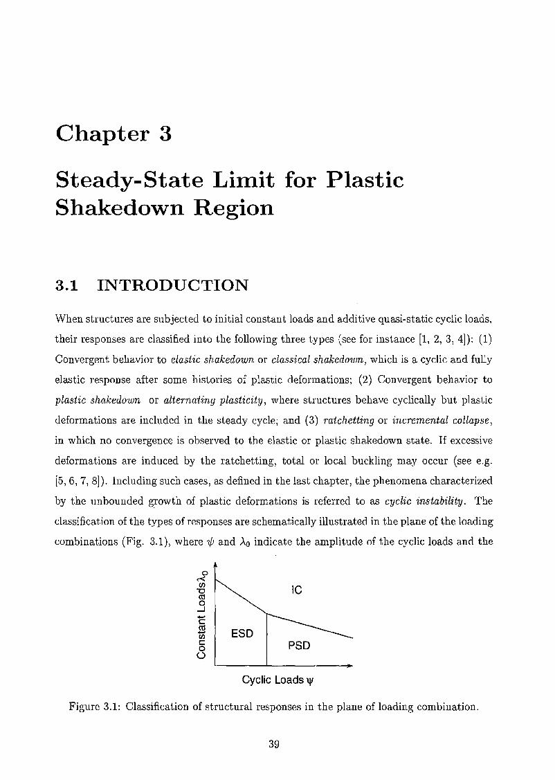
When structures are subjected to initial constant loads and additive quasi-static cyclic loads,
their responses are classified into the following three types (see for instance [1, 2, 3, 4]): (1)
Convergent behavior to elastic shakedown or classical shakedown, which is a cyclic and fully
elastic response after some histories of plastic deformations; (2) Convergent behavior to
plastic shakedown or alternating plasticity, where structures behave cyclically but plastic
deformations are included in the steady cycle; and (3) mtchetting or incremental collapse,
in which no convergence is observed to the elastic or plastic shakedown state. If excessive
deformations are induced by the ratchetting, total or local buckling may occur (see e.g.
[5,6, 7, 8]). Including such cases, as defined in the last chapter, the phenomena characterized
by the unbounded g~owth of plastic deformations is referred to as cyclic instability. The
classification of the types of responses are schematically illustrated in the plane of the loading
combinations (Fig. 3.1), where 'IjJ and AD indicate the amplitude of the cyclic loads and the
~en
"0eelo
..J.....C
~c:o()
PSD
Cyclic Loads \jI
Figure 3.1: Classification of structural responses in the plane of loading combination.
39
magnitude of the constant loads, respectively. The regions in which the elastic shakedown
and the plastic shakedown take place are called respectively the elastic shakedown region
and the plastic shakedown region.
To design structures subjected to cyclic loads, one should obtain the boundary between
the shakedown regions and the region where cyclic instability occurs. For this purpose, a
number of studies have been conducted on the structural responses under cyclic loading. The
approaches employed in the studies are roughly classified in the following two categories: one
is to trace all loading histories and the other is to predict the boundary theoretically without
tracing the loading histories.
To investigate the elastoplastic responses and to bound convergence and divergence of
plastic deformations, a direct but elaborating approach is to trace all the loading histories of
the structures. Experimental, analytical, and numerical methods are available to this end [3].
By tracing all the loading histories, we can observe the process of deformations and bound
the loading conditions below which the structures behave in a stable manner. Nonetheless,
generally, analytical methods can be applied only to very simple models. And experimental
and numerical approaches require a number of parametric analyses to bound the structural
responses. Moreover, it is very difficult to derive theoretical conditions similar to the Euler
buckling load from the parametric analyses
To obtain the theoretical condition below which the elastic shakedown occurs, numer
ous papers have been published on the shakedown theory [I, 4]. The classical shakedown is
extended in several papers [9, 10, 11, 12] to derive the condition below which plastic shake
down occurs. But only a little research [5, 13] has been made to derive the conditions that
bounds the plastic shakedown and the cyclic instability taking the geometrical nonlineari
ty into account. Furthermore, the path-independent shakedown theories are not promising
when strong influence of geometrical nonlinearity exists because the responses are inherently
path-dependent in such cases.
To overcome these difficulties, the steady-state limit theory was proposed by Uetani [14,
15] for cantilever beam-columns. Under cyclic bending with stepwisely increasing amplitude
in the presence of a certain compressive axial force, a beam-column exhibits convergence to
steady states before the amplitude reaches a limit, and, after the limit, the beam-column
will no longer exhibit any convergence. This limit is called the steady-state limit [7, 14].
With the steady-state limit theory, though under a specified loading history, the steady
state limit can be predicted as a theoretical critical point even if the strong effect of the
geometrical nonlinearity exist. In the previous chapter, based on the steady-state limit
40

theory for cantilever beam-columns, a method has been presented for finding the steady
state limit of trusses that bounds the elastic shakedown and the cyclic instability. But
several cases have been observed in which the method fail to find the steady-state limit that
bounds plastic shakedown and cyclic instability.
The purpose of this chapter is to present a method for predicting the steady-state limit for
the plastic shakedown region. For brevity, the method presented in the previous chapter is
simply called the previous method throughout this chapter. In this chapter, first, properties
of the structural responses with the plastic shakedown are studied to clarify the reason
why the previous method fail to find the steady-state limit when the plastic shakedown
takes place. In the study, our attention is focused on the validity of the hypothesis on
strain reversals employed in the previous method. Then, on the basis of the reason made
clear, the hypothesis on strain reversals is extended and fundamental concepts are outlined.
Second, incremental relations for variation of a steady state are formulated with respect to
the variation of the amplitude of the cyclic loads. Finally, validity of the proposed method
is demonstrated through numerical examples.
3.2 GOVERNING EQUATIONS
3.2.1 Analytical Model
Consider pin-jointed space trusses with M elements and N nodes. Buckling of the element is
ruled out but that of a global type is taken into account using the Total Lagrangian formu
lation. Under the assumption of large displacement-small strain, compatibility conditions
Figure 3.2: A truss element.
41
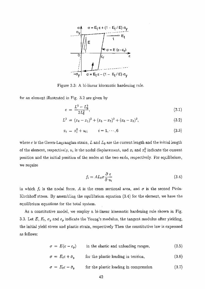
0,,III
rIII
cr =Et € + (1 - Et I E) cry----------_.
-~==E1 t
.... ------_ ... ---
-cry cr = Et E - (1 - Et I E) cry
Figure 3.3: A hi-linear kinematic hardening rule.
for an element illustrated in Fig. 3.2 are given by
2£5
(X4 - xd2+ (X5 - X2? + (X6 - X3?'
(3.1)
(3.2)
(3.3)
where c is the Green-Lagrangian strain, Land L o are the current length and the initial length
of the element, respectively, Ui is the nodal displacement, and Xi and x? indicate the current
position and the initial position of the nodes at the two ends, respectively. For equilibrium,
we require
(3.4)
in which Ii is the nodal force, A is the cross sectional area, and (f is the second Piola
Kirchhoff stress. By assembling the equilibrium equation (3.4) for the element, we have the
equilibrium equations for the total system.
As a constitutive model, we employ a bi-linear kinematic hardening rule shown in Fig.
3.3. Let E, Et , (fy and cp indicate the Young's modulus, the tangent modulus after yielding,
the initial yield stress and plastic strain, respectively Then the constitutive law is expressed
as follows:
in the elastic and unloading ranges,
for the plastic loading in tension,
for the plastic loading in compression
42
(3.5)
(3.6)
(3.7)
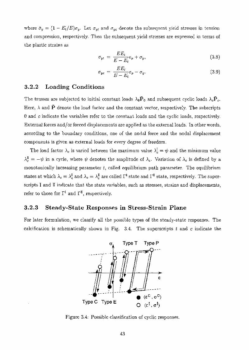
where ily = (1 - EtlE)ay. Let (Jyt and (Jyc denote the subsequent yield stresses in tension
and compression, respectively. Then the subsequent yield stresses are expressed in terms of
the plastic strains as
(3.8)
(3.9)
3.2.2 Loading Conditions
The trusses are subjected to initial constant loads )"oI>o and subsequent cyclic loads )"cI>c'
Here, )" and I> denote the load factor and the constant vector, respectively. The subscripts
o and c indicate the variables refer to the constant loads and the cyclic loads, respectively.
External forces and/or forced displacements are applied as the external loads. In other words,
according to the boundary conditions, one of the nodal force and the nodal displacement
components is given as external loads for every degree of freedom.
The load factor Ac is varied between the maximum value A~ = 1/J and the minimum value
),,~ = -7jJ in a cycle, where 1/) denotes the amplitude of )"c' Variation of Ac is defined by a
monotonically increasing parameter t, called equilibrium path parameter. The equilibrium
states at which Ac = ),,~ and )"C = A~ are called r l state and rn state, respectively. The super
scripts I and II indicate that the state variables, such as stresses, strains and displacements,
refer to those for r I and r n, respectively.
3.2.3 Steady-State Responses in Stress-Strain Plane
For later formulation, we classify all the possible types of the steady-state responses. The
calcification is schematically shown in Fig. 3.4. The superscripts t and c indicate the
cr Type T Type P
Type C Type E• (£c, crc)
o (£t, crt)
Figure 3.4: Possible classification of cyclic responses.
43
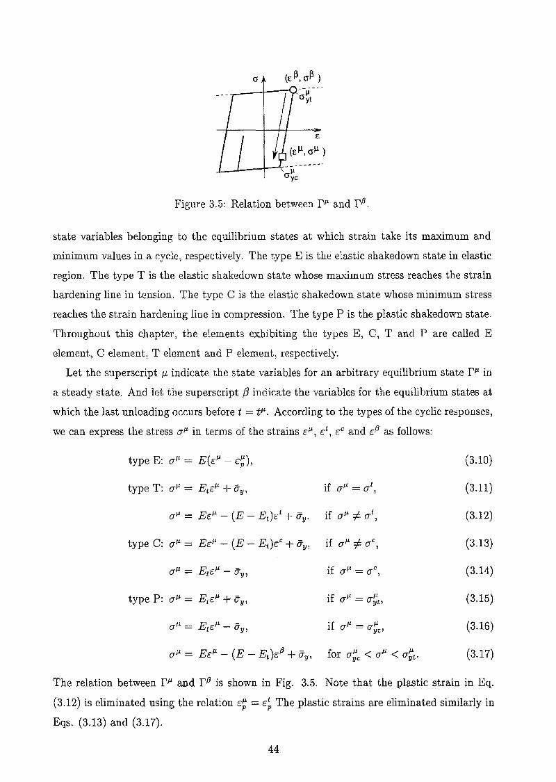
(£~, a~ )~ _... - _.
----+--~ allyt
Figure 3.5: Relation between f!" and fP.
state variables belonging to the equilibrium states at which strain take its maximum and
minimum values in a cycle, respectively. The type E is the elastic shakedown state in elastic
region. The type T is the elastic shakedown state whose maximum stress reaches the strain
hardening line in tension. The type C is the elastic shakedown state whose minimum stress
reaches the strain hardening line in compression. The type P is the plastic shakedown state.
Throughout this chapter, the elements exhibiting the types E, C, T and P are called E
element, C element, T element and P element, respectively.
Let the superscript /.L indicate the state variables for an arbitrary equilibrium state f/l in
a steady state. And let the superscript f3 indicate the variables for the equilibrium states at
which the last unloading occurs before t = tJ..!. According to the types of the cyclic responses,
we can express the stress (7/l in terms of the strains E/l, Et , c: C and E;f3 as fol1O'\:\'s:
type E: (JJ..! = E(c:/l - E~), (3.10)
type T: (7J..! = Etc:J..! + o-y, if (7/l = (7t (3.11),
(7J..! = EeJ..! - (E - Et)c:t + iJ"y, if (7J..! =f:. (7 t , (3,12)
type C: (7J..! = Ec:J..! - (E - Et)cC + iJ"y, if (7/l =f:. (7C 1 (3.13)
(7J..! = E J..! - if (JJ~ = (Jc, (3.14)tf: - (Jy,
type P: (J/l = Etc:/l + o-y, if (71' = (7J..! (3.15)yt,
(71' = E /l - 'f /l - /l (3.16)tC - (Jy, 1 (7 - (7yc'
(J/l = Ec:J1. - (E - Et )c:{3 + o-y, for (7~c < (J/l < tJ~t. (3.17)
The relation between fJ1. and ffJ is shown in Fig. 3.5. Note that the plastic strain in Eq,
(3.12) is eliminated using the relation c:~ = c:~ The plastic strains are eliminated similarly in
Eqs. (3.13) and (3.17).
44
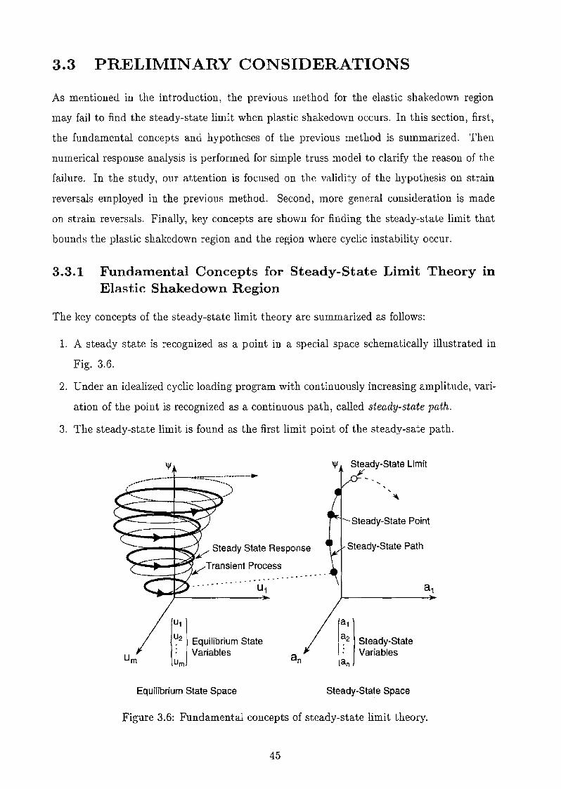
3.3 PRELIMINARY CONSIDERATIONS
As mentioned in the introduction, the previous method for the elastic shakedown region
may fail to find the steady-state limit when plastic shakedown occurs. In this section, first,
the fundamental concepts and hypotheses of the previous method is summarized. Then
numerical response analysis is performed for simple truss model to clarify the reason of the
failure. In the study, our attention is focused on the validity of the hypothesis on strain
reversals employed in the previous method. Second, more general consideration is made
on strain reversals. Finally, key concepts are shown for finding the steady-state limit that
bounds the plastic shakedown region and the region where cyclic instability occur.
3.3.1 Fundamental Concepts for Steady-State Limit Theory inElastic Shakedown Region
The key concepts of the steady-state limit theory are summarized as follows:
1. A steady state is recognized as a point in a special space schematically illustrated in
Fig. 3.6.
2. Under an idealized cyclic loading program with continuously increasing amplitude, vari
ation of the point is recognized as a continuous path, called steady-state path.
3. The steady-state limit is found as the first limit point of the steady-sate path.
Steady-State Point
Steady-State Path
'IV Steady-State Limit¥
~--~;;;:: y Steady State Response
,./Transient Process----:;;;;~~~
""'....--....--------'"""t-!!!'!-.~"- ...--__-:::::~~--- •.-,'
U1 a1
U2 Equilibrium State a2 Steady-State
UrnVariables an Variables
urn an
EqUilibrium State Space Steady-State Space
Figure 3.6: Fundamental concepts of steady-state limit theory.
45
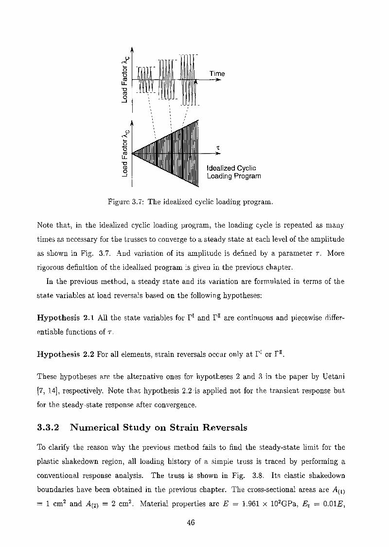
)-''-0
Time-()
ctI rLL ~"0ctl0
.....J ,,
'-ot5~"0ctIo
.....JIdealized CyclicLoading Program
Figure 3.7: The idealized cyclic loading program.
Note that, in the idealized cyclic loading program, the loading cycle is repeated as many
times as necessary for the trusses to converge to a steady state at each level of the amplitude
as shown in Fig. 3.7. And variation of its amplitude is defined by a parameter T. More
rigorous definition of the idealized program is given in the previous chapter.
In the previous method, a steady state and its variation are formulated in terms of the
state variables at load reversals based on the following hypotheses:
Hypothesis 2.1 All the state variables for r I and r IT are continuous and piecewise differ
entiable functions of T.
Hypothesis 2.2 For all elements, strain reversals occur only at r I or r IT •
These hypotheses are the alternative ones for hypotheses 2 and 3 in the paper by Uetani
[7, 14]' respectively. Note that hypothesis 2.2 is applied not for the transient response but
for the steady-state response after convergence.
3.3.2 Numerical Study on Strain Reversals
To clarify the reason why the previous method fails to find the steady-state limit for the
plastic shakedown region, all loading history of a simple truss is traced by performing a
conventional response analysis. The truss is shown in Fig. 3.8. Its elastic shakedown
boundaries have been obtained in the previous chapter. The cross-sectional areas are A(l)
= 1 cm2 and A(2) = 2 cm2. Material properties are E = 1.961 x 1Q2GPa, Et = O.OlE,
46

(ly = 2.942 x 10² MPa. The truss is subjected to the initial constant force >'oFo and the
additive forced displacement AcUc. Throughout all cycles, the amplitude 'l/J of the load factor
Ac is kept a constant value 1[J. The constants for the external loads are determined so that
the loading condition lies in the plastic shakedown region: if; = 0.13, Fo = 9.807 x 10³ N1
Uc = lcm and AO/ Ab = 0.375, where Ab = 0.7477 is the load factor at buckling in the sense
of Hill [16] when only the initial loads are applied.
100cm
Initial Force AoFoE
iJ100cm
Figure 3.8: The two-bar truss.
(X 10,3) (x 10,3)
1.0 1.0
I 0.5 I 0.5--U 0.0 --U 0.0.< .<
-0.5 ~0.5
-1.0 -1.0
-4 -2 0 2 (X 10'3) -4 -2 aE(1)
(a) Strain-Displacement Relations
1.0
0.5>.
\:)
~O.Ob
-0.5
-1.0
DYielding• Load Reversal 1.0
0.5>.
\:)
""1; 0.0b
-0.5
-1.0 /o-4 -2a-4 -2
£(1)
(b) Stress-Strain Relations
Figure 3.9: Strain-displacement relations and stress-strain relations.
47
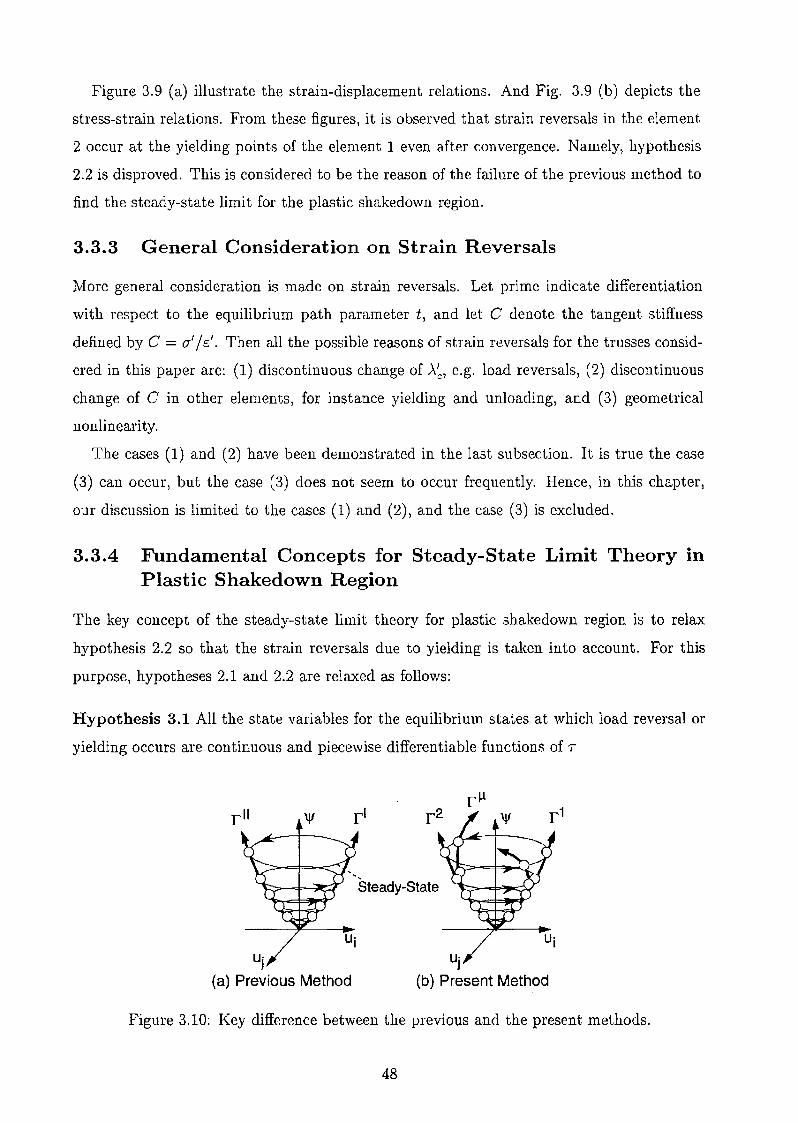
Figure 3.9 (a) illustrate the strain-displacement relations. And Fig. 3.9 (b) depicts the
stress-strain relations. From these figures, it is observed that strain reversals in the element
2 occur at the yielding points of the element 1 even after convergence. Namely, hypothesis
2.2 is disproved. This is considered to be the reason of the failure of the previous method to
find the steady-state limit for the plastic shakedown region.
3.3.3 General Consideration on Strain Reversals
More general consideration is made on strain reversals. Let prime indicate differentiation
with respect to the equilibrium path parameter t, and let C denote the tangent stiffness
defined by C = (// £'. Then all the possible reasons of strain reversals for the trusses consid
ered in this paper are: (1) discontinuous change of ..\~, e.g. load reversals, (2) discontinuous
change of C in other elements, for instance yielding and unloading, and (3) geometrical
nonlinearity.
The cases (1) and (2) have been demonstrated in the last subsection. It is true the case
(3) can occur, but the case (3) does not seem to occur frequently. Hence, in this chapter,
our discussion is limited to the cases (1) and (2), and the case (3) is excluded.
3.3.4 Fundamental Concepts for Steady-State Limit Theory inPlastic Shakedown Region
The key concept of the steady-state limit theory for plastic shakedown region is to relax
hypothesis 2.2 so that the strain reversals due to yielding is taken into account. For this
purpose, hypotheses 2.1 and 2.2 are relaxed as follows:
Hypothesis 3.1 All the state variables for the equilibrium states at which load reversal or
yielding occurs are continuous and piecewise differentiable functions of T
r l
u·Iu·J
(a) Previous Method
Steady-State
u·J(b) Present Method
Figure 3.10: Key difference between the previous and the present methods.
48
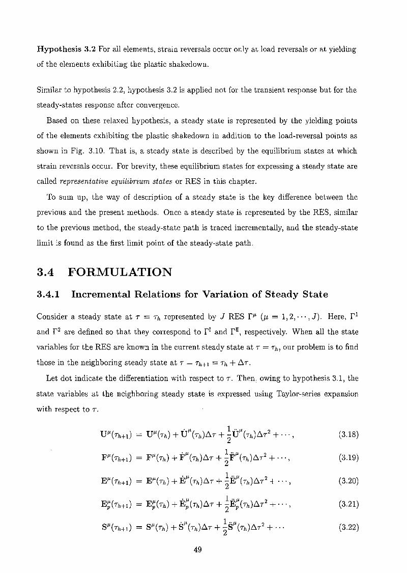
Hypothesis 3.2 For all elements, strain reversals occur only at load reversals or at yielding
of the elements exhibiting the plastic shakedown.
Similar to hypothesis 2.2, hypothesis 3.2 is applied not for the transient response but for the
steady-states response after convergence.
Based on these relaxed hypothesis, a steady state is represented by the yielding points
of the elements exhibiting the plastic shakedown in addition to the load-reversal points as
shown in Fig. 3.10. That is, a steady state is described by the equilibrium states at which
strain reversals occur. For brevity, these equilibrium states for expressing a steady state are
called representative equilibrium states or RES in this chapter.
To sum up, the way of description of a steady state is the key difference between the
previous and the present methods. Once a steady state is represented by the RES, similar
to the previous method, the steady-state path is traced incrementally, and the steady-state
limit is found as the first limit point of the steady-state path.
3.4 FORMULATION
3.4.1 Incremental Relations for Variation of Steady State
Consider a steady state at 7 = 7h represented by J RES r li (J.l = 1,2,"" J). Here, r 1
and r 2 are defined so that they correspond to r 1 and r lI , respectively. When all the state
variables for the RES are known in the current steady state at 7 = 7h, our problem is to find
those in the neighboring steady state at 7 = 7hH = Th + !J.7.
Let dot indicate the differentiation with respect to T. Then, owing to hypothesis 3.1, the
state variables at the neighboring steady state is expressed using Taylor-series expansion
with respect to T.
. Ii 1 .. Ii 2UJl(Th+l) = UJl(7h) + U (Th)!J.T + 2"U (7h)!J.T + ... ,
. J1. 1 "Ii 2FJ1.(7h+d = FJ1.(Th) + F (Th)!J.T + 2"F (Th)!J.7 +"',
'Jl 1"Jl 2EJl(Th+d = EIi(7h) + E (Th)!J.T + 2"E (Th)!J.T +''',
. J1. 1 OOI-L 2E~(Th+l) = E~(Th) + Ep (7h)!J.T + 2"Ep (7h)!J.T +"',
• I-L 1 "/J 2SJl(Th+l) = SJl(Th) + 8 (7h)!J.T + 2"8 (Th)!J.T +."
49
(3.18)
(3.19)
(3.20)
(3.21)
(3.22)
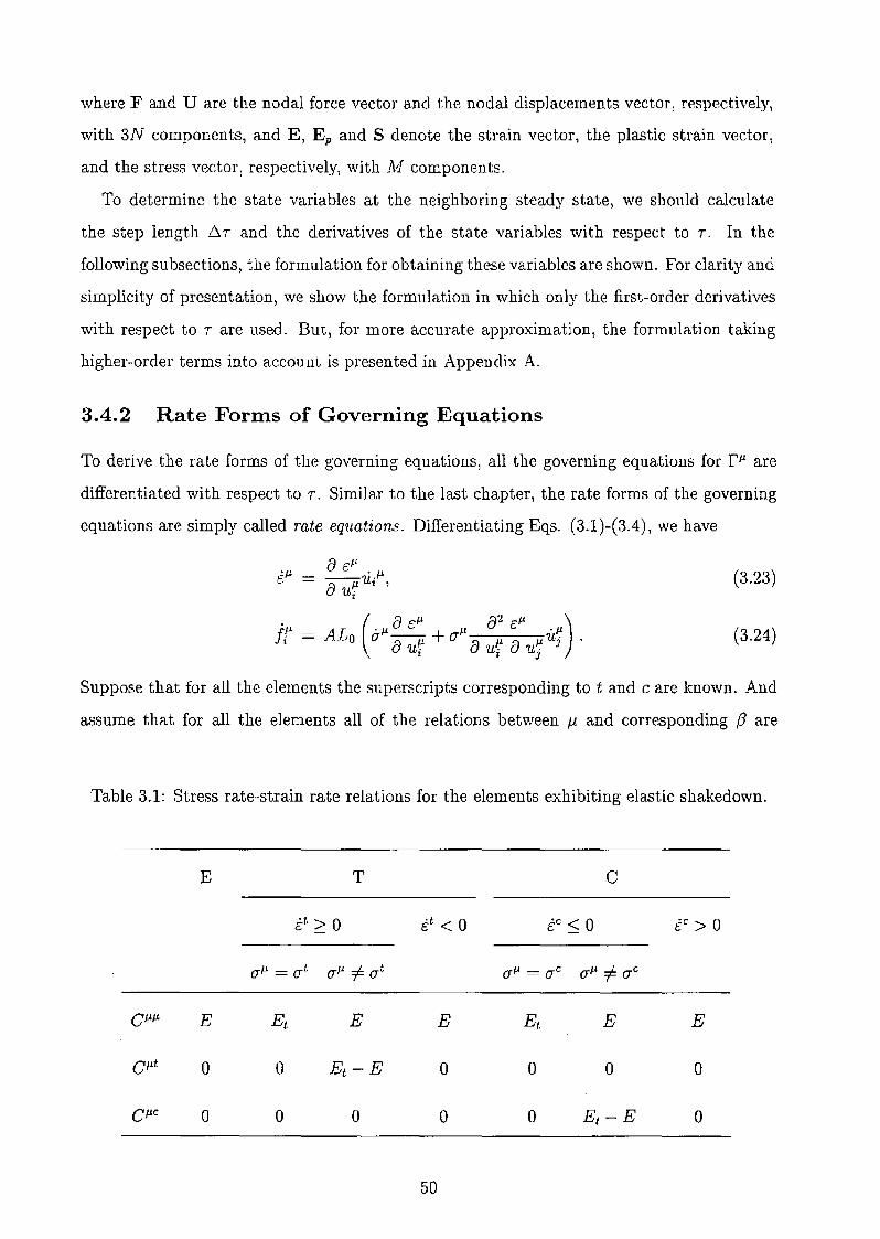
where F and U are the nodal force vector and the nodal displacements vector, respectively,
with 3N components, and E, E p and S denote the strain vector, the plastic strain vector,
and the stress vector, respectively, with !v! components.
To determine the state variables at the neighboring steady state, we should calculate
the step length t:.T and the derivatives of the state variables with respect to T. In the
following subsections, the formulation for obtaining these variables are shown. For clarity and
simplicity of presentation, we show the formulation in which only the first-order derivatives
with respect to T are used. But, for more accurate approximation, the formulation taking
higher-order terms into account is presented in Appendix A.
3.4.2 Rate Forms of Governing Equations
To derive the rate forms of the governing equations, all the governing equations for f/l are
differentiated with respect to T. Similar to the last chapter, the rate forms of the governing
equations are simply called rate equations. Differentiating Eqs. (3.1)-(3.4), we have
B Etl . tl~Ui ,u u·l
(3.23)
(3.24)
Suppose that for all the elements the superscripts corresponding to t and c are known. And
assume that for all the elements all of the relations between J-t and corresponding {3 are
Table 3.1: Stress rate-strain rate relations for the elements exhibiting elastic shakedown.
E T C
it 2: 0 it < 0 i C::; 0 i C > 0
(Jtl = (Jt (Jtl #:- at (JJl = (Jc (Jtl #:- aC
GtlJl E Et E E Et. E E
Gilt 0 0 Et-E 0 0 0 0
Cpc 0 0 0 0 0 Et-E 0
50

Table 3.2: Stress rate-strain rate relations for the elements exhibiting plastic shakedown.
E
o o Et-E
known. Differentiating Eqs. (3.10)-(3.13), we have the stress rate-strain rate relations for
the E, T and C elements. The rate relations are expressed as
(3.25)
where C/iJ1., CJ1.t and CJ1.C are the coefficients that are chosen according to Table 3.1. For the
P elements, differentiation of Eqs. (3.15)-(3.17) leads to
(3.26)
in which CJ1.J1. and C/i(3 are the coefficients that are selected according to Table 3.2. After
replacing the superscripts t, C and (3 with those indicating the corresponding RES, we can
express the rate forms of stress-strain relations
J
iJJ1. = L C/iV rY'v=l
(3.27)
where CJ1.V is the coefficient of the strain rates. Substituting Eqs. (3.23) and (3.27) into Eq.
(3.24), we have the rate equations for element
J
jr = L k:jitj,v=l
(3.28)
where oJ1.V is the Kronecker's delta and ktll is the coefficient relating jr and it}. By assembling
Eq. (3.28), the following rate equations are derived for the total system
'J-'F
where KJ1.V is coefficient matrix of If.
51
(3.29)

a
~_ ..... --_.
(€ 11, all )
Figure 3.11: [J' as an yielding point.
Now we have J x 3N equations that relates the rate vectors of the nodal forces and the
nodal displacements. On the other hand, there are J unknowns of :\1' in addition to J x 3N
unknown components of the rate vectors of the nodal forces and/or nodal displacements.
Namely, we have Jx (3N+1) unknowns. Consequently, additional J equations are apparently
needed to solve the rate equations.
Assume that for all the RES [J' (Jl ~ 3) the element whose yielding characterize fJl are
known. For the equilibrium states at load reversals, we have
. 2 • n ...\ =..\ = _nl,c c 'fI
(3.30)
(3.31)
which characterize the load reversals [1 and [ll. In contrast, the equilibrium states fJl (Jl ~ 3)
are characterized as the yielding point of the element exhibiting the plastic shakedown.
Consider the case [Jl is characterized as the equilibrium state at which compressive yielding
occurs as shown in Fig. 3.11. At the yielding point of the element whose yielding defines
[Jl , both Eqs. (3.15) and (3.17) are satisfied. Hence we have
(3.32)
Differentiation of Eq. (3.32) yields the rate relation
(3.33)
The condition (3.33) is expressed in terms of the nodal displacements for the element as
(3.34)
52
The condition Eq. (3.34) can be rewritten in terms of the nodal displacement for the total
system as
(3.35)
where L is the coefficient matrix of U, and 0 is zero vector. The conditions that characterize
the yielding in tension is derived similarly and is expressed in the same form of Eq. (3.35).
After replacing the superscript (3 to that for the corresponding RES, we have J - 2 equations
in addition to Eqs. (3.30) and (3.31). Thus we have the same number of the equations as
that of the unknowns. These equations are to be solved by specifying the value of 7/J and by
using the boundary conditions.
3.4.3 Consistent Set of Stress Rate-Strain Rate Relations
If an element exhibits type T or type C behavior, the coefficients of the strain rates should
be chosen according to the signs of the strain rates as shown in Table 3.1. Therefore, for all
the elements exhibiting the type T or the type C behavior, we should choose a set of the
coefficients that are consistent with the signs of the resulting strain rates.
To find the consistent set of the coefficients, we employ a trial and error approach, which
is also used in the conventional response analysis [17]. In the trial and error approach, first,
the signs of the strain rates F/' are assumed to be equal to those in the last step. Then,
the coefficients CI'I', Cl't and CI-lC are determined according to the assumptions, and the
rate equations are constructed. After the rate equations are solved and EI-l are calculated,
the consistency is checked between the assumed signs of the strain rates and the resulting
ones for all the elements exhibiting the type T or the type C behavior. If the signs are not
consistent, the assumed signs are reversed. This procedure is continued until all the resulting
signs of the strain rates are consistent with the assumed ones.
3.4.4 Termination Conditions for Incremental Steps
Different stress rate-strain rate relations should be employed in Eq. (3.27) for the steady
states at T 2: Th+l when the types of stress-strain cyclic responses, the order of the RES
or the number of the RES may change at T = Th+!. In such cases, an incremental step
is terminated at T = Th+l. The conditions for terminating the incremental steps are given
by the following equations. The step length I:i.T is determined as the smallest value among
l:i.tmax , specified for preventing excessive accumulation of truncation errors, and the values
obtained from these conditions.
53

First, consider the transition of the types of the cyclic responses. For E elements, 6..T is
calculated using the following conditions:
(3.36)
(3.37)
where the subsequent yield stresses are expressed in terms of Ep(Th) using Eqs. (3.8) and
(3.9), and a(Th+d is expressed as a(Th) + &(Th)6..T in the linear approximation. Equations
(3.36) and (3.37) are the conditions for E -+ T and E -+ C, respectively. For every E, T and
C element, the condition for the transition to the type P is written as
(3.38)
An example of the transition is shown in Fig. 3.12 (a).
Next, let us discuss the change of the order or the number of the RES. Let the superscripts
a: and a: + 1 indicate the stresses at two consecutive instants in a cycle. Then the condition
for the change of the order of the RES is written by
The condition for increasing the number of the RES are given by
(3.39)
if (Jf3 = (Jf3 at T = T}yc 1, (3.40)
(3.41)
Note that, obviously, the number of the RES should be increased when the transition E, T
or C -+ P occurs.
3.4.5 Examination of Strain Reversals
In constructing the rate equations and in determining the incremental steps, the following
things are assumed to be known: (1) the element whose yielding characterize flj (Il- ;::: 3); (2)
the equilibrium states corresponding to r t and rc for all the elements; and (3) the relations
between J.L and corresponding f3 for all the P elements. These relations may change if the
order or the number of the RES changes. In the previous section, the conditions (3.38)-(3.41)
have been given for terminating incremental steps at these instants. If the incremental steps
are terminated using at least one of these conditions, it must be examined whether the
relations (1)-(3) change or not. For this purpose, we examine strain reversals.
54
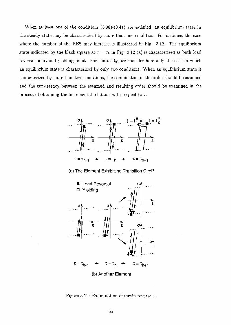
When at least one of the conditions (3.38)-(3.41) are satisfied) an equilibrium state in
the steady state may be characterized by more than one condition. For instance, the case
where the number of the RES may increase is illustrated in Fig. 3.12. The equilibrium
state indicated by the black square at T = Tft in Fig. 3.12 (a) is characterized as both load
reversal point and yielding point. For simplicity, we consider here only the case in which
an equilibrium state is characterized by only two conditions. When an equilibrium state is
characterized by more than two conditions) the combination of the order should be assumed
and the consistency between the assumed and resulting order should be examined in the
process of obtaining the incremental relations with respect to T.
(j
E
cr
---~ ----
(a) The Element Exhibitting Transition C ..p
• Load Reversalo Yielding
(j
-----
----
(j
(j
-~--
E (j-----
(b) Another Element
Figure 3.12: Examination of strain reversals.
55
Let pI be characterized by two conditions at T = Th. First, to examine the strain reversals,
the order of the equilibrium states are determined in the steady state for T > Th. If the
number of the RES may increase, the new yielding is considered to occur preceding Pi. An
example is shown in Fig. 3.12, where the black square indicate the load reversal point fll
and the white square indicate the new yielding point. On the other hand, if the order of the
RES in a steady state is changed, the order in the steady state for T < Til is reversed.
Second, it is checked whether or not strain reversals occur at the two equilibrium states
in the steady state for T > Th. For this purpose, the partial derivatives with respect to t is
used. Let tf. and t~ (ti ::; t~) denote respectively the instants for the equilibrium states in a
steady sate at T > Th as shown in Fig. 3.12. A strain reversal is judged to occur at t = tf if
the following condition
8e:1- Be: +- x- <08 t t=t-i 8 t t"",ti
(3.42)
is satisfied. Otherwise, no stain reversal is judged to take place. The condition for t = t~ is
written in the same form as Eq. (3.42). These conditions are checked for every the element.
The procedures for calculating the partial derivatives are shown in Appendix B.
Finally, if the strain reversals are judged to occur in at least one element at the time
where no strain reversal occurs in the steady state for T < Th, the yielding point is added to
the RES. And according to the result of the examination of the strain reversals, the relations
(1)-(3) are changed if changes aTe needed.
3.4.6 Steady-State Limit Condition
Now, all the first-order derivatives and the step length 67 have been obtained. Substituting
67 and the first-order derivatives into Eq. (3.18) we have all the state variables at T = Th+1'
Repeating these procedures, the steady-state path is traced incrementally.
As mentioned before, the steady-state limit is characterized as the first limit point of the
steady-state path. The steady-state limit condition is therefore given as
(3.43)
Note that, to find the limit point and to trace the steady-state path after the limit point, a
procedure should be employed similar to displacement control schemes [17, 18].
56
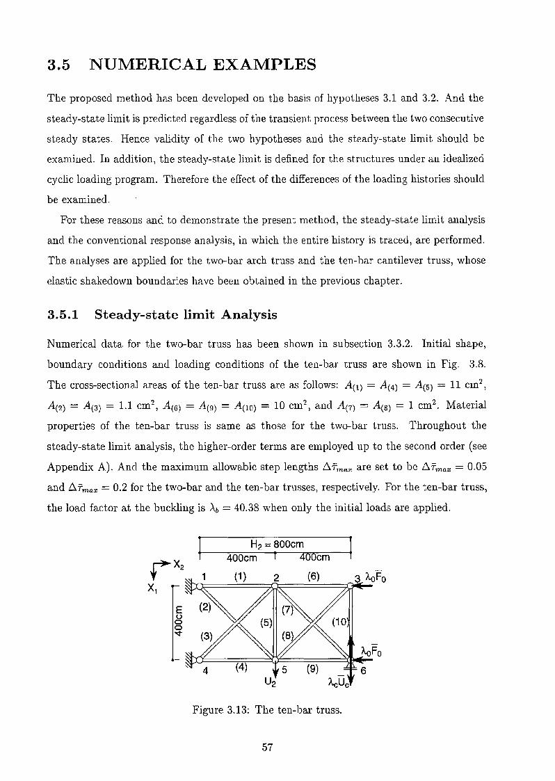
3.5 NUMERICAL EXAMPLES
The proposed method has been developed on the basis of hypotheses 3.1 and 3.2. And the
steady-state limit is predicted regardless of the transient process between the two consecutive
steady states. Hence validity of the two hypotheses and the steady-state limit should be
examined. In addition, the steady-state limit is defined for the structures under an idealized
cyclic loading program. Therefore the effect of the differences of the loading histories should
be examined.
For these reasons and to demonstrate the present method, the steady-state limit analysis
and the conventional response analysis, in which the entire history is traced, are performed.
The analyses are applied for the two-bar arch truss and the ten-bar cantilever truss, whose
elastic shakedown boundaries have been obtained in the previous chapter.
3.5.1 Steady-state limit Analysis
Numerical data for the two-bar truss has been shown in subsection 3.3.2. Initial shape,
boundary conditions and loading conditions of the ten-bar truss are shown in Fig. 3.8.
The cross-sectional areas of the ten-bar truss are as follows: A(l) = A(4) = A(5) = 11 cm2,
A(2) = A(3) = 1.1 cm2, A(6) = A(9) = A{1o) = 10 cm2
, and A(i) = A(8) = 1 cm2. Material
properties of the ten-bar truss is same as those for the two-bar truss. Throughout the
steady-state limit analysis, the higher-order terms are employed up to the second order (see
Appendix A). And the maximum allowable step lengths D..fmax are set to be D..fmax = 0.05
and 6.fmax = 0.2 for the two-bar and the ten-bar trusses, respectively. For the ten-bar truss,
the load factor at the buckling is Ab = 40.38 when only the initial loads are applied.
H2 = 800em
Euoo
-.::t
400cm i 400em
AoFo
6
Figure 3.13: The ten-bar truss.
57
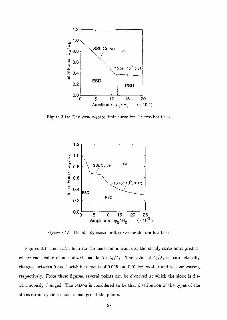
1.2 r------...---r----...,.------,
PSDESD
c4(15.09 x 10 .0.37)
I
1.0..0
«)0.8
CD~ 0.6oLL
ctS 0.4Ec
0.2
SSL Curve
/CI
20(x 104)
5 10 15Amplitude: 'Jf1 I H1
0.0 '--------'------"----"----'----'o
Figure 3.14: The steady-state limit curve for the two-bar truss.
1.2
~ 1.0-0 SSL Curve CI« 0.8/C1>
u0.6 !....
0 ILL 1 -3
ctSI (16.45 x 10 .0.37)I /:E 0.4 I
c ESOII
PSO!0.2 iI
I5 10 15
Amplitude: 'Jf2! ~
Figure 3.15: The steady-state limit curve for the ten-bar truss.
Figures 3.14 and 3.15 illustrate the load combinations at the steady-state limit predict
ed for each value of normalized load factor Ao/Ab. The value of Ao/Ab is parametrically
changed between 0 and 1 with increments of 0.005 and 0.01 for two-bar and ten-bar trusses,
respectively. From these figures l several points can be observed at which the slope is dis
continuously changed. The reason is considered to be that distribution of the types of the
stress-strain cyclic responses changes at the points.
58
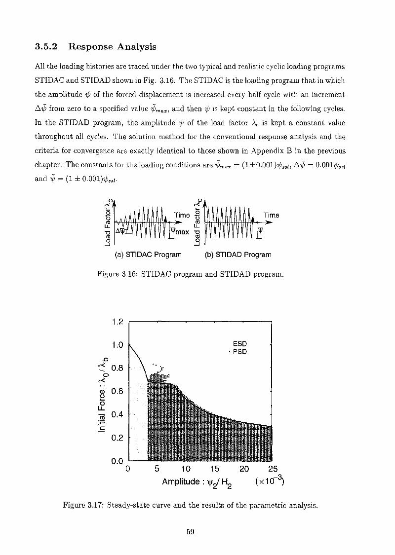
3.5.2 Response Analysis
All the loading histories are traced under the two typical and realistic cyclic loading programs
STIDAC and STIDAD shown in Fig. 3.16. The STIDAC is the loading program that in which
the amplitude 1/J of the forced displacement is increased every half cycle with an increment
6'¢ from zero to a specified value '¢max, and then 1/J is kept constant in the following cycles.
In the STIDAD program, the amplitude 'Ij; of the load factor Ac is kept a constant value
throughout all cycles. The solution method for the conventional response analysis and the
criteria for convergence are exactly identical to those shown in Appendix B in the previous
chapter. The constants for the loading conditions are '¢max = (1 ±O.OOl)1/Jssl, 6'¢ = O.OOl1/Jssl
and '¢ = (1 ± O.OOl)'l,bssl.
(a) STIDAC Program (b) STIDAD Program
Figure 3.16: STIDAC program and STIDAD program.
1.2
1.0
.cc<__ 0.8
oc<
(1) 0.62ou..C13 0.4Ec
0.2
0.0o
ESD. PSD
5 10 15
Amplitude: 'Vi H2
Figure 3.17: Steady-state curve and the results of the parametric analysis.
59

Under the STIDAC program, good agreement is observed between the the steady-state
limit predicted by the proposed method and the results of the response analysis. Convergence
is observed if '¢max < Wss/, and divergence is obtained if i/Jmax > 'l/Jss/' From this result, it
may be stated that the proposed method is directly verified. On the other hand, inconsistent
results are seen for the ten-bar truss under STIDAD program. Convergence is observed
regardless of if; > 'l/Jss/'
To clarify when this inconsistency occurs, a complete parametric analysis is carried out.
In the parametric analysis, not only AO but also if; are changed. The load factor AO of
the constant load is changed in the same manner as the steady-state limit analysis. The
constant amplitude of the cyclic forced displacement is changed from -/iJ/H2(x-3) = 0 to 25
with an increment of 0.25. Namely, the response analysis is performed for 10,000 different
load combinations of (Ao, -/iJ).
The results of the complete parametric analyses is illustrated in Fig. 3.17. When conver
gence is observed, the load combinations are plotted by the circular symbols. The darker
and lighter grey circles indicate the convergence to the plastic shakedown and the elastic
shakedown, respectively. From Fig. 3.17, we may state that the values of the steady-state
limit predicted under the idealized cyclic loading program may be smaller than the limiting
values that bound convergence and divergence predicted under the STIDAD program.
3.6 CONCLUSIONS
For elastoplastic trusses subjected to the cyclic loads in the presence of the constant loads,
a new method has been presented for finding the critical load combinations that bounds
convergence to plastic shakedown and divergence of plastic deformations.
The conclusions of this research are:
1. The reason has been clarified why the method presented in the previous chapter fails to
find the steady-state limit when plastic shakedown occurs. When an element exhibits
the plastic shakedown, strain reversals of the other elements may take place not only
at load reversals but also at yielding of the elements exhibiting the plastic shakedown.
Nevertheless it was assumed that the strain reversals occur only at the load reversals in
the previous method.
2. The hypothesis on the strain reversals has been relaxed so that the strain reversals
due to yielding is taken into account. Based on the relaxed assumption, incremental
relations have been formulated for tracing the variation of the steady state with respect
to the parameter that defined the amplitude of the cyclic loads.
60
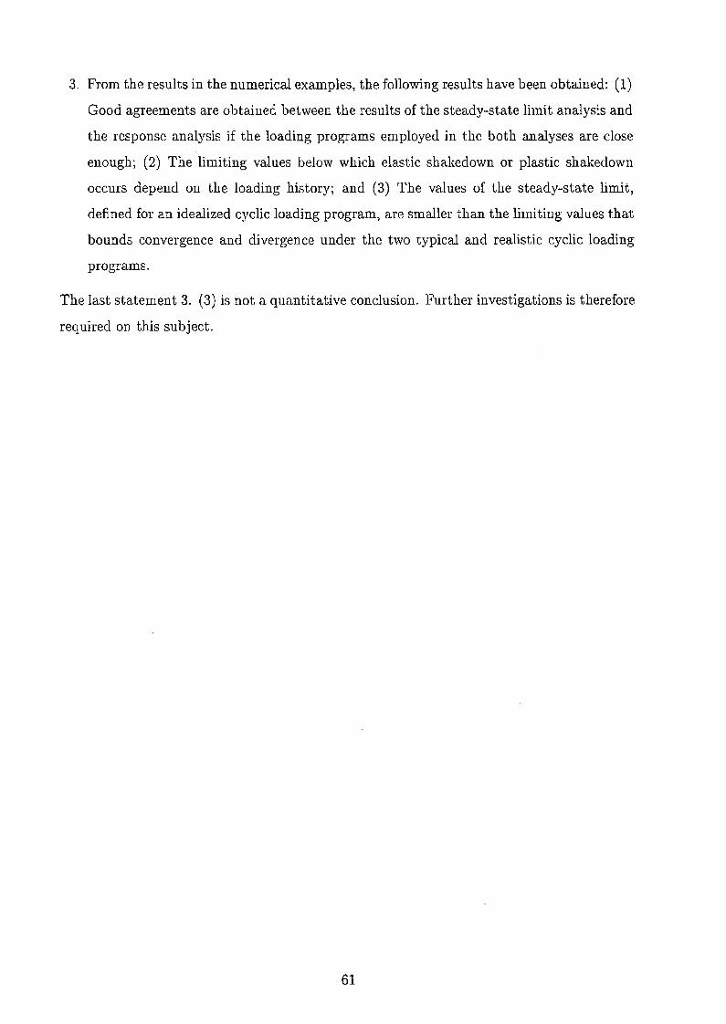
3. From the results in the numerical examples, the following results have been obtained: (1)
Good agreements are obtained between the results of the steady-state limit analysis and
the response analysis if the loading programs employed in the both analyses are close
enough; (2) The limiting values below which elastic shakedown or plastic shakedown
occurs depend on the loading history; and (3) The values of the steady-state limit,
defined for an idealized cyclic loading program, are smaller than the limiting values that
bounds convergence and divergence under the two typical and realistic cyclic loading
programs.
The last statement 3. (3) is not a quantitative conclusion. Further investigations is therefore
required on this subject.
61

Appendix A. Formulation with Higher-Order Derivatives
A formulation with higher-order derivatives is presented for the steady-state limit analysis.
We derive here the derivatives up to only the second order. But more higher-order derivatives
can be obtained similarly.
Differentiation of the rate equations (3.23)-(3.34) with respect to the steady-state path
parameter T yields the second-order perturbation equations as follows:
"p. 8 cJ.l "J.l 82cp. • p. ,/1
C = ~-U' + Uj Uj (3.44)8 ul·1I- I 8 u·1I- 8 u·p.
t J
for the compatibility conditions,
{8 p. 82
J.l 82p. }
f"l1- - AL "J.l C J1 C "II- 2'J1 C 'J.l. - 00"--+0" u·+ 0" u·t 8 uf 8 u j J1 8 u/ J 8 u j J1 8 Ujp. J
for the equilibrium conditions, and
JuJ1 = L cp.vEI/
1/=1
(3.45)
(3.46)
for the stress-strain relations. Note that GJ1J1 = 0 because the piecewise-linear constitutive
relation is assumed. Differentiating Eq. (3.28), we have the second-order perturbation
equations for each element
J
ff ~ kf:l~"~ + fA!,• - L...J lJ uJ t ,
1/=1
(3.47)
(3.48)
where the coefficients kfj is identical to that in Eq. (3.29) and hat indicates the variables
expressed in terms of the first-order derivatives as follows
82 p. 8 II- J 82 V
fAp. _ 2AL . p. C . p. AL _c_ ~ C"'''' c , v . vj - 00" 8 8 Uj + 0 8 J1 L...J 8 8 ujuk ·
U j J1 ujJ.l Uj v=1 Ujl/ 'Uk1/
Assembling the perturbation equations for the elements leads to the second-order perturba
tion equations for the total system
(3.49)
where the coefficient matrices are same as those in the rate equation (3.29). Differentiation
of Eqs. (3.30), (3.31) and (3.34) leads to
(3.50)
62
= 0,
=0
(3.51)
(3.52)
where
(3.53)
Equation (3.53) can be expressed in terms of nodal displacements for the total system as
(3.54)
By specifying the value of;j;, we have J x (3N + 1) simultaneous linear equations (3.49) and
(3.54).
When the derivatives are employed up to the second order, the termination conditions
Eqs. (3.36)-(3.38) of the incremental step become quadratic equations of the step length 6.7,
while the conditions are linear equations when only the first derivatives are used. Besides
these termination conditions, we must consider the conditions
(3.55)
(3.56)
for the transitions T ---+ E and C ---+ E, respectively.
Appendix B. Formulation for Examination of StrainReversals
A formulation is shown here for examining the strain reversals. Differentiating the kine
matic relations (3.1)-(3.3) with respect to t, we obtain the following equations
(3.57)
where the prime indicates partial differentiation with respect to t. Differentiation of equilib
rium condition (3.4) yields
(3.58)
These equations (3.57) and (3.58) are used for both t = tt and t = t~.
On the other hand, the constitutive relations may be different for the two instants. Con
sider first the case where t = ti. Define ct and C1 by
8c+Cf.£+ -1 --
8 (J t=t.i '
63
(3.59)
Then these coefficients Cr+ and Cr- are determined according to the type of the stress-strain
cyclic response. For the E, T and C elements, these coefficients are given by
(3.60)
because these elements exhibit elastic shakedown responses in the neighboring steady state
for T ~ Th. Recall that only the steady-state responses after convergence is considered in
the steady-state limit theory. For P elements, the coefficients are selected according to the
location of state point in the stress-strain plane. For the element whose yielding occurs at
t = tr, the coefficients are given by
(3.61)
For the element whose yielding occurs at t = t~, the coefficients are determined by
For the other elements, the coefficients are given by
(3.62)
Cfl+-E1 - t;
Cfl+ -E1 - ,
if (J'fl = (J'fl or (J'fl = (J'flyt yc (3.63)
(3.64)
Note that consistency between the assumed and resulting sign of £' must be checked when
the tangent stiffness Et is used.
Substitution of the coefficients Cr- and Cr+ into Eq. (3.58) and assemblage of the tangent
stiffness equations for elements lead to that for total system
F fl-' - Kfl-Ufl-' F fl+' - Kfl+Ufl+'1-1 1'1-11 (3.65)
By using the boundary conditions and by specifying )..~-' and )..~+', we can solve Eq. (3.65).
With strain-displacement relations, we have Er-' and Er+'·
Let us turn to the case where t = t~. Here, we have
E~-' = Ei+'. (3.66)
Our problem is then to calculate Ei+'. The only difference between the case for obtaining
Er+' and E~+' is the way to choose tangent stiffnesses. For the element whose yielding
occurs at t = ti, the coefficients are determined by
C'l+ - E2 - t· (3.67)
For the other elements, the coefficients C~+ are determined so that those are identical to
Cr+ after the consistent set of tangent stiffness is obtained. Note that, if unloading at t = tiand strain reversal t = t~ occur in an element, the element will yield at the time t > t~. The
strain reversals at the yielding time should be checked in a similar manner as that at t = ti.
64
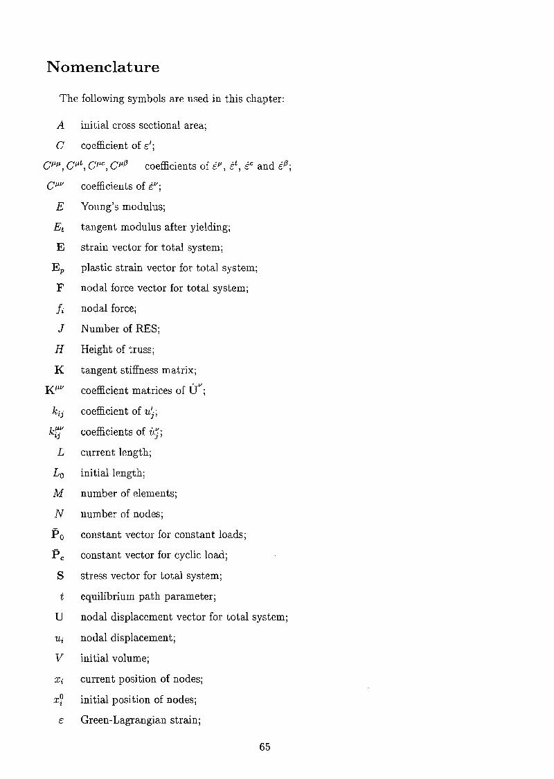
Nomenclature
The following symbols are used in this chapter:
A initial cross sectional area;
C coefficient of c:';
Cf.Jf.J Cf.J t Cf.Je Cf.Jf3 coefficients of if.J .;.t i C and i f3 ·J ~ , ) (.. , ,
E Young's modulus;
E t tangent modulus after yielding;
E strain vector for total system;
E p plastic strain vector for total system;
F nodal force vector for total system;
Ii nodal force;
J Number of RES;
H Height of truss;
K tangent stiffness matrix;
Kf.JV coefficient matrices of "it;
kij coefficient of uj;
krj coefficients of it};
L current length;
Lo initial length;
M number of elements;
N number of nodes;
Po constant vector for constant loads;
Pc constant vector for cyclic load;
S stress vector for total system;
t equilibrium path parameter;
U nodal displacement vector for total system;
Ui nodal displacement;
V initial volume;
Xi current position of nodes;
x? initial position of nodes;
c: Green-Lagrangian strain;
65
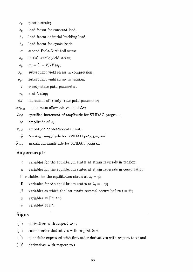
Ep plastic strain;
AO load factor for constant load;
Ab load factor at initial buckling load;
Ac load factor for cyclic loads;
CJ second Piola-Kirchhoff stress;
CJy initial tensile yield stress;
fly fly = (1 - EdE)CJy;
CJyc subsequent yield stress in compression;
CJyt subsequent yield stress in tension;
7 steady-state path parameter;
Ih 7 at h step;
1:11 increment of steady-state path parameter;
I:1fmax maximum allowable value of 1:17;
t:.7[J specified increment of amplitude for STIDAC program;
'ljJ amplitude of Ac ;
'l/Jssl amplitude at steady-state limit;
7[J constant amplitude for STIDAD program; and
7[Jmax maximum amplitude for STIDAC program.
Superscripts
t variables for the equilibrium states at strain reversals in tension;
c variables for the equilibrium states at strain reversals in compression;
I variables for the equilibrium states at Ac = W;
n variables for the equilibrium states at Ac = -'ljJ;
j3 variables at which the last strain reversal occurs before t = tP ;
tL variables at fP; and
v variables at P' ..
Signs
() derivatives with respect to I;
() second order derivatives with respect to I;
(~) quantities expressed with first-order derivatives with respect to 7; and
()' derivatives with respect to t.
66

References
[1] W. T. Koiter. General theorems for elastic-plastic structures. In J. N. Sneddon and
R. Hill, editors, Progress in Solid Mechanics, volume 1, pages 167-221, North Holland,
Amsterdam, 1960.
[2] J. Bree. Elastic-plastic behavior of thin tubes subjected to internal pressure and inter
mittent high-heat fluxes with application to fast-nuclear-reactor fuel elements. Journal
of Strain Analysis, 6:236-249, 1967.
[3] J. Zarka and J. Casier. Elastic-plastic response of a structure to cyclic loading: Practical
rules. In S. Nemat-Nasser, editor, Mechanics Today, pages 93-198. Pergamon Press, New
York, 1979.
[4] J. A. Konig. Shakedown of Elastic-Plastic Structures. Elsevier, Amsterdam, 1987.
[5] Q. S. Nguyen, G. Gary, and G. Baylac. Interaction buckling-progressive deformation.
Nuclear Engineering and Design, 75:235-243, 1983.
[6] A. Siemaszko and J. A. Konig. Analysis of stability of incremental collapse of skeletal
structures. Journal of Structural Mechanics, 13:301-321, 1985.
[7] K. Uetani and T. Nakamura. Symmetry limit theory for cantilever beam-columns sub
jected to cyclic reversed bending. Journal of the Mechanics and Physics of Solids,
31(6):449-484, 1983.
[8] G. Maier, L. G. Pan, and U. Perego. Geometric effects on shakedown and ratchetting
of axisymmetric cylindrical shells subjected to variable thermal loading. Engineering
Structures, 15:453-465, 1993.
[9] A. R. S. Ponter and S. Karadeniz. An extended shakedown theory for structures that
suffer cyclic thermal loadings, part 1: Theory. Journal of Applied Mechanics, 52:877
882, 1985.
[10] A. R. S. Panter and S. Karadeniz. An extended shakedown theory for structures that
suffer cyclic thermal loadings, part 2: Applications. Journal of Applied Mechanics,
52:883-889, 1985.
[11] C. Polizzotto. A study on plastic shakedown of structures, part i: Basic properties.
Journal of Applied Mechanics, 60:318-323, 1993.
[12] C. Polizzotto. A study on plastic shakedown of structures, part ii: Theorems. Journal
of Applied Mechanics, 60:324-330, 1993.
67
[13] C. Polizzotto and G. Borio. Shakedown and steady-state responses of elastic-plastic
solids in large displacements. International Journal of Solids and Structures, 33:3415
3437,1996.
[14] K. Uetani. Symmetry Limit Theory and Steady-State Limit Theory for Elastic-Plastic
Beam-Columns Subjected to Repeated Alternating Bending. PhD thesis, Kyoto Univer
sity, 1984. (in Japanese).
[15] K. Uetani and T. Nakamura. Steady-state limit theory for cantilever beam-columns sub
jected to cyclic reversed bending. Journal of Structural and Construction Engineering,
AIJ, (438):105-115, 1992.
[16] R. Hill. A general theory of uniqueness and stability in elastic-plastic solids. Journal
of the Mechanics and Physics of Solids, 6:236-249, 1958.
[17] Y. Yokoo, T. Nakamura, and K. Uetani. The incremental perturbation method for large
displacement analysis of elastic-plastic structures. International Journal for Numerical
Methods in Engineering, 10:503-525, 1976.
[18] M. A. Crisfield. Non-linear Finite Element Analysis of Solids and Structures, volume 1.
John Wiley & Sons, New York, 1991.
68
Chapter 4
Stability of Steady States andSteady-State Limit
4.1 INTRODUCTION
The concept of stability is generally defined for dynamical systems (see for instance [1, 2]).
When a dynamical system depends on parameters, the object of stability analysis is to study
the change of its solution or response due to the change of the parameters.
According to the type of the perturbation, the stability has been defined in various ways.
Among them, the definition due to Liapunov [1] has been used in many fields. According
to this definition, roughly speaking, a solution is said to be stable if a small change in the
initial conditions leads to a small change in the solution. Though the perturbation is given
to initial conditions in the Liapunov stability, it may be given to other parameters.
Based on the definition of stability given by Liapunov, various criteria have been pro
posed for the stability of an equilibrium state in the field of structural engineering [2, 3].
The criteria is generally given in terms of the eigenvalues for ordinary differential equation
s. If structural systems are conservative, which constitute the majority of applications in
structural engineering, the stability of equilibrium states can be determined based on energy
approach. In this case, the loss of the stability occurs at the branching or limit point of
an equilibrium path, which represents the variation of the equilibrium state with respect
to the variation of external loads. For elastic structures, the stability criteria were derived
using a potential energy [4, 5, 6]. For elastoplastic structures, where potential energy can
not be defined, Hill [7] derived a stability criterion by introducing the concept of comparison
solid, where any yielding element is assumed to behave with their tangent stiffness for plastic
loading even if its strain changes in an unloading direction.
On the stability of cycles or closed orbits of nonlinear dynamical systems, on the other
hand, a lot of research have also been made (see for instance [8, 9, 10]). In the research, it was
69
pointed out that there exist the relation between the stability of a cycle and the branching of
a path that represent the variation of a cycle with respect to the variation of the parameter
in the dynamical systems. And stability criteria were given for these nonlinear systems based
on the idea of Poincare Maps, which relate the quantities at the discrete instants. These
criteria is directly applicable to elastic structures. But, to the best of author's knowledge,
no such criterion has been derived or formulated for elastoplastic structures.
So far, the stability of the solutions for dynamical systems has been reviewed. Let us
turn on the stability of a cycle in quasi-static problem, where inertia force and damping
force are neglected. For elastic structures, no instability occurs if the all the equilibrium
states in a cycle are stable. In elastoplastic structures however the deviation from the cycle
due to the small change of parameters may become large because of the accumulation of
plastic strains even if no unstable equilibrium state exits in the cycle. This phenomena,
known as incremental collapse or ratchetting [11, 12], is apparently considered to be one
type of the instability, and it is called cyclic instability in this paper. But, in addition to the
elastoplastic structures under dynamic loads, no stability analysis has been done for those
under quasi-static loads.
For elastoplastic beam-columns under cyclic bending with continuously increasing am
plitude, Vetani [13, 14, 15] proposed symmetry limit theory and steady-state limit theory
for finding the critical loading condition above which cyclic instability occur. In these two
theories, a steady-state path, which represents variation of a steady cycle with respect to
the variation of the amplitude, is traced, and the critical loading condition is found as the
branching and limit points of the steady-state path. In the preceding chapters, a method and
its extension have been presented for finding the critical loading condition of elastoplastic
trusses based on this concept. But these methods yield only steady states, which may be
stable or unstable. It is therefore desirable to introduce the concept of stability of steady
state and to find the steady-state limit as the critical steady-state at which the stability is
lost.
The purpose of this chapter is to present a theory for finding the steady-state limit as
the critical steady state at which loss of the stability of a steady state occurs. In this
theory, for tracing the steady-state path , an alternative method is also presented in which~--
the hypothesis on strain reversals employed in the method presented in previous chapters
are completely excluded. This method is constructed based on the method for tracing the
steady-state path of three dimensional continua [16]. In this method, first, a steady state is
expressed by discretizing its equilibrium path with respect to an equilibrium path parameter.
70

Second, deviation from the steady state due to the change of the amplitude of cyclic loading
is expressed using the recurrence equation that relates the two consecutive periodic instants.
The recurrence equation is formulated in terms of the plastic strain increments with respect
to the change of the amplitude of cyclic loads. Then the stability of the steady state is
defined and the stability criterion is given in terms of the eigenvalue the coefficient matrix
in the recurrence equation. The steady-state path is traced using the recurrence equation,
and the steady-state limit is found as the critical steady state at which loss of the stability
of a steady state occurs. Finally, validity of the proposed method is demonstrated through
numerical examples.
4.2 GOVERNING EQUATIONS
4.2.1 Analytical Models
Consider pin-jointed space trusses with .M elements and N nodes. Buckling of elements is
ruled out but that of a global type is taken into account using the Total Lagrangian fornm
lation. Under the assumption of large displacement-small strain, compatibility conditions
for an element illustrated in Fig. 4.1 are given by
L2 _£2(4.1)E:
a-2L5
L2 - (X4 - Xl? + (xs - X2? + (X6 - X3?' (4.2)
Xi X~ + Ui; i = 1"",6 (4.3)
where E: is the Green-Lagrangian strain, L and La are the current length and the initial length
of the element, respectively, Ui is the nodal displacement, and Xi and x? indicate the current
Figure 4.1: A truss element
71

o,,,I,,
II
cr =Et €. + (1 ~ Et I E) cry--------~-~.
-~==E1 t
E.
------
-cry cr =Et e - (1 - Et I E) cry
Figure 4.2: A bi-linear kinematic hardening rule.
position and the initial position of the nodes at the two ends; respectively. For equilibrium;
we reqUIre
(4.4)
in which Ii is the nodal force, A is the cross sectional area, and (J is the second Piola-Kirchhoff
stress. By assembling the equilibrium equations for elements; we have the equilibrium equa
tions for the total system.
As a constitutive model, we employ a bi-linear kinematic hardening rule shown in Fig.
4.2. Let E; E tl (Jy and cp indicate the Young's modulus, the tangent modulus after yielding;
the initial yield stress in tension and plastic strain; respectively Then the constitutive law is
expressed as follows:
(4.5)
(J for the plastic loading in tension; (4.6)
for the plastic loading in compression (4.7)
where ay = (1 - EtlE)(Jy. Let (Jyt and aye denote the subsequent yield stresses in tension
and compression, respectively. Then the subsequent yield stresses are expressed in terms of
the plastic strains as
EEt(4.8)(Jyt E _ E
tcp + (Jy,
EEt(4.9)(Jye E _ E
tcp - (Jy.
72

4.2.2 Loading Conditions
The trusses are subjected to initial constant loads AoPo and subsequent cyclic loads ..\ci\.Here, A and P denote the load factor and the constant vector, respectively. The subscripts
o and c indicate the variables corresponding to the constant loads and the cyclic loads,
respectively. External forces and/or forced displacements are applied as the external loads.
In other words, according to the boundary conditions, either the nodal force or the nodal
displacement components is specified for each degree of freedom.
The load factor Ac is varied between the maximum value Ac = 'I/J and the minimum value
Ac = -'ljJ in a cycle, where 'ljJ denotes the amplitude of Ac• The load factor Ac is the function
of an equilibrium path parameter t. The amplitude 7jJ is the function of a steady-state path
parameter T. Though the loading condition used here is very simple, the present theory can
be extended easily to more complicate loading conditions.
4.3 STEADY STATES
4.3.1 Outline of Formulation
Consider a steady state under the loading condition defined by T = Th, where Th is an
arbitrary value of T. To formulate this steady state, the equilibrium path in a period IT :S
t :S (I + l)T is discretized with respect to t. Here, T(Th) is the period of the external loads,
and I is the number of cycles. Define to and f'I by to = IT and f'I = (I + l)T, respectively.
Let tf-l (J-L = 0,1,"', 'Y - 1,,) indicate an arbitrary instant between to and t-r, and let the
superscript J-L indicate the variables at t = tf-l.
u
.1I
I II ,
uo=uY --------, -------------~---,--~ ... ' : t :
I ,I ,
I I 'I I, I, I, I, I, ', I
I I,
,,,,--~------- I
'------'---------'-----'----~~--'----..... tIT= to tit tit + 1 (I + 1)T = t'Y
Figure 4.3: A steady state.
73
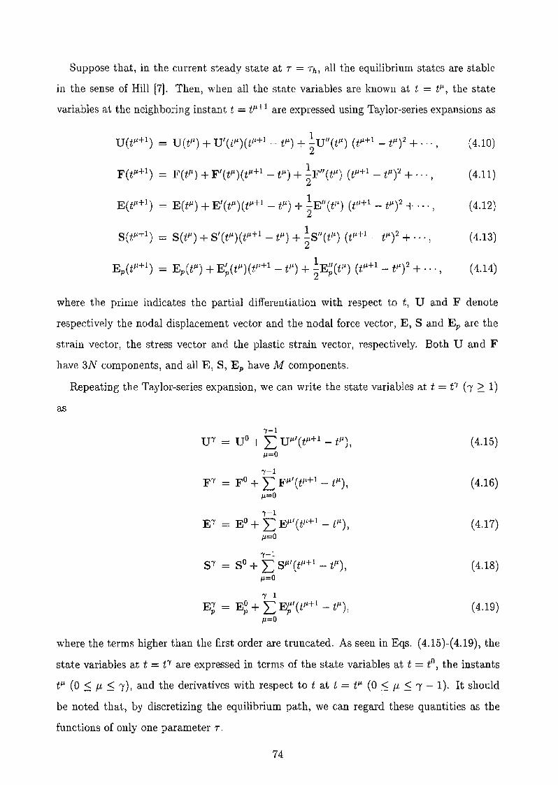
Suppose that, in the current steady state at T = Th, all the equilibrium states are stable
in the sense of Hill [7]. Then, when all the state variables are known at t = tli , the state
variables at the neighboring instant t = t li+! are expressed using Taylor-series expansions as
U(tJ.t+1) = V(tli ) + U'(tli) (til+l - t Ji ) + ~UI/(t/-l) (t JL+1 _ t Ji )2 +"',
F(til+!) = F(til ) + F'(til) (t Ji+1 - t JL ) + ~F//(tJi) (tJL+1 - til? + ... ,
E(til+!) = E(tli ) + E'(til) (t li+1 - til) + ~E/f(til) (tJi+! _ tli )2 + "',
1S(til+1
) = S(tJi ) + S'(tli)(tli+1 - til) + -SI/(t/-l) (t/-l+1 _ t li )2 + "',2
Ep(tli+1) = Ep(t Ji ) + E~(til)(tJL+l - t/-l) + ~E~(til) (til+l - t fl )2 + ... ,
(4.10)
(4.11)
(4.12)
(4.13)
(4.14)
where the prime indicates the partial differentiation with respect to t, V and F denote
respectively the nodal displacement vector and the nodal force vector, E, S and Ep are the
strain vector, the stress vector and the plastic strain vector, respectively. Both U and F
have 3N components, and all E, S, E p have M components.
Repeating the Taylor-series expansion, we can write the state variables at t = fY b 2 1)
as
")'-1
V")' = V O+ 2:= Vil'(til+l - til),fl=O
")'-1
F")' = F O + 2:= FJi'(tJi+1- tli),
1i=0
")'-1
E"l' = EO + 2:= EJi'(tJi+1- til),
tl=O
")'-1
S")' = SO + 2:= SJ.l'(tJi+1- til),
1-1=0
')'-1
E")' = EO + '"' E/-I'(til+1- tl-l)p p L.tP ,
il=O
(4.15)
(4.16)
(4.17)
(4.18)
(4.19)
where the terms higher than the first order are truncated. As seen in Eqs. (4.15)-(4.19), the
state variables at t = t"Y are expressed in terms of the state variables at t = to, the instants
til (0 :::; p, :::; 1'), and the derivatives with respect to t at t = tli (0 .-:; p, :::; l' - 1). It should
be noted that, by discretizing the equilibrium path, we can regard these quantities as the
functions of only one parameter T.
74
4.3.2 Tangent Stiffness Equations
In this subsection, the equations are shown for obtaining the partial derivatives with re
spect to t. For simplicity, we derive only the first-order derivatives. But more higher-order
derivatives can be obtained with the equations derived by differentiating the tangent stiffness
equations [17]. Suppose that all the state variables are known at t = tJ.I. Differentiating the
strain-displacement relations (4.1)-(4.3) with respect to t, we have the following equations
for t = t P
pI _ 8 c:J.I J.I'c: - -8puj •
u·z(4.20)
Summation convention is used for the subscripts i, j and k which are varied from 1 to 6
throughout this chapter. Differentiation of the equilibrium condition (4.4) yields
(4.21 )
Differentiating Eqs. (4.5)-(4.7), we have
in which TCP. is determined by
(4.22)
TCIL E
TCIL Etl C:' 2: 0
TCIL E, E' < 0
TCIL Et, C:' < 0
TCIL E, C:' > 0
in the elastic range,
for the loading response in tension,
for the unloading response in tension,
for the loading response in compression,
for the unloading response in compression.
(4.23)
(4.24)
(4.25)
(4.26)
(4.27)
Substituting Eqs. (4.20) and (4.22) into Eq. (4.21), we have
j J.!'1 = TkJ.!'.u~'Z 2) )
where
Assembling Eq. (4.28), we have the tangent stiffness equation for the total system
75
(4.28)
(4.29)
(4.30)
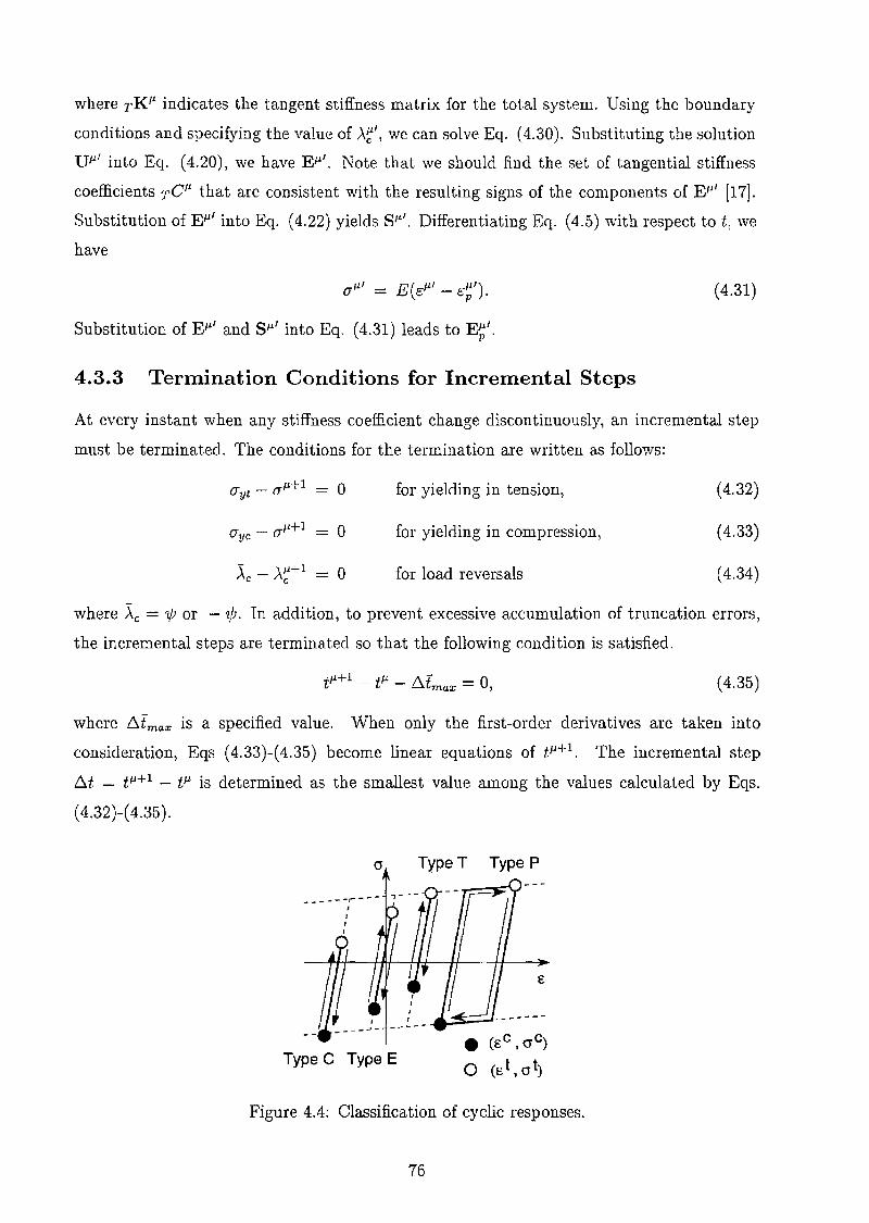
where TKIi indicates the tangent stiffness matrix for the total system. Using the boundary
conditions and specifying the value of At', we can solve Eq. (4.30). Substituting the solution
Dll' into Eq. (4.20), we have Ei-L'. Note that we should find the set of tangential stiffness
coefficients TCIi that are consistent with the resulting signs of the components of Ei-L ' [17].
Substitution of EJ-l' into Eq. (4.22) yields SIi'. Differentiating Eq. (4.5) with respect to t, we
have
(JJ1/ = E(cli' - c~').
Substitution of Eli' and SJi' into Eq. (4.31) leads to E~'.
4.3.3 Termination Conditions for Incremental Steps
(4.31)
At every instant when any stiffness coefficient change discontinuously, an incremental step
must be terminated. The conditions for the termination are written as follows:
(Jyt - a Ji+1 0
(lye - (JJi+l - 0
.:\. _ All+1 0e e
for yielding in tension,
for yielding in compression,
for load reversals
(4.32)
(4.33)
(4.34)
where Ae = 'ljJ or - 'ljJ. In addition, to prevent excessive accumulation of truncation errors,
the incremental steps are terminated so that the following condition is satisfied.
(4.35)
where .6.tmax is a specified value. When only the first-order derivatives are taken into
consideration, Eqs (4.33)-(4.35) become linear equations of t Jl+1• The incremental step
.6.t = i Jl+1 - til is determined as the smallest value among the values calculated by Eqs.
(4.32)-(4.35).
cr Type T Type P
Type C Type E• (t C , cr c)
o (Et , crt)
Figure 4.4: Classification of cyclic responses.
76
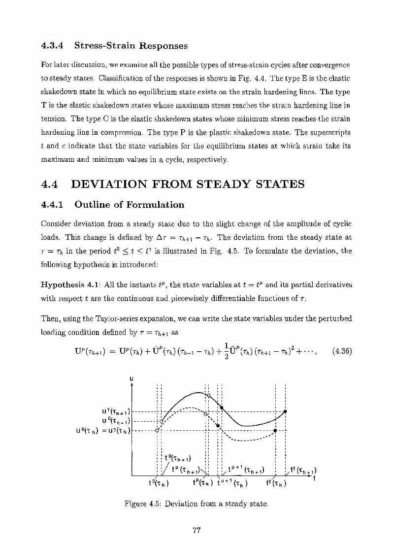
4.3.4 Stress-Strain Responses
For later discussion, we examine all the possible types of stress-strain cycles after convergence
to steady states. Classification of the responses is shown in Fig. 4.4. The type E is the elastic
shakedown state in which no equilibrium state exists on the strain hardening lines. The type
T is the elastic shakedown states whose maximum stress reaches the strain hardening line in
tension. The type C is the elastic shakedown states whose minimum stress reaches the strain
hardening line in compression. The type P is the plastic shakedown state. The superscripts
t and c indicate that the state variables for the equilibrium states at which strain take its
maximum and minimum values in a cycle, respectively.
4.4 DEVIATION FROM STEADY STATES
4.4.1 Outline of Formulation
Consider deviation from a steady state due to the slight change of the amplitude of cyclic
loads. This change is defined by 6T = Th+l - Th. The deviation from the steady state at
T = Th in the period to ::; t ::; rr is illustrated in Fig. 4.5. To formulate the deviation, the
following hypothesis is introduced:
Hypothesis 4.1: All the instants t l \ the state variables at t = t fJ and its partial derivatives
with respect t are the continuous and piecewisely differentiable functions of T.
Then, using the Taylor-series expansion, we can write the state variables under the perturbed
loading condition defined by T = Th+! as
(4.36)
uI I II I I, I II I I lI I l I ,I I I L ,
uY('th ,) ~~ ~~::::~~_~~__ :_L ~_
+ I I,;#' 0.1 I' Ia I' , I h. 'I I
U ('t h +,) -------: /' : :"it: : ,UO('t h) =UY('th) -------<17-------------~~--L·~~--------------,-it--,~
I I I I I...... ..",,'" I III II I ..... ...... Ii
I t I I I I II t I I I I II I 'I I I II I I I I I I
::to('th+1) :: : ::I I I I I I I
:: tJl('t h+,):: : t Jl + 1 ('t h+,) : :t
Figure 4.5: Deviation from a steady state.
77

'i. • fJ. 1 .. fJ. 2F (rhH) = FfJ.(Th) + F (T,,) (ThH - r,,) + 2"F (T,,) (T"H - Th) +"',
. fJ. 1 "}i. 2EJl.(T"H) = EIt(Th) + E (T,,) (ThH - T,,) + 2"E (n) (Th+l - Th) + ... I
. It 1 .. fJ. 2SfJ.(Th+l) = SfJ.(Th)+S (Th)(Th+l-Th)+-S (Th)(T"+l-Th) +"',
2
·It 1··,. 2E~(r"+l) = E~(Th) + Ep(Th) (ThH - rh) + -Ep(Th) (rh+l - Th) + ... ,
2
(4.37)
(4.38)
(4.39)
(4.40)
where dot indicates the differentiation with respect to T. For simplicity, our discussion in
this paper is restricted to the case where all the terms higher than first order are neglected.
Now our object is to obtain the derivatives with respect to T. A difficulty arises here
because no direct stress rate-strain rate relation such as Eqs. (4.23)-(4.26) is given. The
strategies to overcome this difficulty are outlined as follows:
1. To use the stress rate-strain rate relations obtained by differentiating (4.5), which is
valid in any equilibrium state, with respect to T. This idea was proposed by Uetani and
Kobayashi [16]. Since plastic strains are included in the stress rate-strain rate relations,
as shown in the next subsection, all the derivatives can be expressed as
(4.41)
(4.42)
(4.43)
(4.44)
where HfJ. and hfJ. are the constant matrix vector, respectively.
2. To express the plastic strain rates at t = tfJ. as
(4.45)
where GfJ. and gfJ. are the constant matrix and vector, respectively. This relation is
derived in the later subsection 4.4.3.
3. To obtain the recurrence equation that relates the plastic strain rates at the two con
secutive periodic instants t = to and t = f}' by substituting /L = 'Y into Eq. (4.45).
(4.46)
The plastic strain rate :It~ is obtained as the limit of the solution of the recurrence
equation (4.46) as I ~ 00. SUbstituting:lt~ into Eq. (4.45), we have :It;. Substitution
of :It; into Eqs. (4.41)-(4.44) yields the first-order derivatives at t = tfJ..
78

4.4.2 Rate Relations at Arbitrary Instants
In this subsection, it is shown that all the first~order derivatives with respect to Tare
expressed as Eqs. (4.41)-(4.44), which are the linear equations of :It;. Differentiating (4.1)
(4.4) I we have the rate forms of strain-displacement relations as
'Il _ a E1J
. IlE - 7lIiUi'
U Uj
The rate forms of equilibrium conditions are written as
it = ALa (all ~ e: + (Til aa: ~ Il Uj) .u Ui U i Uj
Differentiating Eq. (4.5) yields
'~l _ E('1l _ 'Il)(T - E cp '
(4.47)
(4.48)
(4.49)
Note that this relation is valid even if plastic loading occurs at t = til and that ill is
deliberately remained as unknowns in this formulation though E~' is usually eliminated in
the formulation for tracing equilibrium paths. Substitution of Eqs. (4.47) and (4.49) into
Eq. (4.48) leads to
(4.50)
where Ek& is the coefficient of uj and Ebf is the coefficient of i~. Assembling the rate
equations (4.50) yields the rate relations for the total system
(4.51)
. .where EK and EB are the coefficient matrices of U and Ep , respectively. By using the
boundary conditions and by arranging Eq. (4.51) as shown in Appendix A, we can express
F and U as
F' Il _ HJJ.E·J1. hll- I P + I'
U·JJ. - HJJ.E·JJ. hJ1.- u P + u'
(4.52)
(4.53)
in which HJ1. and hJJ. denote the constant matrix and constant vector, respectively, and the
subscripts f and u indicate the variables corresponding to F and U. Using the rate forms
of the compatibility condition (4.47) and the stress-strain relation (4.49), we have
E· JJ. - HJJ.E·Il + hll- e p e'
S· Il - HIlE'Il hJ1.- s p+ s'
where the subscripts e and s indicate that the variables refer to those for E and S.
79
(4.54)
(4.55)
4.4.3 Recurrence Relations between Consecutive Periodic Instants
• 0 • 'YLet us shown that the relation between Ep and Ep are expressed as the recurrence relation
(4.46). This is shown in two stages based on the procedure of the mathematical induction.
First, obviously, we have
(4.56)
o . Jlwhere G = I and gO = O. Next, assume that E p is assumed to be expressed as
(4.57)
and that til is written as
(4.58)
in which gf and gi are the constant vector and the constant, respectively, and the superscript
T indicates the transpose of the vector. Then our problem is to show that t;+l is written
as
(4.59)
The incremental relation between E~ and E~+l is expressed as
(4.60)
where the higher-order terms with respect to t more than first order are neglected. Differ
entiating Eq. (4.60) with respect to 7, we have
(4.61)
Here, from the assumptions, t; and til in Eq. (4.61) are expressed as the linear equations
of t~. The variables til, t ll+1 and E~' can be regarded as constants since they are the known. !
quantities in the current steady state at 7 = 7h. Since, as shown in Appendix B, both E~
and til+! are expressed as
(4.62)
(4.63)
where R~ and r~ are the constant matrix and the constant vector, respectively. Now we can. p+! . 0
express Ep as the linear equation of Ep .
80
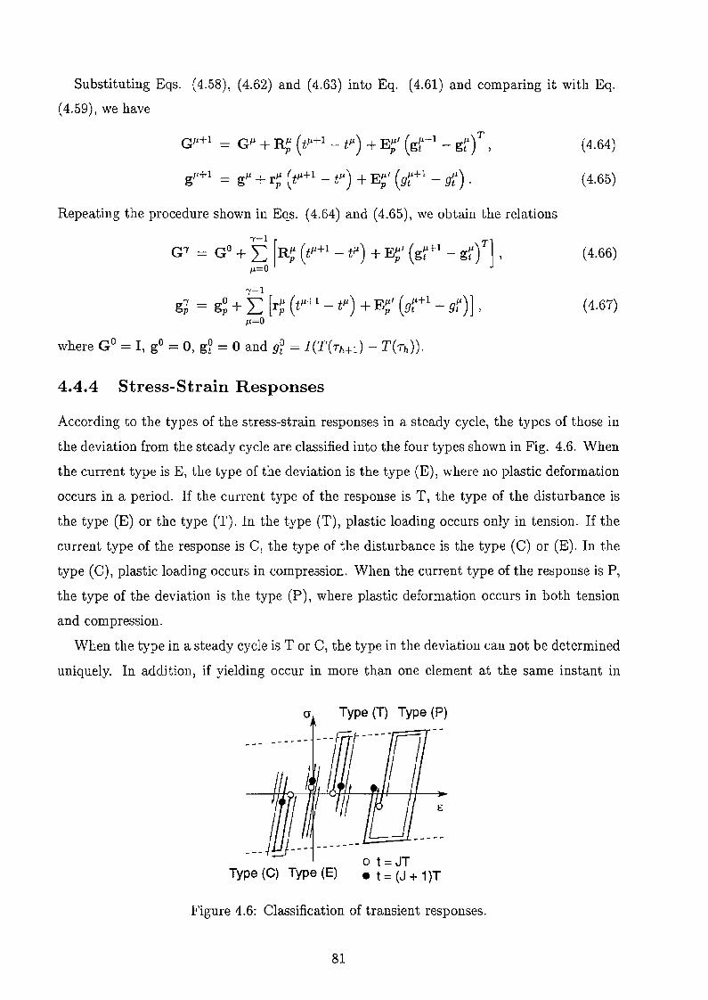
Substituting Eqs. (4.58), (4.62) and (4.63) into Eq. (4.61) and comparing it with Eq.
(4.59), we have
Gll+l = Gil + R~ (t ll+1 - til) + E~' (gt+1 - gr)T ,
gll+1 = gJ.l + r~ (tJ.l+1 - tJ.l) + E~' (gt+ 1- gr) .
Repeating the procedure shown in Eqs. (4.64) and (4.65), we obtain the relations
[-I
g; = g~ + L [r~ (t1H1- tJ.l) + E~' (gr+l - gn] ,
11=0
4.4.4 Stress-Strain Responses
(4.64)
(4.65)
(4.66)
(4.67)
According to the types of the stress-strain responses in a steady cycle, the types of those in
the deviation from the steady cycle are classified into the four types shown in Fig. 4.6. When
the current type is E, the type of the deviation is the type (E), where no plastic deformation
occurs in a period. If the current type of the response is T, the type of the disturbance is
the type (E) or the type (T). In the type (T), plastic loading occurs only in tension. If the
current type of the response is C j the type of the disturbance is the type (C) or (E). In the
type (C), plastic loading occurs in compression. When the current type of the response is P,
the type of the deviation is the type (P), where plastic deformation occurs in both tension
and compression.
When the type in a steady cycle is T or C, the type in the deviation can not be determined
uniquely. In addition, if yielding occur in more than one element at the same instant in
cr Type (T) Type (P)
Type (C) Type (E)
€
Figure 4.6: Classification of transient responses.
81

the steady-state response, the order of the instants in the deviation cannot be determined
uniquely. Hence if such situation takes place, the types of the response and the order of the
instants should be assumed in constructing the recurrence equation (4.46).
4.5 STABILITY OF STEADY STATES
4.5.1 Definition of Stability
Following the definition of stability of solution due to Liapunov [2], the concept of stability
of steady states is simply stated as "a steady state is stable if a small change in loading
condition leads to a small deviation in the responses". Note that the small change in the
loading condition is given as the level of external loads here, while that is given as initial
conditions in the definition by Liapunov.
The rigorous definition of the stability is stated as
Definition 4.1 For an arbitrary positive number E, if there exists a positive number (j such
that every solution with I~TI < 6satisfies the inequality ~U(t) < E for all times t ~ 0, the
steady state is called stable.
Here, ~U(t) is the norm defined by
~U(t) = IIU(T + 6.7, t) - V(T, t)111
~ {~[Un(T + L'l.T, t) - Un(T, tl]'rwhere the subscript n indicates the number of the component of U.
4.5.2 Stability Criterion
(4.68)
As shown in the previous section, if the type of the stress-strain responses under the per
turbed loading condition is assumed, the relation between the plastic strain rates at periodic
instants t = IT and t = (I + l)T are uniquely expressed in the form of recurrence equation
Eq. (4.46)
This equation can be partitioned as
{-:~-} = [-~~ ~ -] {-:n + {-:-}
82
(4.69)
where E indicate the plastic strain rates of the elements in which no plastic deformation
occurs in a period, E indicate those of the other elements, and G is the coefficient matrix
of E:. The displacement rate II is expressed as the linear equation of E~ as far as EK is
positive definite as shown in subsection 4.4.2. The stability criterion is therefore written in
terms of the eigenvalues of G as
Theorem 4.1 Suppose that the maximum absolute eigenvalue of G is less than one for all
the possible combinations of the types of the stress-strain response to the incremental change
in loading condition. And suppose that all the equilibrium states are stable in the sense of
Hill [7]. Then the steady state is stable.
Since the number of the combination are finite, it is theoretically possible to examine all the
possible combinations. It must be recognized here that, without this criterion, one has to
perform equilibrium path analysis for infinite number of the pattern change in the loading
conditions in order to ensure the stability. And it is generally very difficult to examine by
using the equilibrium analysis whether or not the transient response converges to a steady
state as I ~ 00 because of the accumulation of numerical errors.
However, if the number of elements exhibiting the type T or C becomes large, it seems
to virtually impossible to examine all the possible combinations. To obtain more practical
stability criterion that can be used in this case, the following two hypotheses are introduced.
Let GL indicate G that is constructed in the case where all the elements exhibiting the type
T and C exhibit (T) and (C), respectively. Then the hypotheses are given as:
Hypothesis 4.2 The values of the components of G are independent of the order of the
yielding times of the elements exhibiting type (T) or (C).
Hypothesis 4.3 The maximum absolute eigenvalue of GL is less than or equal to those of
G constructed for all the possible combinations of the types of the stress-strain response in
the perturbed response.
On the basis of Hypotheses 4.2 and 4.3, a more relaxed and practical stability criterion is
give by the following theorem.
Theorem 4.2 The steady state is stable if the maximum absolute eigenvalue of GL is less
than one.
Here, theorems 4.1 and 4.2 states the sufficient conditions for the stability of a steady state.
83
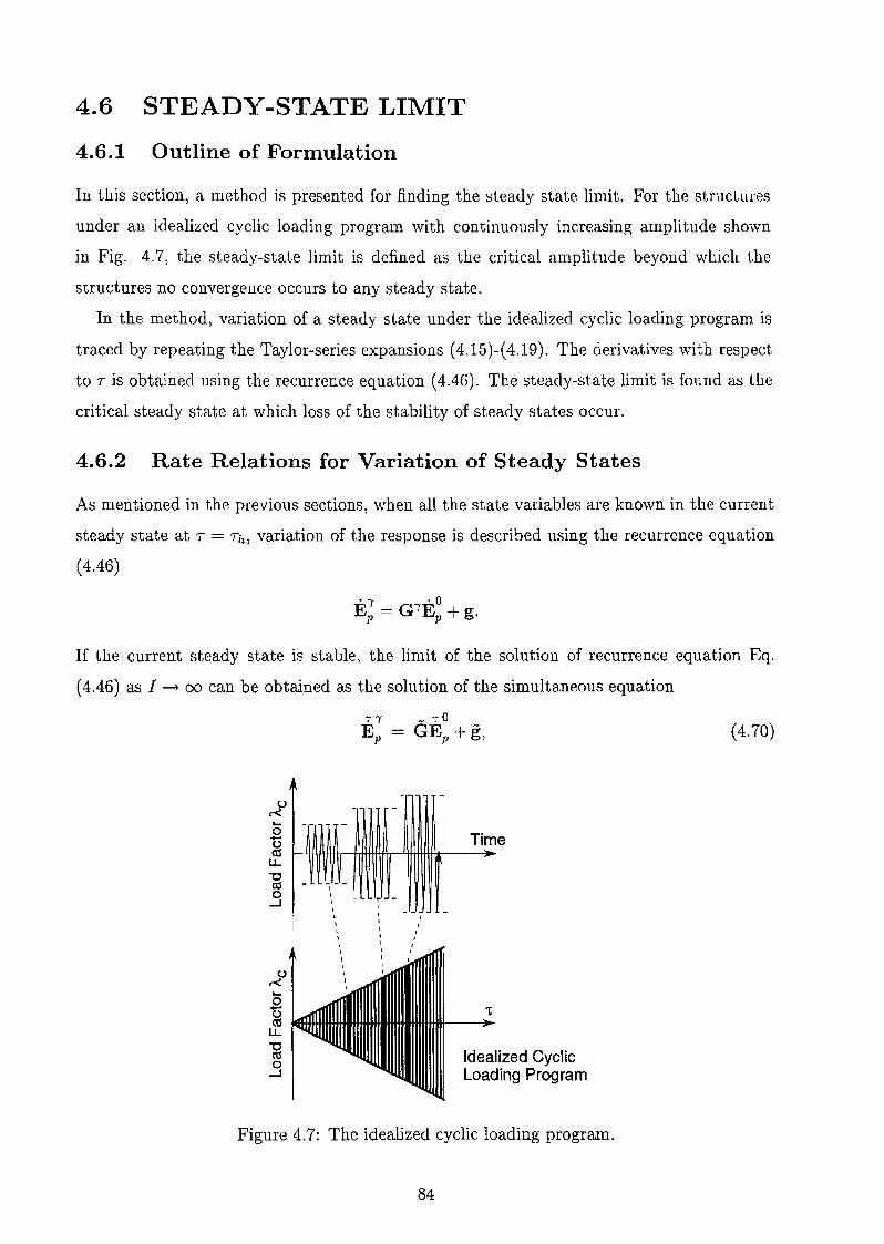
4.6 STEADY-STATE LIMIT
4.6.1 Outline of Formulation
In this section, a method is presented for finding the steady state limit. For the structures
under an idealized cyclic loading program with continuously increasing amplitude shown
in Fig. 4.7, the steady-state limit is defined as the critical amplitude beyond which the
structures no convergence occurs to any steady state.
In the method, variation of a steady state under the idealized cyclic loading program is
traced by repeating the Taylor-series expansions (4.15)-(4.19). The derivatives with respect
to 7 is obtained using the recurrence equation (4.46). The steady-state limit is found as tbe
critical steady state at which loss of the stability of steady states occur.
4.6.2 Rate Relations for Variation of Steady States
As mentioned in the previous sections, when all the state variables are known in the current
steady state at 7 = 7f" variation of the response is described using the recurrence equation
(4.46)
. l' . 0E p = G1'Ep + g.
If the current steady state is stable, the limit of the solution of recurrence equation Eq.
(4.46) as I ~ 00 can be obtained as tbe solution of the simultaneous equation
(4.70)
't
Idealized CyclicLoading Program
0,-<....0
Time.....r0
ct:.lIIU. I'
"'0ct:.l0
.....J
,-<0.....9gu.-go
....J
Figure 4.7: The idealized cyclic loading program.
84

-1' - 0Ep = Ep ,
... 0Ep = O.
(4.71)
(4.72)
Substituting the solution of the simultaneous equations into Eqs. (4.41)-(4.44) and (4.45),
we have all the derivatives at t = t Jl with respect to 'T.
4.6.3 Consistent Set of Stress-Strain Responses
When an element exhibits type T in the current steady state at 'T = 'Th, the type in the
deviation from the steady state is the type (T) or (E). Similar is the case \vhen an element
exhibits type C. In constructing the rate relations for variation of a steady state, we assume
the type in the deviation for the elements exhibiting the type C and T. On the other hand,
direction of the plastic deformation occurred in the transient process between two consecutive
steady states must be consistent with the assumed type of the transient response. Therefore,
for all the elements exhibiting the type T or the type C behavior, we should choose a set of
the stress-strain responses that are consistent with the signs of the resulting strain rates. In
addition, when yielding occur in more than one element at the same instant in the current
steady state, the order of the instants in the deviation may be different and cannot be
determined uniquely. The order is assumed in obtaining the rate relations, and the resulting
order should be checked whether they are consistent with the assumptions or not.
To find the consistent set of the stress-strain responses, we employ a trial and error
approach. In the trial and error approach, first, we assume the type of the stress-strain
responses and the order of instants if necessary. Then, the rate equations are constructed
and solved. The consistency is checked between the assumption and the results. This
procedure is continued until all the assumptions are consistent with the results.
4.6.4 Termination Conditions for Incremental Steps
When the types of the stress-strain responses in steady states change as shown in Fig. 4.8,
different types of the stress-strain responses in deviation should be used in constructing the
recurrence equation (4.46). Incremental steps 6.'T is therefore determined considering the
conditions for the transition of the types of the stress-strain responses in steady states.
The step length 6.'T is selected as the smallest positive value among the values calculated
from the following conditions (4.73)-(4.79):
85
0, (4.73)
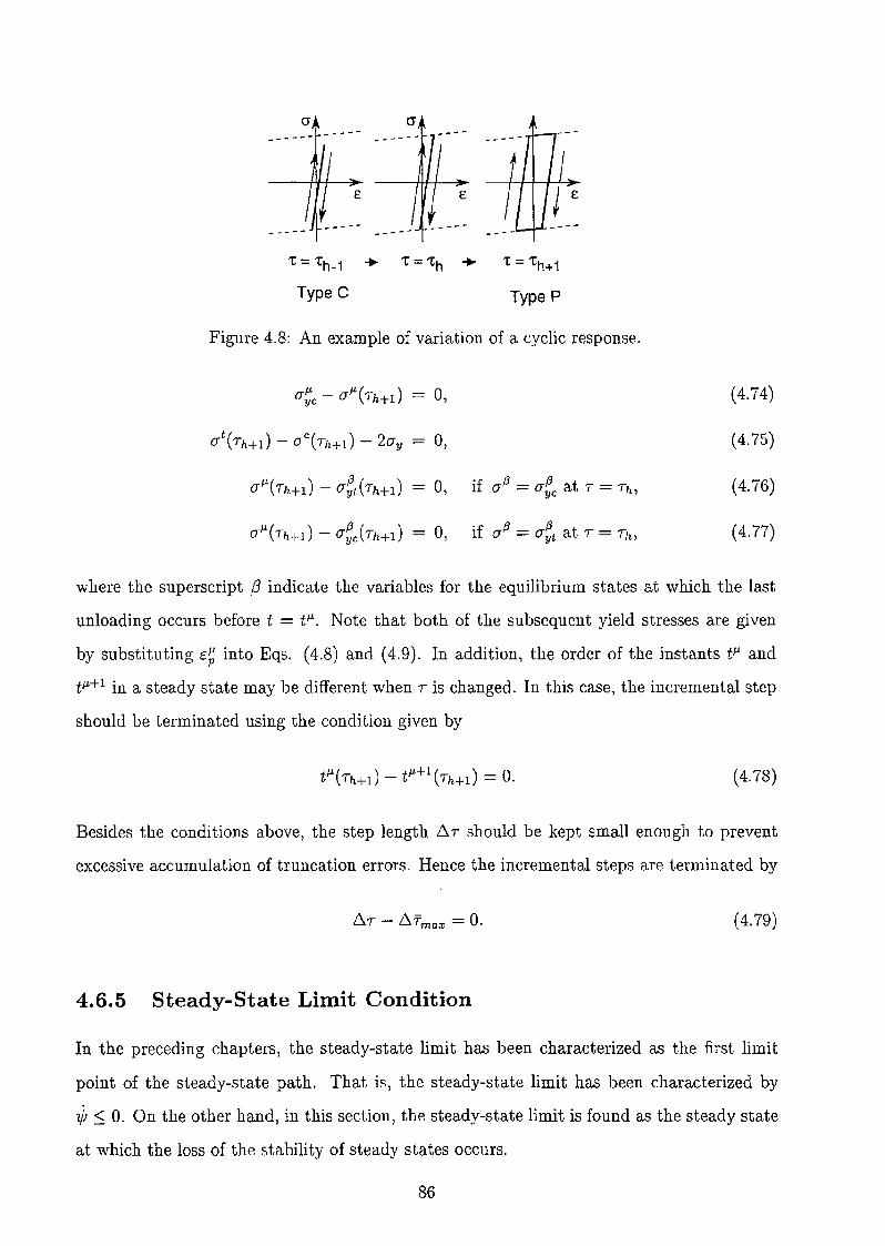
cr---~-
Type C Type P
Figure 4.8: An example of variation of a cyclic response.
Ii /L( ) - 0(Iyc - (J Th+l - , (4.74)
(4.75)
(4.76)
(4.77)
where the superscript f3 indicate the variables for the equilibrium states at which the last
unloading occurs before t = t li . Note that both of the subsequent yield stresses are given
by substituting E:~ into Eqs. (4.8) and (4.9). In addition, the order of the instants tli and
t li+1 in a steady state may be different when T is changed. In this case, the incremental step
should be terminated using the condition given by
(4.78)
Besides the conditions above, the step length l:!.T should be kept small enough to prevent
excessive accumulation of truncation errors. Hence the incremental steps are terminated by
D.T - D.Tmax = O.
4.6.5 Steady-State Limit Condition
(4.79)
In the preceding chapters, the steady-state limit has been characterized as the first limit
point of the steady-state path. That is, the steady-state limit has been characterized by
;p :::; O. On the other hand, in this section, the steady-state limit is found as the steady state
at which the loss of the stability of steady states occurs.
86
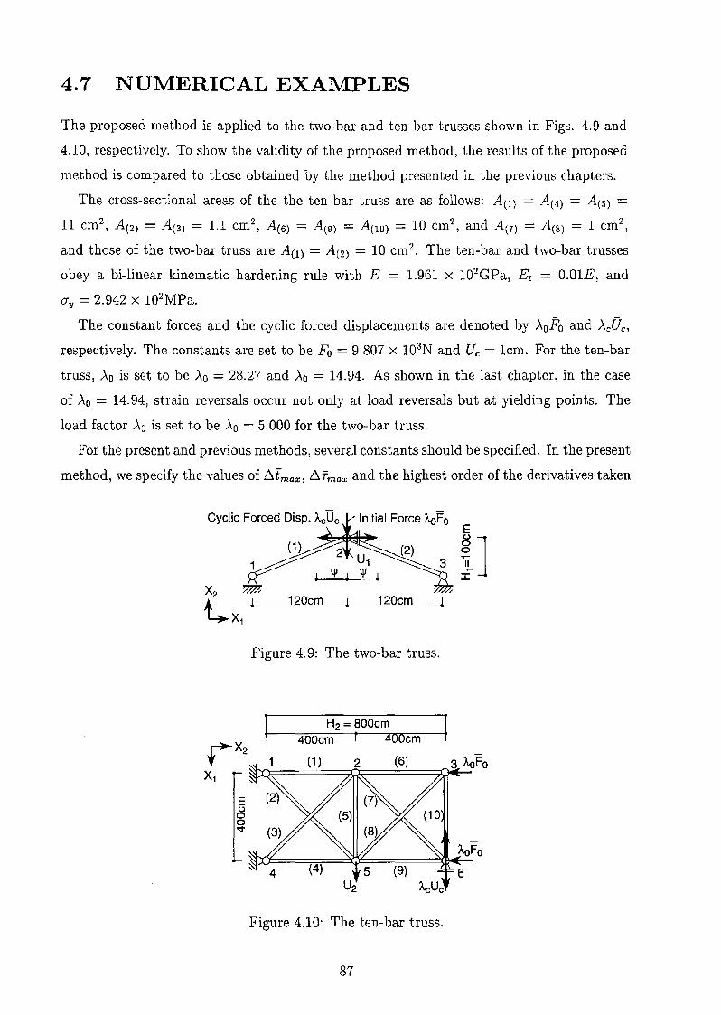
4.7 NUMERICAL EXAMPLES
The proposed method is applied to the two-bar and ten-bar trusses shown in Figs. 4.9 and
4.10, respectively. To show the validity of the proposed method, the results of the proposed
method is compared to those obtained by the method presented in the previous chapters.
The cross-sectional areas of the the ten-bar truss are as follows: A(1) = A(4) = A(5) =11 cm2
, A(2) = A(3) = 1.1 cm2, A(6) = A(9) = A(lO) = 10 cm2
, and A(7) = A(8) = 1 cm2,
and those of the two-bar truss are A(l) = A(2) = 10 cm2. The ten-bar and two-bar trusses
obey a bi-linear kinematic hardening rule with E = 1.961 x 10²GPa, E t = O.OlE, and
cry = 2.942 x 10²MPa.
The constant forces and the cyclic forced displacements are denoted by AoFo and A/)c,
respectively. The constants are set to be Fo = 9.807 x 10³N and Uc = 1cm. For the ten-bar
truss, >'0 is set to be >'0 = 28.27 and AO = 14.94. As shown in the last chapter, in the case
of >'0 = 14.94, strain reversals occur not only at load reversals but at yielding points. The
load factor AO is set to be AO = 5.000 for the two-bar truss.
For the present and previous methods, several constants should be specified. In the present
method, we specify the values of /limax , /lTmax and the highest order of the derivatives taken
J \jI I
120em
Initial Force AoFo
120em
En
Euoo'<:t
Figure 4.9: The two-bar truss.
H2 = aOOem400em r 400cm
Figure 4.10: The ten-bar truss.
87
AoFo
6

into account with respect to both t and T. Throughout the analysis, the higher-order terms
more than and equal to second order is neglected for both of the derivatives. For the ten
bar truss, these constants are I:!:.fmax = I:!:.fmax = 0.2 under AD = 28.27, and I:!:.fmax = 0.2
and I:!:.Tmax = 0.002 under AD = 14.94. And they are I:!:.[max = I:!:.Tmax = 0.001 for the
two-bar truss. On the other hand, in the previous method, I:!:.fmax and the highest order of
the derivatives taken into consideration with respect to T is specified. These are set to be
identical to those for the present method.
Variation of the maximum absolute eigenvalues of GL is shown in Figs. 4.11- 4.13. The
steady-state path obtained by the previous and the present method are illustrated in Figs.
4.14-4.16. The solid lines show the steady-state path obtained by the previous method. The
white circles indicate the results obtained by the present method. For the ten-bar truss
under AD = 28.27 and AD = 14.94 and the two-bar truss, the values of the steady-state limit
7/Jssl predicted by the present method are 7/Jssl = 2.590, 'l/Jssl = 13.17 and 7/Jssl = 0.1200)
respectively. Those obtained by the previous method are 7/Jssl = 2.589, 7/Jssl = 13.16 and
'l/Jssl = 0.1199. From these figures and values, it may be stated that good agreement is
observed between the steady state limits predicted by the previous and the current methods.
1.2 1.02
1 1.01
1.000.8
CD CD:::J :::J 0.99ro ro> 0.6 >l:: l::CD CD
0.9801 0>iIi iIi
0.40.97
0.2 0.96
0 0.950 0.03 0.06 0.09 0.12 0.15 0.112 0.114 0.116 0.118 0.12 0.122
Amplitude 'I' Amplitude 'I'
Figure 4.11: Variation of maximum absolute eigenvalue of GL for the two-bar truss.
88
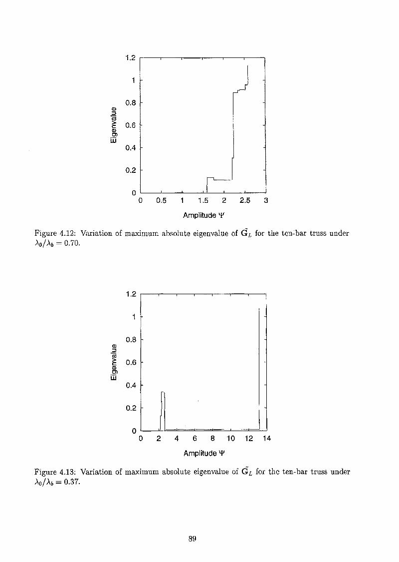
1.2
1 J0.8
Q)::Jas> 0.6c(I)0)
ill0.4
0.2
a ~a 0.5 1 1.5 2 2.5 3
Amplitude '¥
Figure 4.12: Variation of maximum absolute eigenvalue of GL for the ten":bar truss under>"0/>"b = 0.70.
1.2
1
0.8lD:::J«l> 0.6clD0)
ill0.4
0.2
0a 2 4 6 8 10 12 14
Amplitude '¥
Figure 4.13: Variation of maximum absolute eigenvalue of GL for the ten-bar truss under>"0/>"b = 0.37.
89
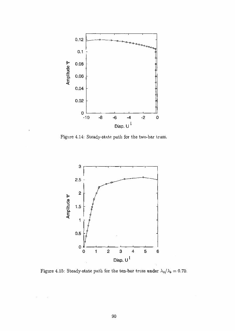
0.12
0.1
3-' 0.08Q)"0::::l~
0.06a.E«
0.04
0.02
0-10 -8 -6 -4 -2 0
Disp. U I
Figure 4.14: Steady-state path for the two-bar truss.
3
2.5
3-'2
Q)"0::::l 1.5;::a.E«
1
0.5
00 1 2 3 4 5 6
Disp. U I
Figure 4.15: Steady-state path for the ten-bar truss under Ao/Ab - 0.70.
90
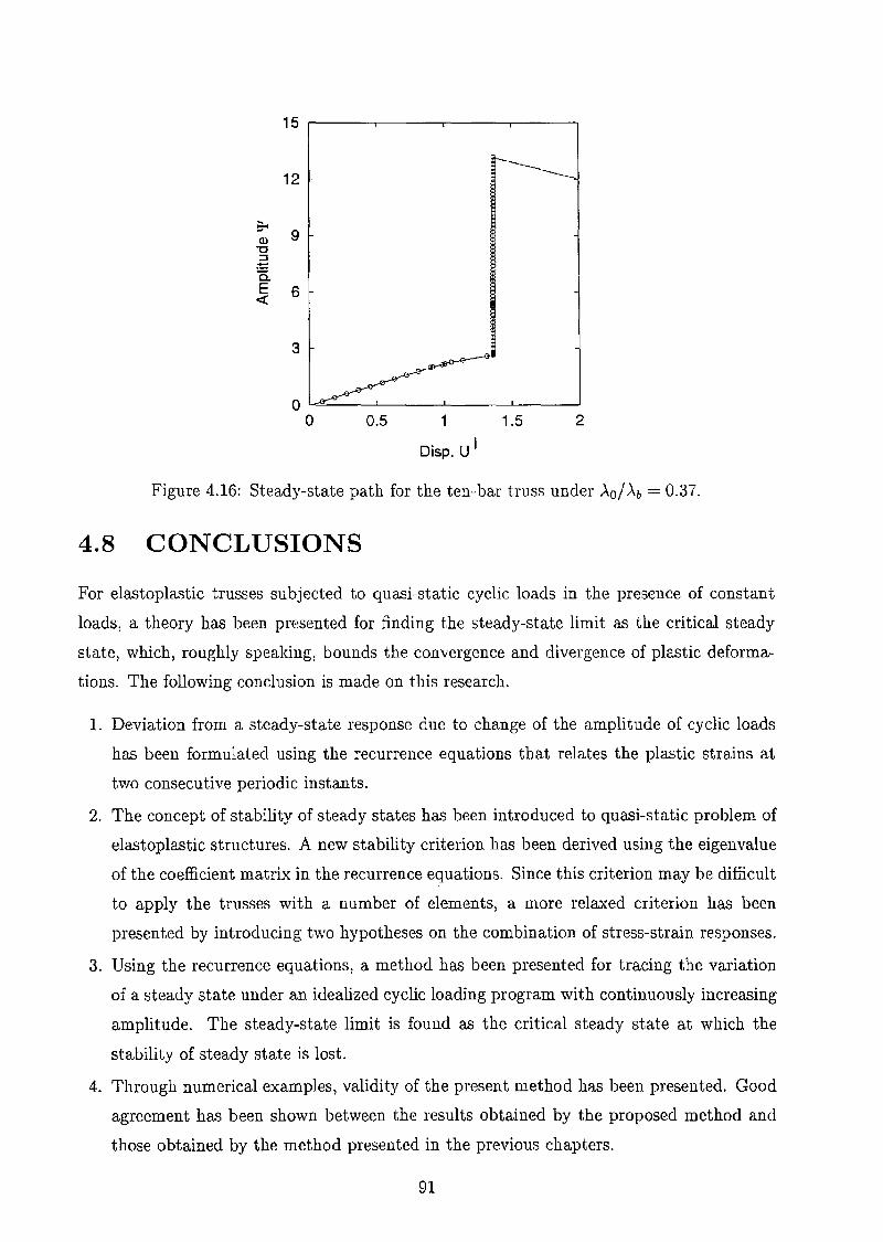
15 ,------r-------,------.-------,
21 1.5
Disp. U l0.5
o~----'--------'------'----'
o
12
~9Q)
-0:J
;t:::
C.E 6<t
3
Figure 4.16: Steady-state path for the ten-bar truss under AO/Ab = 0.37.
4.8 CONCLUSIONS
For elastoplastic trusses subjected to quasi-static cyclic loads in the presence of constant
loads, a theory has been presented for finding the steady-state limit as the critical steady
state, which, roughly speaking, bounds the convergence and divergence of plastic deforma
tions. The following conclusion is made on this research.
1. Deviation from a steady-state response due to change of the amplitude of cyclic loads
has been formulated using the recurrence equations that relates the plastic strains at
two consecutive periodic instants.
2. The concept of stability of steady states has been introduced to quasi-static problem of
elastoplastic structures. A new stability criterion has been derived using the eigenvalue
of the coefficient matrix in the recurrence equations. Since this criterion may be difficult
to apply the trusses with a number of elements, a more relaxed criterion has been
presented by introducing two hypotheses on the combination of stress-strain responses.
3. Using the recurrence equations, a method has been presented for tracing the variation
of a steady state under an idealized cyclic loading program with continuously increasing
amplitude. The steady-state limit is found as the critical steady state at which the
stability of steady state is lost.
4. Through numerical examples, validity of the present method has been presented. Good
agreement has been shown between the results obtained by the proposed method and
those obtained by the method presented in the previous chapters.
91
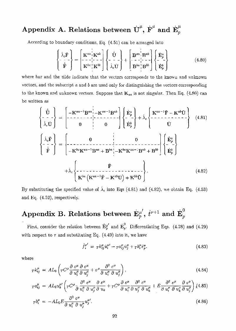
-/-t·f.l .. /),Appendix A. Relations between U , F and E p
According to boundary conditions , Eq. (4.51) can be arranged into
(4.80)
(4,82)
\vhere bar and the tilde indicate that the vectors corresponds to the known a.nd unknown
vectors, and the subscript a and b are used only for distinguishing the vectors corresponding
to the known and unknown vectors. Suppose that Rna is not singular. Then Eq, (4.80) can
be written as
[_~~~~I~~:-_~":O~I~:b_] {_:~_} +~, {_~":~I~~_~~?_} (4.81)
[-~~~~~:-~~:. -;~~L~~~":~~~,-;~~.-] {-:~-}
+~, {-~,~ (~:"~~f ~!~:'D); ~~O-}.By substituting the specified value of 'xc into Eqs (4.81) and (4,82)1 we obtain Eq, (4,53)
and Eq. (4.52), respectively.
, I . . 0Appendix B. Relations between E~ , t V+1 and Ep
First, consider the relation between E~' and E~. Differentiating Eqs. (4.28) and (4.29)
with respect to 7 and substituting Eq. (4.49) into it, we have
(4.83)
where
92

Assembling Eq. (4,83), we have the equation for the total system
(4.87)
. I . 1.1 • rwhere rK, rA and rB are the coefficient matrices of UIl, U and Ep . Substituting Eqs.
(4.53) and (4.57) into Eq. (4.87) and arranging it, we obtain
U· "I R"E'o 1.1,.. = ;:; p +ru '
Differentiating Eqs. (4.20), (4.22) and (4.31) with respect to r, we have
'Il' _ 82EJ1, J.lI , J.l a f: . /.II
E - ~ J1,..::l rUiUj+--u"U Uj U Uj a Ui l
irJ.l1 = rCJ.liJ.lI,
By using these relations, other state variables can be expressed as
E· J1,' - RJ.lE'0 /.Ip - p p + r p '
(4.88)
(4.89)
(4.90)
(4.91)
(4.92)
(4.93)
(4.94)
(4.95)
. . 0Next consider the relation between tV+! and E p . Differentiation of Eqs. (4.32)-(4.35)
yields
. . J.l+l = 0 for yielding in tension, (4.96)CTyt - a
. . JJ+! = 0 for yielding in compression j (4,97)CTye - CT
~ _ ~JJ+l = 0 for load reversals, (4.98)C e
ill+! - iJ.l - b.tmax = 0, .for truncation errors (4.99)
where
_. _ EEt 'J1,ayt - O"yc- E-EtEp,
irJJ+l = irll + ir JJI (t l.l+1- tJJ) + all' (tJ.l+1 - t JJ ) ,
93
(4.100)
(4.101)
(4.102)
(4.103)
(4.104)
From the assumption) tl-' is written as the linear equation of E~, and tl-'+! , tl-' and all the partial
derivatives with respect t are known variables. Hence, by arranging Eqs. (4.96)-(4.99), tv+!
is expressed as
t'l-'+1 IL+ITE'0 + 1-'+1= gt . p 9t '
94
(4.105)
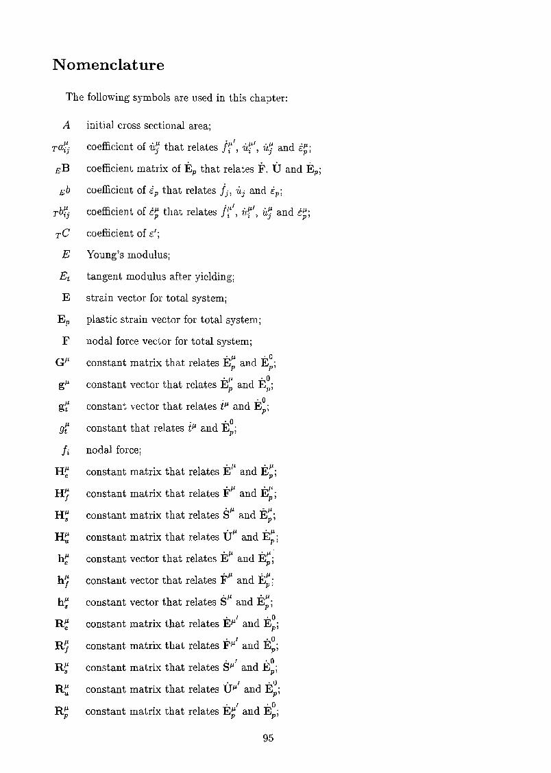
Nomenclature
The following symbols are used in this chapter:
A
T al!'·lJ
TC
E
E
F
GIL
g!J.
gf
gi
HiHIL
s
R~p
initial cross sectional area;
coefficient of u'; that relates ir', uri, 1L'; and i~j
coefficient matrix of Ep that relates F, U and Epj
coefficient of i p that relates i j , Uj and i p ;
coefficient of i~ that relates ir', uri, u'; and i~;
coefficient of c:';
Young's modulusj
tangent modulus after yielding;
strain vector for total system;
plastic strain vector for total system;
nodal force vector for total system;· IL . 0
constant matrix that relates E p and Ep ;
" jJ , 0constant vector that relates Ep and Epi
" . 0constant vector that relates tJ.t and Ep ;
• ' 0constant that relates tIL and Ep ;
nodal force;
'IL "ILconstant matrix that relates E and Ep ;
" IL • ILconstant matrix that relates F and E p ;
, IL • jJ
constant matrix that relates Sand E p ;
"IL 'ILconstant matrix that relates U and E p ;
. IL " IL .constant vector that relates E and E p ;
" IL • ILconstant vector that relates F and Ep i
'JL "I.tconstant vector that relates Sand Ep ;
" " 0constant matrix that relates EJ.t and Epi
., ' 0constant matrix that relates FJ.t and Epi
· , ,0constant matrix that relates SJ.l and Epi
• I ' 0constant matrix that relates UIL and Ep ;
· I ' 0constant matrix that relates E~ and Ep ;
95
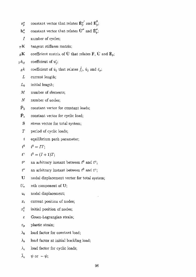
r 11p
I
L
Lo
M
N
S
T
t
fY
tfJ.
U
• I • °constant vector that relates E~ and E p ;
. fl . 11constant vector that relates U and E p ;
number of cycles;
tangent stiffness matrix;
coefficient matrix of U that relates F, U and t p ;
coefficient of uj;
coefficient of Uj that relates Ii, Uj and ip;
current length;
initial length;
number of elements;
number of nodes;
constant vector for constant loads;
constant vector for cyclic load;
stress vector for total system;
period of cyclic loads;
equilibrium path parameter;
to = IT;
to = (I + l)T;
an arbitrary instant between to and t";
an arbitrary instant between to and t";
nodal displacement vector for total system;
nth component of U;
nodal displacement;
current position of nodes;
initial position of nodes;
Green-Lagrangian strain;
plastic strain;
load factor for constant load;
load factor at initial buckling load;
load factor for cyclic loads;
7/J or - 7/J;
96
0-
o-yc
second Piola-Kirchhoff stress;
initial tensile yield stress;
o-y = (1 - EdE)o-y;
subsequent yield stress in compression;
subsequent yield stress in tension;
steady-state path parameter;
an arbitrary value of r;
of equilibrium path parameter;
U(r + ~Tl t) - U(r, t);
norm of ~U;
maximum allowable value of ~t;
increment of steady-state path parameter;
maximum allowable value of ~T;
amplitude of Ac ;
amplitude at steady-state limit;
Superscripts
t variables for the equilibrium states at strain reversals in tension;
c variables for the equilibrium states at strain reversals in compression;
o variables for the equilibrium states at t = to;
fL variables for the equilibrium states at t = til;
v variables for the equilibrium states at t = tV;
'Y variables for the equilibrium states at t = t-r;
Signs
() derivatives with respect to T;
()' derivatives with respect to t.
97
References
[1] A. M. Liapunov. The General Problem of the Stability of Motion. Taylor & Francis,
London, 1992. Translated and edited by A. T. Fuller.
[2] P. Z. Bazant and L. Cedolin. Stability of Structures. Oxford University Press, New
York, 1991.
[3] AIl. Collapse Analysis of Structures, volume 1. Maruzen, 1997. (in Japanese).
[4] W. T. Koiter. On the Stability of Elastic Equilibrium. Ph.D dissertation, 1945, Delft,
Holland, 1967. English Translation, NASA, TTF-10833.
[5] J. M. T. Thompson. A general theory for the equilibrium and stability of discrete
conservative systems. Zeitschrift fur Angewandte Mathematik und Physik, 20:794-846,
1969.
[6] J. M. T. Thompson and G. W. Hunt. A general theory of Elastic Stability. John Wiley
& Sons, New York, 1973.
[7] R. Hill. A general theory of uniqueness and stability in elastic-plastic solids. Journal of
the Mechanics and Physics of Solids, 6:236-249, 1958.
[8] J. M. T. Thompson and H. B. Stewart. Nonlinear Dynamics and Chaos. John Wiley &
Sons Ltd., 1986.
[9] J. Guckenheimer and P. Holmes. Nonlinear Oscillations, Dynamical Systems, and Bi
furcations of Vector Fields. Springer, New York, 1983.
[10] S. Wiggins. Introduction to Applied Nonlinear Dynamical Systems and Chaos. Springer,
New York, 1990.
[11] W. T. Koiter. General theorems for elastic-plastic structures. In J. N. Sneddon and
R. Hill, editors, Progress in Solid Mechanics, volume 1, pages 167-221, North Holland,
Amsterdam, 1960.
[12] J. A. Konig. Shakedown of Elastic-Plastic Structures. Elsevier, Amsterdam, 1987.
[13] K. Uetani and T. Nakamura. Symmetry limit theory for cantilever beam-columns sub
jected to cyclic reversed bending. Journal of the Mechanics and Physics of Solids,
31(6):449-484, 1983.
[14] K. Uetani. Symmetry Limit Theory and Steady-State Limit Theory for Elastic-Plastic
Beam-Columns Subjected to Repeated Alternating Bending. PhD thesis, Kyoto Univer
sity, 1984. (in Japanese).
98
[15] K. Uetani and T. Nakamura. Steady-state limit theory for cantilever beam-columns sub
jected to cyclic reversed bending. Journal of Structural and Construction Engineering,
AIJ, (438):105-115, 1992.
[16] K. Uetani and M. Kobayashi. Steady-state path analysis of continua subjected to alter
nating plastic deformation (analysis of elastic perfectly plastic solids). In Summaries,
1991 Meeting of the Architectural Institute of Japan, pages 267-268, 1991.
[17] Y. Yokoo, T. Nakamura, and K. Uetani. The incremental perturbation method for large
displacement analysis of elastic-plastic structures. International Journal for Numerical
Methods in Engineering, 10:503-525, 1976.
99


Chapter 5
Concluding Remarks
For elastoplastic trusses subjected to an idealized cyclic loading program with continuously
increasing amplitude, two methods have been presented for finding the steady-state limit,
which bounds the convergence and divergence of plastic deformations. The former method
has been presented in chapters 2 and 3, and the later has been presented in chapter 4.
Serious difficulty arises when the previous steady-state limit theory, originally developed
for cantilever beam-columns, is applied to trusses. The previous steady-state limit theory
was constructed based on the fundamental hypothesis that strain reversals in a steady state
occur only at load reversals. But this hypothesis may not be valid in trusses. This difficulty
is overcome in the former method by relaxing the hypothesis so that the strain reversals due
to yielding are taken into consideration. In the later method, this hypothesis is completely
excluded.
Moreover, in chapter 4, the concept of the stability of steady states has been introduced
to the quasi-static problem of elastoplastic trusses under cyclic loading. A new stability
criterion has been derived. And a more practical criterion has been given by introducing
the two hypotheses concerning the combination of the types of stress-strain responses. In
the former method presented in chapter 2 and 3, the steady-state limit is characterized as
the first limit point of the steady-state path, which represents the variation of steady state
under the idealized cyclic loading program. In contrast, the steady-state limit is found as the
steady state at which the stability of the steady states is lost in the later method presented
in chapter 4. Since the former method yields only steady states, which may be stable or
unstable, the characterization of the steady-state limit in the later method is more desirable.
Through numerical examples, validity of the two methods have been demonstrated. Good
agreements have been observed between the results obtained by the former method and those
obtained by the conventional response analysis if the loading conditions for these analyses
are close enough. Verification of the later method has been given by showing the good
101

agreement between the results obtained by the former and the later methods. It is worth
noting that, though this is not a quantitative result, the steady-state limits, defined under
an idealized cyclic loading program with continuously increasing amplitude, provide lower
bounds for the limiting values of convergence obtained by the response analysis performed
under the two typical and realistic cyclic loading programs.
There is a trade-off between the proposed two methods in tracing the steady-state path.
In the former method, no equilibrium path is needed to be traced. This is an advantage.
But, the size of simultaneous equations might be very large when the number of the elements
exhibiting plastic shakedown becomes large. This is a disadvantage. On the other hand, the
drawback of the later method is that one must perform equilibrium analysis, though only
for one cycle. The advantage of the later method is that the size of simultaneous equations
is generally much smaller than that in the former method. Hence, if the number of the
elements exhibiting plastic shakedown is not so large, the former method is more suitable
than the later method. Otherwise, the later method may be better. It should be noted that
these drawbacks are not inherent and may be overcome by making effort on the numerical
efficiency.
Throughout this thesis, only trusses are treated as the simplest finite dimensional struc
ture. But once the backbone procedure is developed for a simplified model, then it is expected
to provide a guideline for developing the procedures for practically acceptable models. The
methods and theories presented in this thesis can be easily extended to the arbitrarily shaped
structures whose behavior is described by uni-axial stress-strain relations. The later method
is expected to be directly applicable to three dimensional continua with almost no restric
tion. Furthermore, the later method appears to be suitable for taking into account dynamic
effects.
This conclusion ends with the topics of our future research:
1. To develop more efficient method based on the present methods.
2. To exclude the hypothesis on the combination of the types of stress-strain cyclic re
sponse. This is expected to lead to a uniqueness criterion of variation of a steady state.
3. To derive the stability criterion of a steady-state response taking dynamic effects into
account.
102