Embed Size (px)
Citation preview
The Spread of Industry:spatial agglomeration in economic development*
Diego PugaCentre for Economic Performance,
London School of Economics
Anthony J. VenablesLondon School of Economics
and Centre for Economic Policy Research
CENTRE for ECONOMIC PERFORMANCEDiscussion Paper No. 279, February 1996
ABSTRACT: This paper describes the spread of industry fromcountry to country as a region grows. All industrial sectors areinitially agglomerated in one country, tied together by input-output links between firms. Growth expands industry more thanother sectors, bidding up wages in the country in which industryis clustered. At some point firms start to move away, and whena critical mass is reached industry expands in another country,raising wages there. We establish the circumstances in whichindustry spills over, which sectors move out first, and which aremore important in triggering a critical mass.
* This paper was produced as part of the Programme on International Economic Performance at theUK Economic and Social Research Council funded Centre for Economic Performance, London Schoolof Economics. We thank participants in the NBER-TCER-CEPR Conference on Economic Agglomerationfor helpful discussion, Sigbjorn Sodal and a referee for useful comments, and Francisco Requena forproviding us with data on real earnings for East Asian economies. Financial support from the Bancode España (Puga) and the Taiwan Cultural Institute (Venables) is gratefully acknowledged.
KEY WORDS: location, agglomeration, industrialisation, linkages.JEL CLASSIFICATION: F12, O14, R12.
Addresses:
Diego Puga Anthony J. VenablesCentre for Economic Performance Department of EconomicsLondon School of Economics London School of EconomicsHoughton Street Houghton StreetLondon WC2A 2AE, UK London WC2A 2AE, UK
Email: [email protected] Email: [email protected]
1. Introduction
During the last three decades industry has spread from Japan to several of its East
Asian neighbours. In 1965 manufacturing absorbed nearly one of every four workers
in Japan, against one in six in Taiwan, one in eight in the Philippines, or one in eleven
in South Korea. Japanese manufacturing workers then earned over one and a half
times as much as their Philippine colleagues, and three times as much as
manufacturing workers in South Korea and Taiwan, measured on a purchasing power
parity (PPP) basis.
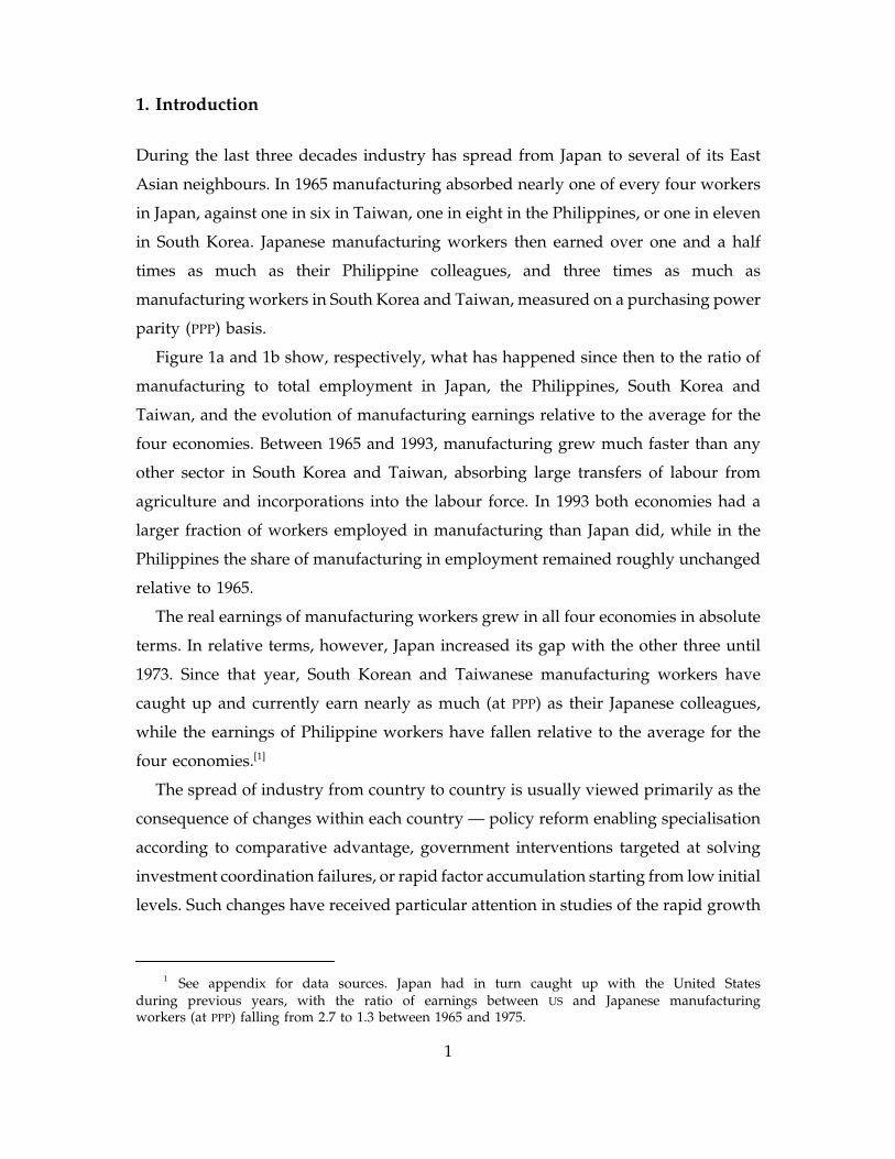
Figure 1a and 1b show, respectively, what has happened since then to the ratio of
manufacturing to total employment in Japan, the Philippines, South Korea and
Taiwan, and the evolution of manufacturing earnings relative to the average for the
four economies. Between 1965 and 1993, manufacturing grew much faster than any
other sector in South Korea and Taiwan, absorbing large transfers of labour from
agriculture and incorporations into the labour force. In 1993 both economies had a
larger fraction of workers employed in manufacturing than Japan did, while in the
Philippines the share of manufacturing in employment remained roughly unchanged
relative to 1965.
The real earnings of manufacturing workers grew in all four economies in absolute
terms. In relative terms, however, Japan increased its gap with the other three until
1973. Since that year, South Korean and Taiwanese manufacturing workers have
caught up and currently earn nearly as much (at PPP) as their Japanese colleagues,
while the earnings of Philippine workers have fallen relative to the average for the
four economies.[1]
The spread of industry from country to country is usually viewed primarily as the
consequence of changes within each country — policy reform enabling specialisation
according to comparative advantage, government interventions targeted at solving
investment coordination failures, or rapid factor accumulation starting from low initial
levels. Such changes have received particular attention in studies of the rapid growth
1 See appendix for data sources. Japan had in turn caught up with the United Statesduring previous years, with the ratio of earnings between US and Japanese manufacturingworkers (at PPP) falling from 2.7 to 1.3 between 1965 and 1975.
1

FIGURE 1aManufacturing employment relative to total employment
FIGURE 1bMonthly manufacturing earnings relative to the average for the four economies (at PPP)
1965 1970 1975 1980 1985 1990
0
0.5
1
1.5
2
year
rela
tive
wag
es
1965 1970 1975 1980 1985 1990
0.05
0.1
0.15
0.2
0.25
0.3
0.35
0.4
year
man
ufa
ctu
ring
sha
re in
em
ploy
men
t
Japan
Philippines
South Korea
Taiwan
Sources: see appendix
Philippines
Japan
South Korea
Taiwan
Sources: see appendix
2
of manufacturing production across the newly industrialising countries (NICs) of East
Asia (see, e.g, Little, 1994; Rodrik, 1995; and Young, 1995).
While not denying the importance of these considerations, in this paper we seek
to develop an alternative approach to the way in which industry spreads between
countries. We suppose that all countries are similar, or even identical, in underlying
structure, yet show that the distribution of industry may not be uniform across
countries and that industrialisation may spread in a series of waves from country to
country. The approach is based on a tension between agglomeration forces, which
tend to hold industry in a few locations, and wage differences (or more generally,
factor supply considerations) which encourage the dispersion of industry.
The basic idea runs as follows. Suppose that countries have identical technology
and endowments, and may contain two sectors, agriculture and industry. Firms in the
industrial sector are imperfectly competitive and are linked by an input-output
structure, which —as in Krugman and Venables (1995), and Venables (1996)— creates
forward and backward linkages. If there are some trade or transport costs, then
proximity to firms supplying intermediates reduces costs and gives rise to cost (or
forward) linkages. The presence of firms using intermediate goods raises sales and
profits of intermediate goods suppliers, and creates demand (or backward) linkages.
The interaction of these forces creates pecuniary externalities, encouraging the
agglomeration of industry so that, if these forces are strong enough, industry will be
concentrated in a single country (label it country 1). Wages in this country will be
higher than elsewhere, but the positive pecuniary externalities will compensate for the
higher wage costs.
Now suppose that some (exogenous) force increases the size of the industrial sector
relative to agriculture. This bids up wages in country 1 relative to wages elsewhere,
and there comes a point at which it becomes profitable for some industrial firms to
move out of country 1 to another country, say 2. As this process continues so firms
in 2 begin to benefit from the forward and backward linkages to other firms, and a
‘critical mass’ is reached. At this point there is rapid —although not necessarily
discontinuous— expansion of country 2 industry, accompanied by an increase in the
country 2 wage. The equilibrium now involves countries 1 and 2 industrialised and
with higher wages than elsewhere.
3
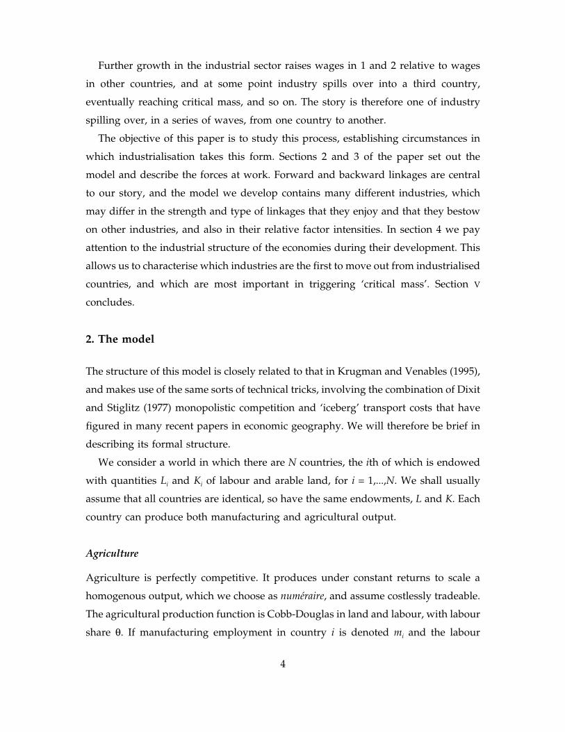
Further growth in the industrial sector raises wages in 1 and 2 relative to wages
in other countries, and at some point industry spills over into a third country,
eventually reaching critical mass, and so on. The story is therefore one of industry
spilling over, in a series of waves, from one country to another.
The objective of this paper is to study this process, establishing circumstances in
which industrialisation takes this form. Sections 2 and 3 of the paper set out the
model and describe the forces at work. Forward and backward linkages are central
to our story, and the model we develop contains many different industries, which
may differ in the strength and type of linkages that they enjoy and that they bestow
on other industries, and also in their relative factor intensities. In section 4 we pay
attention to the industrial structure of the economies during their development. This
allows us to characterise which industries are the first to move out from industrialised
countries, and which are most important in triggering ‘critical mass’. Section V
concludes.
2. The model
The structure of this model is closely related to that in Krugman and Venables (1995),
and makes use of the same sorts of technical tricks, involving the combination of Dixit
and Stiglitz (1977) monopolistic competition and ‘iceberg’ transport costs that have
figured in many recent papers in economic geography. We will therefore be brief in
describing its formal structure.
We consider a world in which there are N countries, the ith of which is endowed
with quantities Li and Ki of labour and arable land, for i = 1,...,N. We shall usually
assume that all countries are identical, so have the same endowments, L and K. Each
country can produce both manufacturing and agricultural output.
Agriculture
Agriculture is perfectly competitive. It produces under constant returns to scale a
homogenous output, which we choose as numéraire, and assume costlessly tradeable.
The agricultural production function is Cobb-Douglas in land and labour, with labour
share θ. If manufacturing employment in country i is denoted mi and the labour
4
market clears, agricultural output is (Li – mi)θ Ki
(1 – θ), and the wage in the economy
is
(1)wi
θ (Li
mi)(θ 1) K(1 θ)
i, i 1,...,N .
Manufacturing
Manufacturing is composed of S different sectors or industries, each of which is
assumed to be monopolistically competitive. The number of industry s firms operating
in country i is denoted nis and endogenously determined. Firms enter and exit in
response to positive and negative profits respectively, so at equilibrium profits are
exhausted. In each industry, a large number of differentiated goods can be produced
under increasing returns to scale. All potential varieties are symmetric, so at
equilibrium each firm produces a different one and charges a producer price pis.
Shipments of industrial goods are subject to ‘iceberg’ transportation costs —that is,
a fraction of any shipment melts away in transit. The number of units that must be
shipped from country i in order that one unit arrives at j is denoted τi,j , which we
assume to be same for all industries.
Each industry’s products can be aggregated via a CES function to yield a composite
that is used both as a consumption good and as an intermediate input. These CES
functions may be represented indirectly by CES price indices, qis. In each country each
industry’s price index is defined over products supplied from all sources, so takes the
form:
(2)q si
N
j 1
n sj(p s
jτ
j, i)(1 σ)
1 (1 σ)
,
where σ (> 1) is a measure of product differentiation.
The cost function of a single industry s firm in location i is:
(3)C si
(α β x si) 1ηs
w(1 ηs S
r 1µr, s )
i
S
r 1
(q ri)µr, s
.
5
We assume a fixed input requirement of α and a constant marginal input requirement
β. The input is a Cobb-Douglas aggregate of labour, agricultural and manufactured
products. The share of agriculture in the s industry is ηs, and agriculture has price 1.
The share of industry r in the s industry is µr, s , and qir is the price index of industry
r in country i, where all industry r varieties enter the composite intermediate and are
appropriately aggregated by the CES form of expression (2). Shares sum to unity, so
the labour coefficient is as given, and its price is the local wage, wi .
Preferences
The representative consumer in each nation has quasi-homothetic preferences over
agriculture (the numéraire) and the S CES aggregates of industrial goods. The indirect
utility of the representative consumer in country i is
(4)Vi
1 (1 S
s 1γ s )
S
s 1
(q si) γ s
(yi
e0 ) ,
where yi is income, and e0 is the subsistence level of agricultural consumption.
General equilibrium
Expenditure on each manufacturing industry in each country can be derived from (3)
and (4) as
(5)e si
γ s wim
i(L
im
i)θ K (1 θ)
ie0
S
r 1
µs,r n rip r
ix r
i.
The first term is the value of consumer expenditure, and the second the value of
intermediate demand. Consumers have a linear expenditure system (indirect utility
function given by (4)), so devote the first e0 of their income to agriculture, and
proportion γ s of their income above this level to expenditure on industry s products.
In the square brackets, the first term is wage income in manufacturing, and the
second is income generated in agriculture —agricultural rent is distributed across the
population to equalise per capita incomes. The final term is intermediate demand,
6
generated as industry r firms spend fraction µs, r of their costs (and, with zero profits,
of their revenue) on the output of industry s.
The division of consumers’ and producers’ expenditure on each industry between
individual varieties of industrial goods can be found by differentiation of the price
index with respect to the price of the variety. Demand in j for a single s industry
variety produced in i, xis,j , is
(6)x si, j
(p si) σ
τi, j
q sj
(1 σ)
e sj
,
and each firm’s total output is xis = ∑ j
N=1 xi
s,j .
Since the producer of an individual good faces an elasticity of demand σ, firms
mark up price over marginal cost by the factor σ/(σ – 1). We choose units of
measurement such that βσ = σ – 1, so that the price is
(7)p si
w(1 ηs S
r 1µr, s )
i
S
r 1
(q ri)µr, s
.
Firms are scaled such that they earn zero profits at size 1, achieved by choosing units
such that α = 1/σ. In equilibrium the number of firms has adjusted to give zero
profits, so
(8)x si
≤ 1, n si
≥ 0, complementary slack, for all i 1,...,N, s 1,...,S.
The manufacturing wage bill in country i, mi wi , is:
(9)miw
i
S
s 1
1 ηsS
r 1
µr, s n sip s
ix s
i.
Equations (1)–(9) characterise equilibrium. To understand the forces at work in the
model it is helpful to consider the following thought experiment: if we add one more
firm to a country, what are the mechanisms through which this affects the profits of
firms in that country?
7
The first two mechanisms are through competition in the factor and goods markets,
and have the effect of reducing profits of existing firms. The extra firm increases
labour demand and raises the wage, expressions (1) and (9). It also lowers the price
index, expression (2), reducing sales, expression (6), and hence profits.
The presence of linkages creates two forces pulling in the opposite direction. The
lower price index reduces the cost of firms using the firm’s product as an
intermediate, equation (3), this creating a cost or forward linkage. The presence of an
additional firm also raises expenditure in the country, expression (5), this increasing
sales, expression (6), and hence profitability, so creating a demand or backward
linkage.
The analysis of the paper is centred on the tension between these forces. The first
two forces encourage geographical dispersion of industry, as firms seek low wages
and markets with little supply from competing firms. The second two encourage
agglomeration in a single location, as firms gain from being close to other firms which
are their customers and their suppliers.
The experiment
In the remainder of the paper we study how exogenous changes in the economy
change the relative strengths of the forces for dispersion of industry and for
agglomeration, and thereby trigger the spread of industry between countries. The
exogenous changes we study are economic growth which increases the share of
manufacturing relative to agriculture in the countries under study. We capture the
process of growth in a very simple way, by assuming an exogenous increase in the
labour endowment (in efficiency units). We assume this increase is the same at all
locations, and hold the stock of land (in efficiency units) constant. This could be
interpreted as growth in participation rates and as improvements in the educational
attainments of the labour force. On this respect, Young (1995) documents the
fundamental role played by factor accumulation in explaining the extraordinary
postwar growth of Hong Kong, Singapore, South Korea and Taiwan:
Participation rates, educational levels, and (excepting Hong Kong) investment rateshave risen rapidly in all four economies. In addition, in most cases there has been alarge intersectoral transfer of labor into manufacturing, which has helped fuelgrowth in that sector.
8
[R]ising participation rates remove an average of 1 percent per annum from the percapita growth rate of Hong Kong, 1.2 and 1.3 percent per annum from South Korea andTaiwan, respectively and a stunning 2.6 percent per annum (for 24 years!) from thegrowth rate of Singapore. [...] Human capital accumulation in the East Asian NICs hasalso been quite rapid. [...] I have found that the improving educational attainment ofthe workforce contributes to about 1 percent per annum additional growth in laborinput in each of these economies.
However, given our assumption that the representative consumer has quasi-
homothetic preferences, we prefer to think of this exogenous growth in the efficiency
units of labour mainly as a process of technical change, raising the productivity of
labour in both manufacturing and agriculture. In practice, of course, technical change
does differ across countries and across sectors (and to explain why, one ought to treat
it endogenously). We treat it this way in order to focus on our primary concern, the
tension between agglomeration forces and factor price differences. Since we assume
an income elasticity of consumer demand for manufactures larger than unity, the
effect of an increase in the endowment of labour (in efficiency units) is to increase
demand for manufacturing relative to agriculture, and thereby induce a transfer of
labour from agriculture to manufacturing. As we show in the next section, this raises
wages wherever industry clusters relative to wages elsewhere, and can lead industry
to spill from country to country.
3. The agglomeration of industry
The forces at work are most easily illustrated in an example with two countries and
one manufacturing industry. Figure 2 illustrates such a case.
The axes on the figure are the number of firms in each country, and the curves are
zero profit loci for firms in countries 1 and in 2, i.e. the locus of points along which
x1 = 1 and x2 = 1 (we drop the industry superscripts in this section). Above the curves
there are many firms so profits are negative, suggesting exit as illustrated by the
arrows, and conversely below. By symmetry of the two economies, the curves
intersect at the point U where n1 = n2 . We assume that linkages are strong enough
that this equilibrium is unstable (moving a firm from country 1 to 2 raises profits in
1 and reduces them in 2); parameter values under which this is so are discussed in
9
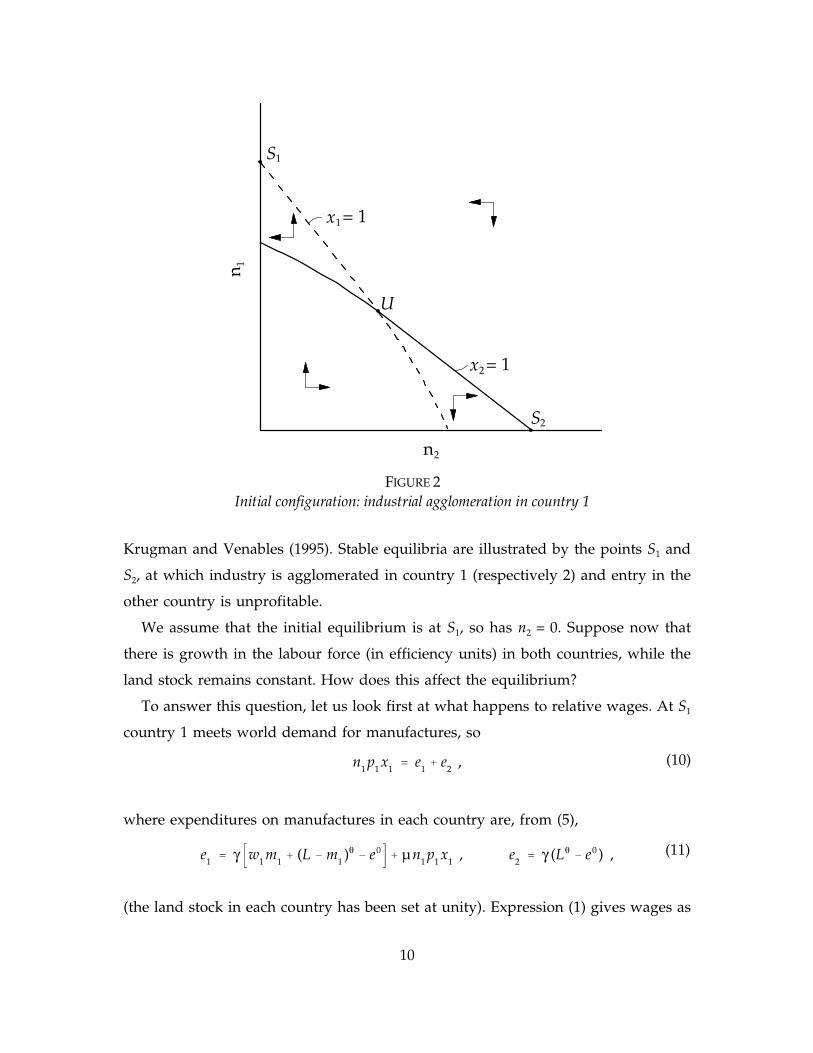
Krugman and Venables (1995). Stable equilibria are illustrated by the points S1 and
n2
n 1
U
S1
S2
x2 = 1
x1 = 1
FIGURE 2Initial configuration: industrial agglomeration in country 1
S2, at which industry is agglomerated in country 1 (respectively 2) and entry in the
other country is unprofitable.
We assume that the initial equilibrium is at S1, so has n2 = 0. Suppose now that
there is growth in the labour force (in efficiency units) in both countries, while the
land stock remains constant. How does this affect the equilibrium?
To answer this question, let us look first at what happens to relative wages. At S1
country 1 meets world demand for manufactures, so
(10)n1p
1x
1e
1e
2,
where expenditures on manufactures in each country are, from (5),
(11)e1
γ w1m
1(L m
1)θ e0 µn
1p
1x
1, e
2γ (Lθ e0 ) ,
(the land stock in each country has been set at unity). Expression (1) gives wages as
10
(12)w1
θ (L m1)(θ 1) , w
2θ L(θ 1) .
The country 1 manufacturing wage bill, w1m1 is a fraction (1 – µ) of the value of
output, e1 + e2, so, using (10)–(12),
(13)m1θ (L m
1)(θ 1) γ
1 γ(L m
1)θ Lθ 2e0 .
This equation gives country 1 manufacturing employment, m1, as a function of
parameters. Notice that if e0 is zero then the equation is homogenous of degree θ in
L and m1. However, if e0 is positive, then raising L raises m1 more than
proportionately, this increasing w1/w2:
(14)d(w
1/w
2)
dLγ 2e0 (1 θ)
Lθ [ (1 γ )(L θ m1) γ (L m
1)]
> 0 .
Turning to industry, at equilibrium S1 the price indices of expression (2) reduce to
(15)q1
n 1/(1 σ)1
p1
, q2
n 1/(1 σ)1
p1τ .
Demand for the output of each firm in country 1, and for a potential deviant locating
in 2 are, by (6) and (15),
(16)x1
e1
e2
n1p
1
1, x2
p2
p1
σ
e1τ (1 σ) e
2τ (σ 1)
n1p
1
,
and relative prices can be derived from (7) and (15) as
(17)
p2
p1
τ µ
w2
w1
(1 µ)
.
We have so far assumed that industry is agglomerated in country 1. Is this an
equilibrium? Yes, if the sales of a potential deviant locating in country 2 are less than
the level required to break even, i.e., if x2 < 1 at equilibrium S1. Substituting (17) in
(16) and eliminating n1 p1, we can express x2 as
11
(18)x2
w1
w2
σ (1 µ)
τ 1 σ σ µ
1e
2
e1
e2
τ 2(σ 1) 1 ,
where the share of country 2 in expenditure, derived from expressions (10)–(12), is
(19)e
2
e1
e2
γ (1 µ)(Lθ e0 )w
1m
1
.
If L is close to (e0)1/θ then total demand for manufactures is very low, wages in the
two countries are very close, and x2 is less than unity. There is then an equilibrium
at S1, as we illustrated it on figure 2. As L grows the forces at work can be seen from
equations (14), (18) and (19). Growth of L raises manufacturing employment in
country 1 and raises relative wages, equation (14), this increasing x2 through the first
term on the right hand side of (18). Pulling in the opposite direction, growth of L
reduces the share of country 2 in world expenditure for the product, because wage
differences mean that country 1’s consumer expenditure on manufactures is rising
relative to country 2’s. This means that the demand linkage is being strengthened, and
has the effect of reducing x2 (see equation (18), in which τ2(σ - 1) – 1 > 0). The net effect
is to increase x2, although it is not necessarily the case that limL → ∞(x2) > 1.
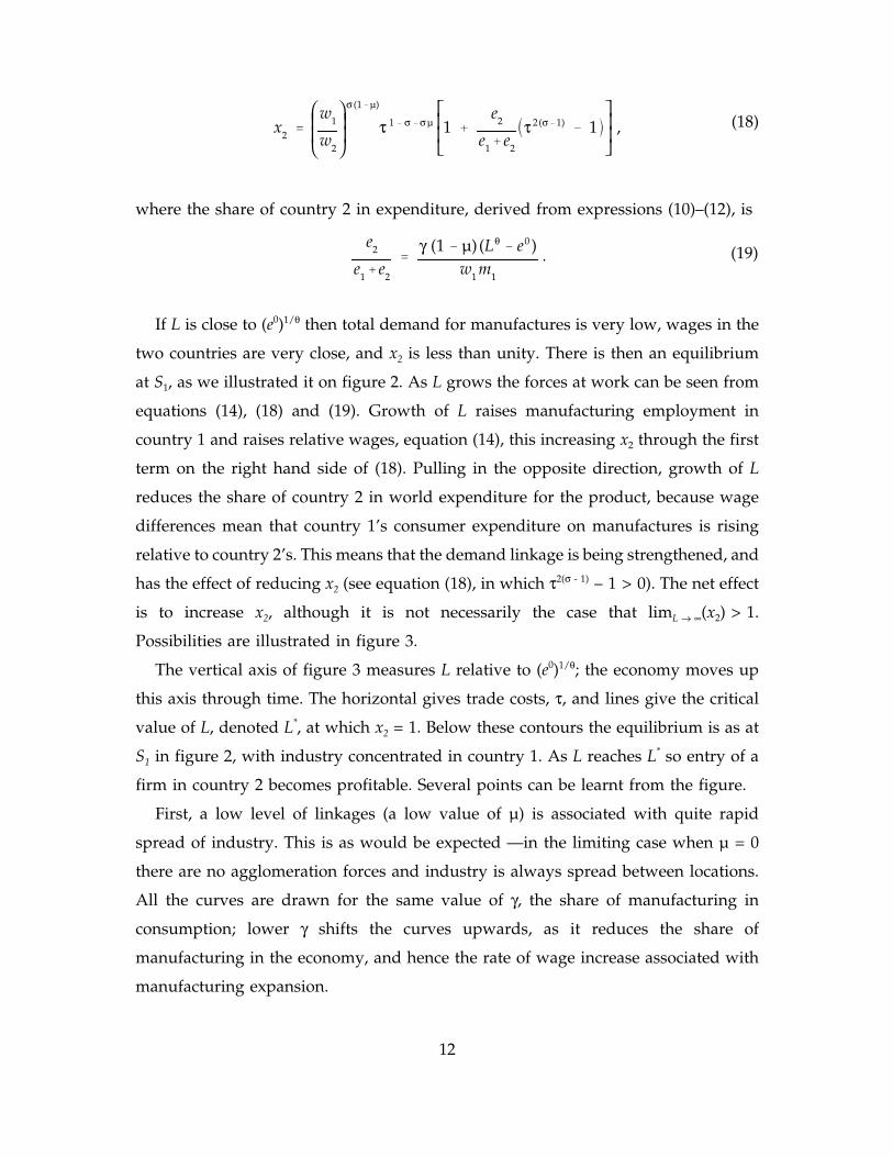
Possibilities are illustrated in figure 3.
The vertical axis of figure 3 measures L relative to (e0)1/θ; the economy moves up
this axis through time. The horizontal gives trade costs, τ, and lines give the critical
value of L, denoted L*, at which x2 = 1. Below these contours the equilibrium is as at
S1 in figure 2, with industry concentrated in country 1. As L reaches L* so entry of a
firm in country 2 becomes profitable. Several points can be learnt from the figure.
First, a low level of linkages (a low value of µ) is associated with quite rapid
spread of industry. This is as would be expected —in the limiting case when µ = 0
there are no agglomeration forces and industry is always spread between locations.
All the curves are drawn for the same value of γ, the share of manufacturing in
consumption; lower γ shifts the curves upwards, as it reduces the share of
manufacturing in the economy, and hence the rate of wage increase associated with
manufacturing expansion.
12
Second, the spread of industry is faster at high or low levels of trade barriers, τ,
FIGURE 3Values of L at which industrial production in country 2 becomes profitable
1 1.2 1.4 1.6 1.81
2
3
4
5
τ
L
µ 0.25=
µ 0.35=
*
(e )
0θ
1//
µ 0.45=µ 0.45=
than at intermediate levels. This is because when trade barriers are very high industry
must be divided between locations to meet final consumer demand. At the other
extreme, when barriers are very low, it only takes very small factor price differences
to induce relocation. It is a general property of models of this type that agglomeration
forces are strongest at intermediate barriers (see for examples Venables, 1996), and
this is what we see in the bell shape of the curves in figure 3.
Third, it is possible that as L goes to infinity industry remains concentrated in
location 1 (this occurring in this example if µ exceeds 0.48). Agglomeration may
therefore remain an equilibrium if µ is high, τ takes an intermediate value, and there
is a low share of manufactures in demand, γ.
We have demonstrated that when L reaches L* entry of a manufacturing firm in
country 2 is profitable. What then happens as L increases further?
In terms of figure 2, the spread of industry comes as follows. Growth in L shifts
both the zero profit contours upwards, but the x2 = 1 locus shifts faster, coming to
13
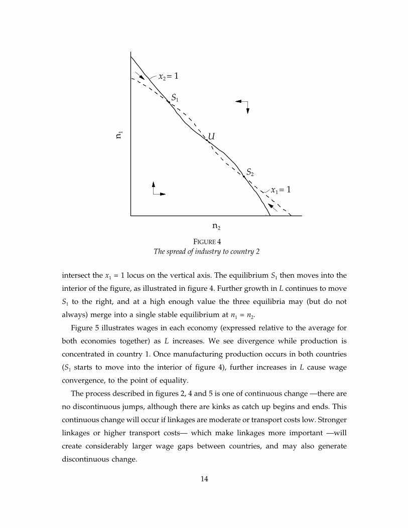
intersect the x1 = 1 locus on the vertical axis. The equilibrium S1 then moves into the
n2
n 1 U
S1
S2
x1= 1
x2 = 1
FIGURE 4The spread of industry to country 2
interior of the figure, as illustrated in figure 4. Further growth in L continues to move
S1 to the right, and at a high enough value the three equilibria may (but do not
always) merge into a single stable equilibrium at n1 = n2.
Figure 5 illustrates wages in each economy (expressed relative to the average for
both economies together) as L increases. We see divergence while production is
concentrated in country 1. Once manufacturing production occurs in both countries
(S1 starts to move into the interior of figure 4), further increases in L cause wage
convergence, to the point of equality.
The process described in figures 2, 4 and 5 is one of continuous change —there are
no discontinuous jumps, although there are kinks as catch up begins and ends. This
continuous change will occur if linkages are moderate or transport costs low. Stronger
linkages or higher transport costs— which make linkages more important —will
create considerably larger wage gaps between countries, and may also generate
discontinuous change.
14
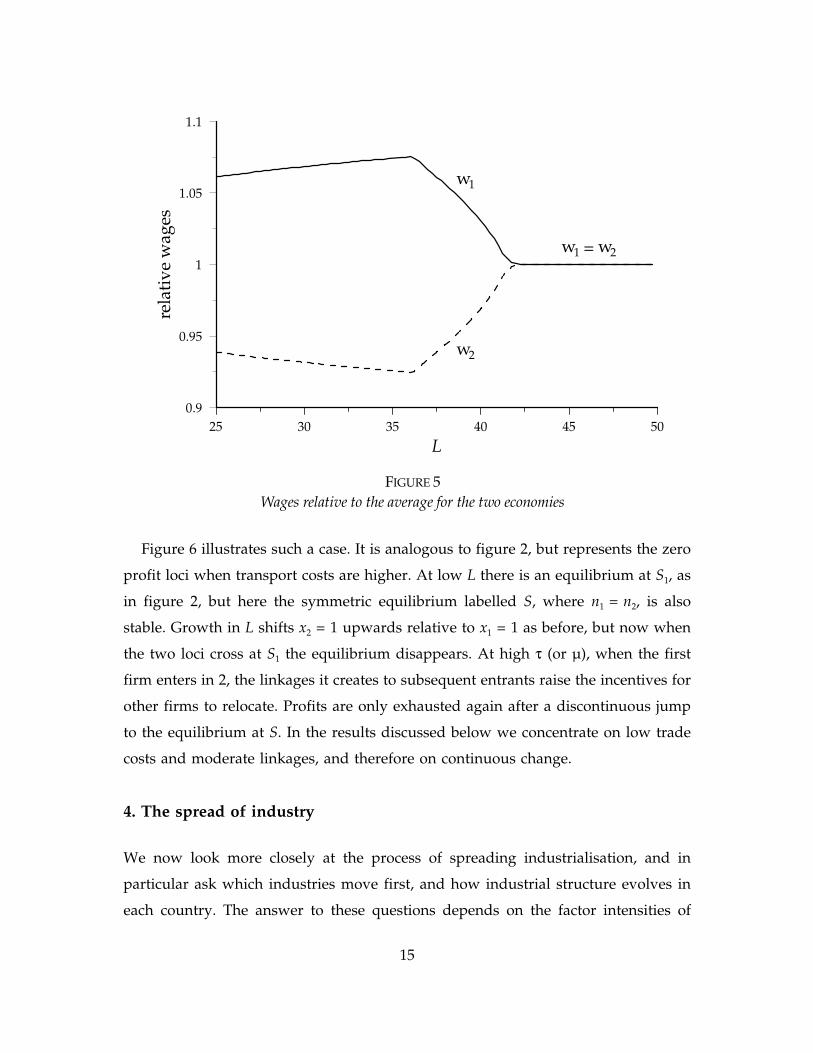
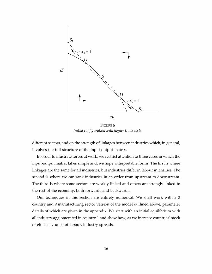
Figure 6 illustrates such a case. It is analogous to figure 2, but represents the zero
Wages relative to the average for the two economiesFIGURE 5
25 30 35 40 45 500.9
0.95
1
1.05
1.1
L
rela
tive
wag
esw1
w2
w2w1 =
profit loci when transport costs are higher. At low L there is an equilibrium at S1, as
in figure 2, but here the symmetric equilibrium labelled S, where n1 = n2, is also
stable. Growth in L shifts x2 = 1 upwards relative to x1 = 1 as before, but now when
the two loci cross at S1 the equilibrium disappears. At high τ (or µ), when the first
firm enters in 2, the linkages it creates to subsequent entrants raise the incentives for
other firms to relocate. Profits are only exhausted again after a discontinuous jump
to the equilibrium at S. In the results discussed below we concentrate on low trade
costs and moderate linkages, and therefore on continuous change.
4. The spread of industry
We now look more closely at the process of spreading industrialisation, and in
particular ask which industries move first, and how industrial structure evolves in
each country. The answer to these questions depends on the factor intensities of
15
different sectors, and on the strength of linkages between industries which, in general,
n2
n 1
S
S1
S2
x2 = 1
x1 = 1
U
U
Initial configuration with higher trade costsFIGURE 6
involves the full structure of the input-output matrix.
In order to illustrate forces at work, we restrict attention to three cases in which the
input-output matrix takes simple and, we hope, interpretable forms. The first is where
linkages are the same for all industries, but industries differ in labour intensities. The
second is where we can rank industries in an order from upstream to downstream.
The third is where some sectors are weakly linked and others are strongly linked to
the rest of the economy, both forwards and backwards.
Our techniques in this section are entirely numerical. We shall work with a 3
country and 9 manufacturing sector version of the model outlined above, parameter
details of which are given in the appendix. We start with an initial equilibrium with
all industry agglomerated in country 1 and show how, as we increase countries’ stock
of efficiency units of labour, industry spreads.
16
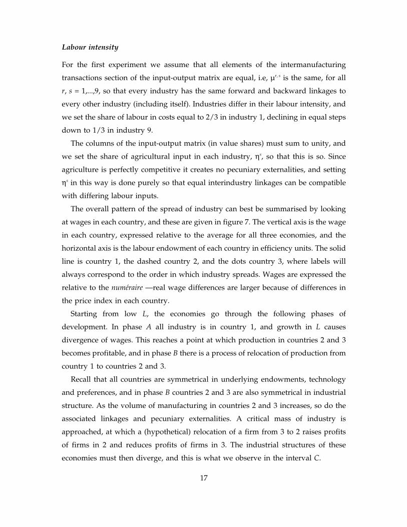
Labour intensity
For the first experiment we assume that all elements of the intermanufacturing
transactions section of the input-output matrix are equal, i.e, µr, s is the same, for all
r, s = 1,...,9, so that every industry has the same forward and backward linkages to
every other industry (including itself). Industries differ in their labour intensity, and
we set the share of labour in costs equal to 2/3 in industry 1, declining in equal steps
down to 1/3 in industry 9.
The columns of the input-output matrix (in value shares) must sum to unity, and
we set the share of agricultural input in each industry, ηs, so that this is so. Since
agriculture is perfectly competitive it creates no pecuniary externalities, and setting
ηs in this way is done purely so that equal interindustry linkages can be compatible
with differing labour inputs.
The overall pattern of the spread of industry can best be summarised by looking
at wages in each country, and these are given in figure 7. The vertical axis is the wage
in each country, expressed relative to the average for all three economies, and the
horizontal axis is the labour endowment of each country in efficiency units. The solid
line is country 1, the dashed country 2, and the dots country 3, where labels will
always correspond to the order in which industry spreads. Wages are expressed the
relative to the numéraire —real wage differences are larger because of differences in
the price index in each country.
Starting from low L, the economies go through the following phases of
development. In phase A all industry is in country 1, and growth in L causes
divergence of wages. This reaches a point at which production in countries 2 and 3
becomes profitable, and in phase B there is a process of relocation of production from
country 1 to countries 2 and 3.
Recall that all countries are symmetrical in underlying endowments, technology
and preferences, and in phase B countries 2 and 3 are also symmetrical in industrial
structure. As the volume of manufacturing in countries 2 and 3 increases, so do the
associated linkages and pecuniary externalities. A critical mass of industry is
approached, at which a (hypothetical) relocation of a firm from 3 to 2 raises profits
of firms in 2 and reduces profits of firms in 3. The industrial structures of these
economies must then diverge, and this is what we observe in the interval C.
17
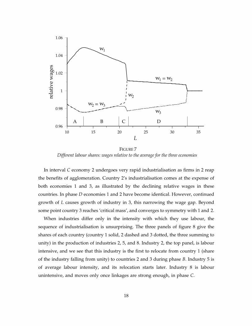
In interval C economy 2 undergoes very rapid industrialisation as firms in 2 reap
Different labour shares: wages relative to the average for the three economiesFIGURE 7
10 15 20 25 30 350.96
0.98
1
1.02
1.04
1.06
L
rela
tive
wag
esw1
w2
w2w1 =
w3w2 =w3
A B C D
the benefits of agglomeration. Country 2’s industrialisation comes at the expense of
both economies 1 and 3, as illustrated by the declining relative wages in these
countries. In phase D economies 1 and 2 have become identical. However, continued
growth of L causes growth of industry in 3, this narrowing the wage gap. Beyond
some point country 3 reaches ‘critical mass’, and converges to symmetry with 1 and 2.
When industries differ only in the intensity with which they use labour, the
sequence of industrialisation is unsurprising. The three panels of figure 8 give the
shares of each country (country 1 solid, 2 dashed and 3 dotted, the three summing to
unity) in the production of industries 2, 5, and 8. Industry 2, the top panel, is labour
intensive, and we see that this industry is the first to relocate from country 1 (share
of the industry falling from unity) to countries 2 and 3 during phase B. Industry 5 is
of average labour intensity, and its relocation starts later. Industry 8 is labour
unintensive, and moves only once linkages are strong enough, in phase C.
18
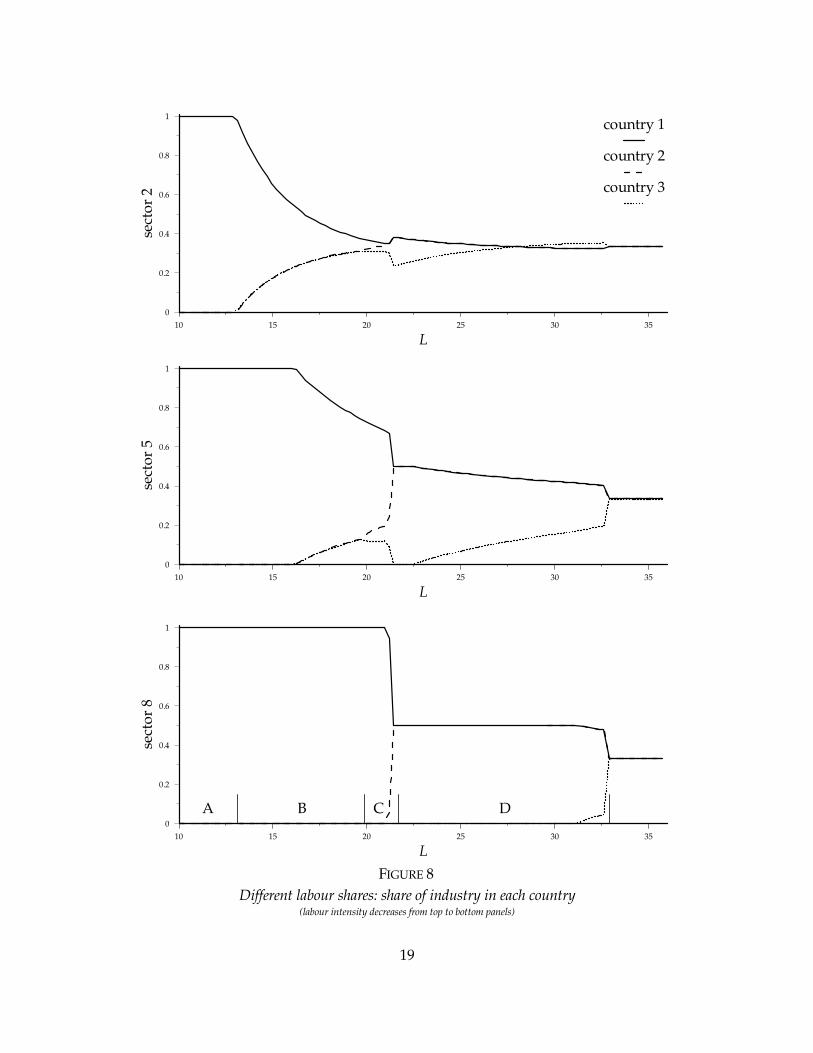
FIGURE 8Different labour shares: share of industry in each country
(labour intensity decreases from top to bottom panels)
10 15 20 25 30 35
0
0.2
0.4
0.6
0.8
1
L
sect
or 2
10 15 20 25 30 35
0
0.2
0.4
0.6
0.8
1
L
sect
or 8
10 15 20 25 30 35
0
0.2
0.4
0.6
0.8
1
L
sect
or 5country 1
country 2
country 3
A B C D
19
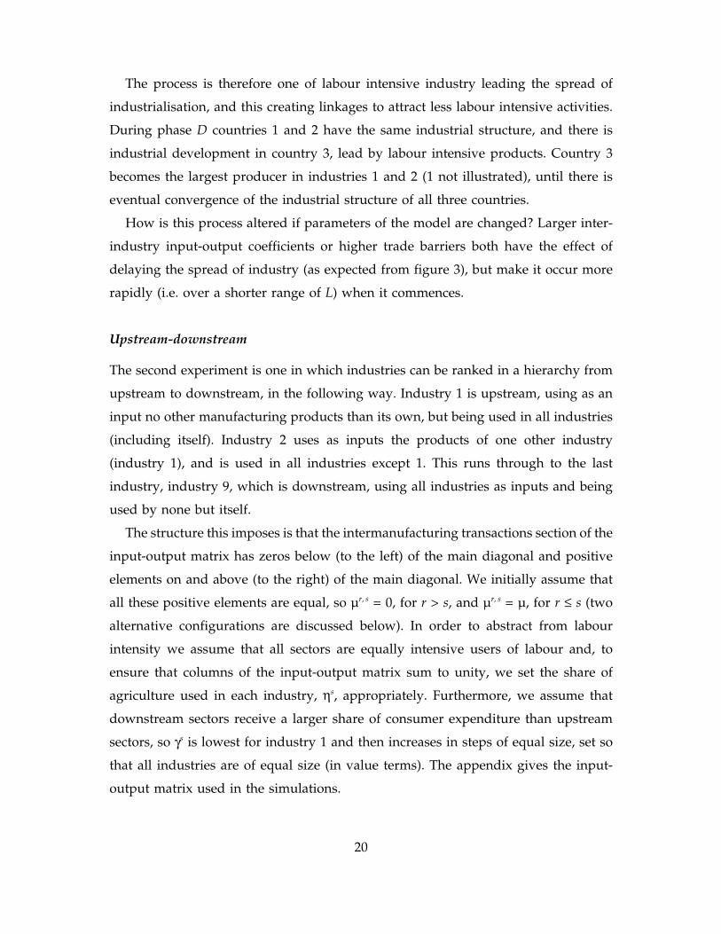
The process is therefore one of labour intensive industry leading the spread of
industrialisation, and this creating linkages to attract less labour intensive activities.
During phase D countries 1 and 2 have the same industrial structure, and there is
industrial development in country 3, lead by labour intensive products. Country 3
becomes the largest producer in industries 1 and 2 (1 not illustrated), until there is
eventual convergence of the industrial structure of all three countries.
How is this process altered if parameters of the model are changed? Larger inter-
industry input-output coefficients or higher trade barriers both have the effect of
delaying the spread of industry (as expected from figure 3), but make it occur more
rapidly (i.e. over a shorter range of L) when it commences.
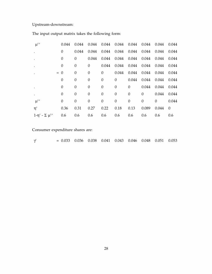
Upstream-downstream
The second experiment is one in which industries can be ranked in a hierarchy from
upstream to downstream, in the following way. Industry 1 is upstream, using as an
input no other manufacturing products than its own, but being used in all industries
(including itself). Industry 2 uses as inputs the products of one other industry
(industry 1), and is used in all industries except 1. This runs through to the last
industry, industry 9, which is downstream, using all industries as inputs and being
used by none but itself.
The structure this imposes is that the intermanufacturing transactions section of the
input-output matrix has zeros below (to the left) of the main diagonal and positive
elements on and above (to the right) of the main diagonal. We initially assume that
all these positive elements are equal, so µr, s = 0, for r > s, and µr, s = µ, for r ≤ s (two
alternative configurations are discussed below). In order to abstract from labour
intensity we assume that all sectors are equally intensive users of labour and, to
ensure that columns of the input-output matrix sum to unity, we set the share of
agriculture used in each industry, ηs, appropriately. Furthermore, we assume that
downstream sectors receive a larger share of consumer expenditure than upstream
sectors, so γs is lowest for industry 1 and then increases in steps of equal size, set so
that all industries are of equal size (in value terms). The appendix gives the input-
output matrix used in the simulations.
20
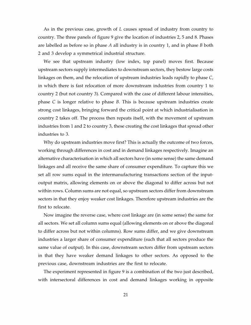
As in the previous case, growth of L causes spread of industry from country to
country. The three panels of figure 9 give the location of industries 2, 5 and 8. Phases
are labelled as before so in phase A all industry is in country 1, and in phase B both
2 and 3 develop a symmetrical industrial structure.
We see that upstream industry (low index, top panel) moves first. Because
upstream sectors supply intermediates to downstream sectors, they bestow large costs
linkages on them, and the relocation of upstream industries leads rapidly to phase C,
in which there is fast relocation of more downstream industries from country 1 to
country 2 (but not country 3). Compared with the case of different labour intensities,
phase C is longer relative to phase B. This is because upstream industries create
strong cost linkages, bringing forward the critical point at which industrialisation in
country 2 takes off. The process then repeats itself, with the movement of upstream
industries from 1 and 2 to country 3, these creating the cost linkages that spread other
industries to 3.
Why do upstream industries move first? This is actually the outcome of two forces,
working through differences in cost and in demand linkages respectively. Imagine an
alternative characterisation in which all sectors have (in some sense) the same demand
linkages and all receive the same share of consumer expenditure. To capture this we
set all row sums equal in the intermanufacturing transactions section of the input-
output matrix, allowing elements on or above the diagonal to differ across but not
within rows. Column sums are not equal, so upstream sectors differ from downstream
sectors in that they enjoy weaker cost linkages. Therefore upstream industries are the
first to relocate.
Now imagine the reverse case, where cost linkage are (in some sense) the same for
all sectors. We set all column sums equal (allowing elements on or above the diagonal
to differ across but not within columns). Row sums differ, and we give downstream
industries a larger share of consumer expenditure (such that all sectors produce the
same value of output). In this case, downstream sectors differ from upstream sectors
in that they have weaker demand linkages to other sectors. As opposed to the
previous case, downstream industries are the first to relocate.
The experiment represented in figure 9 is a combination of the two just described,
with intersectoral differences in cost and demand linkages working in opposite
21
FIGURE 9Upstream-downstream: share of industry in each country
(upstream to downstream from top to bottom panels)
10 10.5 11 11.5 12 12.5
0
0.2
0.4
0.6
0.8
1
L
sect
or 2
10 10.5 11 11.5 12 12.5
0
0.2
0.4
0.6
0.8
1
L
sect
or 8
10 10.5 11 11.5 12 12.5
0
0.2
0.4
0.6
0.8
1
L
sect
or 5country 1
country 2
country 3
A B C D
22
directions. The combined effect in the experiment is that cost linkages are more
powerful than demand linkages, so upstream industries are the first to be detached
from country 1’s industrial complex, with downstream sectors rapidly following.
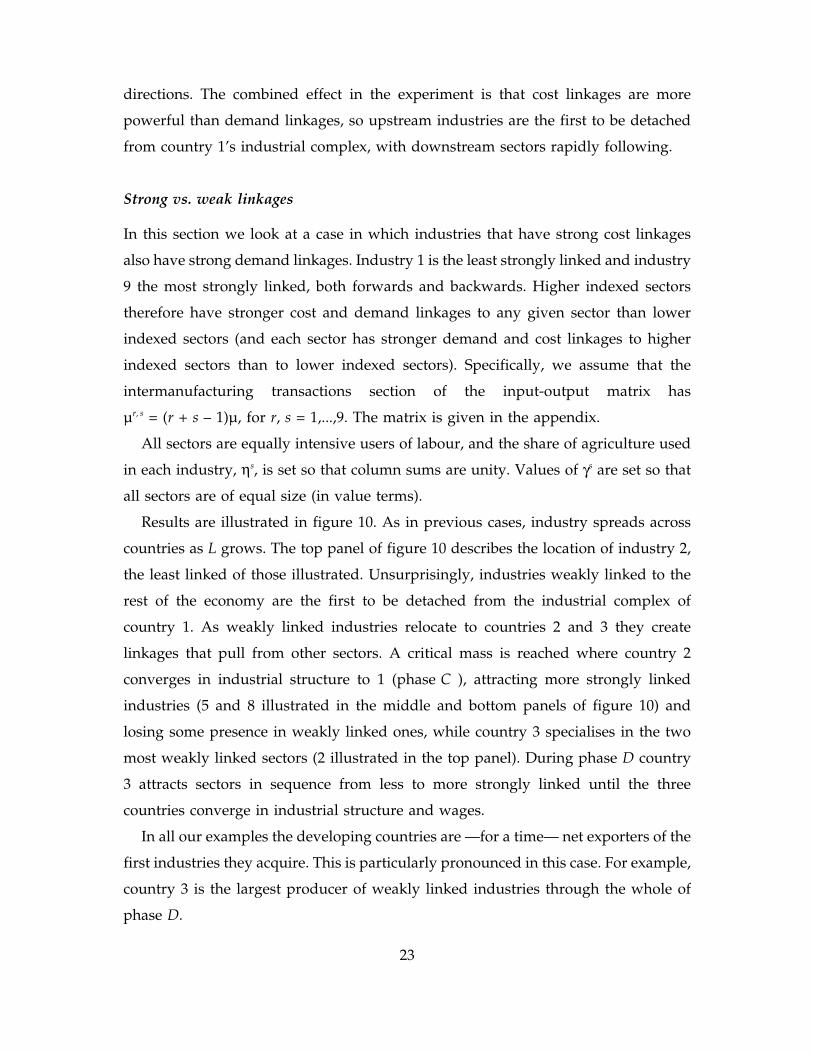
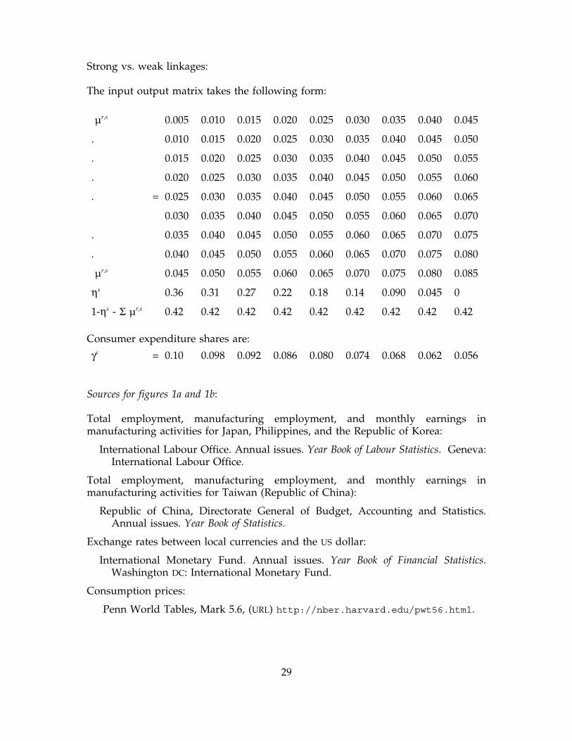
Strong vs. weak linkages
In this section we look at a case in which industries that have strong cost linkages
also have strong demand linkages. Industry 1 is the least strongly linked and industry
9 the most strongly linked, both forwards and backwards. Higher indexed sectors
therefore have stronger cost and demand linkages to any given sector than lower
indexed sectors (and each sector has stronger demand and cost linkages to higher
indexed sectors than to lower indexed sectors). Specifically, we assume that the
intermanufacturing transactions section of the input-output matrix has
µr, s = (r + s – 1)µ, for r, s = 1,...,9. The matrix is given in the appendix.
All sectors are equally intensive users of labour, and the share of agriculture used
in each industry, ηs, is set so that column sums are unity. Values of γs are set so that
all sectors are of equal size (in value terms).
Results are illustrated in figure 10. As in previous cases, industry spreads across
countries as L grows. The top panel of figure 10 describes the location of industry 2,
the least linked of those illustrated. Unsurprisingly, industries weakly linked to the
rest of the economy are the first to be detached from the industrial complex of
country 1. As weakly linked industries relocate to countries 2 and 3 they create
linkages that pull from other sectors. A critical mass is reached where country 2
converges in industrial structure to 1 (phase C ), attracting more strongly linked
industries (5 and 8 illustrated in the middle and bottom panels of figure 10) and
losing some presence in weakly linked ones, while country 3 specialises in the two
most weakly linked sectors (2 illustrated in the top panel). During phase D country
3 attracts sectors in sequence from less to more strongly linked until the three
countries converge in industrial structure and wages.
In all our examples the developing countries are —for a time— net exporters of the
first industries they acquire. This is particularly pronounced in this case. For example,
country 3 is the largest producer of weakly linked industries through the whole of
phase D.
23
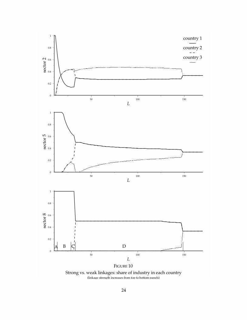
FIGURE 10Strong vs. weak linkages: share of industry in each country
(linkage strength increases from top to bottom panels)
50 100 1500
0.2
0.4
0.6
0.8
1
L
sect
or 2
50 100 1500
0.2
0.4
0.6
0.8
1
L
sect
or 8
50 100 1500
0.2
0.4
0.6
0.8
1
L
sect
or 5country 1
country 2
country 3
A B C D
24
5. Concluding comments
This paper provides a radical way of thinking about the process of industrialisation.
Interactions between imperfect competition, transport costs, and an input-output
structure create incentives for firms to locate close to supplier and customer firms.
Clustering of firms then occurs, so that even if countries are identical in underlying
structure, only a few countries are industrialised. These countries have high wages,
but the positive pecuniary externalities created by inter-firm linkages compensate for
the higher wage costs. An increase in demand for manufactures raises wages in
industrialised countries, leading to a point at which some firms choose to become
established in a new country. Industrialisation then commences in this country, and
takes place at a rapid rate as forward and backward linkages are created and a critical
mass of industry attained. The process may then repeat itself, so industrialisation
takes the form of a sequence of waves, with industry spreading from country to
country.
The process we describe abstracts from many important aspects of industrial
development. We have no capital accumulation (physical or human), no government,
and no international differences in technology. Even within its framework the model
we employ is simple; for example, firms are modelled as single plant operations, so
multinationality and foreign direct investment are not considered. Nevertheless, we
think the approach provides some new insights. It explains the rapid ‘take-off’ of
newly industrialising economies, and highlights the way in which industrial structure
may change during industrialisation.
The speed of the process, and which industries are the first to relocate, are
determined by the input-output structure, establishing the strength of forward and
backward linkages between industries as well as their factor intensity. So far we have
only looked at hypothetical input-output structures, which sacrifice empirical
foundations to isolate specific effects. We have learnt four things from them.
First, stronger linkages tie firms more tightly to existing agglomerations, and
therefore postpone the spread of industry and cause it to happen in a more abrupt
manner.
25
Second, labour intensive industries tend to leave first, as they are most affected by
increases in industrialised countries’ wages relative to the rest of the world. The
development of labour intensive activities makes it profitable for labour unintensive
sectors to follow, and when a critical mass is reached industrialisation can take off
rapidly.
Third, upstream industries face higher costs of market access when they move
away from an existing industrial cluster, but are not heavily dependent on proximity
of suppliers of intermediate inputs. This suggests that upstream industries tend to
leave early, and have a significant effect in pulling downstream industries along in
their wake. However, different structures of the input-output matrix can create cases
where demand is more important, and downstream industries move first.
Finally, weakly linked industries benefit less from being close to other industries
(they neither sell a large fraction of their output to other industries nor spend a large
share of their costs on intermediates produced by them). They are therefore the first
to relocate in response to labour cost differentials, being gradually followed by more
strongly linked industries.
26
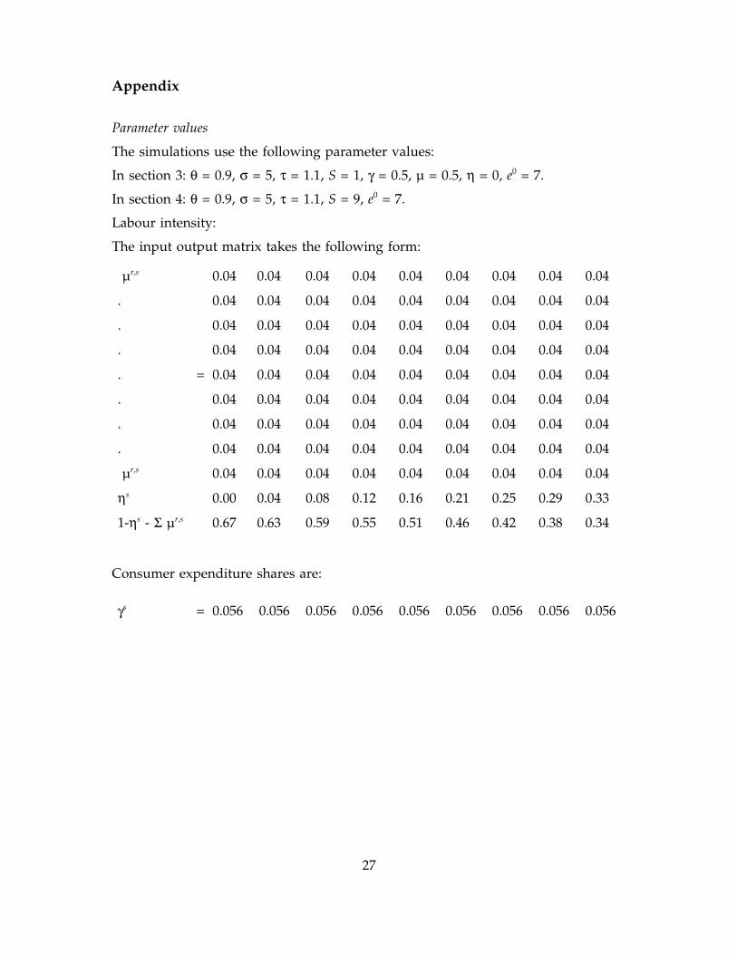
Appendix
Parameter values
The simulations use the following parameter values:
In section 3: θ = 0.9, σ = 5, τ = 1.1, S = 1, γ = 0.5, µ = 0.5, η = 0, e0 = 7.
In section 4: θ = 0.9, σ = 5, τ = 1.1, S = 9, e0 = 7.
Labour intensity:
The input output matrix takes the following form:
µr,s 0.04 0.04 0.04 0.04 0.04 0.04 0.04 0.04 0.04
. 0.04 0.04 0.04 0.04 0.04 0.04 0.04 0.04 0.04
. 0.04 0.04 0.04 0.04 0.04 0.04 0.04 0.04 0.04
. 0.04 0.04 0.04 0.04 0.04 0.04 0.04 0.04 0.04
. = 0.04 0.04 0.04 0.04 0.04 0.04 0.04 0.04 0.04
. 0.04 0.04 0.04 0.04 0.04 0.04 0.04 0.04 0.04
. 0.04 0.04 0.04 0.04 0.04 0.04 0.04 0.04 0.04
. 0.04 0.04 0.04 0.04 0.04 0.04 0.04 0.04 0.04
µr,s 0.04 0.04 0.04 0.04 0.04 0.04 0.04 0.04 0.04
ηs 0.00 0.04 0.08 0.12 0.16 0.21 0.25 0.29 0.33
1-ηs - Σ µr,s 0.67 0.63 0.59 0.55 0.51 0.46 0.42 0.38 0.34
Consumer expenditure shares are:
γs = 0.056 0.056 0.056 0.056 0.056 0.056 0.056 0.056 0.056
27
Upstream-downstream:
The input output matrix takes the following form:
µr,s 0.044 0.044 0.044 0.044 0.044 0.044 0.044 0.044 0.044
. 0 0.044 0.044 0.044 0.044 0.044 0.044 0.044 0.044
. 0 0 0.044 0.044 0.044 0.044 0.044 0.044 0.044
. 0 0 0 0.044 0.044 0.044 0.044 0.044 0.044
. = 0 0 0 0 0.044 0.044 0.044 0.044 0.044
0 0 0 0 0 0.044 0.044 0.044 0.044
. 0 0 0 0 0 0 0.044 0.044 0.044
. 0 0 0 0 0 0 0 0.044 0.044
µr,s 0 0 0 0 0 0 0 0 0.044
ηs 0.36 0.31 0.27 0.22 0.18 0.13 0.089 0.044 0
1-ηs - Σ µr,s 0.6 0.6 0.6 0.6 0.6 0.6 0.6 0.6 0.6
Consumer expenditure shares are:
γs = 0.033 0.036 0.038 0.041 0.043 0.046 0.048 0.051 0.053
28
Strong vs. weak linkages:
The input output matrix takes the following form:
µr,s 0.005 0.010 0.015 0.020 0.025 0.030 0.035 0.040 0.045
. 0.010 0.015 0.020 0.025 0.030 0.035 0.040 0.045 0.050
. 0.015 0.020 0.025 0.030 0.035 0.040 0.045 0.050 0.055
. 0.020 0.025 0.030 0.035 0.040 0.045 0.050 0.055 0.060
. = 0.025 0.030 0.035 0.040 0.045 0.050 0.055 0.060 0.065
0.030 0.035 0.040 0.045 0.050 0.055 0.060 0.065 0.070
. 0.035 0.040 0.045 0.050 0.055 0.060 0.065 0.070 0.075
. 0.040 0.045 0.050 0.055 0.060 0.065 0.070 0.075 0.080
µr,s 0.045 0.050 0.055 0.060 0.065 0.070 0.075 0.080 0.085
ηs 0.36 0.31 0.27 0.22 0.18 0.14 0.090 0.045 0
1-ηs - Σ µr,s 0.42 0.42 0.42 0.42 0.42 0.42 0.42 0.42 0.42
Consumer expenditure shares are:
γs = 0.10 0.098 0.092 0.086 0.080 0.074 0.068 0.062 0.056
Sources for figures 1a and 1b:
Total employment, manufacturing employment, and monthly earnings inmanufacturing activities for Japan, Philippines, and the Republic of Korea:
International Labour Office. Annual issues. Year Book of Labour Statistics. Geneva:International Labour Office.
Total employment, manufacturing employment, and monthly earnings inmanufacturing activities for Taiwan (Republic of China):
Republic of China, Directorate General of Budget, Accounting and Statistics.Annual issues. Year Book of Statistics.
Exchange rates between local currencies and the US dollar:
International Monetary Fund. Annual issues. Year Book of Financial Statistics.Washington DC: International Monetary Fund.
Consumption prices:
Penn World Tables, Mark 5.6, (URL) http://nber.harvard.edu/pwt56.html.
29
References
Dixit, Avinash K. and Joseph E. Stiglitz. 1977. ‘Monopolistic competition and optimumproduct diversity.’ American Economic Review, 67: 297–308.
Krugman, Paul R. and Anthony J. Venables. 1995. ‘Globalization and the inequalityof nations.’ Quarterly Journal of Economics, 110: 857-880.
Little, Ian. 1994. ‘Trade and industrialisation revisited.’ Pakistan Development Review,33: 359–389.
Rodrik, Dani. 1995. ‘Getting interventions right: how South Korea and Taiwan grewrich.’ Economic Policy, 20: 54–107.
Venables, Anthony J. 1996. ‘Equilibrium locations of vertically linked industries.’International Economic Review, 37: 341-359.
Young, Alwyn. 1995. ‘The tyranny of numbers: Confronting the statistical realities ofthe East Asian growth experience.’ Quarterly Journal of Economics, 110: 641–680.
30