Embed Size (px)
Citation preview

Urban Transport Expansions, Employment Decentralization, and
the Spatial Scope of Agglomeration Economies�
Nathaniel Baum-Snow, University of Toronto
February, 2017
Abstract
Using planned portions of the U.S. highway system as a source of exogenous variation, this
paper demonstrates that each new radial highway displaced 16% of central city working residents
but only 6% of jobs to the suburbs in the 1960-2000 period. In the context of a calibrated model
of urban structure, the implied elasticity of central city TFP to central city employment relative
to suburban employment is 0.02-0.05, meaning that a large fraction of overall agglomeration
economies operate at spatial scales below the metropolitan area level. Finance, insurance and
real estate exhibits the strongest such localized agglomeration spillovers and wholesale/retail
trade the weakest. Each highway causes central city income net of commuting costs to increase
by up to 3.6% and housing cost to decline by up to 3.0%. Factor reallocation toward land in
housing production generates the plurality of population decentralization with new highways.
�I thank Je¤rey Brinkman, Edward Glaeser, Esteban Rossi-Hansberg, William Strange and especially Lara Tobinfor helpful comments. Guillermo Alves, Kailin Clarke and Jorge Peréz provided excellent research assistance. Thepaper has bene�ted from discussions at numerous seminars and conferences. The author appreciates generous �nancialsupport from the Brown University Population Studies and Training Center.

1 Introduction
A large literature, including Ellison & Glaeser (1997), Rosenthal & Strange (2003), Duranton &
Overman (2005), Arzhagi & Henderson (2008), Ellison, Glaeser & Kerr (2010) and Billings &
Johnson (2016), uses observed spatial distributions of �rms and employment to draw conclusions
about the implied strength of agglomeration spillovers at very local spatial scales. Related papers
use plausibly exogenous sources of variation in �rm location incentives to recover information
about agglomeration economies in speci�c settings such as the siting of new large industrial plants
(Greenstone et al., 2010) and the rise and fall of the Berlin Wall (Ahlfeldt et. al, 2015). A di¤erent
literature, including Baum-Snow (2007), Duranton & Turner (2012) and Allen & Arkolakis (2014),
examines how transport infrastructure in�uences the spatial distribution of population within and
between cities and evaluates the social rate of return to interregional highways.
This paper uses estimated treatment e¤ects of radial urban highways on the allocations of jobs
and resident workers between central cities and suburbs of U.S. metropolitan areas to recover esti-
mates of parameters that govern productivity spillovers that operate below metro area spatial scales
and of components of the welfare consequences of new highways in the context of a quantitative
model. Highway treatment e¤ects are recovered using planned portions of the highway system as a
source of exogenous variation, as in Baum-Snow (2007), coupled with newly organized information
from 1960 and 2000 on spatial distributions of employment and resident worker locations by in-
dustry within metropolitan areas. The model is speci�ed with a geography that facilitates the use
of estimated treatment e¤ects and standard calibrated housing demand and production function
parameters as inputs. The welfare analysis incorporates the potential for new highways to in�uence
agglomeration spillovers both within and between cities and their surrounding suburbs because of
the exogenous shifts to �rm and residential location incentives that come with reduced commuting
costs.
Estimates indicate that while each radial highway displaced 16 percent of central city working
residents to suburbs, only 6 percent of jobs were displaced. This statistically signi�cant di¤erence
amounts to greater residential than employment decentralization in absolute terms for each new
highway, even with the initial higher concentration of employment in central cities. Greater e¤ects
of highways on residential than job location are also found in each broad industry category. Among
large private sector industries, wholesale & retail trade exhibits the highest employment location
response to new highways while �nance, insurance and real estate (FIRE) exhibits the lowest. The
smaller amount of variation in estimates across industries for workers� residential locations than
employment locations is an indication of variation in the strength of local agglomeration economies
across industries.
Relative magnitudes of agglomeration spillovers within versus between metropolitan area sub-
regions are quanti�ed using estimated treatment e¤ects of highways on employment location and
calibrated cost and expenditure share parameters. Results indicate that the elasticity of central
city total factor productivity (TFP) with respect to central city employment is at least 0.02 to
0.05 greater than the elasticity of central city TFP with respect to suburban employment, ceteris
1

paribus. This calculation follows directly from �rms� spatial indi¤erence condition, which says
that the strength of localized agglomeration economies must compensate for wage and land rental
cost di¤erences across locations, as mediated by cost shares. As commuting costs fall, central
city wage and rent premiums over the suburbs also fall, thereby requiring the central city TFP
premium to fall as well. Calibrated changes in relative TFP implied by changes in relative costs are
compared to estimated employment location responses to back out the relative productivity e¤ects
of employment within versus across metropolitan sub-regions. As in Roback (1982) and Albouy
(2016), these quantitative conclusions only depend on spatial indi¤erence conditions and do not
require imposing land market clearing or considering residential location choices. Central to the
analysis is that metropolitan area population is held constant. This allows for maintaining focus on
productivity impacts of spatial reorganization of a �xed population due to new highways without
having to consider population growth e¤ects simultaneously.
The estimated range of relative agglomeration spillovers indicate that most or all of the overall
metropolitan area level elasticity of TFP with respect to population is driven by sub-metropolitan
area scale interactions. Combes & Gobillon (2015) summarize consensus estimates of 0.04-0.07 for
elasticities of TFP with respect to metropolitan area population. Consistent with evidence in Baum-
Snow & Pavan (2012), estimates in this paper call into question the possibility that mechanisms for
agglomeration economies that operate at metropolitan area spatial scales, like labor market pooling,
are its important drivers. While in principle calibration of the model can also deliver quantitative
estimates of absolute levels of agglomeration spillovers in the central city and suburbs, in addition to
their relative levels, doing so requires imposing additional structure on the model. Agglomeration
parameter levels would be identi�ed mostly o¤ of structural assumptions rather than primarily o¤
of variation in �rm location choices that are induced by exogenous commuting cost reductions.
As such, it seems more sensible to reference the literature, which uses more appropriate models
and sources of identifying variation, for estimates of these metropolitan area scale agglomeration
parameters.
Calibrations of the full model reveal that each radial highway generates real income increases
of up to 3.6 percent and housing cost declines of up to 3.0 percent for central city residents, while
central city land rents decline by 4.3 to 12.8 percent with each radial highway. About half of the
real income increases occur because new highways open up additional urban space for productive
use, increasing land-labor ratios, while most of the remainder comes because of direct productivity
e¤ects of reduced intra-urban travel times. Finally, despite the importance of local agglomeration
spillovers for in�uencing �rm location choices, such spillovers explain only a small part of residential
location responses to new highways. About half of the decentralization caused by each highway ray
comes through reallocation toward land in housing production.
To summarize, this paper moves the literature forward in three directions. First, it provides
the �rst estimates of the causal e¤ects of highways on the spatial organization of economic activity
by industry within metropolitan areas, examining employment and residential location responses
simultaneously. Second, it is the �rst to employ exogenous shocks to the environment in a large set
2
of cities to facilitate recovery of productivity spillovers that operate at sub-metropolitan area spatial
scales. Third, as a complement to Duranton & Turner (2012) who calculate welfare e¤ects of new
highways associated with metropolitan area population changes, this is the �rst paper to quantify
the welfare bene�ts of new highways that accrue through various mechanisms in the context of an
environment in which population and employment is constrained to only move within an urban
area.
2 Data and Descriptive Evidence
2.1 Data on Worker and Job Location
Primary outcomes of interest are constructed using journey to work tabulations from the 1960 and
2000 censuses and 1960 census tract data coupled with digitized maps of 1960 geography central
cities and metropolitan areas. Commuting �ows by industry within and between central cities, 1960
de�nition standard metropolitan statistical area (SMSA) remainders and other regions for each of
the 100 largest SMSAs nationwide are reported in the journey to work supplement of the 1960
Census of Population. I aggregate this information into counts of workers and working residents
for central cities and SMSA remainders. Unfortunately, the 1960 census does not in most cases
report data in a way that makes it possible to break out such information for di¤erent central
cities. Therefore, all central cities in SMSAs with multiple central cities are necessarily treated as
one spatial unit. For the 78 fully tracted large SMSAs in 1960, I also construct counts of residents
by location and commuting �ows to the primary central city.1
For 2000, the Census Transportation Planning Package (CTPP) reports counts of workers and
working residents by industry for various small geographic units. It also reports the total count of
commuters between all pairs of these microgeographic units nationwide.2 This analysis maintains
the 1960 de�nition central city and SMSA geographies over time. In order to do this, digital
maps of 1960 central cities and SMSAs were created so that year 2000 census units could be
spatially allocated.3 Year 2000 microgeographic units of tabulation, typically tra¢ c analysis zones,
but census block groups or census tracts in some states, were allocated to 1960 geographies and
analogous counts were calculated through spatial aggregation.
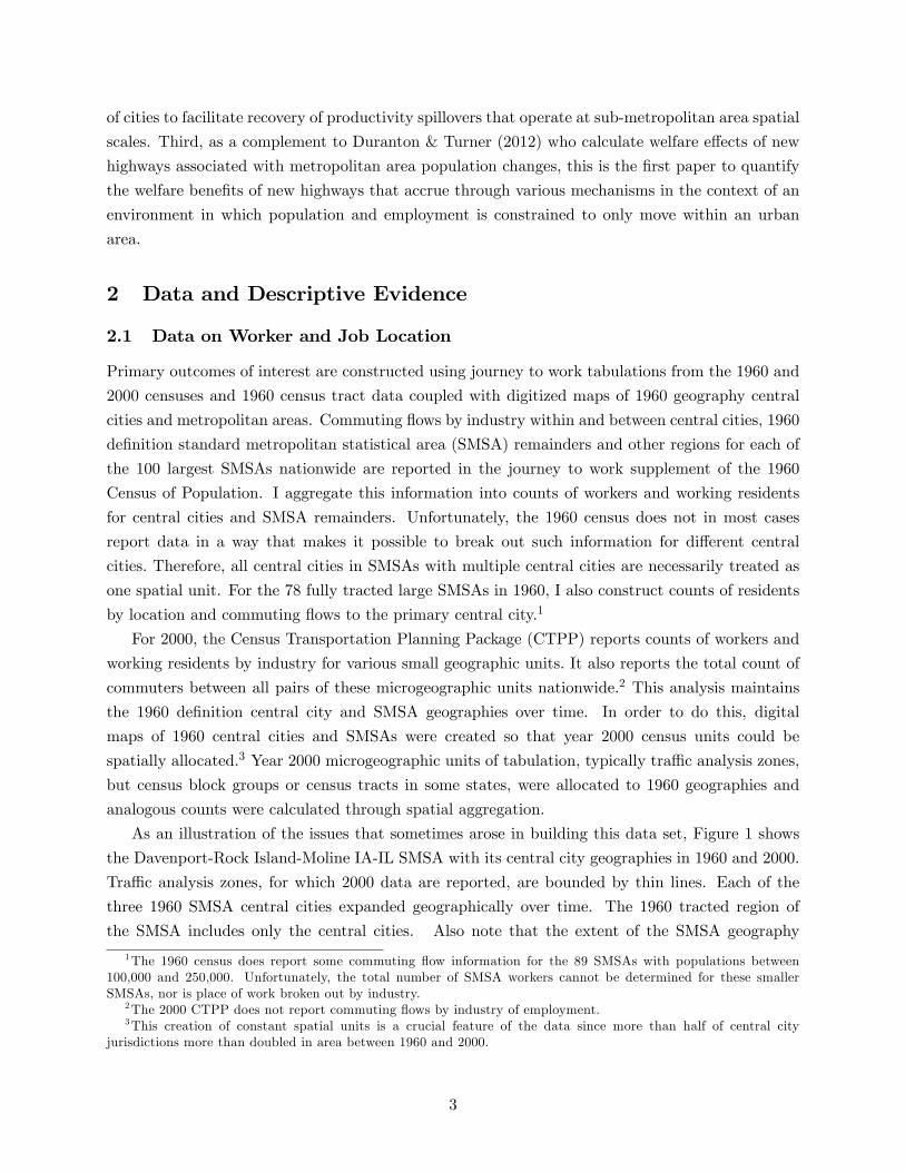
As an illustration of the issues that sometimes arose in building this data set, Figure 1 shows
the Davenport-Rock Island-Moline IA-IL SMSA with its central city geographies in 1960 and 2000.
Tra¢ c analysis zones, for which 2000 data are reported, are bounded by thin lines. Each of the
three 1960 SMSA central cities expanded geographically over time. The 1960 tracted region of
the SMSA includes only the central cities. Also note that the extent of the SMSA geography
1The 1960 census does report some commuting �ow information for the 89 SMSAs with populations between100,000 and 250,000. Unfortunately, the total number of SMSA workers cannot be determined for these smallerSMSAs, nor is place of work broken out by industry.
2The 2000 CTPP does not report commuting �ows by industry of employment.3This creation of constant spatial units is a crucial feature of the data since more than half of central city
jurisdictions more than doubled in area between 1960 and 2000.
3
is somewhat constrained. For this reason, I �nd it important to make use of information about
commutes into and out of each SMSA for the analysis, as is described in more detail below.
2.2 Decentralization of Working Residents, Employment and Commutes
Baum-Snow (2007a) documents that population decentralization out of central cities occurred in
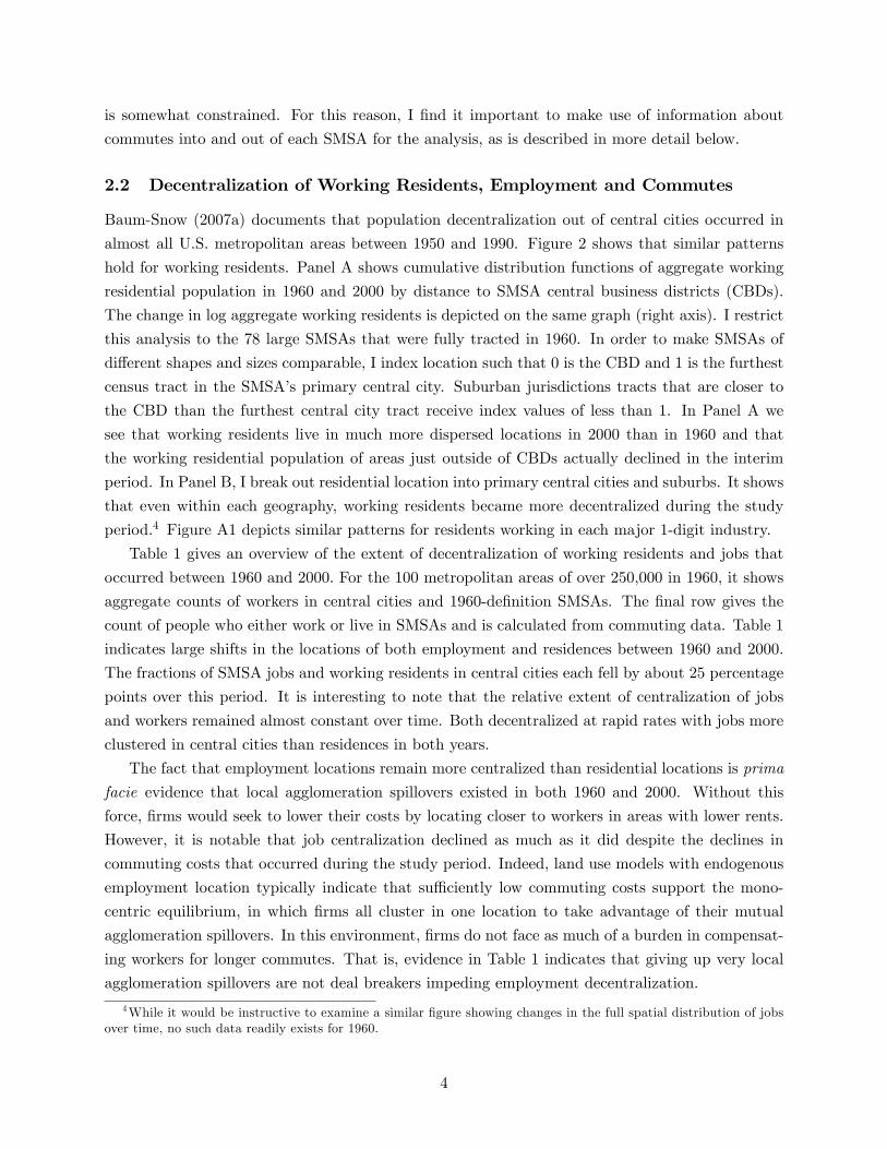
almost all U.S. metropolitan areas between 1950 and 1990. Figure 2 shows that similar patterns
hold for working residents. Panel A shows cumulative distribution functions of aggregate working
residential population in 1960 and 2000 by distance to SMSA central business districts (CBDs).
The change in log aggregate working residents is depicted on the same graph (right axis). I restrict
this analysis to the 78 large SMSAs that were fully tracted in 1960. In order to make SMSAs of
di¤erent shapes and sizes comparable, I index location such that 0 is the CBD and 1 is the furthest
census tract in the SMSA�s primary central city. Suburban jurisdictions tracts that are closer to
the CBD than the furthest central city tract receive index values of less than 1. In Panel A we
see that working residents live in much more dispersed locations in 2000 than in 1960 and that
the working residential population of areas just outside of CBDs actually declined in the interim
period. In Panel B, I break out residential location into primary central cities and suburbs. It shows
that even within each geography, working residents became more decentralized during the study
period.4 Figure A1 depicts similar patterns for residents working in each major 1-digit industry.
Table 1 gives an overview of the extent of decentralization of working residents and jobs that
occurred between 1960 and 2000. For the 100 metropolitan areas of over 250,000 in 1960, it shows
aggregate counts of workers in central cities and 1960-de�nition SMSAs. The �nal row gives the
count of people who either work or live in SMSAs and is calculated from commuting data. Table 1
indicates large shifts in the locations of both employment and residences between 1960 and 2000.
The fractions of SMSA jobs and working residents in central cities each fell by about 25 percentage
points over this period. It is interesting to note that the relative extent of centralization of jobs
and workers remained almost constant over time. Both decentralized at rapid rates with jobs more
clustered in central cities than residences in both years.
The fact that employment locations remain more centralized than residential locations is prima
facie evidence that local agglomeration spillovers existed in both 1960 and 2000. Without this
force, �rms would seek to lower their costs by locating closer to workers in areas with lower rents.
However, it is notable that job centralization declined as much as it did despite the declines in
commuting costs that occurred during the study period. Indeed, land use models with endogenous
employment location typically indicate that su¢ ciently low commuting costs support the mono-
centric equilibrium, in which �rms all cluster in one location to take advantage of their mutual
agglomeration spillovers. In this environment, �rms do not face as much of a burden in compensat-
ing workers for longer commutes. That is, evidence in Table 1 indicates that giving up very local
agglomeration spillovers are not deal breakers impeding employment decentralization.
4While it would be instructive to examine a similar �gure showing changes in the full spatial distribution of jobsover time, no such data readily exists for 1960.
4

Table 2 examines the extent to which industries di¤er in their patterns of decentralization.
From left to right, one digit industries (the �nest detail for which 1960 data is available) are listed
in order of 1960 SMSA employment shares.5 Rows 5 through 8 of Table 2 report overall trends
in SMSA working residents and employment by industry between 1960 and 2000. They show that
manufacturing and retail/wholesale trade were declining industries while services and �nance, in-
surance and real estate were growing. More relevant to the current analysis is the comparison across
industries of relative decentralization rates of jobs and workers�residential locations. Comparisons
of numbers in Rows 2 and 4 reveal less variation in the changes in central city fraction of working
residents than jobs across industries. Perhaps this is not surprising, as workers in each industry
have experienced the same set of incentives (apart from potential di¤erential changes in job access)
to suburbanize. However, di¤erences between results in Row 4 from Row 2 provides some evidence
about the di¤erences across industries in the ease of decentralization.
As is discussed in Baum-Snow (2010), the primary process through which decentralization of
�rms and workers occurred was by the modal commute shifting from being entirely within central
cities to being entirely within suburban regions. Figure 3 presents plots of the average fraction
commuting to primary central cities in 1960 and 2000 as functions of residential location in the
same 78 SMSAs used to construct Figure 2 using the same location index. Whether examined for
SMSAs overall (Panel A) or with primary central cities broken out separately from suburbs (Panel
B), we see secular declines in the fraction of working residents commuting to central cities at all
residential locations. Figure A2 shows that very similar changes in commuting patterns also hold
for six individual large metropolitan areas.
Table 3 quanti�es the associated changes in commuting patterns for the full sample of 100 large
SMSAs. It shows that while 43 percent of SMSA workers or jobs involved commutes within central
cities in 1960, this share fell to just 16 percent by 2000. Over the same period, the fraction living
and working in the suburban ring rose from 28 percent to 42 percent of the total. The only types of
commutes with declining shares of the total were those within central cities and those from suburbs
to central cities. This evidence is consistent with declines in the types of agglomeration forces that
keep �rms in central cities. At 7 percent in 2000 and 6 percent in 1960, reverse commutes have had
a small stable market share. The empirical work will conclude that shifts in commuting costs are
unrelated to shifts in patterns of reverse commutes across SMSAs. Therefore, reverse commutes
are not emphasized in the model in Section 6.
The �nal two columns of Table 3 give average one-way commuting times by type of commute
in 2000. Unfortunately such data are not available in 1960 as the commute time question did not
appear until the 1980 census. Results show that the longest commutes other than those involving
crossing SMSA boundaries are traditional suburb-central city commutes, at 25 to 46 percent longer
(depending on weighting procedure) than within central city commutes, which took 27 minutes for
the average worker and 19 minutes when averaged across SMSAs. Within suburban ring commute
5Because of inconsistencies across census years in the classi�cation of di¤erent types of services, I am forced tocombine all services into one broad industry category in order to make valid comparisons between 1960 and 2000.
5

times are notably similar to within central city commute times, though workers presumably enjoy
a rent discount which ends up capitalized into lower wages. This commuting time data will be used
in Section 6 to help recover parameters in the model.
2.3 Highway Data
Counts of radial limited access highways serving primary central cities�central business districts in
1950, 1960 and 2000 is the primary treatment variable used.6 As in Baum-Snow (2007a), Michaels
(2008), Baum-Snow (2010) and Duranton & Turner (2012), there is an econometric concern that
highways were not allocated randomly to metropolitan areas. Instead, highway construction cer-
tainly responded to increases in commuting demand precipitated by metropolitan area population
and economic growth. In addition, Duranton & Turner (2012) provide evidence that the federal gov-
ernment bankrolled additional highways beyond those in pre-1956 plans for economically struggling
regions to achieve �scal redistribution and to stimulate their local economies.
To address such potential endogeneity concerns, I instrument for the number of radial highways
constructed prior to 2000 with the number in a 1947 plan of the interstate highway system. As is
discussed in more detail in Baum-Snow (2007a), this plan was developed by the federal Bureau of
Public Roads based on observed levels of intercity tra¢ c and defense needs to promote intercity
trade and national defense. This highway plan was explicitly not developed to facilitate commuting
(U.S. Department of Transportation, 1977, p. 277). While the 1960 geography central city area
and radius are signi�cantly positively correlated with the number of planned highways, neither
SMSA population growth prior to 1950 nor the 1940 share of SMSA employment in any 1-digit
industry signi�cantly predicts the number of planned highways. Regressions of planned rays on
this set of shares or 1940-1950 SMSA population growth yield p-values of greater than 0.2 for all
coe¢ cients. The coe¢ cient on 1950 SMSA population in such a regression is positive with a p-value
of 0.179 while that for central city radius is just 0.007. More important central cities were larger
in area and got allocated more planned highways as a result; other potential indicators of cities�
importance for a national network are highly enough correlated with this measure that they do not
independently matter. Virtually the entire planned system (and more) was constructed because
the federal government provided 90 percent matching funding to an initial 10 percent covered by
individual states. Since the federal funding stream did not begin until 1956, it is logical that prior
outcomes are not correlated with planned rays.
This compendium of evidence supports the contention that the plan is a valid instrument
for highway construction of the subsequently built interstate system conditional on a measure of
central city size and SMSA �xed e¤ects. Inclusion of central city radius in regressions throughout
this analysis controls for the fact that more important cities, which are also larger, received more
planned highways.7 Table A1 presents summary statistics about the highway and demographic data
6Additional counts of other types of highways were also recorded but are not extensively used due to di¢ cultiesin isolating exogenous variation in them.
7Robustness checks on a subset of the sample and outcomes presented below using central city geographies thatare arti�cially constructed to be the same size in all SMSAs reveals no independent e¤ect of politically de�ned central
6

used in this analysis. It shows that sampled metropolitan areas received an average of 2.7 radial
highways between 1950 and 2000, with 2.0 of these built after 1960. The mean number of planned
highways is 2.9. Because of the high cost of building highways to serve central business districts,
cities with may planned highways often consolidate them into fewer central arteries serving the
downtown core.8
There is some question as to the appropriate starting year for measuring highways. With
interstate highway construction begun at a rapid rate after the passage of federal legislation in
1956, many cities had planned, partially completed or just opened segments in 1960. It is unlikely
that SMSA spatial equilibria would have come close to fully responding to this new transport
infrastructure in such a short time. Indeed, evidence in Baum-Snow (2007a) indicates that about
two-thirds of the long run response of urban form to the highway system occurs within 20 years.
Therefore, the main analysis in this paper uses the number of new radial highways serving central
cities constructed between 1950 and 2000.
Results in Table 4 show that this decision on how to count highways is if anything conservative.
Table 4 presents �rst stage results of the e¤ects of planned radial highways on the number actually
built. Panel A shows results using 1950 as a base while Panel B presents results using 1960 as a
base. Included control variables in Column 3, which is the baseline speci�cation throughout the
paper, can be justi�ed by a typical land use model as in Lucas & Rossi-Hansberg (2002) or a more
spatially aggregated version of such a model, as in that developed in Section 5 below. The choice of
control variables does not in�uence �rst stage coe¢ cients on planned rays. With 1950 as the base
year, coe¢ cients on planned rays are between 0.47 and 0.53. Coe¢ cients of interest are smaller by
0.13 to 0.17 when 1960 is instead the base year. Additional inclusion of 1950 log SMSA population,
1940-1950 SMSA population growth and 1940 1-digit industry shares do not signi�cantly change
coe¢ cients on planned rays, nor are coe¢ cients on any of these variables statistically signi�cant
(not reported). Because planned rays coe¢ cients are smaller for 1960-2000 than for 1950-2000,
second stage estimates are always larger if 1960 is used as the base year. Given the potential
concern that the timing of highway construction may be endogenous to commuting demand, with
the highways with the largest treatment e¤ects built �rst, results in the remainder of the paper
use 1950 to 2000 radial highway construction as the endogenous variable of interest, even though
outcomes of interest are measured as of 1960 and 2000.
One other piece of evidence in Table 4 is relevant for helping to justify the empirical strategy
laid out in the following section. Inclusion of growth in the number of people who live or work in
the SMSA does not a¤ect the coe¢ cient on the instrument. As is discussed in more detail below,
this variable is included in the �rst stage in order to hold SMSA scale constant throughout the
analysis. In practice, inclusion of this control variable brings up potential endogeneity concerns.
city size on outcomes of interest, as should be expected.8 I also tried using the number of radial highways of various classes of priority serving each city in a 1922 federal war
department plan of the national highway system, the "Pershing Map", as instruments. This plan was put togetherwith less regard for intercity trade than the 1947 plan used to construct the instrument. Unfortunately, instrumentsderived from the Pershing Map are insu¢ ciently strong to be useful for this analysis.
7

However, conditioning on this variable has no e¤ect on results because it is not correlated with the
instrument. A regression of 1960-2000 SMSA population or employment growth in 1947 planned
radial highways and central city radius yields a small insigni�cant coe¢ cient of 0.014 (se=0.029).
This very small correlation between the instrument and SMSA growth means that true coe¢ cients
of interest can be estimated with very tight bounds, as is further explored in the following section.
3 Empirical Strategy
The primary empirical goal of this paper is to recover average treatment e¤ects of radial highways
on the decentralization of central city working residents and jobs in broad industry categories.
Because SMSA employment by industry may endogenously respond to the highway treatment, as in
Duranton & Turner (2012) and Duranton, Morrow & Turner (2013), it is important to explicitly hold
SMSA employment by industry constant. Rather than using log central city employment or working
residents by industry as dependent variables, it is tempting to conceptualize a neighborhood choice
model with Extreme Value Type I shocks, which would deliver log central city shares as dependent
variables of interest. Any estimated e¤ects of roads would then re�ect some combination of impacts
on decentralization and growth. Controlling for SMSA employment by industry on the right hand
side instead facilitates empirically isolating the e¤ects of roads on the allocation of employment
and resident workers between central cities and suburbs. The focus of this section is to show how
this is achieved in a practical way, while taking into account the potential endogeneity of SMSA
employment mix and scale to the highway treatment. As is discussed in the prior section, the
potential endogeneity of �hwy is addressed by instrumenting with the number of radial highways
in the 1947 national plan.
The objective is to estimate coe¢ cients in the following equations. In these equations, �1kand r1k describe causal e¤ects of highways on the allocations of employment empCCki and working
population popCCki in industry k and SMSA i between central cities and suburbs. Key here is to
hold SMSA employment or working population in industry k constant.
� ln empCCki = �0k + �1k�hwyi + �2k� ln empSMSAki +
Xj 6=k
�j2k� ln empSMSAji +Xi%k + �ki (1)
� ln popCCki = r0k + r1k�hwyi + r2k� ln popSMSAki +
Xj 6=k
rj2k� ln popSMSAji +XiRk + uki (2)
One challenge with recovering consistent estimates of parameters of interest �1k and r1k is the fact
that highways may not only cause decentralization, but they may also cause the industry mix to
change. That is, � ln empSMSAki and � ln popSMSA
ki may be endogenous, or correlated with the error
term, even after instrumenting for �hwyi with planned highways from 1947. This occurs because
� ln empSMSAki and � ln popSMSA
ki may themselves respond to the instrument, thereby violating
the standard exclusion restriction required for IV to provide consistent estimates. There are of
course additional identi�cation concerns in Equations (1) and (2). These are discussed below in the
8

context of equations whose parameters are actually estimated. A �nal potential di¢ culty is that
there may be cross-industry e¤ects. That is, for example, the total number of SMSA workers in
services may in�uence where manufacturing �rms locate. I provide some indirect evidence below
that such cross-industry e¤ects, as captured by �j2k and rj2k, are small.
To get around inclusion of industry-speci�c SMSA employment as predictors for identifying
parameters of interest �1k and r1k, I proceed in two steps. The �rst step generates estimates of the
e¤ects of highways on the mix of SMSA employment across industries. The results of this step are
interesting in their own right, but are not the focus of this analysis. Similar estimates have been
explored in existing research with more detailed and appropriate data, as in Duranton, Morrow
& Turner (2013). The second step is to recover the reduced form e¤ects of highways on central
city employment and working residents by industry taking as given only the evolution of total
metropolitan area employment between 1960 and 2000. Combining estimates from these two steps
yields e¤ects of highways on this set of outcomes holding the evolution of total SMSA employment
by industry �xed. In practice, these two steps can be carried out simultaneously using GMM or
3SLS.
In step one of the empirical analysis, I consider regressions of the form:
� ln empSMSAki = �0k + �1k�hwyi + �2k� ln popemp
SMSAi +Xi�k + "ki (3)
� ln popSMSAki = a0k + a1k�hwyi + a2k� ln popemp
SMSAi +XiBk + eki (4)
Rather than using either SMSA employment or working population as controls, I instead control for
� ln popempSMSA, which is the change in the log of the number of people who either work or reside
(or both) in SMSA i. This allows any di¤erences in coe¢ cient estimates between (3) and (4) to
be uniquely attributable to the di¤erent outcomes. The control for � ln popempSMSA is necessary
for the coe¢ cients �1k and a1k to capture the e¤ects of highways on SMSA industry composition
rather than simply the level of employment in each industry. The reduced form causal e¤ects of
highways absent this control variable would partially re�ect the e¤ect on total SMSA population
or employment, overstating the e¤ect of highways holding SMSA scale constant. Xi is a vector of
additional control variables conditional on which the planned rays instrument is exogenous.
Several identi�cation concerns arise in estimating Equations (3) and (4). First is the endogeneity
of � lnhwy, which is addressed by instrumenting with the number of radial highways in the 1947
national plan. Second is the potential endogeneity of� ln popempSMSA. If highways are an amenity,
this object should respond positively to the number of highways, whether planned or built. On the
other hand, direct inclusion of � ln popempSMSA may introduce a correlation with the error term
since shocks to one sector of employment mechanically a¤ect aggregate employment in all sectors.
In practice, results in the next section indicate that the bias from excluding this control is small
since it does not respond much to highways.
If highways cause SMSA population growth, it can be shown that excluding � ln popempSMSAi
from (3) and (4) leads to transport coe¢ cients that are positively biased, whereas including this
9

variable yields transport coe¢ cients that are negatively biased. The econometrics of these biases
is seen in the following simpli�ed environment. Consistent with (3) and (4), suppose that the
underlying structural equations for SMSA jobs in each industry are
� ln empSMSAki = �0k + �1k�hwyi + �2k� ln popemp
SMSAi + "ki:
Here, �hwyi is instrumented with hwy47i , which is uncorrelated with "ki. An analogous vector of
equations describe the data generating process for SMSA working residents in each industry. The
probability limit of the IV estimate of �1k excluding �ln(popempSMSAi ) from the regression equals
�1k + �2kCov(hwy47;� ln popempSMSA)
Cov(�hwy; hwy47).
The probability limit of the IV estimate of �1k including this variable in the regression, as written
above, is
�1k �Cov(hwy47;� ln popempSMSA)Cov(� ln popempSMSA; "k)
D > 09.
That is, given that Cov(hwy47; ln popempSMSA) > 0, as is true in the data and is also found by
Duranton & Turner (2012), and Cov(ln popempSMSA; "k) > 0, as is true if unobservables driving
variation in ln empSMSAk also in�uence the total SMSA employment, excluding versus including the
control for metropolitan area scale bookends true highway rays coe¢ cients in (3) and (4). As an
alternative, one can instrument for � ln popempSMSA in addition to �hwy. Similar to Glaeser &
Gyourko (2005) and Saiz (2010), I use average January temperature and annual precipitation as
instruments in a robustness check, as these amenities are stronger relative consumer demand shifters
for living in SMSAs in 2000 than they were in 1960 because of improvements in climatization and
building technologies.10
An additional issue is to consider which variables belong in additional controls X. There are
two justi�cations for including variables in this control set. First, from an econometric perspective,
any variable correlated with the number of planned highways that may cause the SMSA industry
mix to change must be included for an IV estimator to yield consistent estimates of a1 and �1.
Second, in the estimation equations speci�ed below that describes changes in the allocation of
workers and jobs between central cities and suburbs, there are theoretical justi�cations to include
any exogenous variables that appear in a typical closed city land use model. Strictly speaking, given
an ideal instrument for highways that is unconditionally random, we would not need to include any
such variables. However, central city size is both model-relevant and correlated with planned rays,
and thus must be included as a control variable in regressions. Larger area central cities received
more planned highways and (all else equal) had less loss of population and jobs to the suburbs.
It should be noted that with ideal data in a world perfectly described by land use models,
10An alternative commonly used instrument for the growth in total metropolitan area employment or populationis Bartik (1991) style industry shift-shares. Such instruments are less suitable for this analysis since historicalindustry shares are likely to be mechanically correlated with unexplained components of 1960-2000 industry speci�cemployment changes.
10

Equations (3) and (4) would be identical. That is, conceptually we typically de�ne metropolitan
areas as commuting zones that are fully self-contained. In practice, as seen in Table 3, 8 percent of
SMSA workers or residents either lived or worked outside their SMSA in 1960, rising to 22 percent
by 2000. Use of data on all people who live or work in each SMSA is thus important, so that the
analysis is not arti�cially constrained by SMSA geographies. Results reported in the next section
will reveal that SMSA counts of jobs and working residents are su¢ ciently similar such that we
cannot statistically distinguish between estimates of �1k and a1k.
Armed with estimates of a1k and �1k, the next step is to specify equations that allow for
recovery the impacts of highways on urban decentralization by industry holding the SMSA industry
composition constant. In order to avoid including endogenous variables, I specify these equations as
the following "reduced forms" in which the prediction variables are exactly the same as in Equations
(3) and (4) and the outcomes are for 1960 de�nition central cities. Indeed, substitution of (3) and
(4) into (1) and (2) yields a pair of equations that resemble (5) and (6).
� ln empCCki = !0k + !1k�hwyi + !2k� ln popempSMSAi +XiDk +$ki (5)
� ln popCCki = w0k + w1k�hwyi + w2k� ln popempSMSAi +Xi�k + vki (6)
In estimating parameters of these equations, once again rays in the 1947 plan serve as an instrument
for �hwy and similar justi�cations hold for inclusion of additional control variables X. Arguments
for negative biases of !1k and w1k when including � ln popempSMSA in the regressions and positive
biases of these coe¢ cients when excluding � ln popempSMSA from these regressions hold as for (3)
and (4). In particular, since unobservables driving variation in outcomes are also likely to in�uence
� ln popempSMSA in the same direction, � ln popempSMSA is likely to be positively correlated with
the error terms. Weather variables again serve as instruments for � ln popempSMSA in robustness
checks.
Solving out from the reduced forms, the causal e¤ects of each highway on the decentralization of
jobs or working resident population by industry are given by the following expressions respectively:
�1k = !1k �!2k�2k
�1k +Xj 6=k(�1k�2k
�2j � �1j)�j2k (7)
r1k = w1k �w2ka2k
a1k +Xj 6=k(a1ka2ka2j � a1j)rj2k (8)
These expressions capture the intuition that the structural e¤ect of a highway on decentralization
within a given industry is the direct e¤ect on central city industry employment or working popula-
tion with one adjustment for the e¤ect on industry composition, whose size depends on highways�
in�uence on the importance of the industry in the economy, and an additional adjustment for cross-
industry e¤ects. Note that while �j2k and rj2k are not identi�ed, they are expected to be between
-1 and 1. Therefore, the terms capturing cross-industry e¤ects can be bounded. Moreover, the
cross-industry adjustment is expected to be smaller than the own-industry adjustment, which is
11

shown in the following section to be negligible except in manufacturing.
The following section discusses estimates of the four sets of elements used to build the ultimate
parameters of interest. Parameters can be recovered using linear IV equation by equation or GMM
or 3SLS on the systems of �ve equations given by (3), (4) (5), (6) and a "�rst stage" highways
equation estimated separately for each industry k.
4 Estimated Treatment E¤ects
4.1 E¤ects of Highways on SMSA Employment and Industry Mix
Table 5 reports regression results of Equations (3) and (4) in which planned highways enters as an
instrument for the total number of radial highways. Results in the �rst column reveal no evidence
of a signi�cant e¤ect of highways on total SMSA population or employment, though the point
estimate for total employment is slightly positive.11 The remaining columns of Table 5 show that
manufacturing is the only industry with a statistically signi�cant response of SMSA employment
to new transport infrastructure. Each radial highway is estimated to cause about 11 percent of the
manufacturing jobs and 14 percent of working residents to depart an SMSA, either to rural areas
or abroad.
While most rays coe¢ cients in Panel B are not statistically di¤erent from those in Panel A,
highways are estimated to cause greater declines in SMSA working residents than employment in
each industry. Gaps between rays coe¢ cients in Panel A and B range from 0.03 to 0.09 across
industries. In addition to its e¤ect on manufacturing, each highway is estimated to cause the
number of SMSA residents working in retail or wholesale trade to signi�cantly decline by 5 percent
and residents working in public administration to signi�cantly decline by 9 percent. Estimates
for other industries are not statistically signi�cant. The consistent discrepancy between highways
coe¢ cients in Panels A and B re�ects the residential decentralization out of 1960 de�nition SMSAs
caused by new highways.
Estimates in Table 5 are robust to various alternative speci�cations. As predicted by the bound-
ing argument given above, excluding � ln popempSMSA from industry-speci�c regressions always
increases rays coe¢ cients, with a maximum increase of 0.04 (for manufacturing employment and
working residents only) and in no cases changes statistical signi�cance of estimates. Instrument-
ing for � ln popempSMSA with weather variables changes rays coe¢ cients reported in Table 5 by
at most 0.01, though the joint �rst stage F-statistic falls from 16.75 to 5.30. No rays coe¢ cient
changes by more than 0.02 or is signi�cantly a¤ected by inclusion of a control for 1950 log SMSA
population except for total employment, which increases by 0.03 and military employment, which
11This result is in contrast to evidence in Baum-Snow (2007a) and Duranton & Turner (2012) that more highwaysled to metro area population increases. There are two reasons for this discrepancy. First, this paper uses moreconstrained metropolitan area geographies and much of the urban growth caused by highways manifested itself assprawl into outlying areas. Second, samples in the other two papers include many metropolitan areas that weresmaller than 250,000 in 1960. Point estimates for a subset of these smaller metropolitan areas also imply positivepopulation growth e¤ects of highways within 1960 SMSA geographies.
12
increases by 0.05. Additional inclusion of 1940 1-digit industry shares typically additionally in-
creases coe¢ cients, though not signi�cantly for any outcome. OLS regressions analogous to those
in Table 5 yield similar and statistically indistinguishable results for all outcomes except the num-
ber of resident workers in manufacturing. In industries for which they di¤er at all, OLS estimates
are slightly less negative than IV estimates, indicating that endogenously constructed highways had
smaller in�uences on the SMSA industry mix than their exogenous counterparts.
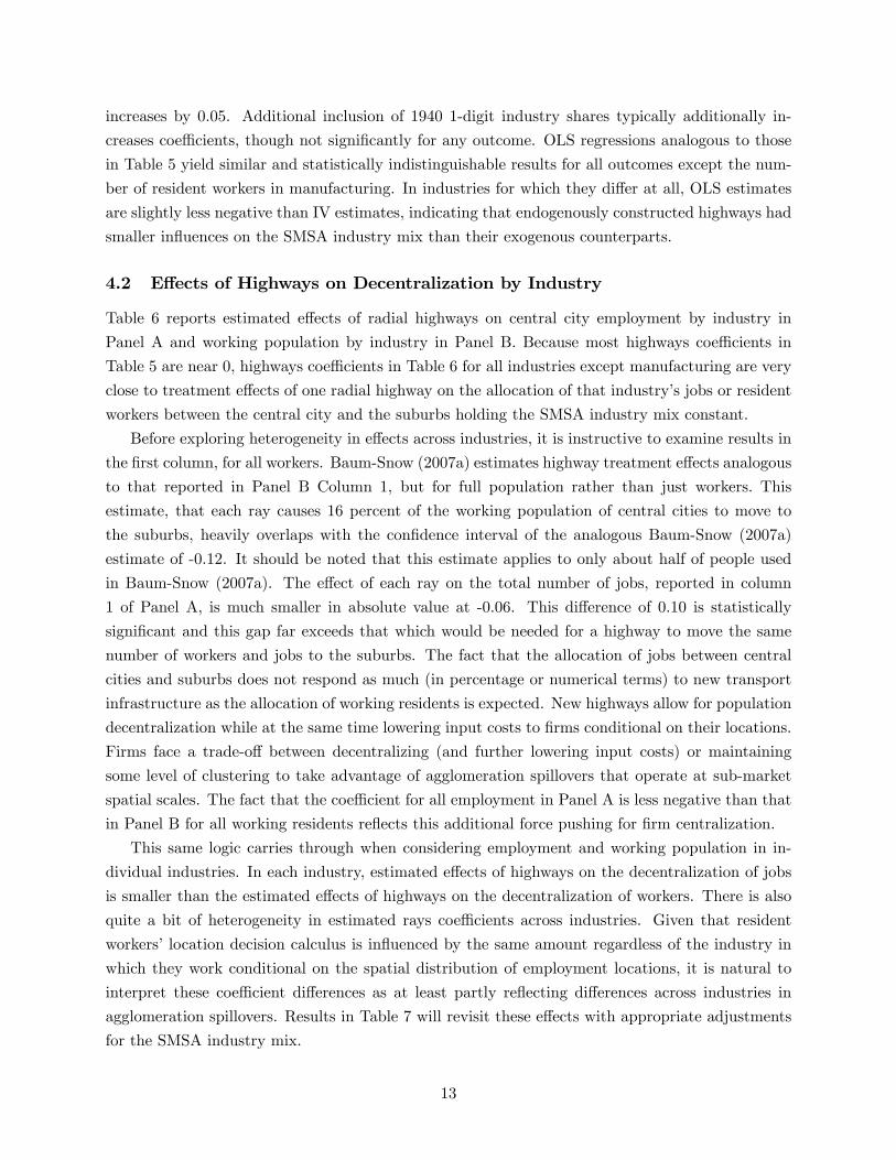
4.2 E¤ects of Highways on Decentralization by Industry
Table 6 reports estimated e¤ects of radial highways on central city employment by industry in
Panel A and working population by industry in Panel B. Because most highways coe¢ cients in
Table 5 are near 0, highways coe¢ cients in Table 6 for all industries except manufacturing are very
close to treatment e¤ects of one radial highway on the allocation of that industry�s jobs or resident
workers between the central city and the suburbs holding the SMSA industry mix constant.
Before exploring heterogeneity in e¤ects across industries, it is instructive to examine results in
the �rst column, for all workers. Baum-Snow (2007a) estimates highway treatment e¤ects analogous
to that reported in Panel B Column 1, but for full population rather than just workers. This
estimate, that each ray causes 16 percent of the working population of central cities to move to
the suburbs, heavily overlaps with the con�dence interval of the analogous Baum-Snow (2007a)
estimate of -0.12. It should be noted that this estimate applies to only about half of people used
in Baum-Snow (2007a). The e¤ect of each ray on the total number of jobs, reported in column
1 of Panel A, is much smaller in absolute value at -0.06. This di¤erence of 0.10 is statistically
signi�cant and this gap far exceeds that which would be needed for a highway to move the same
number of workers and jobs to the suburbs. The fact that the allocation of jobs between central
cities and suburbs does not respond as much (in percentage or numerical terms) to new transport
infrastructure as the allocation of working residents is expected. New highways allow for population
decentralization while at the same time lowering input costs to �rms conditional on their locations.
Firms face a trade-o¤ between decentralizing (and further lowering input costs) or maintaining
some level of clustering to take advantage of agglomeration spillovers that operate at sub-market
spatial scales. The fact that the coe¢ cient for all employment in Panel A is less negative than that
in Panel B for all working residents re�ects this additional force pushing for �rm centralization.
This same logic carries through when considering employment and working population in in-
dividual industries. In each industry, estimated e¤ects of highways on the decentralization of jobs
is smaller than the estimated e¤ects of highways on the decentralization of workers. There is also
quite a bit of heterogeneity in estimated rays coe¢ cients across industries. Given that resident
workers�location decision calculus is in�uenced by the same amount regardless of the industry in
which they work conditional on the spatial distribution of employment locations, it is natural to
interpret these coe¢ cient di¤erences as at least partly re�ecting di¤erences across industries in
agglomeration spillovers. Results in Table 7 will revisit these e¤ects with appropriate adjustments
for the SMSA industry mix.
13

As with the SMSA level regressions in Table 5, results in Table 6 are robust to a host of alterna-
tive speci�cations. Consistent with the bounding argument above, exclusion of � ln popempSMSA
from (5) and (6) increases the rays coe¢ cient for all outcomes except the residential locations of mil-
itary workers, but only by up to 0.03. Use of weather variables as instruments for � ln popempSMSA
a¤ects coe¢ cients of interest by less than 0.03 in all cases, except for military employment coe¢ -
cients which change by 0.03. Inclusion of 1950 log SMSA population and 1940 employment shares
in no case signi�cantly change rays coe¢ cients in Table 6.
Analogous OLS rays coe¢ cients reported in Table A2 are, with the exception of agricultural
and military employment, greater than their IV counterparts for all outcomes considered. As is
discussed in Baum-Snow (2007a), this discrepancy in part re�ects the fact that suburban highway
infrastructure likely matters for decentralization in addition to central city rays. In this case, IV and
OLS bound true treatment e¤ects since conditional on central city radius, the partial correlation
between central city and suburban ray construction is negative whereas the plan predicts positive
suburban ray construction. In addition, Duranton & Turner (2012) provide evidence that struggling
metropolitan areas were more likely to receive "endogenous" highways not predicted by the 1947
plan as a form of local economic development. Being less dynamic places growing at slower rates,
these metropolitan areas had fewer resources to build out and decentralize. Moreover, endogenous
highways were typically built later, connect to less suburban highway infrastructure and were lower
quality than planned highways, as most were constructed primarily with state and local funds.12
Thus, the actual treatment e¤ects of these highways is likely to be smaller in absolute value than
highways that are part of the national interstate system.13
I now examine the e¤ects of highways on the allocation of employment and working population
by industry between central cities and suburbs holding the industry mix strictly constant. Equations
(7) and (8) indicate the potential importance of adjusting the coe¢ cients reported in Table 6 for the
endogenous change in the industry mix induced by new highways in constructing such measures,
though evidence in Table 5 indicates that such changes are small in most industries. Table 7 reports
causal e¤ects of each radial highway on central city employment in Column 1 and resident workers
by industry in Column 2 holding the industry mix constant. Industry speci�c entries in Table 7 are
constructed by estimating a �ve equation system for each industry (including a "�rst stage") by
three-stage least squares and calculating causal e¤ects of interest using (7) and (8), ignoring any
potential cross-industry e¤ects. The delta method is used to calculate standard errors, with SMSA
clustering. Since own-industry SMSA employment composition adjustments are negligible for all
industries except manufacturing, and are small for manufacturing, any cross industry adjustments
to causal e¤ects of interest must be negligible.14
The �rst row of results in Table 7 is for all workers and matches up exactly to the �rst column
of Table 6, reiterating the headline estimated decentralization of 16 percent of central city residents
12The fact that the 1947 plan is a much stronger instrument for 1956-1960 highway construction than for 1956-2000highway construction, as seen in Table 4, indicates that highways built later were much more likely to be endogenous.13Attempts to precisely estimate nonlinear e¤ects of highways are unsuccessful because of large standard errors.14Estimating the same set of systems of equations by GMM yields almost identical results.
14

and 6 percent of central city employment caused by each radial highway. The second row also
applies to all workers but excludes the potentially endogenous control for � ln popempSMSAi in the
estimation equations. Commensurate with the result from Table 5 that highways had little e¤ect
on � ln popempSMSAi , these estimates are only 0.02 greater than those implied by the primary
speci�cation, at -0.04 for employment and -0.14 for residents. The bounding argument developed
in Section 3 above indicates that the true treatment e¤ects are between these two statistically
indistinguishable sets of numbers. Section 4.4 below further demonstrates robustness to exclusion
of � ln popempSMSAi as a control and to central city de�nition.
As the model developed in the following section demonstrates, magnitudes of employment re-
sponses to highways in di¤erent industries are directly related to strengths of localized agglomer-
ation economies provided the industry produces tradeable goods. Smaller e¤ects of highways on
employment decentralization are evidence of stronger agglomeration forces keeping �rms in the cen-
tral city. Estimated coe¢ cients on radial highways for central city employment in manufacturing,
services, TCPU and construction are about -0.08 and statistically signi�cant in most cases. Central
city employment in �nance insurance & real estate is estimated to decline by only about 4 percent
with each highway whereas employment in retail & wholesale trade declines by about 14 percent.
Evidence of associated relatively strong local agglomeration forces in �nance insurance & real estate
is quanti�ed more carefully in Section 6 using the model developed in Section 5. Because a large
component of output in wholesale and retail trade is not tradeable, it is natural that this industry�s
employment responses are more closely related to residential population responses to highways.
Central city employment in agriculture, public administration and the military have slightly posi-
tive estimated responses to highways. These are the industries in which the market probably has
the least in�uence on employment location. Except for manufacturing, industry speci�c treatment
e¤ect estimates are very similar to coe¢ cients in Table 6 because highways had only a small e¤ect
on the SMSA industry mix.
The second column of Table 7 presents causal e¤ects of each highway on central city working
residents by industry. These e¤ects exhibit much less variation across industries than do responses
of employment locations. Other than agriculture, which has a statistically insigni�cant treatment
e¤ect of -0.05, point estimates indicate that each highway caused between 12 and 21 percent of
central city workers to suburbanize, depending on industry. The smallest e¤ect is for workers in
�nance, insurance & real estate, which likely incorporates the relatively small response of �rm
location as well in this industry. The largest e¤ects are for those working in construction and
wholesale & retail trade. Gaps between e¤ects of highways on employment and residential locations,
reported in the third column of Table 7, are positive for each industry and statistically signi�cant
for many industries.
4.3 Commuting Mechanisms
Shifts in commuting patterns go along with the residential and employment decentralization e¤ects
of highways in Tables 6 and 7. Table 8 examines the e¤ects of radial highways on the eight types of
15

commuting �ows described in Table 3 using IV regression speci�cations analogous to those in the
�rst column of Table 6. These results indicate that highways had statistically signi�cant e¤ects on
three types of commuting �ows. Each highway caused 16 percent fewer commutes within central
cities, 11 percent more commutes within SMSA suburban rings and 22 percent more commutes
from outside of SMSAs to the suburban ring. Interestingly, the coe¢ cient estimate for traditional
suburb to central city commutes is not statistically signi�cant.15
Though they match up well to the resident worker population decentralization results in Tables
6 and 7, the commuting results may seem to be at odds with the much smaller estimated treatment
e¤ect of highways on central city employment. The following decomposition, in which r indexes
place of residence, helps in showing how these two sets of results can be reconciled:
� ln empCCi �X
r�fCC;ring;outgSemp
CC
ri � ln popr_empCCi .
The percent change in central city employment is the average of percent changes in the three types
of commuting �ow that involve working in the central city, weighted by their shares. The three
relevant dependent variables for this decomposition are in the �rst column of Table 8. Regressions
using the same dependent variables multiplied by 1960 shares, as indicated in the decomposition,
yield highway coe¢ cients of -0.10, 0.01 and 0.02 for central city, suburban ring and outside SMSA
residential locations respectively, adding up to -0.07. Only the last one is signi�cantly di¤erent from
its Table 8 counterpart. Discrepancies between these coe¢ cients from those in Table 8 are accounted
for by correlations between 1960 residential location shares for central city employees SempCC
ri and
the planned rays instrument conditional on central city radius and overall SMSA growth. Planned
rays signi�cantly predict the 1960 fraction living outside of an SMSA and working in the central
city conditional on controls, accounting for the signi�cant di¤erence with the result for this outcome
in Table 8. This highlights the importance of estimating results in di¤erences rather than levels,
thereby conditioning out �xed e¤ects that are correlated with the roads instrument.
One set of results in Table 8 is of note for conceptualizing a process that potentially generates
the data. While Table 3 shows that reverse commuting from central cities to suburbs rose relative to
other types of commuting �ows, results in Table 8 demonstrate that new highways cannot explain
this phenomenon. Instead, other changes in urban environments must be driving the rise in reverse
commuting. For example, increases in the relative consumer amenity values of cities versus suburbs
for some types of people (Couture & Handbury, 2016) may be one important explanation. Whatever
the explanations, because they are orthogonal to changes in commuting costs, such mechanisms
could not be central in the speci�cation of a model that focuses on understanding the e¤ects on
urban structure of reducing commuting costs.
15Similar regression results are reported in Baum-Snow (2010). While the two sets of results provide the samegeneral picture of commuting decentralization, they are not identical. There are two reasons for discrepancies. First,this paper uses all central cities whereas Baum-Snow (2010) uses just the primary central city. Second, Baum-Snow(2010) uses a broader sample of metropolitan areas.
16

4.4 Robustness to Speci�cation and Central City De�nition
To this point, I have necessarily de�ned central cities to correspond to their 1960 census geographies.
However, when examining e¤ects of highways on residential location, it is possible to rede�ne each
SMSA�s central city as being within a �xed radius of SMSA central business districts in tracted
SMSAs. While the limited availability of census tract data in 1960 reduces sample sizes to between
78 and 93 depending on CBD distance, I use such alternative central city geographies to demonstrate
that central city geographic de�nition does not drive the results in Tables 6 and 7. Figure 4 Panel
A graphs coe¢ cients on radial highways in regressions identical to those reported in Table 6 Panel
B Column 1 except that log central city working population for di¤erent central city radii are the
outcomes. If the central city radius is between 2 and 11 km from the CBD, each radial highway
is estimated to cause decentralization of 17 to 20 percent of central city resident workers. Beyond
11 km, the addition of each km in central city radius reduces the estimated e¤ect of each highway
by about 0.01. No coe¢ cient on true 1960 central city radius is statistically signi�cant in these
regressions. Also evident in Figure 4 is how similar coe¢ cients are when total SMSA working
population is excluded (top, blue line) versus included (bottom, red line) in the regression. Under
reasonable assumptions discussed in Section 4, true causal e¤ects of highways are bounded by these
two lines.
Figure 4 Panel B presents similar coe¢ cient estimates but when central city radius is determined
separately for each SMSA such that 10, 20, 30, 40 or 50 percent of SMSA employment in 2000 is
within the given radii, as calculated separately for each SMSA. The typical central city jurisdiction
hosted 34 percent of SMSA employment in 2000. This normalization indicates that the drift
upwards in coe¢ cient as a function of central city size seen in Panel A begins at radii below which
10 percent of employment is in the central city, for which each radial highway causes about 25
percent of central city working residents to move to the suburbs. The highways coe¢ cient levels
o¤ at -0.16 for radii containing 40-50 percent of year 2000 employment, which is the same estimate
reported in Table 6 Panel B. Figure A3 shows similar results using data from the larger sample of
154 SMSAs of over 100,000 in population in 1960 for which some 1960 census tract data exist.16
Unfortunately, an analogous exercise for job location is not possible because of data limitations
in 1960. Attempts to use data only from 2000 for such an exercise were unsuccessful and again
highlight the importance of �rst di¤erencing in order to control for unobserved �xed factors that
in�uenced allocations of planned highways.
5 Model
This section provides a framework for evaluating how the treatment e¤ects of transport improve-
ments on employment and population decentralization presented in the previous section can be
16Because of data limitations from 1960, it is not possible to include those who commute into SMSAs from outsidein the �ln popempi control used for Figure A3. This omission may explain the fact that rays coe¢ cients excludingthis control are slightly greater in absolute value, in contrast to the discussion in Section 4 and the results in Figure4.
17

used to recover information about the spatial scope of local agglomeration economies, mechanisms
through which highways drive urban population decentralization and welfare gains from new high-
ways. The model is su¢ ciently stylized such that comparative statics involving transport costs have
clear interpretations and the model can be calibrated with estimated treatment e¤ects along with
standard cost shares and housing demand parameters. Unlike many other land use models with
endogenous �rm location, this model is also simple enough such that it has a unique equilibrium
given transport cost and agglomeration forces.
To match the �xed population environment explored in the empirical work, this is a "closed
city" absentee landlord model with two metropolitan regions: the city and the suburbs. The
model is in the spirit of Rosen (1979) and Roback (1982) but with the addition of two types of
fundamental spillovers that exist between these two regions. First, there is commuting from the
suburbs to the city, allowing the number of residents not to equal the number of jobs. Second, there
are agglomeration spillovers between workers in the two regions which themselves may also depend
on the transportation cost. Because it is set up to be calibrated primarily using quantities rather
than prices, this model resembles Albouy & Stuart (2016) in some ways, though it considers the
spatial equilibrium within rather than between metropolitan areas.
The model is a spatially aggregated version of the land use models developed by Fujita &
Ogawa (1982) and Lucas & Rossi-Hansberg (2002), in which both �rm and residential locations
are endogenous in continuous space. Spatial delineation in the model mimics the nature of the
data used to recover treatment e¤ects explored in the previous section. Like its predecessors,
this model features no underlying worker or �rm heterogeneity. While such heterogeneity would
certainly be important for more richly characterizing equilibrium land use and commuting patterns,
it is immaterial for characterizing how such an equilibrium changes with reductions in commuting
costs. This is because textbook land use models with worker heterogeneity predict that the spatial
ordering of types does not change with secular declines in commuting costs. Empirically, the
spatial ordering of households by income has changed remarkably little since 1960. In 1960 and
2000 alike, average family or per-capita income in U.S. metropolitan areas increases with CBD
distance within central cities, levels o¤ in the suburbs and declines into rural portions of SMSAs
regardless of the strength of the highway treatment received (Baum-Snow & Lutz, 2011). Various
dimensions of unobserved heterogeneity, while not modeled explicitly, can thus be thought of as
being di¤erenced out via the exogenous highway shocks. Fu and Ross (2013) provide compelling
independent empirical evidence that worker heterogeneity does not drive productivity di¤erences
across space within metropolitan areas.
5.1 Setup
Workers and �rms compete for an exogenous amount of central city land Lc with market price
r per unit. The suburbs extend as far out as necessary to satisfy �rm and worker demand such
that there is no competition for space in the suburbs. As such, suburban land rent is determined
exogenously, and is denoted r. Of the exogenous population of the metropolitan area N , measure
18

Nc works in the city and measure Ns = N � Nc works in the suburbs. Qc is the total residentialpopulation of the city and Qs = N �Qc is the suburban residential population.
Central to model calibration is the time cost of commuting within the central city t, which is 0
for costless travel and 1 if it takes a worker�s full time endowment to make a round trip. Times for
commutes involving the suburbs are modeled as scalar multiples of t. To connect to the empirical
work, comparative statics will be evaluated with respect to t , as this is the variable for which we
have exogenous variation through the highway treatments. In particular, empirical estimates ofdNcdt and dQc
dt , calculated from regression results reported in Section 5, are used below as inputs to
model calibration.
5.1.1 The Tradeable Sector
Tradeable sector �rms produce the numeraire good using a constant returns to scale technology
with land, labor and capital. City �rms� total factor productivity incorporates a Hicks neutral
agglomeration force Ac(Nc; t) that is likely increasing in the total number of workers in the city
Nc in which the �rm is located. Because metro population is �xed, /Ac also implicitly depends on
suburban workers, where dAcdNcincorporates both the direct e¤ect of increases in Nc and the indirect
e¤ect of reductions in Ns. Productivity also depends negatively on the unit time cost of travel
t. For notational convenience, I also express suburban �rm TFP As(Nc; t) as depending on city
employment, where dAsdNc
is likely negative.
Because of the constant returns to scale technology, we can conceptualize each �rm as operating
on one unit of space. I denote nc as workers per unit space in the city and ns as workers per unit
space in the suburbs. kc and ks are capital per unit space in each region respectively. Labor,
capital and location are �rms�only choice variables. Pro�t functions for city and suburban �rms
respectively are thus:
�c = Ac(Nc; t)f(nc; kc)� r � wcnc � vkc�s = As(Nc; t)f(ns; ks)� r � wsns � vks:
In these expressions, wc and ws are wages and v is the capital rental rate, which does not di¤er
by location. Because �rms are fully mobile, they must earn the same pro�t in each location. Total
di¤erentiation of the indirect pro�t function given input costs yields the following equilibrium
relationship between productivity, wages and rents between the city and suburbs. This equation
is a within-metro version of one central Rosen (1979) and Roback (1982) equilibrium condition, in
which �N is the cost share of labor and �L is the cost share of land in production.
d lnA = �Nd lnw + �Ld ln r (9)
This equation indicates that the higher wage and rent location (the city) must also have higher total
factor productivity in order for �rms to be willing to locate there simultaneously as in the lower
cost suburbs. Because capital has the same cost in both locations, it drops out of this equation.
19

Optimization over the labor and capital inputs while imposing 0 pro�ts pins down the number
of workers hired at each �rm and the equilibrium wage. For these calculations, I employ the
Cobb-Douglas production technology f(n; k) = n k�. The central city wage as a function of rent
is
wc =Ac
1 v�� �
� (1� � �)
1� ��
r1� ��
. (10)
The resulting mass of workers hired by each central city �rm is
nc =r1��
Ac1 ��v
�� (1� � �)
1��
:
This factor demand function is increasing in central city land rent r since higher rents induce �rms
to substitute toward labor and away from land. Because each �rm operates on one unit of space,
the implied amount of central city space devoted to production is the same as the number of �rms,
given by Ncnc. This aggregate factor demand function for city land is downward sloping in land rent
r and shifts out with increases in total factor productivity.
5.1.2 The Housing Sector
Housing is produced with a di¤erent constant returns to scale technology over the same three
inputs as traded goods production. As with traded goods, total di¤erentiation of indirect pro�t
functions yields an equation that relates the di¤erence in housing prices p between a central city
and surrounding suburban area with di¤erences in land rents and wages weighted by input cost
shares �L and �N .
d ln p = �Ld ln r + �Nd lnw (11)
Key to this equation is the assumption that �rm productivities in the housing sector do not di¤er
across space. Therefore, any di¤erences in rents and wages must be re�ected in housing price
di¤erences.17
5.1.3 Consumers
Each person in each metropolitan region is identical and has preferences over the traded good z of
price 1, housing H and a local amenity q. Each individual is endowed with one unit of time that
is allocated toward working or commuting. People have the option of commuting to a �rm in their
residential region at time cost t within the city, cst within the suburbs or from the suburbs to the
city at time cost csct, where csc > cs > 1. In equilibrium, all people have the same endogenous
utility level. We can express indirect utilities of city commuters, suburban commuters, and suburb
17Rather than assume they are zero, it would be possible to recover housing sector productivity di¤erences betweencities and suburbs with home price data. Unfortunately, quality adjusted home value information for sub-metropolitanarea regions is di¢ cult to construct in 1960.
20

to city commuters respectively as:
Vc = maxz;H
[U(z;H; qc) + �c(wc(1� t)� z � pcH)] = V (pc; wc(1� t); qc)
Vs = maxz;H
[U(z;H; qs) + �s(ws(1� cst)� z � psH)] = V (ps; ws(1� cst); qs)
Vsc = maxz;H
[U(z;H; qs) + �sc(wc(1� csct)� z � psH)] = V (ps; wc(1� csct); qs) (12)
The utility function is concave in all three of its arguments. I ignore the possibility of reverse
commuters. Reverse commuting has a small market share and would be di¢ cult to rationalize
at the same time as suburb to city commutes without adding individual-location match speci�c
productivity and/or amenity shocks, as in Ahlfeldt et al. (2015). As long as the distribution of
such shocks is not a function of t, which is exogenously changed with new highways, their addition
would add no insights to the model. Moreover, empirical evidence on commuting �ows in Table 8
discussed above reveals no estimated relationship between t and the prevalence of reverse commutes.
Since all suburban residents face the same prices and have the same utility, they must consume
the same bundle (zs;Hs) and therefore have the same income net of commuting cost. Analogous
to Ogawa and Fujita (1980) which explores a continuous city, this pins down that the relative wage
must equal the di¤erence in commuting cost for the two types of suburban residents. If commuting
times are small fractions of total time available, or are near 0, we can approximate the city-suburban
log wage di¤erence as the di¤erence in commuting times for suburban residents:
ln(wc)� ln(ws) � (csc � cs)t (13)
Given equal utility for city and suburban residents, without even considering the production
side of the model it is clear that there are three potential reasons why cities have higher home prices
than the suburbs: wages are higher, commuting costs may be lower and local consumer amenities q
may be higher. If the city home price were not higher to compensate, everyone would choose to live
in the city. This observation about relative home prices can be formalized by imposing the Vc = Vscor Vc = Vs. Di¤erentiating either of these equilibrium conditions yields an equation which states
that the percent di¤erence across locations in home prices, normalized by the expenditure share on
housing, has to equal the percent di¤erence across locations in wages net of commuting costs plus
an adjustment for amenity di¤erences. Substituting in for d ln p from (11) yields an equation that
pins down equilibrium rent di¤erences between the city and the suburbs. Using this equality implies
an expression for city rents, where �H is the housing expenditure share and �q =@ lnU=@ ln q
d lnU=d ln[w(1�t)]is a constant that does not depend on t.18
ln r � ln r + 1� �H�N�H�L
(csc � cs)t+�q�H�L
(ln qc � ln qs) (14)
18The utility function U = qz�H� , as used in Ahlfeldt et al. (2012) and implicitly in Albouy (2016), among manyother functions, has the property that �q is a constant.
21

In considering the equilibrium allocation of production across space below, these equilibrium con-
ditions on relative wages and rents will prove useful.
Following the literature, of which Mayo (1981) provides a review updated by Davis & Ortalo-
Magné (2008), I assume that housing demand is constant elasticity in price and income. Substi-
tuting the equilibrium condition from the housing sector (11) into this constant elasticity demand
function recovers the consumer demand function for central city land. In this expression, R is a
constant, " is the price elasticity of demand for housing and � is its income elasticity of demand.
ln ld(r; wc) = R+ � ln[wc(1� t)] + "(�L ln r + �N lnwc)� (�K + �N ) ln r + �N lnwc (15)
The constant incorporates the cost of capital. The second term captures the direct in�uence on
land demand of consumers�income net of commuting cost. The third term captures the fact that
land costs and wages contribute to housing costs, which in�uences demand for space via its price
elasticity. The remaining terms capture the general equilibrium e¤ects that as land costs rise,
home builders substitute toward capital and labor and away from land, whereas as wages rise home
builders substitute away from labor and toward land.
5.2 Model Solution
5.2.1 Equilibrium
The previous sub-section developed Equations (9), (13) and (14), which are combined into the �rst
equilibrium condition of this model.
lnAc(Nc; t)� lnAs(Nc; t) = [�N + �L1� �H�N�H�L
](csc � cs)t+�L�q�L�H
[ln qc � ln qs] (16)
One remarkable feature of this expression is that it provides an implicit solution for total city
employment Nc that does not depend on the levels of wages, rents or the quantity of city land.19
Therefore, this expression also holds by industry. The following sub-section shows how the estimated
responses of the number of central city workers to urban highway infrastructure is combined with
this expression to recover properties of Ac(Nc; t) and As(Nc; t).
Given Nc from (16), imposing market clearing for space in the city allows us to determine the
number of residents in the city Qc. This equation represents the equilibrium relationship between
19To keep the model simple and tractable, I impose that all metropolitan area residents work in the tradeablesector. Housing sector labor can be thought of as coming from reducing the exogenous metro area population N by asmall amount. Though this amount is technically endogenous to t, because it is a small fraction of N , incorporatingit explicitly in the model will not a¤ect results much. The construction industry employed an average of 6 percentof urban workers in primary sample metropolitan areas in both 1960 and 2000. Alternatively, one could respecifypreferences to be over land rather than housing. This adjustment leads to very similar results, though with a lessrich interpretation.
22

the number of jobs and residents in the central city, given respectively by Nc and Qc.
Nc
�1� � �
r
� 1��
Ac(Nc; t)1
h�v
i� +Qcl
d(r; wc) = Lc (17)
The �rst term in this expression describes the amount of city land used in production. Unlike the
total amount of central city employment Nc, the amount of central city space used by �rms does
depend on the level of suburban rent. Higher city land rents lead �rms to economize on space and
hire more workers per unit area. The second term is the product of the number of city residents
and consumer demand for land. In working with this expression below, I substitute (10) for central
city wages wc, (14) for rent r and (15) for ld(r; wc).
5.2.2 Specifying the Agglomeration Function
With equilibrium values of Nc and Qc determined from (16) and (17), we are in a position to derive
analytical expressions for responses of these quantities of central city residents and workers to
changes in transportation costs t. Comparing these theoretical changes to actual changes measured
in the data will allow us to recover elements of interest that capture agglomeration spillovers and
are contained in the functions Ac(Nc; t) and As(Nc; t).
I use the following generalized constant elasticity functional forms for the agglomeration func-
tions.
Ac(Nc; t) = �ch(t)gc(Nc); As(Nc; t) = �sh(t)gs(Nc)
�c and �s capture natural productivity advantages of cities and suburbs respectively. The function
h(t), h0 < 0 captures the potential for transportation cost reductions to improve contact between all
�rms in a metropolitan area, thereby enhancing agglomeration spillovers. As with local consumer
amenities qc and qs, I assume that any di¤erence across equilibria (over time) in local productive
amenities �c and �s is orthogonal to changes in t.
The element of primary interest in the TFP functions are the gc and gs functions. As is shown
below, recovery of d ln gcd lnNc
and d ln gsd lnNc
is possible through combining treatment e¤ect estimates and
calibrated parameters. One simple speci�cation of such functions is constant elasticity in Nc and
Ns:
gc(Nc) = N�cc (N �Nc)�c ; gs(Nc) = (N �Nc)�sN�s
c
Given this speci�cation, we can recover the parameter combinations �c� NcNs�c > 0 and �s� Nc
Ns�s <
0, which capture the relative strength of agglomeration forces within versus across regions. Indi-
cated signs assume that within region agglomeration spillovers exceed across region agglomeration
spillovers.
More standard speci�cations of the agglomeration spillover functions, used for example in
Ahlfeldt et al. (2015) are:
gc(Nc) = [Nc + �c(N �Nc)]�c ; gs(Nc) = [N �Nc + �sNc]�s
23

For these speci�cations, d ln gcd lnNc
= �cNc(1��c)Nc+�cNs
> 0 and d ln gsd lnNc
= �sNc(�s�1)Ns+�sNc
< 0. If �c = �s and
�c = �s, both parameters are just identi�ed by the calibration procedure employed below.
Analytical results presented below show how to recover estimates of the object d ln gcd lnNc
� d ln gsd lnNc
under general conditions and without solving the full model. Because total metropolitan area
employment is �xed, d ln gcd lnNc� d ln gs
d lnNccan be thought of as the total sum of agglomeration forces in
the own region relative to that in the other region of the metro area, with an adjustment for regions�
relative size. In mathematical terms d ln gcd lnNc
� d ln gsd lnNc
=h@ ln egc@ lnNc
� NcNs
@ ln egc@ lnNs
i+hNcNs
@ ln egs@ lnNs
� @ ln egs@ lnNc
i,
where egc(Nc; N � Nc) � gc(Nc) and egs(N � Nc; Nc) � gs(Nc). In the 1960 data, Nc and Ns are
similar in magnitude. Therefore, if egc(�) and egs(�) are the same functions eg(N1; N2), d ln gcd lnNc� d ln gsd lnNc
�2h@ ln eg@ lnN1
� @ ln eg@ lnN2
i, or twice the di¤erence between within and cross-region spillovers. If cross-region
spillovers are 0, d ln gcd lnNc� d ln gsd lnNc
thus represents about twice within-region spillovers. If there are no
suburban spillovers (or gs(Nc) = 1), thend ln gcd lnNc
� d ln gsd lnNc
measures the full within city agglomeration
force.
5.2.3 Comparative Statics
Di¤erentiating (16) yields the following equation, which is the partial elasticity of central city
employment with respect to the fraction of central city residents�time endowment spent commuting.
d lnNcdt
=[�N + �L
1��H�N�H�L
](csc � cs) + �L�q�L�H
ddt [ln qc � ln qs]
d ln gcd lnNc
� d ln gsd lnNc
(18)
The intuition behind this expression is as follows. Transport cost increases drive up central city
wages and rents relative to suburban wages and rents. This means that in order for �rms to continue
to exist in both the central city and the suburbs, the relative size of agglomeration spillovers
must also increase to compensate. This increase in relative agglomeration forces is facilitated by
increasing central city employment as long as the agglomeration spillovers within the city exceeds
those between the city and suburbs. Using calibrated values for elements of the numerator, empirical
estimates of d lnNcd[hwy]and calibrated values ofd[hwy]dt , we can therefore recover a value for d ln gc
d lnNc� d ln gsd lnNc
.
Because csc > cs, the derivative d lnNcdt is positive if agglomeration economies are stronger locally
than between cities and suburbs. Because this object only depends on a few parameters, model
simulations presented below can quantify the extent to which agglomeration spillovers operate at
sub-metropolitan area scales with reasonably tight bounds. Moreover, because (18) is not derived
from any conditions which use the allocation of workers or residents between cities and suburbs, it
can be directly applied separately for each industry.
Di¤erentiating (17) yields an expression for the partial elasticity of central city (working) popu-
lation with respect to commuting time. The resulting expression depends crucially on comparative
24

statics of log central city rents and wages with respect to commuting costs:
d ln r
dt=
1� �H�N�H�L
(csc � cs) +�L�q�L�H
d
dt[ln qc � ln qs] > 0 (19)
d lnwcdt
=1
d lnh
dt+1
d ln gcd lnNc
d lnNcdt
� 1� � �
d ln r
dt< 0 (20)
As transport costs increase, central city land rents increase because there is more competition for
central city space to avoid the higher commuting cost from the suburbs and, potentially, because
central city amenities increase relative to suburban amenities. The wage response has three com-
ponents. First, transportation costs have a direct negative e¤ect on agglomeration spillovers and
worker productivity. Calibrating this element will require choosing d lnhdt , for which I explore values
of �1 and 0. Second, agglomeration spillovers increase as employment location centralizes. Third,the amount of land per worker decreases as the price of central city space increases, making workers
less productive. The magnitude of the second e¤ect is small in calibrations, allowing us to sign this
wage response as negative.
Given these central city wage and rent responses, the following expression breaks out d lnQcdt into
a number of components. In this expression, Xc represents the central city land area devoted to
production and Lc �Xc is the central city land area devoted to residences.
d lnQcdt
= � A. standard income e¤ect (+)
�"�Ld ln r
dtB. rent changes and price e¤ect (+)
��d lnwcdt
C. wage changes and income e¤ect (+)
�"�Nd lnwcdt
D. wage changes and price e¤ect (-)
��Nd lnwcdt
E. wage changes and housing factor reallocation (+)
+ [1� �L]d ln r
dtF. rent changes and housing factor reallocation (+)
+Xc
Lc �Xc
�1� �
d ln r
dt
�G. �rm land use change because of rents (+)
� XcLc �Xc
d lnNcdt
H. �rm land use change because of employment (-)
� XcLc �Xc
�1
d ln gcd lnNc
d lnNcdt
+1
d lnh
dt
�I. �rm land use change b/c of agglom (?) (21)
A brief summary of each mechanism is indicated next to each term with the sign of the e¤ect
assuming that d lnwcdt < 0. Components A and B re�ect standard income and price e¤ects of an
increase in transport costs. Higher t increases commuting costs and reduces real income, caus-
ing space per-capita to fall and central city population to rise. The city-suburban rent gap also
increases, thereby inducing central city residents to economize on space, mediated by the share
of land in housing production. Component C captures the direct impact the change in the wage
25

has on income. Unless agglomeration spillovers are very strong, commuting cost increases cause
central city wages to fall, leading individuals to economize on housing and space. Component D
captures how central city wage declines pass through to lower housing costs, causing consumers to
consume more housing and space. Component E captures how land intensity in housing production
decreases as wages fall. Component F captures the substitution away from land in housing produc-
tion that occurs with rent increases. Finally, Components G, H and I re�ect that commuting cost
increases lead �rms to economize on space per worker, freeing up more space for residents, but also
in�uence worker productivity through the potential reorientation of employment into the central
city and direct changes captured in the h(t) function. Magnitudes of these �nal three components
are mediated by the fraction of central city land in production.
As the strength of localized agglomeration economies approaches 0, the sign of d lnQcdt is unam-
biguously positive, since the force keeping workers and �rms in the central city disappears. Indeed,
greater estimates of both d lnQcdt and d lnNc
dt are evidence of weaker local agglomeration forces, as they
re�ect weaker forces keeping �rms and workers in central cities in the face of commuting cost re-
ductions. As d lnNcdt approaches 0, the percent di¤erence in within versus cross-region agglomeration
forces approaches in�nity.
Substituting for d lnNcdt from (18) into (21) yields d lnQcdt as a function solely of exogenous elements
and parameters. Given a value for d lnhdt , this system of equations can then be solved for parameter
combinations that describe the relative agglomeration force d ln gcd lnNc
.
6 Model Calibration
6.1 Baseline Parameters
Regression estimates reported in Section 4 indicate that for all industries combined, � lnNc�hwy � 0:06.To relate this derivative to the empirical results, we can write d lnNcdt � � lnNc
�hwy�hwy�t . Determining a
value to use for �hwy�t requires a more complete speci�cation of urban spatial structure than exists
in this model. In a continuous space monocentric city, like that studied in Baum-Snow (2007b),
each highway roughly doubles commuting speed for those who live and work on it, reducing the
fraction of time spent commuting by 0:03 on average from a base of 0:06, or 18 minutes in a 10
hour day. However, each radial highway with such a speed ratio to surface streets only serves any
part of commutes for about one-�fth of the population in a circular city. Therefore, �t�hwy is about
0:005 when averaged across all central city commuters. I present results over the range of values
0:005 to 0:015.20 Note that reductions in t are re�ected in reduced times for all types of commutes.
Additional parameters that must be calibrated are �; " and �H from consumer preferences, �Land �N from housing production, and �L and �N from traded goods production. I begin with
cost share parameters from Albouy (2016), with some analysis using industry level shares from the
20Couture, Duranton & Turner (2016) estimate the elasticity of speed with respect to lane km of roads to be about0:10. Taking t = 0:06, this is consistent with �t
�hwy= �0:006 for a city that goes from 1 to 2 radial highways. The
typical SMSA received about 2.5 new radial highways between 1950 and 2000.
26

KLEMS data. For the income elasticity of demand for housing, �, I start with 0:7 as a compromise
between Glaeser, Kahn & Rappaport (2008) and Davis & Ortalo-Magné (2011), though I study
sensitivity of results to this parameter. Also following Davis & Ortalo-Magné (2011), I calibrate the
price elasticity of housing demand " to �1.21 Based on data in the consumer expenditure survey,I calibrate �H , the share of income spent on housing services, to 0:17.22
I calculate Xc and Lc �Xc, fractions of central city space devoted to production and housing,separately for each SMSA using 2000 census data. To calculate Xc I begin with information on the
number of working residents and jobs in each microgeographic unit (TAZ, tract or block group) in
each central city from the 2000 census. Using this information, I estimate �1 and �2 in a regression
of unit area Lij on the number of residents and amount of employment in the unit, SMSA �xed
e¤ects and �exible controls for CBD distance
Lij = �0i + �1idisCBDij + �2i
�disCBDij
�2+ �1resij + �2empij + "ij ,
where i indexes SMSA and j indexes TAZ, tract or block group. The parameters �1 and �2 capture
the average amount of space occupied by each working resident and each employee nationwide.23
Applying these estimates of per-capita space consumption to 1960 central city employment and
working residents yields the following expression for the relative intensity of central city land used
in production versus consumption: �Xc
Lc �Xc
�i
=�2emp
CC60i
�1resCC60i
This of course is not the ideal measure of the relative land use of �rms and residents because �1 and
�2 re�ect post-transport infrastructure land use. However, without microgeographic information
about the location of employment in 1960, this is a viable measure. Moreover, because components
G, H and I in (21) are collectively small, results are insensitive to reasonable choices of XcLc�Xc .
I calculate parameters csc and cs, which capture suburb-city and suburb-suburb commuting
costs relative to those within the city, using 2000 census data separately for each metropolitan
area. For the purpose of these calculations, I combine regions outside of SMSAs to or from which
commutes involving the SMSA take place with suburbs. Averages across the 100 largest SMSAs of
all calibrated parameters are reported in Table 9. Therefore, results reported below apply for an
average large metropolitan area.24
Finally, �q ddt [ln qc � ln qs] directly in�uences the response of central city rent to new roads,
21Most results are insensitive to using " = �0:5 instead.22This number crucially excludes utilities and �nancing costs, which do not make up part of housing production
in the model.23While the model does analytically deliver the amount of central city space used by �rms, the requisite �c
parameter is not easily calibrated. Attempts to index �1 and �2 by SMSA produce coe¢ cients that di¤er too widelyacross city to be credible.24The relative commute time numbers reported in Table 9 do not match those in Table 3 because the Table 9
numbers consolidate all commutes with origins or destinations in suburbs with origins or destinations outside ofSMSAs.
27
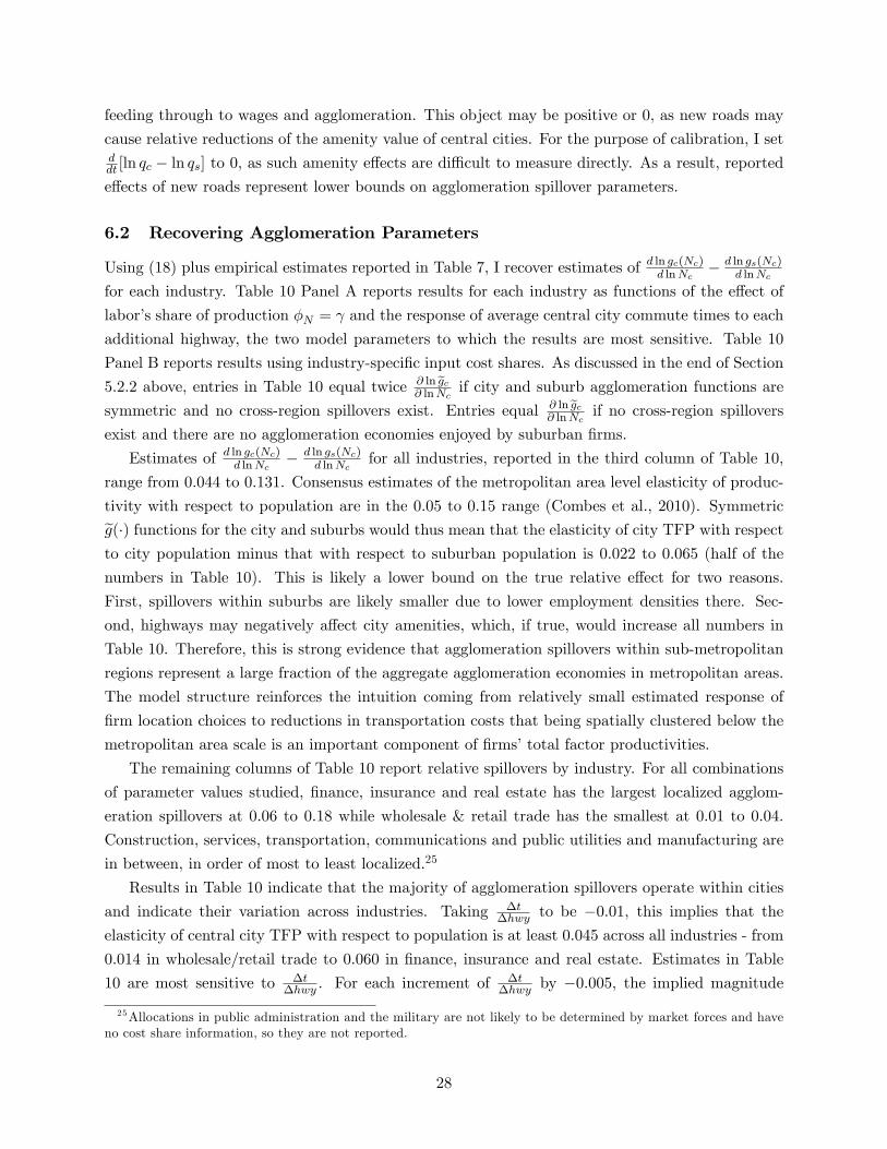
feeding through to wages and agglomeration. This object may be positive or 0, as new roads may
cause relative reductions of the amenity value of central cities. For the purpose of calibration, I setddt [ln qc � ln qs] to 0, as such amenity e¤ects are di¢ cult to measure directly. As a result, reportede¤ects of new roads represent lower bounds on agglomeration spillover parameters.
6.2 Recovering Agglomeration Parameters
Using (18) plus empirical estimates reported in Table 7, I recover estimates of d ln gc(Nc)d lnNc� d ln gs(Nc)
d lnNc
for each industry. Table 10 Panel A reports results for each industry as functions of the e¤ect of
labor�s share of production �N = and the response of average central city commute times to each
additional highway, the two model parameters to which the results are most sensitive. Table 10
Panel B reports results using industry-speci�c input cost shares. As discussed in the end of Section
5.2.2 above, entries in Table 10 equal twice @ ln egc@ lnNc
if city and suburb agglomeration functions are
symmetric and no cross-region spillovers exist. Entries equal @ ln egc@ lnNc
if no cross-region spillovers
exist and there are no agglomeration economies enjoyed by suburban �rms.
Estimates of d ln gc(Nc)d lnNc� d ln gs(Nc)
d lnNcfor all industries, reported in the third column of Table 10,
range from 0:044 to 0:131. Consensus estimates of the metropolitan area level elasticity of produc-
tivity with respect to population are in the 0:05 to 0:15 range (Combes et al., 2010). Symmetriceg(�) functions for the city and suburbs would thus mean that the elasticity of city TFP with respectto city population minus that with respect to suburban population is 0:022 to 0:065 (half of the
numbers in Table 10). This is likely a lower bound on the true relative e¤ect for two reasons.
First, spillovers within suburbs are likely smaller due to lower employment densities there. Sec-
ond, highways may negatively a¤ect city amenities, which, if true, would increase all numbers in
Table 10. Therefore, this is strong evidence that agglomeration spillovers within sub-metropolitan
regions represent a large fraction of the aggregate agglomeration economies in metropolitan areas.
The model structure reinforces the intuition coming from relatively small estimated response of
�rm location choices to reductions in transportation costs that being spatially clustered below the
metropolitan area scale is an important component of �rms�total factor productivities.
The remaining columns of Table 10 report relative spillovers by industry. For all combinations
of parameter values studied, �nance, insurance and real estate has the largest localized agglom-
eration spillovers at 0:06 to 0:18 while wholesale & retail trade has the smallest at 0:01 to 0:04.
Construction, services, transportation, communications and public utilities and manufacturing are
in between, in order of most to least localized.25
Results in Table 10 indicate that the majority of agglomeration spillovers operate within cities
and indicate their variation across industries. Taking �t�hwy to be �0:01, this implies that the
elasticity of central city TFP with respect to population is at least 0:045 across all industries - from
0:014 in wholesale/retail trade to 0:060 in �nance, insurance and real estate. Estimates in Table
10 are most sensitive to �t�hwy . For each increment of
�t�hwy by �0:005, the implied magnitude
25Allocations in public administration and the military are not likely to be determined by market forces and haveno cost share information, so they are not reported.
28

of localized agglomeration spillovers in a metropolitan area increases by 0.03-0.05 conditional on
all other parameter values examined. As additional highways cause commuting times to fall more
quickly (and �t�hwy rises in absolute value), we infer a smaller change in central city employment for
a given change in t. The model interprets this smaller change as evidence of stronger agglomeration
forces keeping �rms in the central city.
By making use of (21) jointly with (18), it is in principle possible to recover separate estimates
for d ln gcd lnNcand d ln gs
d lnNc. However, carrying out this exercise yields implied values for d ln gcd lnNc
that depend
very sensitively on �t�hwy . In particular, each reduction in
�t�hwy of 0:0025 results in an increase
of d ln gcd lnNc
by 0:44. Therefore, separating precise quanti�cation of d ln gcd lnNc
from d ln gsd lnNc
is impossible
using this framework. However, beyond its information on the relative magnitudes of agglomeration
spillovers, we can also use this framework to learn quantitatively about the mechanisms driving
urban decentralization and the welfare consequences of new highways.
6.3 Why Did Highways Cause Suburbanization?
Table 11 reports calibrated values for each component of � lnQc�hwy using (21), where � lnQc
�hwy �d lnQcdt
�t�hwy under di¤erent assumptions about the labor share , how highways a¤ect commute
times �t�hwy , and the income elasticity of demand for housing �. Results in columns A-H match
the same components of � lnQc�hwy enumerated in (21), with each element of (21) multiplied by�t
�hwy .
For columns A-H, I impose that d ln gcd lnNc
= 0 and d lnhdt = 0, assumptions that are relaxed in the
remaining columns of Table 11. Given a value for d lnNcdt , smaller working population responses to
new highways indicates more localized agglomeration spillovers for central city �rms. By imposingd ln gcd lnNc
= 0, each entry thus provides an upper bound on the true magnitude of each component. The
�rst column in the right block in Table 11 separately reports the additional contribution assumingd lnhdt = �1 through wage e¤ects in Components C,D and E plus �rm land use changes in I. The
�nal column of Table 11 reports the countervailing positive contribution of d ln gcd lnNc
, assuming thatd ln gcd lnNc
is one-half of the corresponding value forhd ln gcd lnNc
� d ln gsd lnNc
ireported in Table 10, meaning
central area and suburban agglomeration functions are symmetric and cross-region spillovers are
0. These are conservative estimates, as weaker suburban agglomeration spillovers would cause the
true value of d ln gcd lnNc
to be larger. In the extreme, if only within-city spillovers existed, the e¤ects
of relaxing d ln gcd lnNc
= 0 would be twice as large as those reported in the �nal column. Components
listed in Table 11 should be compared to the full treatment e¤ect of �0:16 of each highway oncentral area working population reported in Table 7.
Following are the most important mechanisms through which highways caused urban population
decentralization. Factor reallocation toward land in housing production (Component F) is the
largest negative component at between �0:033 and �0:098 depending on parameters, or up to 60percent of the full estimated treatment e¤ect. Firm adjustments to space per worker (Component
G) adds �0:021 to �0:064 to this, but is somewhat counterbalanced by the crowd-in e¤ect of �rmsmoving operations to the suburbs (Component H) of 0:029. Price & income e¤ect mechanisms and
factor reallocation in housing production because of wage changes sum to no more than �0:05,
29

mostly because of components A and B. These results indicate that key to understanding urban
decentralization is the high land share in the production of housing. People live on more space
as highways cause central area rents to decline, thereby generating lower densities and population
decentralization.
The �nal two columns of Table 11 show the additional impacts that operate through shifts in
�rm productivity. Imposing d lnhdt = �1 generates up to an additional �0:032 or 5-20 percent of the
full treatment e¤ect. As seen in the �nal column, imposing d ln gcd lnNc
as one-half ofhd ln gcd lnNc
� d ln gsd lnNc
iresults in small positive impacts of less than 0:01 to �lnQc
�hwy . If the maximum possible estimates ofd ln gcd lnNc
from Table 10 are used instead, e¤ects on population decentralization rise to less than 0:02.
6.4 Evaluating Welfare Consequences
In this sub-section, I evaluate the welfare consequences of new highways using the model. From
(12), residents�willingness to pay for a new highway (on the margin) is:
�Vc=�[hwy]
�c� [wc(1� t)] [
d lnwcdt
� 1]��t
�hwy
�� [pcH] [�L
d ln r
dt+ �N
d lnwcdt
]
��t
�hwy
�(21)
Analogous expressions for commutes involving the suburbs yield identical implications. The �rst
term captures the increase in real income that occurs both because the new highway increases
commuting speed and because it raises wages through the three mechanisms speci�ed in (20).
This increase in real income can be expressed as a fraction of initial central city income net of
commuting cost wc(1 � t). The second term captures the welfare consequences of changes in
housing cost, and can be expressed as a fraction of central city housing cost pcH. The change in
housing cost re�ects the change in land and labor costs given in (19) and (20) respectively, which
push in opposite directions. With su¢ ciently strong productivity gains from new highways, housing
costs can actually increase. Expressed in this way, welfare implications can be applied broadly to
cities of di¤erent income levels and housing costs, though putting them in dollar terms requires
knowledge of wage and house price levels.
While residents experience clear welfare gains from new highways, landowners experience clear
welfare losses because central space declines in value. The aggregate capital loss for absentee
landlords is rLc d ln rdt
h�t
�hwy
i. Of course, central city owner-occupiers will incur this capital loss
along with the other welfare gains.
Table 12 presents the welfare results. A central input into welfare calculations is how much
central city wages are a¤ected by reductions in transport costs. Such wage responses depend
crucially on assumptions about d lnhdt and d ln gc
d lnNc. As in Table 11, I determine the in�uences of
each of these components by presenting results with and without their inclusion and assuming thatd ln gcd lnNc
equals one-half ofhd ln gcd lnNc
� d ln gsd lnNc
ireported in Table 10. Columns 4-7 of Table 12 break
down how real income changes in percentage terms with each additional radial highway assuming
no productivity changes, productivity changes through changes in metro level agglomeration h(t)
only, productivity changes through changes in local spillovers gc(Nc) only, and those through both
30

together, respectively.
The reduction in commuting cost plus increase in the land/labor ratio associated with each
new highway raises real income by 0.6 to 2 percent, depending on parameter values (Column 4).
Addition of the direct e¤ect of transport costs on TFP, assuming that d lnhdt = �1, raises this
to up to 4.1 percent. However, incorporating local agglomeration spillovers instead lowers these
gains to no more than 1.4 percent. This is because such spillovers decline with the employment
decentralization that happens because of the new highways. Incorporating all three mechanisms
simultaneously yields estimated real income increases of 1.1 to 3.6 percent per highway. These
are upper bounds since d lnhdt is likely to be between 0 and 1 and d ln gc
d lnNcis larger if suburban
agglomeration spillovers are weaker.
Table 12 Columns 8-11 report impacts of one new radial highway on real housing cost in per-
centage terms. Because wages are only a small component of housing cost, housing cost e¤ects vary
less across parameter values and considered mechanisms, from a decline of 0.5 percent to a decline
of 3 percent, with the greatest declines occurring in environments in which wages rise the least.
Given that only 17 percent of income goes to housing services, the impacts of housing cost declines
on overall welfare are much smaller than the associated income gains. Central city rent declines of
4 to 13 percent with each new highway means that the associated total impact on housing costs
of each new highway for owner-occupiers is negligible relative to the associated impact on income.
Table 12 Column 12 shows the e¤ects of a new highway on central city rents. These declines range
from 8% to 13%.
Taken together, results in Table 12 indicate that each new highway generating a willingness to
pay of 1-4 percent of income for renters. The capital loss from reduced city land values reduces
this amount by less than one percentage point for owners.
7 Conclusions
This paper demonstrates that new radial highways have caused signi�cantly greater amounts of
residential than job decentralization. Each radial highway displaced an estimated 16 percent of the
central city working population but only 6 percent of the jobs to the suburbs. These estimates are
fairly consistent across industry, though are larger in absolute value for retail and wholesale trade
and smaller for �nance, insurance and real estate.
Viewed in the context of a calibrated urban model, these results provide evidence that local
spillovers are an important incentive for �rms to cluster spatially. Using estimated treatment e¤ects
and calibrated cost and expenditure shares, the implied elasticity of central city TFP to central
city employment relative to suburban employment is 0.02-0.05, meaning that a large fraction of
overall agglomeration economies operate at spatial scales below the metropolitan area level.
Model calibration results also bring forth reasons for the success of the monocentric model
for understanding urban population decentralization, despite its restrictive assumption that all
employment is located at the center. Results indicate that factor reallocation toward land in
31

housing and traded goods production generates the majority of population decentralization with
new highways, with only small additional e¤ects due to employment relocations.
Welfare analysis reveals that each radial highway causes central city income net of commuting
costs to increase by up to 3.6% and housing cost to decline by up to 3.0%. Therefore, each radial
highway increased metropolitan area output by 1 to 4 percent on the margin.
32
References
Ahlfeldt, Gabriel, Stephen Redding, Daniel Sturm and Niko Wolf (2015) "The Economics of
Density: Evidence from the Berlin Wall," Econometrica, 83(6): 2127-2189.
Albouy, David (2016) �What Are Cities Worth? Land Rents, Local Productivity, and the Total
Value of Amenities,�Review of Economics and Statistics, 98(3): 477-487.
Albouy, David and Bryan Stuart (2016) "Urban Population and Amenities: The Neoclassical
Model of Location," manuscript.
Allen, Treb & Costas Arkolakis (2014) "Trade and the Topography of the Spatial Economy,"
129(3), 1085-1140.
Allen, Treb, Costas Arkolakis & Xiangliang Li (2015) "Optimal City Structure," manuscript.
Alonso, William (1964) "Location and Land Use" (Cambridge: Harvard University Press).
Arzaghi, Mohammad & J. Vernon Henderson (2008) "Networking o¤Madison Avenue," Review
of Economic Studies, 75(4): 1011-1038.
Bartik, Timothy J. (1991) "Who Bene�ts from State and Local Economic Development Poli-
cies?" Upjohn Press. W.E. Upjohn Institute for Employment Research.
Baum-Snow, Nathaniel (2007a) "Did Highways Cause Suburbanization?" Quarterly Journal of
Economics 122(2): 775-805.
Baum-Snow, Nathaniel (2007b) "Suburbanization and Transportation in the Monocentric Model"
Journal of Urban Economics, 62(3): 405-423.
Baum-Snow, Nathaniel (2010) "Changes in Transportation Infrastructure and Commuting Pat-
terns in U.S. Metropolitan Areas, 1960-2000," American Economic Review Papers & Proceedings,
100(2): 378-382.
Baum-Snow, Nathaniel, Loren Brandt, J. Vernon Henderson, Matthew A. Turner and Qinghua
Zhang (2016) "Roads, Railways and Decentralization of Chinese Cities," Review of Economics and
Statistics, forthcoming.
Baum-Snow, Nathaniel and Byron Lutz (2011) "School Desegregation, School Choice and
Changes in Residential Location Patterns by Race," American Economic Review, 101(7): 3019-
3046.
Billings, Stephen and Erik Johnson (2016) "Agglomeration within an urban area," Journal of
Urban Economics 91:13-25.
Brinkman, Je¤rey (2016) "Congestion, Agglomeration, and the Structure of Cities," Journal of
Urban Economics, 94, 13-31.
Brinkman, Je¤rey, Daniele Coen-Pirani and Holger Sieg (2015) "Firm Dynamics in an Urban
Economy," International Economic Review, 56:4, 1135�1164.
Carliner, Michael (2003) �New Home Cost Components.�Housing Economics, 51: 7-11.
Combes, Pierre-Philippe, Gilles Duranton, Laurent Gobillon and Sébastien Roux (2010) "Esti-
mating Agglomeration Economies with History, Geology, and Worker E¤ects." In Agglomeration
Economics, Edward L. Glaeser (ed.), NBER, Cambridge, MA.
33

Combes, Pierre-Philippe & Laurent Gobillon (2015) "Empirics of Agglomeration Economies,"
in Handbook of Urban and Regional Economics Vol. 5, Duranton, Gilles, Henderson, J.Vernon &
William Strange eds., Elsevier, Amsterdam.
Couture, Victor, Gilles Duranton & Matthew A. Turner (2016) "Speed," Review of Economics
and Statistics, forthcoming.
Couture, Victor & Jessie Handbury (2016) "Urban Revival in America," manuscript.
Davis, Morris and François Ortalo-Magné (2011) "Household Expenditures, Wages, Rents"
Review of Economic Dynamics 14(2), 248-261.
Davis, Morris and Michael Palumbo (2007) �The Price of Residential Land in Large U.S. Cities.�
Journal of Urban Economics 63, 352-384.
Duranton, Gilles & Henry Overman (2005) "Testing for Localization Using Microgeographic
Data," Review of Economic Studies, 72 (4): 1077-1106.
Duranton, Gilles, Peter Morrow & Matthew A. Turner (2014) "Roads and Trade: Evidence
from the U.S." Review of Economic Studies, 81(2), 681-724.
Duranton, Gilles & Matthew A. Turner (2012) "Urban Growth and Transportation," Review
of Economic Studies, 79(4): 1407-1440.
Ellison, Glenn & Edward Glaeser (1997) "Geographic concentration in US manufacturing in-
dustries: a dartboard approach," Journal of Political Economy, 105(5): 889-927.
Ellison, Glenn, Edward Glaeser & William Kerr (2010) "What causes industry agglomeration?
Evidence from coagglomeration patterns," American Economic Review, 100(3): 1195-1213.
Fu, Shihe and Stephen L. Ross. (2013) "Wage Premia in Employment Clusters: How Important
is Worker Heterogeneity?" Journal of Labor Economics 31:2, 271-304.
Fujita, Masahisa & H. Ogawa (1982) "Multiple Equilibria and Structural Transition of Non-
monocentric Urban Con�gurations," Regional Science and Urban Economics 12(1): 161-196.
Fujita, Masahisa (1989) "Urban Economic Theory: Land Use and City Size" (Cambridge:
Cambridge University Press)
Glaeser, Edward & Joseph Gyourko (2005) "Urban Decline and Durable Housing" Journal of
Political Economy, 113(2): 345-375.
Glaeser, Edward & Matthew E. Kahn (2001) "Decentralized Employment and the Transforma-
tion of the American City" Brookings-Wharton Papers on Urban A¤airs 2: 1-63.
Glaeser, Edward, Matthew Kahn & Jordan Rappaport (2008) "Why Do the Poor Live in Cities?
The Role of Public Transportation" Journal of Urban Economics 63(1), 1-24.
Glaeser, Edward, Jed Kolko & Albert Saiz (2001) "Consumer City" Journal of Economic Ge-
ography 1(1), 27-50.
Greenstone, Michael, Richard Hornbeck & Enrico Moretti (2010) "Identifying agglomeration
spillovers: Evidence from winners and losers of large plant openings," Journal of Political Economy,
118(3): 536-598.
Helsley, Robert W. and William C. Strange (2014) �Coagglomeration and the Scale and Com-
position of Clusters,�Journal of Political Economy, 122(5): 1064-1093.
34

Lucas, Robert E. & Esteban Rossi-Hansberg (2002) "On the Internal Structure of Cities,"
Econometrica 70(4): 1445-1476.
Mayo, Stephen (1981) "Theory and Estimation in the Economics of Housing Demand," Journal
of Urban Economics 10: 95-116.
Michaels, Guy (2008) "The E¤ect of Trade on the Demand for Skill - Evidence from the Inter-
state Highway System," Review of Economics and Statistics, 90(4): 683-701.
Mills, Edwin S. (1967) �An Aggregative Model of Resource Allocation in a Metropolitan Area,�
American Economic Review, LVII: 197-210.
Muth, Richard F. (1969) "Cities and Housing" (Chicago: University of Chicago Press).
Ogawa, H. & Masahisa Fujita (1980) "Equilibrium Land Use Patterns in a Non-monocentric
City," Journal of Regional Science 20: 455-475.
Rossi-Hansberg, Esteban, Pierre-Daniel Sarte and Raymond Owens III (2009) "Firm Fragmen-
tation and Urban Patterns," International Economic Review 50(1): 143-186.
Rand McNally Co. (1960) Leahy�s Hotel-Motel Guide and Travel Atlas of the United States,
Canada and Mexico, American Hotel Register Company. Chicago, IL.
Rand McNally Co. (2000) Rand McNally Road Atlas: United States, Canada, Mexico. Rand
McNally Co., New York, NY
Rosen, Sherwin (1979) �Wage-Based Indexes of Urban Quality of Life,� in Peter Mieszkowski
and Mahlon Straszheim eds. Current Issues in Urban Economics, Baltimore: Johns Hopkins Uni-
versity Press.
Rosenthal, Stuart & William Strange (2003) "Geography, Industrial Organization, and Agglom-
eration," Review of Economics and Statistics, 85(2): 377-393.
Roback, Jennifer (1982) �Wages, Rents and the Quality of Life,�Journal of Political Economy
90: 1257-1278.
Saiz, Albert (2010) "The Geographic Determinants of Housing Supply," Quarterly Journal of
Economics 125 (3): 1253-1296.
U.S. Department of Transportation (1977) America�s Highways: 1776-1976: A History of the
Federal-Aid Program, U.S. Government Printing O¢ ce, Washington.
35

Figure 1: Davenport SMSA
SMSA Boundary
Davenport
Rock Island
Moline
2000 Traffic Analysis Zone Boundary
1960 City Boundary
2000 City Boundary

Figure 2: CDFs and Changes in Working Residential Population by Residential Location1960-2000 (0=CBD, 1=Central City Edge)
Panel A: All Locations Pooled
Panel B: Primary Central City and Suburban Residents Broken Out
Notes: Plots show cumulative distribution functions of SMSA residents in 1960 and 2000. The distance index onthe horizontal axis is 0 at the CBD and 1 at the furthest location on the edge of the primary central city. Suburbantracts with index values of less than 1 are closer to the CBD than the furthest central city location. 78 of the 100SMSAs with at least 250,000 residents in 1960 contribute to the plots. The remaining 22 are not included becauseof missing or incomplete 1960 census tract information.
-0.5
0.5
1.5
2.5
-0.5
0
0.5
1
0 0.5 1 1.5 2 2.5 3
CC, 2000
CC , 1960 Suburban, 1960Suburban, 2000
Dln(Pop) Suburban(right axis)
Dln(Pop) CC(right axis)
-0.5
0.5
1.5
2.5
-0.5
0
0.5
1
0 0.5 1 1.5 2 2.5 3
1960 CDF
2000 CDF
Dln(Pop)(right axis)

Figure 3: Average Fraction Commuting to Primary Central Cityby Residential Location (0=CBD, 1=Central City Edge)
Notes: Plots show the fraction of workers in 1960 and 2000 commuting to a primary central city averaged acrossSMSAs The distance index on the horizontal axis is 0 at the CBD and 1 at the furthest location on the central cityedge.
Panel A: All Locations Pooled
Panel B: Central City and Suburban Residents Broken Out
0
0.25
0.5
0.75
1
0 0.5 1 1.5 2 2.5 3
Central City Residents, 2000
Suburban Residents, 1960
Suburban Residents, 2000
Central City Residents, 1960
0
0.25
0.5
0.75
1
0 0.5 1 1.5 2 2.5 3
1960
2000
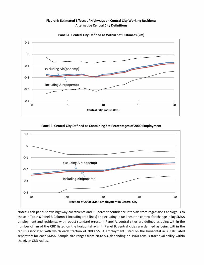
Figure 4: Estimated Effects of Highways on Central City Working ResidentsAlternative Central City Definitions
Panel A: Central City Defined as Within Set Distances (km)
Panel B: Central City Defined as Containing Set Percentages of 2000 Employment
Notes: Each panel shows highway coefficients and 95 percent confidence intervals from regressions analogous tothose in Table 6 Panel B Column 1 including (red lines) and exluding (blue lines) the control for change in log SMSAemployment and residents, with robust standard errors. In Panel A, central cities are defined as being within thenumber of km of the CBD listed on the horizontal axis. In Panel B, central cities are defined as being within theradius associated with which each fraction of 2000 SMSA employment listed on the horizontal axis, calculatedseparately for each SMSA. Sample size ranges from 78 to 93, depending on 1960 census tract availability withinthe given CBD radius.
-0.4
-0.3
-0.2
-0.1
0
0.1
0 5 10 15 20Central City Radius (km)
-0.4
-0.3
-0.2
-0.1
0
0.1
10 20 30 40 50Fraction of 2000 SMSA Employment in Central City
including Dln(popemp)
excluding Dln(popemp)
including Dln(popemp)
excluding Dln(popemp)

1960 2000 Percent Change Change in FractionLive in Central City 18.7 18.4 -0.01 -0.25 (fraction of total) (0.49) (0.24)Work in Central City 23.3 26.2 0.12 -0.28 (fraction of total) (0.61) (0.34)Live in SMSA 36.3 66.8 0.84 -0.10 (fraction of total) (0.95) (0.86)Work in SMSA 36.8 71.1 0.93 -0.05 (fraction of total) (0.96) (0.91)
Live or Work in SMSA 38.1 78.1 1.05
Notes: Counts are aggregates from the 100 metropolitan areas with 1960 populations over 250,000,expressed in millions of workers. Counts are calculated using 1960 and 2000 census journey to work datausing 1960 SMSA definitions. Those contributing to residential counts may work anywhere and thosecontributing to worker counts may live anywhere. Data from 1960 incorporate the author's imputations fornonreported work locations. Data from 2000 incorporate such imputations done by the Census Bureau andthe author.
Table 1: Changes in Residential and Work Locations, 1960-2000100 Metropolitan Areas With 1960 Populations Over 250,000

All Manuf- Services Trade TCPU Const- Public FIRE Military Agric-acturing ruction Admin. ulture
Live in Central City1 1960 Fraction in CC 0.52 0.49 0.56 0.54 0.55 0.45 0.56 0.57 0.39 0.202 1960-2000 Change in CC Fraction -0.24 -0.25 -0.25 -0.30 -0.26 -0.20 -0.28 -0.30 -0.18 -0.04Work in Central City3 1960 Fraction in CC 0.63 0.60 0.64 0.67 0.73 0.56 0.68 0.79 0.40 0.214 1960-2000 Change in CC Fraction -0.27 -0.33 -0.24 -0.39 -0.32 -0.24 -0.16 -0.37 -0.09 0.00Live in Entire SMSA5 1960 Fraction of All 1.00 0.30 0.22 0.19 0.08 0.06 0.06 0.05 0.02 0.026 1960-2000 Change in Fraction of All 0.00 -0.17 0.21 -0.04 0.01 0.00 -0.01 0.03 -0.01 -0.01Work in Entire SMSA7 1960 Fraction of All 1.00 0.30 0.22 0.19 0.08 0.06 0.06 0.05 0.02 0.028 1960-2000 Change in Fraction of All 0.00 -0.18 0.21 -0.04 0.01 0.01 -0.01 0.03 -0.01 -0.01
Table 2: Changes in Residential and Work Locations by Industry, 1960-2000
Notes: Counts used to construct entries are aggregated over all primary sample SMSAs. See the notes to Table 1 for an explanation of the sample and data sources. Because the 2000 CensusTransportation Planning Package does not report commuting flows by industry, changes in counts of people by industry who either live or work in SMSAs are not available.

1960 2000 Change Weighted UnweightedLive in CC Work in CC 16.5 12.0 -27% 27 19
(0.43) (0.16) -0.28 1 1Live in CC Work in Ring 1.8 5.0 177% 30 26
(0.05) (0.06) 0.02 1.13 1.38Live in CC Work Outside SMSA 0.4 1.0 127% 46 46
(0.01) (0.01) 0.00 1.73 2.46Live in Ring Work in CC 5.9 10.7 82% 33 27
(0.15) (0.14) -0.01 1.25 1.46Live in Ring Work in Ring 10.8 32.4 200% 22 20
(0.28) (0.42) 0.14 0.85 1.07Live in Ring Work Outside SMSA 0.9 4.4 384% 41 40
(0.02) (0.06) 0.03 1.53 2.14Live Outside SMSA Work in CC 1.0 3.9 294% 54 47
(0.03) (0.05) 0.02 2.02 2.52Live Outside SMSA Work in Ring 0.9 7.4 735% 43 41
(0.02) (0.10) 0.07 1.63 2.19
Total 38.1 76.7 101%
Avg. 2000 Commute Time
Table 3: Changes in Commuting Patterns, 1960-2000
Notes: Each entry in the first two columns is the number of people with the indicated type of commute in the indicated year in millions.The fraction of total commutes in the indicated year is in parentheses. The 2000 total does not exactly match the total in Table 1 becausethe Census Bureau omits some difficult to impute flows in its Census Transportation Planning Package tables. Those working at home arecounted as commuting within their regions of residence. Column 4 shows one-way commute times averaged across all workers in sampledSMSAs and ratios relative to the average within central city commute time. Column 5 shows mean SMSA one-way commute timesaveraged across sampled SMSAs and ratios relative to this measure of within central city commute time. Commuting times are notavailable for 1960.

(1) (2) (3)Planned Rays 0.53*** 0.47*** 0.47***
(0.12) (0.12) (0.11)1960 Central City Radius 0.11 0.10
(0.10) (0.09)Change in Log SMSA Employment 0.32 +Workers, 1960-2000 (0.44)Constant 1.13*** 0.80* 0.62
(0.33) (0.44) (0.52)Adj. R-Squared 0.23 0.24 0.25
Planned Rays 0.36*** 0.34*** 0.33***(0.11) (0.11) (0.11)
1960 Central City Radius 0.04 0.03(0.09) (0.09)
Change in Log SMSA Employment 0.29 +Workers, 1960-2000 (0.41)Constant 0.94*** 0.81* 0.65
(0.31) (0.43) (0.53)Adj. R-Squared 0.11 0.12 0.12
Panel A: 1950 Base Year
Panel B: 1960 Base Year
Table 4: First Stage Results
Notes: Regression results are of changes in actual radial highways constructed between1950 and 2000 (Panel A) or 1960 and 2000 (Panel B) on the listed variables for the 100SMSAs in the primary sample. Robust standard errors are in parentheses. Regressionsusing the number of radial highways in 2000 instead are statistically indistinguishiblefrom those in Panel A. Additional inclusion of log 1950 SMSA population, 1940-1950SMSA population growth and 1 digit SMSA employment shares from 1940 do notstatistically influence planned rays coefficient estimates. Coefficients on planned rays inanalogous regressions using a more complete sample of 164 SMSAs are statisticallysignificant at 0.42 and 0.28 in Columns 2 or 3 of Panels A and B respectively.

All Manuf- Services Trade TCPU Const- Public FIRE Military Agric-acturing ruction Admin. ulture
Change in Rays 0.03 -0.11*** -0.00 -0.01 0.01 0.03 -0.06 0.04 0.05 -0.01 1950 to 2000 (0.05) (0.04) (0.01) (0.01) (0.03) (0.03) (0.04) (0.03) (0.13) (0.06)1960 Central City Radius 0.04* 0.05** 0.00 -0.01 -0.00 0.01 -0.02 -0.03** -0.11** 0.03
(0.02) (0.02) (0.01) (0.01) (0.01) (0.01) (0.02) (0.01) (0.06) (0.03)Change in Log SMSA Employment 1.40*** 0.82*** 0.94*** 1.15*** 0.80*** 0.83*** 0.89*** 0.51 0.39*** +Workers, 1960-2000 (0.09) (0.03) (0.02) (0.05) (0.05) (0.07) (0.05) (0.35) (0.13)Constant 0.43*** -1.03*** 0.74*** -0.18*** -0.07 0.01 0.21** 0.52*** -0.41 -1.18***
(0.13) (0.09) (0.03) (0.04) (0.08) (0.07) (0.11) (0.07) (0.29) (0.17)Adj. R-Squared 0.07 0.75 0.91 0.93 0.84 0.80 0.54 0.77 0.06 0.17
Change in Rays -0.00 -0.14*** -0.03 -0.05*** -0.02 -0.01 -0.09* -0.00 -0.04 -0.05 1950 to 2000 (0.05) (0.04) (0.02) (0.02) (0.03) (0.03) (0.05) (0.03) (0.12) (0.06)1960 Central City Radius 0.05* 0.05** 0.01 -0.00 0.00 0.01 -0.01 -0.02* -0.08 0.03
(0.02) (0.02) (0.01) (0.01) (0.01) (0.01) (0.02) (0.01) (0.06) (0.03)Change in Log SMSA Employment 1.38*** 0.81*** 0.94*** 1.12*** 0.80*** 0.81*** 0.90*** 0.52 0.43*** +Workers, 1960-2000 (0.10) (0.04) (0.03) (0.05) (0.06) (0.07) (0.05) (0.36) (0.13)Constant 0.44*** -0.99*** 0.74*** -0.17*** -0.07 0.01 0.21* 0.52*** -0.40 -1.18***
(0.13) (0.10) (0.04) (0.04) (0.07) (0.08) (0.11) (0.06) (0.27) (0.17)Adj. R-Squared 0.05 0.71 0.85 0.87 0.83 0.75 0.51 0.78 0.07 0.12
Panel B: SMSA Working Residents
Panel A: SMSA Employment
Table 5: Effects of Highways on SMSA Employment and Working Residents by IndustryIV Estimates
Notes: Regressions are of the change in the log of outcomes listed in column headers on variables listed at left. These are Equations (3) and (4) in the text. The sample includesthe same 100 SMSAs used for Tables 1 through 4. The change in the number of rays is instrumented with rays in the 1947 national plan. Robust standard errors are inparentheses. The estimated effect of highways on total SMSA employment plus resident workers is identical to that for all employment in Panel A. Excluding the change in logSMSA employment+workers yields no significant change in any highways coefficient. The first-stage F statistic for all industry level regressions is 16.75.

All Manuf- Services Trade TCPU Const- Public FIRE Military Agric-acturing ruction Admin. ulture
Change in Rays -0.06* -0.16*** -0.07** -0.15*** -0.06 -0.05 -0.04 -0.02 0.07 0.15 1950 to 2000 (0.03) (0.06) (0.03) (0.06) (0.05) (0.04) (0.04) (0.06) (0.17) (0.10)1960 Central City Radius 0.05*** 0.11*** 0.05*** 0.10*** 0.07*** 0.06*** -0.04** 0.05** -0.11 -0.01
(0.01) (0.04) (0.02) (0.03) (0.02) (0.02) (0.02) (0.02) (0.07) (0.04)Change in Log Total 0.81*** 1.01*** 0.58*** 0.77*** 0.87*** 0.58*** 0.78*** 0.59*** 0.48 0.37** Employment+Residents (0.07) (0.12) (0.06) (0.10) (0.06) (0.08) (0.08) (0.09) (0.34) (0.15)Constant -0.56*** -1.71*** 0.37*** -1.14*** -0.58*** -0.43*** 0.06 -0.20 -0.70* -1.44***
(0.08) (0.16) (0.07) (0.13) (0.09) (0.10) (0.10) (0.14) (0.39) (0.28)Adj. R-Squared 0.66 0.43 0.50 0.44 0.63 0.46 0.50 0.36 0.04 0.13
Change in Rays -0.16*** -0.26*** -0.16*** -0.21*** -0.14** -0.22*** -0.16*** -0.12** -0.13 -0.07 1950 to 2000 (0.05) (0.07) (0.05) (0.06) (0.06) (0.07) (0.06) (0.05) (0.16) (0.08)1960 Central City Radius 0.09*** 0.11*** 0.09*** 0.08*** 0.09*** 0.11*** 0.05* 0.07*** -0.00 -0.04
(0.02) (0.03) (0.02) (0.03) (0.02) (0.03) (0.03) (0.02) (0.08) (0.03)Change in Log Total 0.62*** 1.02*** 0.41*** 0.52*** 0.65*** 0.61*** 0.27*** 0.42*** -0.50 0.14 Employment+Residents (0.09) (0.16) (0.09) (0.12) (0.10) (0.13) (0.10) (0.08) (0.44) (0.15)Constant -0.51*** -1.50*** 0.30*** -0.65*** -0.57*** -0.45*** -0.29** -0.12 -0.46 -0.66**
(0.11) (0.19) (0.12) (0.14) (0.13) (0.17) (0.14) (0.11) (0.35) (0.26)Adj. R-Squared 0.32 0.22 0.06 -0.04 0.32 0.04 -0.04 0.21 0.01 -0.02
Notes: Regressions are of the change in the log of outcomes listed in column headers on variables listed at left. These are Equations (5) and (6) in the text. The sampleincludes the same 100 SMSAs used for Tables 1 through 4. The change in the number of rays is instrumented with rays in the 1947 national plan. Robust standard errorsare in parentheses. Excluding the change in log SMSA employment+residents yields no significant change in any highways coefficient. The first stage F statistics for allregressions is 16.75. Each regression has 100 observations except that for the military in Panel A, which is missing Canton, OH because it had 0 reported central citymilitary jobs in 2000.
Table 6: Effects of Highways on Central City Employment and Working Residents by IndustryIV Estimates
Panel B: Central City Working Residents
Panel A: Central City Employment

Employment Working Residents Difference
All -0.06* -0.16*** 0.10**(0.03) (0.06) (0.04)
All (Excluding control for -0.04 -0.14** 0.10** Dln popempSMSA) (0.06) (0.06) (0.04)Manufacturing -0.08 -0.15*** 0.07
(0.05) (0.05) (0.06)Services -0.07** -0.15*** 0.08**
(0.03) (0.05) (0.03)Retail and Wholesale Trade -0.14** -0.19*** 0.05
(0.05) (0.05) (0.04)TCPU -0.07* -0.13*** 0.06
(0.04) (0.05) (0.05)Construction -0.08** -0.21*** 0.14***
(0.04) (0.06) (0.05)Public Administration 0.01 -0.13*** 0.14**
(0.03) (0.05) (0.06)FIRE -0.04 -0.12*** 0.07
(0.05) (0.05) (0.05)Military 0.01 -0.14 0.16
(0.15) (0.27) (0.33)Agriculture 0.16** -0.05 0.21**
(0.07) (0.07) (0.09)
Table 7: Implied Effects of Each Highway on Urban Decentralizationby Industry
Notes: Entries give estimated effects of one radial highway on the log of central city employment orworking residents in the indicated industry holding the composition of SMSA industries constant.Equations (3), (4), (5) and (6) in the text plus a first stage equation that are jointly estimated by three-stage least squares are used along with (7) and (8) to generate reported coefficients and standard errorsclustered by SMSA. GMM point estimates are identical.

Work in Work in Work OutsideCentral City Ring SMSA
Change in Rays -0.16*** -0.03 -0.03 1950 to 2000 (0.05) (0.06) (0.07)1960 Central City Radius 0.14*** 0.07** 0.07***
(0.02) (0.03) (0.02)Change in Log Total 0.50*** 0.77*** 0.07 Employment+Residents (0.10) (0.10) (0.14)Constant -1.11*** 0.22 0.66***
(0.12) (0.14) (0.17)
Change in Rays -0.06 0.11** 0.07 1950 to 2000 (0.08) (0.05) (0.08)1960 Central City Radius 0.10** 0.02 0.05
(0.04) (0.02) (0.03)Change in Log Total 1.08*** 1.25*** 0.84*** Employment+Residents (0.16) (0.09) (0.12)Constant -0.36** -0.14 0.95***
(0.18) (0.12) (0.16)
Change in Rays -0.09 0.22** 1950 to 2000 (0.06) (0.08)1960 Central City Radius 0.13*** 0.02
(0.02) (0.03)Change in Log Total 0.88*** 1.32*** Employment+Residents (0.11) (0.14)Constant 0.36** 0.52**
(0.14) (0.21)
Table 8: Estimated Effects of Highways on Aggregate Commuting Flows
Panel A: Central City Residents
Panel B: Suburban Residents
Panel C: Residents Outside SMSA Who Work in SMSA
Notes: Each column in each panel shows regression results of the change in the log number ofindicated commuters between 1960 and 2000 on variables listed at left. Radial highways inthe 1947 national plan instruments for the change in the number of rays 1950 to 2000. Robuststandard errors are in parentheses. The first-stage F-statistic for each regression is 16.75.

Parameter Description Man. Services Trade TCPU Cons. FIRE Agric.Dt/Dhwy Change in central city commuting time for each additional highway -0.01
h Income elasticity of demand for housing 0.7e Price elasticity of demand for housing -1sH Share of income spent on housing 0.17
qL Land share in production of housing 0.233
qK Capital Share in the production of housing 0.15
qN Labor share in the production of housing 0.617
fL Land share in production of tradeables 0.025 0.024 0.005 0.015 0.015 0.007 0.038 0.161
fK, m Capital Share in the production of tradeables 0.15 0.349 0.223 0.244 0.428 0.165 0.555 0.354
fN, g Labor share in the production of tradeables 0.825 0.627 0.772 0.741 0.556 0.828 0.407 0.485
Xc/(Lc-Xc) Fraction of CC space taken up by production 0.48t Fraction of time spent commuting for within central city commuters 0.06
csc Ratio of commuting time suburb-city versus city-city 1.75
cs Ratio of commuting time suburb-suburb versus city-city 1.36dlnh/dt The direct elasticity of TFP with respect to commuting time -1
Notes: Parameters' base calibration values are based on estimates in the literature, as explained in the text. Commuting cost parameters are calibrated using 2000 commuting data for primarysample SMSAs. Industry cost shares are taken from the KLEMS data.
Table 9: Base Parameter Values

fN, g Dt/Dhwy All Manufacturing Services Trade TCPU Construction FIRE Agriculture
0.6 -0.01 0.073 0.055 0.063 0.031 0.063 0.055 0.110 -0.0270.65 -0.01 0.076 0.057 0.065 0.033 0.065 0.057 0.114 -0.0290.7 -0.01 0.079 0.060 0.068 0.034 0.068 0.060 0.119 -0.030
0.75 -0.01 0.083 0.062 0.071 0.035 0.071 0.062 0.124 -0.0310.8 -0.01 0.086 0.064 0.073 0.037 0.073 0.064 0.129 -0.032
0.85 -0.01 0.089 0.067 0.076 0.038 0.076 0.067 0.133 -0.0330.825 -0.005 0.044 0.033 0.037 0.019 0.037 0.033 0.065 -0.0160.825 -0.01 0.087 0.065 0.075 0.037 0.075 0.065 0.131 -0.0330.825 -0.015 0.131 0.098 0.112 0.056 0.112 0.098 0.196 -0.049
0.7 -0.005 0.040 0.030 0.034 0.017 0.034 0.030 0.060 -0.0150.7 -0.01 0.079 0.060 0.068 0.034 0.068 0.060 0.119 -0.0300.7 -0.015 0.119 0.089 0.102 0.051 0.102 0.089 0.179 -0.045
-0.005 0.044 0.028 0.024 0.015 0.024 0.023 0.060 -0.049-0.0075 0.065 0.041 0.036 0.022 0.036 0.035 0.089 -0.073
-0.01 0.087 0.055 0.048 0.029 0.048 0.046 0.119 -0.097-0.0125 0.109 0.069 0.060 0.036 0.060 0.058 0.149 -0.121-0.015 0.131 0.083 0.071 0.044 0.072 0.070 0.179 -0.146
Notes: Entries quantify the aggregate own versus cross region agglomeration spillovers in a metropolitan area, as is described in the text,for each listed industry and combination of parameter values. Results in Panel A use common cost share parameters across columns. Resultsin Panel B use industry-specific cost shares taken from KLEMs data for the U.S. Additional calibrated parameter values are in Table 9.
Table 10: Agglomeration Parameters by Industry
Parameters dlngc/dlnNc - dlngs/dlnNc
Panel A: Common Cost Share Parameters
Panel B: Industry-Specific Cost Share Parameters

Additional AdditionalFrom From
fN, g Dt/Dhwy h A B C D E F G H dlnh/dt=-1 dlngc/dlnNc
0.6 -0.01 0.7 -0.007 -0.020 -0.002 0.002 -0.002 -0.065 -0.043 0.029 -0.020 0.004 -0.1230.65 -0.01 0.7 -0.007 -0.020 -0.002 0.002 -0.002 -0.065 -0.043 0.029 -0.018 0.004 -0.1140.7 -0.01 0.7 -0.007 -0.020 -0.002 0.002 -0.002 -0.065 -0.043 0.029 -0.017 0.004 -0.1060.75 -0.01 0.7 -0.007 -0.020 -0.002 0.002 -0.002 -0.065 -0.043 0.029 -0.016 0.004 -0.0990.8 -0.01 0.7 -0.007 -0.020 -0.002 0.002 -0.002 -0.065 -0.042 0.029 -0.015 0.004 -0.0920.85 -0.01 0.7 -0.007 -0.020 -0.002 0.002 -0.002 -0.065 -0.042 0.029 -0.014 0.004 -0.0870.825 -0.005 0.7 -0.004 -0.010 -0.001 0.001 -0.001 -0.033 -0.021 0.029 -0.007 0.002 -0.0450.825 -0.01 0.7 -0.007 -0.020 -0.002 0.002 -0.002 -0.065 -0.042 0.029 -0.014 0.004 -0.0900.825 -0.015 0.7 -0.011 -0.030 -0.003 0.002 -0.002 -0.098 -0.064 0.029 -0.022 0.006 -0.1350.7 -0.005 0.7 -0.004 -0.010 -0.001 0.001 -0.001 -0.033 -0.021 0.029 -0.008 0.002 -0.0530.7 -0.01 0.7 -0.007 -0.020 -0.002 0.002 -0.002 -0.065 -0.043 0.029 -0.017 0.004 -0.1060.7 -0.015 0.7 -0.011 -0.030 -0.003 0.003 -0.003 -0.098 -0.064 0.029 -0.025 0.006 -0.1590.6 -0.01 1 -0.010 -0.020 -0.004 0.002 -0.002 -0.065 -0.043 0.029 -0.025 0.005 -0.1550.65 -0.01 1 -0.010 -0.020 -0.003 0.002 -0.002 -0.065 -0.043 0.029 -0.023 0.005 -0.1430.7 -0.01 1 -0.010 -0.020 -0.003 0.002 -0.002 -0.065 -0.043 0.029 -0.021 0.005 -0.1320.75 -0.01 1 -0.010 -0.020 -0.003 0.002 -0.002 -0.065 -0.043 0.029 -0.020 0.005 -0.1240.8 -0.01 1 -0.010 -0.020 -0.003 0.002 -0.002 -0.065 -0.042 0.029 -0.019 0.005 -0.1160.85 -0.01 1 -0.010 -0.020 -0.003 0.002 -0.002 -0.065 -0.042 0.029 -0.017 0.005 -0.1090.825 -0.005 1 -0.005 -0.010 -0.001 0.001 -0.001 -0.033 -0.021 0.029 -0.009 0.002 -0.0560.825 -0.01 1 -0.010 -0.020 -0.003 0.002 -0.002 -0.065 -0.042 0.029 -0.018 0.005 -0.1120.825 -0.015 1 -0.015 -0.030 -0.004 0.002 -0.002 -0.098 -0.064 0.029 -0.027 0.007 -0.1690.7 -0.005 1 -0.005 -0.010 -0.002 0.001 -0.001 -0.033 -0.021 0.029 -0.011 0.003 -0.0660.7 -0.01 1 -0.010 -0.020 -0.003 0.002 -0.002 -0.065 -0.043 0.029 -0.021 0.005 -0.1320.7 -0.015 1 -0.015 -0.030 -0.005 0.003 -0.003 -0.098 -0.064 0.029 -0.032 0.008 -0.199
Notes: Entries give components of the estimated treatment effect of each radial highway on the log of central city resident workers of -0.16. Each component Athrough H is mathematically specified in (21) and explained in the text. Contributions from component I are incorporated in the final columns of the table. Entries inthe final column assume that dlngc/dlnNc is one-half of the numbers reported in the "All" column of Table 10.
Table 11: Mechanisms Through Which Highways Cause Suburbanization
Components of dlnQc/dhwy if dlngc/dNc=0 & dlnh/dt=0Parameters Price & Income Effects Housing Factor Realloc. Firm GE Effects

CC rent incr.fN, g Dt/Dhwy h (4) (5) (6) (7) (8) (9) (10) (11) (12)0.6 -0.01 0.7 1.4% 3.0% 1.0% 2.7% -1.8% -0.7% -2.0% -1.0% -8.5%
0.65 -0.01 0.7 1.3% 2.9% 1.0% 2.5% -1.8% -0.8% -2.0% -1.1% -8.5%0.7 -0.01 0.7 1.3% 2.7% 1.0% 2.4% -1.8% -0.9% -2.0% -1.1% -8.5%
0.75 -0.01 0.7 1.3% 2.6% 1.0% 2.3% -1.8% -1.0% -2.0% -1.2% -8.5%0.8 -0.01 0.7 1.3% 2.5% 0.9% 2.2% -1.8% -1.0% -2.0% -1.2% -8.5%
0.85 -0.01 0.7 1.3% 2.4% 0.9% 2.1% -1.8% -1.1% -2.0% -1.3% -8.5%0.825 -0.005 0.7 0.6% 1.2% 0.5% 1.1% -0.9% -0.5% -1.0% -0.6% -4.3%0.825 -0.01 0.7 1.3% 2.5% 0.9% 2.2% -1.8% -1.1% -2.0% -1.3% -8.5%0.825 -0.015 0.7 1.9% 3.7% 1.4% 3.2% -2.7% -1.6% -3.0% -1.9% -12.8%
0.7 -0.005 0.7 0.7% 1.4% 0.5% 1.2% -0.9% -0.5% -1.0% -0.6% -4.3%0.7 -0.01 0.7 1.3% 2.7% 1.0% 2.4% -1.8% -0.9% -2.0% -1.1% -8.5%0.7 -0.015 0.7 2.0% 4.1% 1.4% 3.6% -2.7% -1.4% -3.0% -1.7% -12.8%0.6 -0.01 1 1.4% 3.0% 1.0% 2.7% -1.8% -0.7% -2.0% -1.0% -8.5%
0.65 -0.01 1 1.3% 2.9% 1.0% 2.5% -1.8% -0.8% -2.0% -1.1% -8.5%0.7 -0.01 1 1.3% 2.7% 1.0% 2.4% -1.8% -0.9% -2.0% -1.1% -8.5%
0.75 -0.01 1 1.3% 2.6% 1.0% 2.3% -1.8% -1.0% -2.0% -1.2% -8.5%0.8 -0.01 1 1.3% 2.5% 0.9% 2.2% -1.8% -1.0% -2.0% -1.2% -8.5%
0.85 -0.01 1 1.3% 2.4% 0.9% 2.1% -1.8% -1.1% -2.0% -1.3% -8.5%0.825 -0.005 1 0.6% 1.2% 0.5% 1.1% -0.9% -0.5% -1.0% -0.6% -4.3%0.825 -0.01 1 1.3% 2.5% 0.9% 2.2% -1.8% -1.1% -2.0% -1.3% -8.5%0.825 -0.015 1 1.9% 3.7% 1.4% 3.2% -2.7% -1.6% -3.0% -1.9% -12.8%
0.7 -0.005 1 0.7% 1.4% 0.5% 1.2% -0.9% -0.5% -1.0% -0.6% -4.3%0.7 -0.01 1 1.3% 2.7% 1.0% 2.4% -1.8% -0.9% -2.0% -1.1% -8.5%0.7 -0.015 1 2.0% 4.1% 1.4% 3.6% -2.7% -1.4% -3.0% -1.7% -12.8%
Impose dlnh/dt=0? Yes No Yes No Yes No Yes No Yes/NoImpose dlngc/dlnNc=0? Yes Yes No No Yes Yes No No Yes/No
Notes: Entries indicate elements of the three components of welfare consequences of one new highway ray given assumptions about dlnh/dtand the strength of the local agglomeration force dlngc/dlnNc. For columns in which dlnh/dt is nonzero, it is set to -1. For columns in whichdlngc/dlnNc is nonzero, it is set to one-half of the entry in Table 10 for all employment and indicated parameter values. Entries in the finalcolumn do not depend on these two quantities.
increase in real income increase in real home cost
Table 12: Welfare Consequences of Each New Radial Highway
Parameters

Central City and Suburbs PooledCentral City
Suburbs
Figure A1: CDFs of Working Residentsby Residential Location and Industry (1=Central City Edge)
Notes: Plots are analogous to those in Figure 2 except they are broken out by industry of resident workers. Within spatially defined category, the upper left plot always applies to 1960 and the lower right plot always applies to 2000.
0
0.2
0.4
0.6
0.8
1
0 0.5 1 1.5 2 2.5 3
Public Admnistration0
0.2
0.4
0.6
0.8
1
0 0.5 1 1.5 2 2.5 3
Construction
0
0.2
0.4
0.6
0.8
1
0 0.5 1 1.5 2 2.5 3
Manufacturing
0
0.2
0.4
0.6
0.8
1
0 0.5 1 1.5 2 2.5 3
Transport, Comm. & Public Util.0
0.2
0.4
0.6
0.8
1
0 0.5 1 1.5 2 2.5 3
Wholesale & Retail Trade
0
0.2
0.4
0.6
0.8
1
0 0.5 1 1.5 2 2.5 3
Services
0
0.2
0.4
0.6
0.8
1
0 0.5 1 1.5 2 2.5 3
Agriculture

Figure A2: Fraction Commuting to Primary Central City: Example Cities
San Francisco Chicago
Notes: Each plot is analogous to Figure 3, Panel B but for one SMSA only. The Los Angeles SMSA only extends out to about twice the radius of the Los Angeles city limits. Other SMSAs are truncated at index value 2.5.
Boston Los Angeles
Detroit St. Louis
0
0.25
0.5
0.75
1
0 0.5 1 1.5 2 2.5
CC, 2000
Suburban, 1960
Suburban, 2000
CC, 1960
0
0.25
0.5
0.75
1
0 0.5 1 1.5 2
CC, 2000
Suburban, 1960
Suburban, 2000
CC, 1960
0
0.25
0.5
0.75
1
0 0.5 1 1.5 2 2.5
CC, 2000
Suburban, 1960
Suburban, 2000
CC, 1960
0
0.25
0.5
0.75
1
0 0.5 1 1.5 2 2.5
CC, 2000
Suburban, 1960
Suburban, 2000
CC, 1960
0
0.25
0.5
0.75
1
0 0.5 1 1.5 2 2.5
CC, 2000
Suburban, 1960
Suburban, 2000
CC, 1960
0
0.25
0.5
0.75
1
0 0.5 1 1.5 2 2.5
CC, 2000
Suburban, 1960
Suburban, 2000
CC, 1960

Figure A3: Estimated Effects of Highways on Central City Working ResidentsAlternative Central City Definitions - Complete Sample
Panel A: Central City Defined as Within Set Distances (km)
Panel B: Central City Defined as Containing Set Percentages of 2000 Employment
Notes: Graphs are analogous to those in Figure 4, except that they use a more complete sample of SMSAs and onlycontrol for the change in SMSA population, rather than the number of people who live or work in the SMSA.Confidence intervals reflect robust standard errors. Depending on availability of 1960 tract data at different CBDdistances, the sample size ranges from 125 to 154.
-0.4
-0.3
-0.2
-0.1
0
0.1
0 5 10 15 20Central City Radius (km)
including Dln(popemp)
excluding Dln(popemp)
-0.4
-0.3
-0.2
-0.1
0
0.1
10 20 30 40 50Fraction of 2000 SMSA Employment in Central City
including Dln(popemp)
excluding Dln(popemp)

Variable Industry Mean Sd p25 p50 p75Planned Rays NA 2.9 1.5 2 3 41960 Central City Radius NA 4.4 2.1 2.9 4.1 5.2Change in log Total Employment+Residents NA 0.73 0.41 0.44 0.65 0.96Change in Rays 1950 to 2000 NA 2.7 1.7 2 2 4Change in Rays 1960 to 2000 NA 2.0 1.6 0.5 2 3Change in log SMSA Employment All 0.68 0.42 0.37 0.60 0.91
Manufacturing -0.07 0.63 -0.53 -0.15 0.39Services 1.36 0.35 1.13 1.28 1.53Trade 0.46 0.39 0.16 0.39 0.69TCPU 0.81 0.51 0.49 0.78 1.07Construction 0.72 0.37 0.45 0.70 0.88Public Admin. 0.57 0.44 0.30 0.55 0.82FIRE 1.15 0.41 0.85 1.08 1.40Military -0.39 0.97 -1.00 -0.26 0.25Agriculture -0.76 0.43 -1.03 -0.80 -0.52
Change in log SMSA Residents All 0.63 0.41 0.33 0.52 0.85Manufacturing -0.11 0.62 -0.56 -0.28 0.34Services 1.31 0.35 1.05 1.23 1.50Trade 0.41 0.39 0.14 0.30 0.65TCPU 0.74 0.50 0.41 0.67 0.99Construction 0.64 0.38 0.39 0.61 0.82Public Admin. 0.51 0.43 0.24 0.49 0.76FIRE 1.10 0.41 0.79 1.02 1.36Military -0.47 0.94 -1.21 -0.28 0.16Agriculture -0.85 0.42 -1.08 -0.89 -0.64
Change in log Central City Employment All 0.11 0.42 -0.17 0.04 0.39Manufacturing -0.88 0.64 -1.38 -0.91 -0.46Services 0.84 0.33 0.61 0.80 1.01Trade -0.51 0.50 -0.89 -0.55 -0.15TCPU 0.20 0.47 -0.12 0.10 0.48Construction 0.11 0.38 -0.17 0.08 0.38Public Admin. 0.34 0.44 0.05 0.30 0.60FIRE 0.41 0.45 0.09 0.43 0.70Military -0.65 1.10 -1.14 -0.45 0.07Agriculture -0.81 0.61 -1.13 -0.80 -0.39
Change in log Central City Resident Workers All -0.09 0.36 -0.35 -0.14 0.11Manufacturing -0.91 0.59 -1.32 -0.99 -0.57Services 0.58 0.34 0.34 0.54 0.80Trade -0.46 0.39 -0.75 -0.51 -0.21TCPU -0.06 0.44 -0.32 -0.12 0.21Construction -0.09 0.44 -0.42 -0.09 0.17Public Admin. -0.29 0.38 -0.53 -0.26 -0.07FIRE 0.19 0.36 -0.08 0.20 0.40Military -1.18 1.17 -1.73 -1.15 -0.31Agriculture -0.89 0.56 -1.26 -0.91 -0.54
Notes: Summary statistics are given for the primary sample of 100 SMSAs.
Table A1: Summary Statistics

All Manuf- Services Trade TCPU Const- Public FIRE Military Agric-acturing ruction Admin. ulture
Change in Rays -0.02* -0.06** -0.02 -0.06*** -0.01 -0.03 -0.03* -0.01 -0.00 0.09** 1950 to 2000 (0.01) (0.02) (0.01) (0.02) (0.02) (0.02) (0.02) (0.02) (0.06) (0.04)1960 Central City Radius 0.04*** 0.09*** 0.04*** 0.08*** 0.05*** 0.05*** -0.05*** 0.05** -0.09 0.00
(0.01) (0.03) (0.01) (0.02) (0.01) (0.02) (0.02) (0.02) (0.07) (0.03)Change in Log Total 0.79*** 0.97*** 0.56*** 0.74*** 0.85*** 0.57*** 0.78*** 0.59*** 0.51 0.40** Employment+Residents (0.06) (0.11) (0.05) (0.08) (0.06) (0.08) (0.08) (0.09) (0.33) (0.16)Constant -0.61*** -1.85*** 0.30*** -1.25*** -0.64*** -0.47*** 0.04 -0.20 -0.61* -1.36***
(0.06) (0.13) (0.06) (0.10) (0.07) (0.09) (0.09) (0.12) (0.31) (0.24)R-Squared 0.68 0.50 0.58 0.52 0.66 0.47 0.50 0.36 0.05 0.15
Change in Rays -0.05*** -0.06*** -0.04** -0.06*** -0.04** -0.06*** -0.06*** -0.05** 0.01 0.01 1950 to 2000 (0.01) (0.02) (0.02) (0.02) (0.02) (0.02) (0.02) (0.02) (0.07) (0.03)1960 Central City Radius 0.06*** 0.07*** 0.06*** 0.05*** 0.07*** 0.07*** 0.03* 0.05*** -0.03 -0.05**
(0.01) (0.02) (0.01) (0.02) (0.02) (0.02) (0.02) (0.02) (0.06) (0.02)Change in Log Total 0.58*** 0.94*** 0.36*** 0.46*** 0.61*** 0.54*** 0.23** 0.39*** -0.55 0.11 Employment+Residents (0.08) (0.12) (0.07) (0.10) (0.09) (0.09) (0.11) (0.07) (0.45) (0.13)Constant -0.66*** -1.76*** 0.14** -0.85*** -0.70*** -0.66*** -0.43*** -0.21** -0.64** -0.76***
(0.06) (0.11) (0.07) (0.09) (0.09) (0.11) (0.09) (0.09) (0.30) (0.21)R-Squared 0.59 0.51 0.37 0.34 0.45 0.42 0.14 0.31 0.04 0.04
Table A2: Effects of Highways on Central City Workers and Residents by IndustryOLS Estimates
Panel A: Central City Workers in Listed Industry
Panel B: Central City Residents Working in Listed Industry
Notes: Regression models are identical to those estimated in Table 6 except that the change in rays 1950 to 2000 is not instrumented.


![[Baum Whiteman] 2013trends](https://img.pdfslide.us/doc/110x75/5451d6cbb1af9f7a248b4aba/baum-whiteman-2013trends.jpg)