Embed Size (px)
Citation preview
The Spread of Free-Riding Behavior in a Social
Network�
Dunia López-Pintado
Universidad Autónoma de Barcelona
November 4, 2007
Abstract
We study a model where agents, located in a social network, decide
whether to exert e¤ort or not in experimenting with a new technology
(or acquiring a new skill, innovating, etc.). We assume that agents have
strong incentives to free ride on their neighbors�e¤ort decisions. In the
static version of the model e¤orts are chosen simultaneously. In equilib-
rium, agents exerting e¤ort are never connected with each other and all
other agents are connected with at least one agent exerting e¤ort. We
propose a mean-�eld dynamics in which agents choose in each period the
best response to the last period�s decisions of their neighbors. We char-
acterize the equilibrium of such a dynamics and show how the pattern
of free riders in the network depends on properties of the connectivity
distribution.
JEL classi�cation: C45, C73, D00, D83, D85, H41.
�I am grateful to Juan Moreno-Ternero for valuable comments and suggestions. Thanks
are also due to the audience at the Summer School in Political Economy and Social Choice
(Torremolinos, 2007). Financial support from the Spanish Ministry of Education and Sci-
ence through grant SEJ2006-27589-E, FEDER and Barcelona Economics-XREA is gratefully
acknowledged.
1
Keywords: free ride, independent set, local public good, mean �eld,
social network.
1 Introduction
There are many situations in which agents� actions depend crucially on the
actions of their social contacts (e.g., the decision of adopting a new technology,
voting in a referendum, engaging in civil disorder, etc.). A common ingredient
in all these situations is that a certain behavior spreads across the social network
due to some "contagion process" (namely, the more agents choosing a certain
action, the more it becomes appealing for another neighbor in the social network
to do so as well). In this paper, however, we examine the polar framework,
that is, situations where agents want to anti-coordinate with their neighbors.
A context where this generally applies is the case of a local public good which is
non-excludable along social contacts. A speci�c example �tting this framework
is the case of spillovers from "individual innovation" (e.g., friends bene�ting
from the research into a product of other friends, �rms learning from related
�rms the bene�ts of a new technology and so on). Another plausible context is
that in which agents can develop a certain skill (valuable to all agents) provided
they exert some e¤ort. Nevertheless they can also free ride on their (already
skilled) neighbors instead.1
More precisely, this paper analyzes a social-network model in which the
two following assumptions hold. First, agents make a binary decision, that is,
whether or not to exert e¤ort. Second, incentives are such that whenever an
agent has someone in his neighborhood exerting e¤ort, he free rides and decides
not to do so.
The �rst part of the paper presents a static model where agents choose
their actions simultaneously. We characterize the set of Nash equilibria of this
1Local public goods have been recently analyzed in a network model by Bramoulle and
Kranton (2006).
2

simple game. To do so, we follow the arguments exposed by Bramoulle and
Kranton (2006) in their (more general) model.2 We obtain (as they do) that
whenever the set of agents exerting e¤ort forms a maximal independent set this
determines a Nash equilibrium. In other words, in equilibrium, agents exerting
e¤ort are never connected with each other and all other agents are connected
with at least one agent exerting e¤ort. Although in our framework this result
is straightforward, it serves as a natural starting point.
The second (and more innovative) part of this paper, studies a dynamic
model in which agents choose a myopic best response in each period to the
actions taken by their neighbors in the previous period. We analyze a mean-
�eld version of this dynamics which assumes that every period neighbors are
chosen randomly from the population. In this case, the main property of the
network is its connectivity distribution (i.e., the distribution of the number
of neighbors of each agent). This approach raises a whole new set of research
questions. For instance, how do the properties (such as the mean and variance)
of the connectivity distribution a¤ect the pattern of free-riding behavior? More
precisely, are more dense networks better or worse for the di¤usion of free-riding
behavior? Also, how does the variance of the connectivity distribution a¤ect
this phenomenon?
Our analysis of this dynamic model yields the following main insights. First,
there exists a unique globally stable state of the dynamics. In other words,
although the identities of those agents who free ride might change from one
period to another, there exists a unique value of the fraction of individuals
free riding sustainable in equilibrium. We also provide some evidence that
the higher the density of the network the higher the fraction of free riders in
equilibrium. Also, comparing networks with the same average connectivity, we
claim that the higher their variance the lower the equilibrium fraction of free
riders.2As discussed in some detail in Section 5, Bramoulle and Kranton (2006) assume agents
can choose a level of e¤ort in [0;+1).
3
The paper is organized as follows. In the next section, we present the
static model and characterize the Nash equilibria of the game. In Section 3,
we describe the dynamic mean-�eld model and characterize the globally stable
state of the dynamics. In Section 4, we provide simulations of the process
on random networks with scale-free and exponential connectivity distributions.
Finally, in Section 5, we discuss the results and compare our approach with the
related literature.
2 The Static Approach
2.1 The Model
Consider a �nite set of agents N = f1; :::; ng. Each agent i 2 N chooses an
action ai from the set A = f0; 1g, where ai = 1 can be interpreted as the
decision of putting e¤ort (e.g., the decision to research a new product). Let
a = (a1; :::; an) denote an action pro�le.
Each agent interacts only with a subset of the population. In particular,
agents form a network g, where gij = 1 if agent j bene�ts from the result
of agent i�s e¤ort, and gij = 0 otherwise. We assume that the network is
undirected and therefore if i is connected with j, then j is also connected with
i. That is, gij = 1 if and only if gji = 0. In addition, re�exive links are
ruled out and therefore gii = 0. Let Ni � N be the set of neighbors of i.
Formally, Ni = fj 2 N , s.t. gij = 1g and let ki, namely i�s connectivity, be the
cardinality of Ni.
We make the following assumptions regarding the utility functions of agents.
First, individuals care about the actions of their neighbors, but not of individ-
uals further away in the graph. Second, only the overall number of neighbors
exerting e¤ort matters and not their identities. Finally, we assume an extreme
version of substitutability of agents�e¤ort, where agents have incentives to ex-
ert e¤ort only if no neighbor has already done so. Formally, let Ui(ai; a�i) be
4
agent i�s utility function or analogously let ui : A� f0; 1; 2; :::; dig ! R, where
ui(ai; di) is the utility individual i enjoys if he chooses action ai and di neigh-
bors have decided to exert e¤ort. That is, given action pro�le a, di =Xj2Ni
aj
and
Ui(ai; a�i) = ui(ai; di).
We assume that
ui(1; 0) > ui(0; 0) (1)
which implies that an agent has incentives to exert e¤ort if no neighbor is doing
so, and
ui(1; d) < ui(0; d) (2)
for 1 � d � ki, which implies that if at least one neighbor is exerting e¤ort, an
agent would not want to do so.
The above utility expression allows us to particularize the standard notion
of Nash equilibrium as follows. An action pro�le a� is said to be a Nash
equilibrium for the game if, for all i 2 N
ui(a�i ; d
�i ) � ui(ai; d�i );8ai 2 A.
A Nash equilibrium is said to be strict if every player gets a strictly higher
utility with her current strategy than he would with any other strategy.
2.2 The Result
Before presenting the �rst result of the paper, let us de�ne formally the concept
of a maximal independent set of the network g. First, given the network g, we
say that I is an independent set of agents if no two agents belonging to I are
connected (i.e., 8i; j 2 I gij = 0). An independent set is maximal when it is
not a proper set of any other independent set.
Proposition 1 The strategy pro�le a� = (a�1; : : : a�n) is a Nash Equilibrium if
and only if the set of agents choosing action 1 form a maximal independent set
of the network g.
5
The proof is straightforward and uses an analogous argument to the one
proposed by Bramoulle and Kranton (2006). Let I� be the set of agents choos-
ing 1 in a Nash equilibrium a�. Due to condition (2) 8i; j 2 I�, gij = 0 and
therefore I� is an independent set. Moreover, due to condition (1), every agent
in NnI� is connected to at least one agent in I�, which implies that I� is also
maximal.
Proposition 1 provides a characterization of the Nash equilibria of the game.
Notice that, for any graph, there are potentially many Nash equilibria. This
does not allow us to relate the network architecture with the number of free
riders in equilibrium in a precise way. We next propose a concept which is
relevant for the analysis of the stability of the equilibrium states.
Following Bramoulle and Kranton (2006) a maximal independent set of or-
der r is de�ned as a maximal independent set I such that any individual not
in I is connected to at least r individuals in I. Unlike a maximal independent
set which always exists, a maximal independent set of order r, where r > 1
might not even exist (e.g., the complete network has no maximal independent
set of order higher than 1). It seems rather intuitive that this concept allows
us to rank the equilibria in terms of their stability. We conjecture that an
equilibrium characterized by a maximal independent set of a higher order is
"more stable".
To see this, consider the following heuristic argument. Assume a dynamics
where every period an individual is selected to update his action, and then
chooses a best response to the action taken by his neighbors in the previous
period. Assume that individuals can mutate and switch actions. Moreover,
for simplicity, assume a mutation from action 1 to action 0 is signi�cantly
more likely than the reverse mutation. It seems intuitive that equilibria where
agents choosing 1 are forming a maximal independent set of a high order, will
be more stable than those corresponding to maximal independent sets of lower
orders. Notice that individuals choosing 0 would have many neighbors choosing
1 and therefore, many of them would have to simultaneously mutate in order
6
to destabilize this equilibrium. This implies, in particular, that a network with
many starlike patterns and a state where the peripheral agents in the stars are
the ones exerting e¤ort is a "very stable state".
To formally analyze this problem, however, one must specify the updating
and mutation dynamics carefully and test for the robustness of the results
to small changes in the assumptions. Moreover, given a large and complex
network it is computationally hard to �nd maximal independent sets of a certain
order and furthermore we might still have multiplicity of the set of stable
states. Therefore, to proceed we have decided to analyze a mean-�eld version
of the dynamics instead, hoping that this will allow us relate the collective
outcomes with other, more tangible, properties of the network architecture.
This approach is explained in the next section.
3 A Dynamic Mean-Field Approach
3.1 The Model
We propose a dynamic process where every period individuals (chosen ran-
domly from the population) have the opportunity of revising their strategy.
Two complementary approaches are considered. On the one hand, we study
the so-called mean-�eld version of the model, where agents interact every pe-
riod with neighbors which are a random draw from the population. In other
words, it is as if at each period the network were generated randomly. On the
other hand, we run simulations of the dynamic model on �xed networks (but
randomly generated) and, in particular, compare the long-run outcomes for
two networks with di¤erent connectivity distributions (a scale-free and an ex-
ponential distribution). The �rst approach is analyzed in detail next, whereas
the second approach will be partially tackled in Section 4. A more extensive
simulation study will be postponed for future research.
For the mean-�eld version of the model, the network is characterized by
7
the distribution of the number of neighbors, or connectivity, that each agent
has. In particular, let P (k) be the fraction of agents in the population with k
neighbors. That is, 0 � P (k) � 1 for all k � 1 andXk�1
P (k) = 1.
We consider the following continuous-time dynamics to describe the evo-
lution of agents� choices through time. At each time t an agent revises his
strategy at a rate � � 0 and chooses a myopic-best response. This implies that
an agent will choose action 1 if and only if none of his neighbors is doing so.
Agents are characterized by their connectivity which remains �xed throughout
the dynamics. The set of neighbors, however, is chosen randomly from the
population every period. Note that which neighbor is chosen is also a function
of the recipients connectivity. To make this idea precise, consider the following
notation. Let �k(t) be the proportion of agents with connectivity k that are
choosing action 1 at time t. The probability that any given link points to an
agent choosing 1 at time t is denoted by �(t) and can be calculated as
�(t) =1
hkiXk�1
kP (k)�k(t) (3)
where hki is the average connectivity which can be computed as
hki =Xk�1
kP (k).
Notice that kP (k)hki corresponds to the usual calculation of the probability of
the connectivity of an agent conditional on that agent being at the end of a
randomly chosen link in the network.
The mean-�eld dynamic equation represents the evolution of the fraction of
agents with connectivity k choosing 1. Speci�cally,
d�k(t)
dt= ��k(t)�(1� (1� �(t))k) + (1� �k(t))�(1� �(t))k (4)
where � is the rate of strategy revision and (1 � �(t))k is the probability of
having no neighbor choosing 1 and therefore deciding to choose 1 yourself.
Notice that, eq. (4) says the following: the variation of the relative density of
agents with connectivity k choosing 1 at time t equals the proportion of agents
8
with connectivity k choosing 0 that switch to 1 at time t minus the proportion
of agents with connectivity k choosing 1 that switch to 0 at time t.
Note that, eq. (4) is a deterministic approximation of the stochastic dynam-
ics described in words above. This approximation is appropriate when dealing
with large populations as described in Benaim and Weibull (2003). Speci�-
cally, they show that if the deterministic population �ow remains forever in
some subset of the state space, then the stochastic process will remain in the
same subset space for a very long time with a probability arbitrarily close to
one, granted that the population is large enough. Thus, hereafter, we will
assume that the population is in�nite.
After simpli�cations of eq. (4) we �nd that
d�k(t)
dt= �(��k + (1� �(t))k) (5)
and, imposing the stationary conditiond�
k(t)
dt = 0 we obtain the equation valid
for the behavior of the system at large times,
�k(�) = (1� �)k. (6)
Then, substituting eq. (6) in eq. (3) we �nd that in equilibrium �� is the
solution of the following �xed-point equation
� = H(�) � 1
hkiXk�1
kP (k)(1� �)k. (7)
Once we know �� we can solve for the overall fraction of individuals choosing
1 in the stationary state as
��(�) =Xk�1
P (k)(1� ��)k. (8)
3.2 The Results
In this section we present the main results of the paper. We want to study how
the properties of the connectivity distribution a¤ect the mean-�eld equilibrium
outcomes. There are two relevant values in equilibrium. On the one hand, �� is
9
the number of links that point to an agent exerting e¤ort. On the other hand,
�� is the fraction of agents exerting e¤ort.
Let us point out that in the mean-�eld version of the dynamics individuals
could, in principle, switch actions (from 0 to 1 and vice-versa) at any moment
in time given that the network is randomly generated every period. Therefore,
the concept of stationary states only refers to stationary values of �� and ��.
The next result addresses the issue of existence and uniqueness of the equi-
librium.
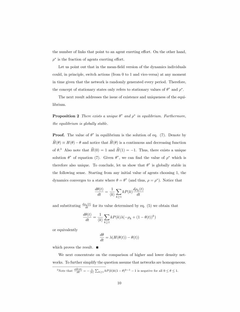
Proposition 2 There exists a unique �� and �� in equilibrium. Furthermore,
the equilibrium is globally stable.
Proof. The value of �� in equilibrium is the solution of eq. (7). Denote byeH(�) � H(�)� � and notice that eH(�) is a continuous and decreasing functionof �.3 Also note that eH(0) = 1 and eH(1) = �1. Thus, there exists a unique
solution �� of equation (7). Given ��, we can �nd the value of �� which is
therefore also unique. To conclude, let us show that �� is globally stable in
the following sense. Starting from any initial value of agents choosing 1, the
dynamics converges to a state where � = �� (and thus, � = ��). Notice that
d�(t)
dt=
1
hkiXk�1
kP (k)d�k(t)
dt
and substituting d�k(t)dt for its value determined by eq. (5) we obtain that
d�(t)
dt=
1
hkiXk�1
kP (k)�(��k + (1� �(t))k)
or equivalentlyd�
dt= �(H(�(t))� �(t))
which proves the result.
We next concentrate on the comparison of higher and lower density net-
works. To further simplify the question assume that networks are homogeneous.
3Note that d eH(�)d�
= � 1hki
Pk�1 kP (k)k(1� �)k�1 � 1 is negative for all 0 � � � 1.
10
That is, all agents have the same connectivity. Let ��(k) and ��(k) represent
the values of � and � in equilibrium when the network is homogeneous and with
connectivity k. The following result holds.
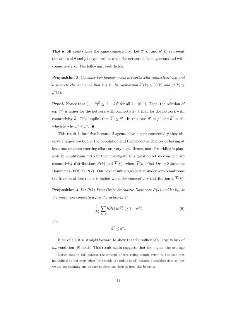
Proposition 3 Consider two homogeneous networks with connectivities k and
k respectively, and such that k � k. In equilibrium ��(k) � ��(k) and ��(k) �
��(k).
Proof. Notice that (1� �)k � (1� �)k for all � 2 [0; 1]. Then, the solution of
eq. (7) is larger for the network with connectivity k than for the network with
connectivity k. This implies that �� � ��. In this case �� = �� and �� = ��,
which is why �� � ��.
This result is intuitive because if agents have higher connectivity they ob-
serve a larger fraction of the population and therefore, the chances of having at
least one neighbor exerting e¤ort are very high. Hence, more free riding is plau-
sible in equilibrium.4 To further investigate this question let us consider two
connectivity distributions P (k) and P (k), where P (k) First Order Stochastic
Dominates (FOSD) P (k). Our next result suggests that under some conditions
the fraction of free riders is higher when the connectivity distribution is P (k).
Proposition 4 Let P (k) First Order Stochastic Dominate P (k) and let km be
the minimum connectivity in the network. If
1
hkiXk�1
kP (k)e�kkm � 1� e
�1km (9)
then
�� � ��.
First of all, it is straightforward to show that for su¢ ciently large values of
km condition (9) holds. This result again suggests that the higher the average
4Notice that in this context the concept of free riding simply refers to the fact that
individuals do not exert e¤ort (or provide the public good) because a neighbor does so, but
we are not claiming any welfare implications derived from this behavior.
11
connectivity in the network the larger the fraction of free riders in the popula-
tion. As formally explained in footnote 5, the order between �� and �� cannot
be precisely established and might depend on additional properties of P (k)
and P (k). However, given the result and intuition derived for homogeneous
networks we conjecture that, in most cases, �� � ��.
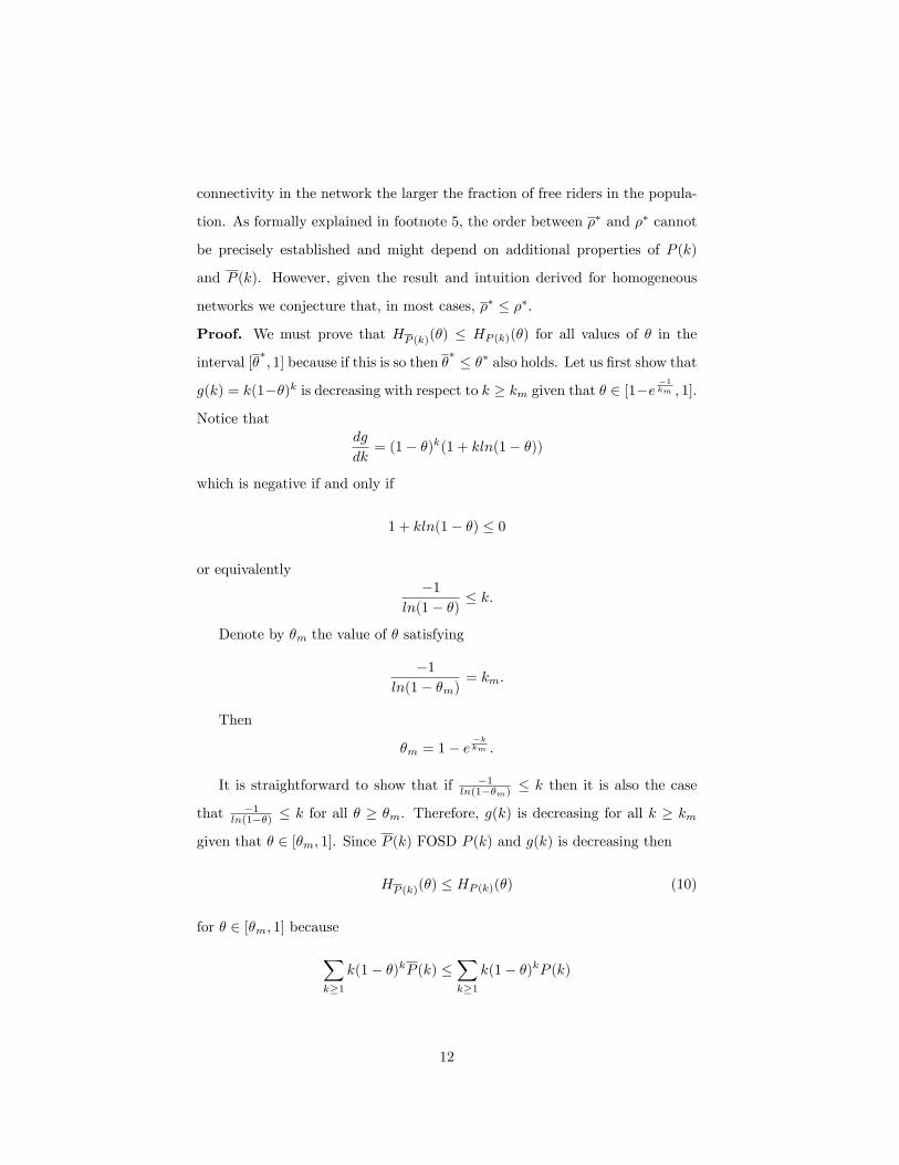
Proof. We must prove that HP (k)(�) � HP (k)(�) for all values of � in the
interval [��; 1] because if this is so then �
� � �� also holds. Let us �rst show that
g(k) = k(1��)k is decreasing with respect to k � km given that � 2 [1�e�1km ; 1].
Notice thatdg
dk= (1� �)k(1 + kln(1� �))
which is negative if and only if
1 + kln(1� �) � 0
or equivalently�1
ln(1� �) � k.
Denote by �m the value of � satisfying
�1ln(1� �m)
= km.
Then
�m = 1� e�kkm .
It is straightforward to show that if �1ln(1��m) � k then it is also the case
that �1ln(1��) � k for all � � �m. Therefore, g(k) is decreasing for all k � km
given that � 2 [�m; 1]. Since P (k) FOSD P (k) and g(k) is decreasing then
HP (k)(�) � HP (k)(�) (10)
for � 2 [�m; 1] becauseXk�1
k(1� �)kP (k) �Xk�1
k(1� �)kP (k)
12
and since hki �k�then
1k� Xk�1
kP (k)(1� �)k � 1
hkiXk�1
kP (k)(1� �)k.
Condition (9) implies that �m < HP (k)(�m) and therefore �m � ��which
in turn implies that condition (10) also holds for � 2 [��; 1]. This completes
the proof.5
Consider two networks with the same average connectivity, but where one
is a Mean Preserving Spread (MPS) of the other. Which network has a larger
fraction of free-riders in equilibrium? The next result partially addresses this
question.
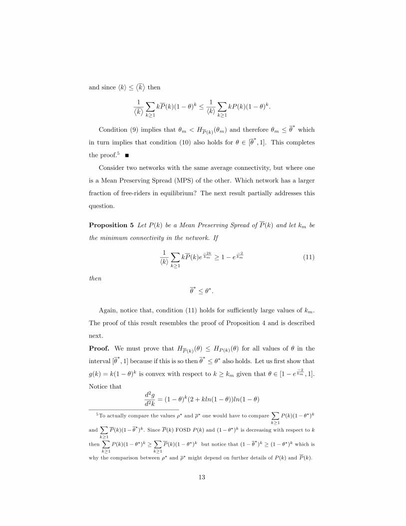
Proposition 5 Let P (k) be a Mean Preserving Spread of P (k) and let km be
the minimum connectivity in the network. If
1
hkiXk�1
kP (k)e�2kkm � 1� e
�2km (11)
then
�� � ��.
Again, notice that, condition (11) holds for su¢ ciently large values of km.
The proof of this result resembles the proof of Proposition 4 and is described
next.
Proof. We must prove that HP (k)(�) � HP (k)(�) for all values of � in the
interval [��; 1] because if this is so then �
� � �� also holds. Let us �rst show that
g(k) = k(1� �)k is convex with respect to k � km given that � 2 [1� e�2km ; 1].
Notice thatd2g
d2k= (1� �)k(2 + kln(1� �))ln(1� �)
5To actually compare the values �� and �� one would have to compareXk�1
P (k)(1� ��)k
andXk�1
P (k)(1� ��)k. Since P (k) FOSD P (k) and (1� ��)k is decreasing with respect to k
thenXk�1
P (k)(1� ��)k �Xk�1
P (k)(1� ��)k but notice that (1� ��)k � (1� ��)k which is
why the comparison between �� and �� might depend on further details of P (k) and P (k).
13
which is positive if and only if
2 + kln(1� �) � 0
or equivalently�2
ln(1� �) � k.
Denote by �m the value of � satisfying
�2ln(1� �m)
= km.
Then
�m = 1� e�2kkm .
It is straightforward to show that if �2ln(1��m) � k then it is also the case
that �2ln(1��) � k for all � � �m. Therefore, g(k) is convex for all k � km given
that � 2 [�m; 1]. Since P (k) is a MPS of P (k) and g(k) is convex then
HP (k)(�) � HP (k)(�) (12)
for � 2 [�m; 1]. Condition (11) implies that �m < HP (k)(�m) and therefore
�m � ��which in turn implies that condition (12) holds also for � 2 [��; 1].
This completes the proof.6
We conjecture that generally �� and �� are aligned in the sense that if
�� (��) is higher for one connectivity distribution than for another, so is ��
(��). We have not been able to show this analytically which is why we study
some examples in the next section. However, the intuition for why the fraction
of agents exerting e¤ort is higher in high-variance networks (provided that
�� is also high for high variance networks as proved in Proposition 5) is the
following. Notice that a high variance network has a signi�cant number of hubs
6To actually compare the values �� and �� one would have to compareXk�1
P (k)(1� ��)k
andXk�1
P (k)(1� ��)k. Since P (k) is a MPS of P (k) and (1� ��)k is convex with respect to
k thenXk�1
P (k)(1� ��)k �Xk�1
P (k)(1� ��)k but notice that (1� ��)k � (1� ��)k which is
why the comparison between �� and �� might depend on further details of P (k) and P (k).
14

(i.e., nodes with very high connectivity) and a signi�cant fraction of nodes with
low connectivity. Thus, there are high chances that a low connectivity node
ends up connected with a high connectivity node. Obviously high connectivity
nodes are going to often free ride from one of their neighbors and therefore often
choose 0, whereas the peripheral agents connected to them would often choose
1. Given Proposition 5, the number of links pointing to an agent choosing 1 is
higher in a high variance network, therefore the only way �� could be reversed
(i.e., higher for low variance networks) would be if the hubs of the high variance
networks are the ones exerting e¤ort. Nevertheless, this is not generally going
to be the case given the argument stated above.
3.3 An Example
Consider networks where agents are of two types: high connectivity agents and
low connectivity agents. In particular, assume that m is the average connec-
tivity of the network and the connectivity distribution is given by:
Pm;v(k) =
8<:12 if k = m+ v
12 if k = m� v
(13)
where v indicates how far from the mean are the two connectivities. We sub-
stitute this connectivity distribution in eq.(7) and (8) to analyze the collective
outcomes for di¤erent values of the parameters m and v determine. We con-
centrate on the question of how the variance of the connectivity distribution
determines the fraction of free riders in equilibrium. To do so, we consider a
�xed value of m and observe what happens with the equilibrium outcome as
v takes values from 0 to approximately m � 1. In �g.1 we represent the frac-
tion of agents exerting e¤ort in equilibrium �� as a function of v. Each graph
represents a di¤erent value for the average connectivity (m = 10, m = 100
and m = 1000, in the �rst, second and third graph respectively). Notice that
qualitatively all curves are very similar. That is, the higher the variance of the
network (higher v) the higher the fraction of agents choosing 1 and thus the
15
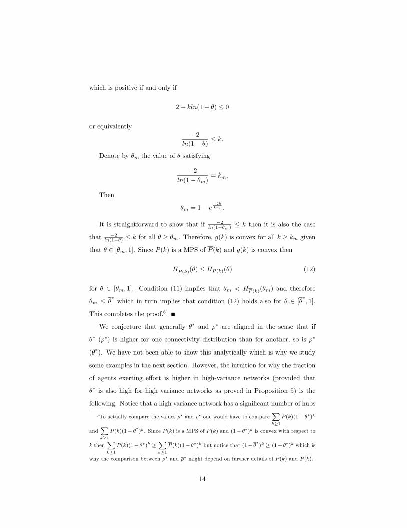
Figure 1: Representation of the fraction of agents exerting e¤ort in equilibrium
(��) as a function of v, for the values of m = 10, m = 100 and m = 1000.
lower the fraction of free-riders. Also, comparing one graph with the other, we
�nd that going from a low to a high average connectivity network decreases the
number of agents exerting e¤ort and thus increases the fraction of free riders.
One can also show that if instead of equilibrium value of �� we represent
the equilibrium value of �� the graphs look roughly the same.
4 Simulations
In this section we investigate the role of the variance of the connectivity dis-
tribution on the fraction of free riders through simulations of the dynamics on
�xed networks. We generate two di¤erent random networks in terms of their
connectivity distributions:7 (i) a scale-free network with connectivity distribu-
tion P (k) / k�2:5 for k � 3 and PSF (k) = 0 otherwise (where / means, equal
up to a multiplicative constant) (ii) an exponential network P (k) / e�k6 for
k � 3 and PE(k) = 0 otherwise.8 Each of these two networks have a total of
1000 nodes and an average connectivity of approximately 9, however, scale-free
networks have signi�cantly larger variance than exponential networks. The in-
7The main reason why the dynamics on random networks might reproduce the mean-
�eld approximations is that in a random network the characteristics of any given node is
una¤ected by structural correlations.8These networks were generated using the program Pajek, a software package for Large
Network Analysis.
16
terest in the study of scale-free networks is enhanced by the empirical evidence
that many paradigmatic examples of complex networks such as the WWW and
the human sexual contact network, among others, are characterized by scale-
free connectivity properties (see e.g., Barabasi et al., 2000 and Lijeros et al.,
2001).
We consider the discrete version of the continuous dynamics used to derive
the theoretical results. In this respect, we assume that, in every period one (and
only one) agent is chosen to revise his strategy and chooses action 1 if and only
if none of his neighbors doing so. The network remains �xed throughout the
dynamics which marks a crucial di¤erence between the mean-�eld approach
and the simulation.
In �g. 2 below we represent the number of agents exerting e¤ort (or public
good providers, PGP) as a function of time, where 1 � t � 10000 for the
scale-free network (red) and the exponential network (blue). We considered
two di¤erent initial conditions; one where the number of PGP is 0 and the
other where this number is 1000 (i.e., all agents are initially choosing action 1).
Although for clarity in the graph we have simply represented a sample of 12
simulations per network, we have obtained the same convergence result when
considering a sample size of 100.
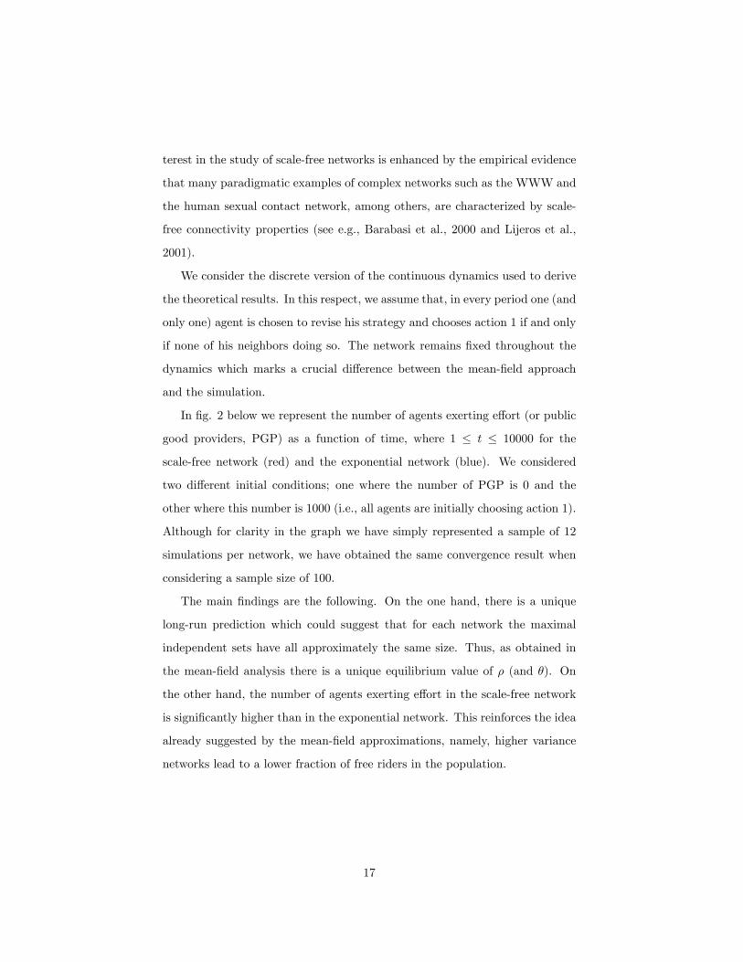
The main �ndings are the following. On the one hand, there is a unique
long-run prediction which could suggest that for each network the maximal
independent sets have all approximately the same size. Thus, as obtained in
the mean-�eld analysis there is a unique equilibrium value of � (and �). On
the other hand, the number of agents exerting e¤ort in the scale-free network
is signi�cantly higher than in the exponential network. This reinforces the idea
already suggested by the mean-�eld approximations, namely, higher variance
networks lead to a lower fraction of free riders in the population.
17
Figure 2: Representation of the number of agents exerting e¤ort � (or public
good providers, PGP) as a function of time 1 � t � 10000 for a scale-free
(SF, red in the graph) and an exponential (Exp, blue in the graph) network.
The number of simulations are 12 per network and half start with an initial
condition of �0 = 0 and half with an initial condition of �0 = 1.
18
5 Discussion
It is well known that the outcomes of many socioeconomic phenomena cru-
cially depend on the properties of the social networks in which the agents are
embedded. Some paradigmatic examples of processes where the social network
is relevant are the di¤usion of a new technology (e.g., Lopez-Pintado, 2004,
2006, Jackson and Yariv, 2006), the spread of information on job opportuni-
ties (e.g., Calvo-Armengol and Jackson, 2006), the uprising of political revolts
(e.g., Chwe, 2000), or even the di¤usion of an infectious disease (e.g., Pastor-
Satorras and Vespignani, 2001). Whereas in most of this literature the behavior
(or states) propagate in such a way that the more agents adopting the behavior
the more it spreads, this paper studies a stylized model of precisely the polar
case. That is, we study a process where agents want to anti-coordinate with
their neighbors.
There are a few other papers that analyze this problem theoretically. For in-
stance, Bramoulle (2007) addresses the case of anti-coordination games played
among agents connected in a social network. Apart from the methodology used,
the model proposed in Bramoulle (2007) di¤ers from the model considered in
this paper because he assumes that agents adopt an action whenever less than
a certain fraction of their neighbors is doing so, whereas here we assume that
one neighbor alone generates enough incentives to free ride.
Bramoulle and Kranton (2006) is perhaps the closest paper to this work, as
they also analyze local public goods in terms of e¤ort decisions among agents
in a network. The main di¤erences between their model and the model studied
here are the following. First, Bramoulle and Kranton (2006) assume that agents
choose a level of e¤ort which is a continuous decision instead of a binary one.
Second, Bramoulle and Kranton (2006) propose a utility function for each agent
with the feature that the bene�ts each agent obtains from interacting with his
neighbors are a concave function of the total level of e¤ort exerted in the agent�s
neighborhood. In our model, the utility function is not necessarily concave on
19
bene�ts, but nevertheless we make the assumption that agents would only want
to exert e¤ort if no other neighbor does so, which in some sense restricts the
problem even further. One of the disadvantages of not specifying the utility
function is that we cannot engage in welfare comparisons of the equilibrium
outcomes. The main novelty of our approach, however, is the methodology
used in order to address questions that otherwise would be intractable. The
mean-�eld approximations simplify the problem in a way so that we are able
to compare network structures in terms of the properties of their connectivity
distributions.
Finally, it is worth commenting on other works dealing with mean-�eld
approximations of a network model such as Pastor-Satorras and Vespignani
(2001), Lopez-Pintado (2004, 2006), Jackson and Yariv (2006), Rogers and
Jackson (2007), etc. Most of these papers concentrate on the case where
agents become more susceptible to a certain action the more neighbors adopt
it. Lopez-Pintado (2004) studies a family of contagion processes with this fea-
ture, whereas Lopez-Pintado (2006) concentrates on a speci�c context where
agents play a coordination game with each neighbor. Finally, Jackson and Yariv
(2006) introduce a general di¤usion of behavior model where not only coordi-
nation but also anti-coordination processes are considered. The current paper,
however, can be viewed as a more detailed analysis of a speci�c scenario. It
is worth mentioning that as Jackson and Yariv (2006) explain, the equilibrium
outcomes of the mean-�eld dynamics could also be thought of as the symmetric
Bayesian equilibrium outcomes of a Bayesian game where agents, characterized
by their connectivities (types), simultaneously choose their actions knowing the
connectivity distribution in the population, and assuming that connectivities
are independently allocated throughout the network (see also Galeotti et al.,
2005 for another use of this same approach).
20
References
[1] Benaim M. and J. Weibull, "Deterministic Approximation of Stochastic
Evolution in Games", (2003) Econometrica 71, 873-903.
[2] Barabasi A., Albert R. and H. Jeong, "Scale-free Characteristics of Ran-
dom Networks: the Topology of the World-Wide Web", (2000) Physica A
281, 2115.
[3] Bramoulle Y. and R. Kranton, "Public Goods in Networks" (2006) Journal
of Economic Theory, forthcoming.
[4] Bramoulle Y., "Anti-Coordination Games and Social Interactions", (2007)
Games and Economic Behavior 58, 30-49.
[5] Calvo-Armengol A. and M. Jackson, "The E¤ects of Social Networks on
Employment and Inequality" (2004), American Economic Review 94 (3),
426-454.
[6] Chwe M. S-Y., "Communication and Coordination in Social Networks",
(2000) The Review of Economic Studies 67, 1-16.
[7] Galeotti A., Goyal S., Jackson M. O., Vega-Redondo F. and L. Yariv,
"Network Games", (2005) mimeo.
[8] Jackson M. O. and B. Rogers, "Relating Network Structures to Di¤usion
Properties through Stochastic Dominance", (2007) The B. E. Journal of
Theoretical Economics 7(1) (Advances), 6.
[9] Jackson M.O. and L. Yariv, "Di¤usion of Behavior and Equilibrium Prop-
erties in Network Games", (2006) American Economic Review (Papers
and Proceedings), forthcoming.
[10] Lijeros F., Edling C. R., Amaral L. A. N., Stanley H. E., and Y. Aberg,
"The Web of Human Sexual Contacts", (2001) Nature 441, 907-908.
21
[11] Lopez-Pintado D., "Contagion and Coordination in Random Networks",
(2006) International Journal of Game Theory 34, 371-381.
[12] Lopez-Pintado D., "Di¤usion in Complex Networks", (2004) IVIE WP-AD
2004-33, Universidad de Alicante.
[13] Pastor-Satorras P. and A. Vespignani, "Epidemic Dynamics and Endemic
States in Complex Networks", (2001) Physical Review E 63, 066117.
22