The spectrum of thallium chloride 249 - Royal Societyrspa.royalsocietypublishing.org/content/royprsa/166/925/249.full.pdf · (xrp){A'...)pp,rJf{xrp’)^dT1...dTr

$Page 1: The spectrum of thallium chloride 249 - Royal Societyrspa.royalsocietypublishing.org/content/royprsa/166/925/249.full.pdf · (xrp){A'...)pp,rJf{xrp’)^dT1...dTr$
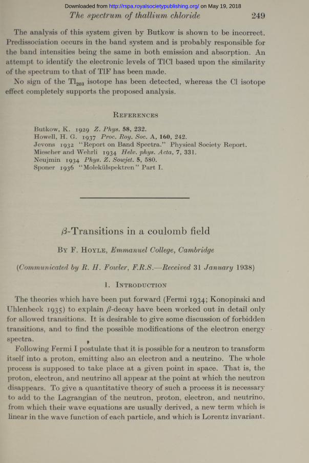
The spectrum of thallium chloride 249

The analysis of this system given by Butkow is shown to be incorrect. Predissociation occurs in the band system and is probably responsible for the band intensities being the same in both emission and absorption. An attempt to identify the electronic levels of T1C1 based upon the similarity of the spectrum to that of T1F has been made.

No sign of the Tl203 isotope has been detected, whereas the Cl isotope effect completely supports the proposed analysis.

R e f e r e n c e s

Butkow, K. 1929 Z. Phys. 58, 232.Howell, H. G. 1937 Proc. Boy. Soc. A , 160 , 242.Jevons 1932 “ R eport on B and Spectra .” Physical Society R eport. Miescher and W ehrli 1934 Helv. phys. Acta, 7, 331.Neujm in 1934 Phys. Z . Sowjet. 5, 580.Sponer 1936 “ M olekiilspektren ” P a r t I.

-T ransitions in a coulomb field

B y F. H o y l e , Emmanuel College, Cambridge

[Communicated by R. 11. Fowler, F.R—Received 31 January 1938)

1. I n t r o d u c t io n

The theories which have been put forward (Fermi 1934; Konopinski and Uhlenbeck 1935) to explain /?-decay have been worked out in detail only for allowed transitions. It is desirable to give some discussion of forbidden transitions, and to find the possible modifications of the electron energy spectra. f

Following Fermi I postulate that it is possible for a neutron to transform itself into a proton, emitting also an electron and a neutrino. The whole process is supposed to take place at a given point in space. That is, the proton, electron, and neutrino all appear at the point at which the neutron disappears. To give a quantitative theory of such a process it is necessary to add to the Lagrangian of the neutron, proton, electron, and neutrino, from which their wave equations are usually derived, a new term which is linear in the wave function of each particle, and which is Lorentz invariant.

on May 19, 2018http://rspa.royalsocietypublishing.org/Downloaded from

http://rspa.royalsocietypublishing.org/

250 F. Hoyle

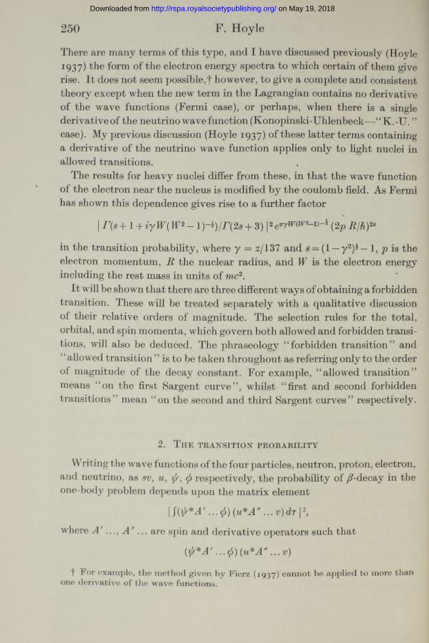
There are many terms of this type, and I have discussed previously (Hoyle 1937) the form of the electron energy spectra to which certain of them give rise. It does not seem possible,f however, to give a complete and consistent theory except when the new term in the Lagrangian contains no derivative of the wave functions (Fermi case), or perhaps, when there is a single derivative of the neutrino wave function (Konopinski-Uhlenbeck—“ K.-U. ” case). My previous discussion (Hoyle 1937) of these latter terms containing a derivative of the neutrino wave function applies only to light nuclei in allowed transitions.

The results for heavy nuclei differ from these, in that the wave function of the electron near the nucleus is modified by the coulomb field. As Fermi has shown this dependence gives rise to a further factor

I r (s+ l+ iy W (W 2- 1 )-*) / r (2s + 3) 12 (2p

in the transition probability, where y = 2/137 and s — (1 — y2)* — 1, p is the electron momentum, R the nuclear radius, and W is the electron energy including the rest mass in units of me2.

It will be shown that there are three different ways of obtaining a forbidden transition. These will be treated separately with a qualitative discussion of their relative orders of magnitude. The selection rules for the total, orbital, and spin momenta, which govern both allowed and forbidden transitions, will also be deduced. The phraseology “ forbidden transition” and “ allowed transition ” is to be taken throughout as referring only to the order of magnitude of the decay constant. For example, “ allowed transition” means ” on the first Sargent curve”, whilst “ first and second forbidden transitions” mean “ on the second and third Sargent curves” respectively.

2. T h e t r a n sit io n p r o b a b il it y

Writing the wave functions of the four particles, neutron, proton, electron, and neutrino, as sv, u, ijs, (jj respectively, the probability of /?-decay in the one-body problem depends upon the matrix element

|J(f*A '...0 )(^*A "...v )dT |2,

where A '..., A"... are spin and derivative operators such that

(ft* A ' ... ft)( ...v)

f For example, the m ethod given by Fierz (1937) cannot be applied to more than one derivative of the wave functions.



ft-Transitions in a coulomb field 251

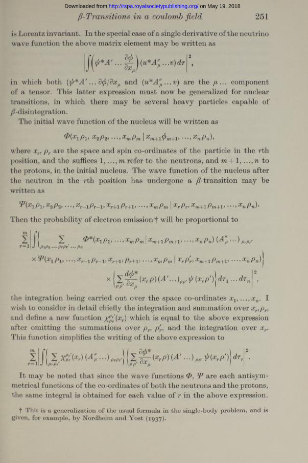
is Lorentz invariant. In the special case of a single derivative of the neutrino wave function the above matrix element may be written as

in which both (i/r*A'... dtfi/dx and {u*A"u...v) are the f t ... componentof a tensor. This latter expression must now be generalized for nuclear transitions, in which there may be several heavy particles capable of /^-disintegration.

The initial wave function of the nucleus will be written as

0 (x1p1, x2p2, ...,xmpm xm+l<f>m+l’ *••>

where xr, pr are the space and spin co-ordinates of the particle in the rth position, and the suffices 1 , ...,mrefer to the neutrons, and m + 1, tothe protons, in the initial nucleus. The wave function of the nucleus after the neutron in the rth position has undergone a /^-transition may be written as

T(XiPi,X2p2, ..., Xr_iPr_i, xr+lPr+l’ •••> # I •••> )•

Then the probability of electron emission f will be proportional tomir= 1

^ 0 ( *1 • • • ? Xmpm j Pm+1> * • * ? XnPn) * * * ) prprJ \P1P2 • • • Prpr • • • pn

X ? Xr—1 Pr—1> V-Kl? Pr+1> •••’XmPm I XrPr> Xm+1 Pm+1’ • • • 3

^ d<$>*pp'

(xrp){A'...)pp,rJf{xrp’)^dT1 ...dTr

the integration being carried out over the space co-ordinates xv ...,xn. I wish to consider in detail chiefly the integration and summation over xr,pr, and define a new function Xpr(xr)which is equal to the above expression after omitting the summations over pr, p'r, and the integration over xr. This function simplifies the writing of the above expression to

r= 1 J \prPr2 Xpr'(xr) P rP r 2 ^ - ( XrP)(A> ■pp' UU/p

) P P ' f { x rp')

It may be noted that since the wave functions O, W are each antisym- metrical functions of the co-ordinates of both the neutrons and the protons, the same integral is obtained for each value of r in the above expression.

t This is a generalization of the usual formula in the single-body problem, and is given, for example, by Nordheim and Yost (1937).



252 F. Hoyle

The neutrino is a free particle, and the form of its eigen states of linear momentum are known, but before discussing the properties of the integral the positive energy solutions ft(x,p) of the electron wave equation are also required. A summary of the properties of such solutions is given in the Appendix, the full details having been discussed, for example, by Hulme(I931)-

3. A l lo w e d a nd f o r b id d e n t r a n sit io n s

The components of the function Xpr(xr)may be expected to have different orders of magnitude. This would arise in a similar way to the small components in the Pauli reduction of the Dirac equation for a single slow- moving particle (Bethe 1933, p. 304). In this case thep = 1, 2 components differ from the p = 3,4 components by a factor which is of order vfc, which taking v as the velocity of a nuclear particle is about 1/10. Now if it is assumed that a relativistic equation can be formulated for the whole nucleus, each spin co-ordinate having the values 1, 2, 3, 4, 1 expect a similar reduction to a non-relativistic Schrodinger equation, in which the only components of 0 , ¥ which occur will be those in which every spin coordinate is 3, 4. I t is useful to consider the analogy with the case of a single heavy particle still further. One knows, in this latter case, that if one expresses the small components in terms of the large components, then the contribution of largest order is from the space derivatives of the large components. These space derivatives give the factor v/c. I wish to take over this result for the different components of the nuclear wave functions 0 , ¥ when the value of a given pis changed from 3, 4 to 1, 2 (all other spin co-ordinates having values 3, 4).

That is, if 0 ', 0 " are written for the components of 0 when the particular p has the values 1, 2, and 3, 4, respectively, all other p’s having values, 3, 4, I assume that we shall then have a relation, which is, to the first order of approximation in the ratio of 0 ', 0" ,

1 > ' = 1 (<rkP„)4>",k = 1

where er kare the Pauli matrices, and Pk is the analogue of \mc2(djdxk + eAk) in the single-body problem A k being the vector potential (Bethe 1933’ P- 3°5’ eqii- 8*4). There will be a similar relation for the components of the wave function ¥, and if we make similar definitions this will be

¥"= i ( o - kQk = 1




where Qk is similar, but not identical, to I t will be of importance later tonotice that the operators Pk, Qk, may be supposed to change sign, with a change of sign of the space co-ordinates. I t is now expected that if in the relativistic equations of motion for the nucleus all components of the wave function which have any spin co-ordinate except different from 3, 4 are neglected, and if I approximate further by using a first-order expression (of the type given for 0',W) when/?r =1 ,2 , then thepr = 3, 4 components will have the same space distribution. That is, for this approximation the spin dependence upon pr is independent of the space dependence upon xr. This approximation is termed “ neglecting spin forces”, and this case is to be regarded as giving the first approximation. In treating the second approximation it is necessary to consider, for example, both the second-order terms in the above expressions for 0 ', W, and also the first-order terms in the expressions for the components of 0 ,W, in which two spin co-ordinates have the values 1,2.

I shall confine myself to a discussion of the first approximation, treating first the case in which pr is the spin variable of the particle making the transition. This is a special case, since the spin co-ordinate of the transition particle is operated upon by A " ... in our matrix element. The summation, in the matrix element, over all spin co-ordinates except will now be only over the values 3, 4. The product function will have 16 componentsof which we regard 4 as “ large”, 8 components will differ from the “ large” components by a factor of order yy, whilst 4 components will differ by a factor of order y^y. These will be

Xprr=l’,i(xr)the ‘ ‘ large ’ ’ components;Xp'r =l’Mxr)and Xpr=l’,t(xr) differing by a factor of order yL;

Xpr=i,l(xr) differing by a factor of order y ^ .

Each of the functions XPr(xr)can he expanded in a series of spherical harmonics. In the integration of these functions over the co-ordinates xr a result which differs from zero will be obtained only from the spherical harmonic which is of the same order as the spherical harmonic given by the wave functions of the light particles. Now it is known that the light particle wave functions which have different spherical harmonic dependences have different orders of magnitude near the nucleus. The results required for these wave functions can be written down from the Appendix.

If I treat the light particle wave functions as constants, then I take 6r0, P-i-i for the electron, and consider the neutrino wave function as constant over the nucleus. The form of the electron energy spectrum depends only



254 F. Hoyle

upon the form of the electron and neutrino wave functions, and this case gives a distribution which will be termed the “ allowed distribution form” This is

A\r(s+\+iyW(W*~ l)-*)/F(2s + 3) (2pBjh)»x W{W*-l)t(WQ-W)*.

The value of A will depend upon which component of Is considered.Distributions of this type are obtained for all components, but A will have different orders of magnitude in accordance with the different orders of magnitude of the components of X%(xr)-

If now only a first-order harmonic, cos 6 say, from the light particles, will give an integral different from zero, there are three ways of obtaining such a cos 6 dependence:

(1) Take F0, G_x_x for the electron, and consider the neutrino as constant over the nucleus. We shall obtain a distribution which is of the “ allowed form”, but the transition probability will contain a factor of order Jy2.

(2) Take Gx, F_2_1 for the electron and again consider the neutrino as constant over the nucleus. The electron energy distribution will now differ from the allowed form by an extra factor ( — 1), whilst the decay constant will be decreased by a factor of order (îo)2-

(3) Lastly, take G0, F_x_xfor the electron and consider the first-order variation of the neutrino wave function over the nucleus. This gives a distribution which differs from the allowed form by a factor (W0 IT)2, and the decay constant is decreased by a factor (4V)2 (Bethe and Bacher 1936, p. 195).

It is noted that the selection rules for these three cases will be identical, and that it is necessary to compare the orders of magnitude of the decay constants given by each case. It is convenient to write the second and third cases together as giving a distribution

(i^)2 x {“ allowed distribution”) x 1) W)2},

where a,b are at most of order unity. This we call the ‘ ‘ first modified form ’ ’. It will only be comparable in magnitude with the first case when y is very small, that is, for very light (z 20) elements. This point is, however,dependent upon treating the solutions of the electron wave equation, which assumes the nucleus to act like a point charge, as a good approximation even for radii of nuclear dimensions.

There are again many possibilities if I require the possible light particle



f$- Transitions in a coulomb field 255

wave functions which give a second-order spherical harmonic, cos say. These are:

(1) Take Fv G_2-i> and treat the neutrino wave function as constant.(2) Take F0, G_±_v and the first-order variation of the neutrino wave

function over the nucleus.(3) Take G2,F_3_l5 and treat the neutrino wave function as constant.(4) Take Q1,F_t_1 , and the first-order variation of the neutrino wave

function over the nucleus.(5) Take G0, F_±_v and the second-order variation of the neutrino wave

function over the nucleus.Each of these possibilities will again have the same selection rules, and it

is necessary to compare their orders of magnitude. If I take 3, 4, and 5 together I obtain approximately a distribution

(^ )4 x (“ allowed distribution”)x {a( W‘2 - 1 )2 + b( W‘2 - 1) ( + c(W0 - W)*},

where a, b, c are at most of order unity. This distribution is termed the “ second modified form” . Taking 1, 2 together gives

ly 2 ) 2 x (“allowed distribution ”} x {a( W2 — 1) -f b(WQ — IF)2},

where a, b are again at most of order unity. I t can be seen that 1, 2 give the “ first modified form ”, and that this will be the effective distribution except for very light elements.

The three cases where zero-, first-, and second-order spherical harmonics are taken from the wave functions of the light particles are separately considered, and it is seen that they lead not only to transition probabilities with different orders of magnitude, but also to different possible electron energy distributions. It is therefore convenient in discussing the selection rules obtained from the different components of ) to treat these threecases separately, since if it is supposed that for any component there is the same selection rule in two different cases (for example, in both the case where we consider the wave functions of the light particles as constants, and where they give a cos 6 angular dependence), then the only case that need be considered is that which gives the largest transition probability, that is, the case in which the light particle wave functions give the spherical harmonic of least order.

To determine the selection rules for these various transitions it is necessary



256 F. Hoyle

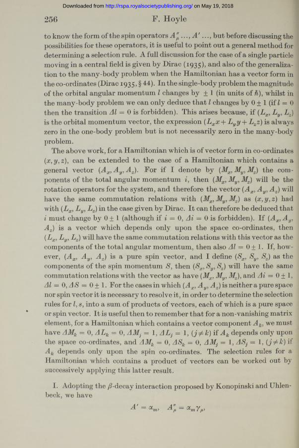
to know the form of the spin operators " ..., . but before discussing thepossibilities for these operators, it is useful to point out a general method for determining a selection rule. A full discussion for the case of a single particle moving in a central field is given by Dirac (1935), and also of the generalization to the many-body problem when the Hamiltonian has a vector form in the co-ordinates (Dirac 1935, § 44). In the single-body problem the magnitude of the orbital angular momentum l changes by ± 1 (in units of whilst in the many-body problem we can only deduce that l changes by 0 + 1 (if = 0 then the transition Al = 0 is forbidden). This arises because, if ( L z)is the orbital momentum vector, the expression is alwayszero in the one-body problem but is not necessarily zero in the many-body problem.

The above work, for a Hamiltonian which is of vector form in co-ordinates (x,y,z), can be extended to the case of a Hamiltonian which contains a general vector (Ax, A y, A z).For if I denote by the components of the total angular momentum then My, Mz) will be the rotation operators for the system, and therefore the vector ( , A y, ) willhave the same commutation relations with (Mx,My,Mz) as hadwith ( L x , L y, L z) in the case given by Dirac. I t can therefore be deduced that i must change by 0 ± 1 (although if i = 0, = 0 is forbidden). If A z) is a vector which depends only upon the space co-ordinates, then ( L x , L y, L z) will have the same commutation relations with this vector as the components of the total angular momentum, then also 0 ± 1. If, however, (Ax, A y, Az) is a pure spin vector, and I define Sy, ) as the components of the spin momentum S, then Sy, Sz) will have the same commutation relations with the vector as have (Mx Mz), and = 0 + 1, Al = 0,AS = Q ± 1. For the cases in which (Ax, A y, A z)is neither a pure space nor spin vector it is necessary to resolve it, in order to determine the selection rules for l, s, into a sum of products of vectors, each of which is a pure space or spin vector. I t is useful then to remember that for a non-vanishing matrix element, for a Hamiltonian which contains a vector component A k, we must have AMk = 0, ALk = 0, AM} = 1, ALj = 1, 0V if A k depends only uponthe space co-ordinates, and AMk = 0, ASk = 0, 1 1, (j¥=k) if A k depends only upon the spin co-ordinates. The selection rules for a Hamiltonian which contains a product of vectors can be worked out by successively applying this latter result.

I. Adopting the /?-decay interaction proposed by Konopinski and Uhlen- beck, we have

■1



257

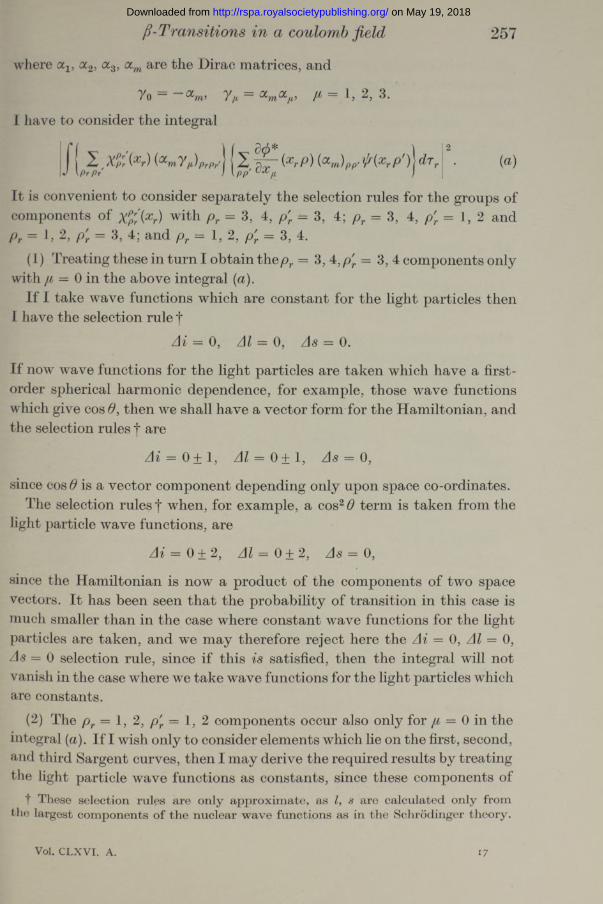
where a l5 a2, oc3, <xmare the Dirac matrices, and

7 o = _ a m) 7 / t = a /n a /<J = h

I have to consider the integral

j ^ 'Xpr(**V) (am7 /<)pr/>/| 12 farP) (&m) pp'ftfar P ) j j • (a )

It is convenient to consider separately the selection rules for the groups of components of x%(xr) with Pr = 4, Pr = 3> 4 ; = 3, 4, = 1, 2 andpr = 1, 2, p'r = 3, 4 ; and pr — 1, 2, p' = 3, 4.

(1) Treating these in turn I obtain the = 3, 4, = 3,4 components onlywith p = 0 in the above integral (a).

If I take wave functions which are constant for the light particles then I have the selection rule f

Ai = 0, Al = 0, As = 0.

If now wave functions for the light particles are taken which have a first- order spherical harmonic dependence, for example, those wave functions which give cos 6 , then we shall have a vector form for the Hamiltonian, and the selection rules f are

Ai = 0+ 1, Al = 0+ 1, As = 0,

since cos 6 is a vector component depending only upon space co-ordinates.The selection rules f when, for example, a cos2 6 term is taken from the

light particle wrave functions, are

Ai = 0 + 2, Al — 0 + 2, As = 0,

since the Hamiltonian is now a product of the components of two space vectors. I t has been seen that the probability of transition in this case is much smaller than in the case where constant wave functions for the light particles are taken, and we may therefore reject here the 0, = 0,As = 0 selection rule, since if this is satisfied, then the integral will not vanish in the case where we take wave functions for the light particles which are constants.

(2) The pr = 1, 2, p'r = 1,2 components occur also only for = 0 in the integral (a). If I wish only to consider elements which lie on the first, second, and third Sargent curves, then I may derive the required results by treating the light particle wave functions as constants, since these components of

t These selection rules are only approxim ate, as l, s are calculated only from the largest components of the nuclear wave functions as in the Schrodinger theory.

ft-Transitions in a coulomb field

Vol. CLXVI. A. 17



258 F. Hoyle

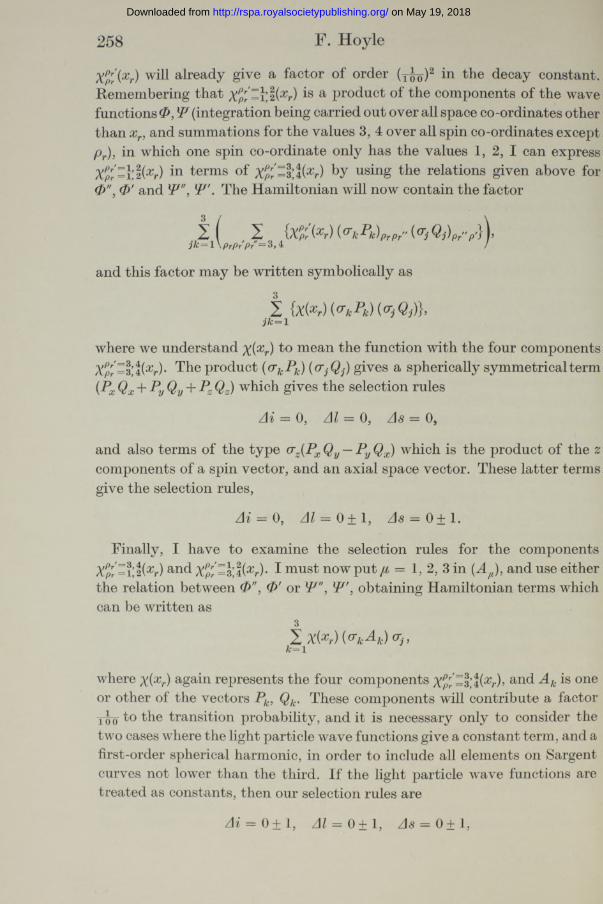
X%(xr) will already give a factor of order (t£q)2 in the decay constant. Remembering that XpPrr=\’.IMis a product of the components of the wave functions 0 , W (integration being carried out over all space co-ordinates other than xr, and summations for the values 3, 4 over all spin co-ordinates except pr), in which one spin co-ordinate only has the values 1, 2, I can express XpPrr=\’\{xr) in terms of XPr=l’,t(xr) by using the relations given above for 0 ", 0 ' and W , W . The Hamiltonian will now contain the factor

I ( I {X^(Xr) ^ k ( < T jj k = l \prp /pr"=S,4:

and this factor may be written symbolically as

2 {X{xr)(<rkPk){<*jQj)}>jk = 1

where we understand X(xr) to mean the function with the four components XPprr=\’,\{xr)' The product (crkPk) gives a spherically symmetrical term(Px Qx + PyQy + Pz Qz) which gives the selection rules

Ai= 0 , Al = 0 , As 0 ,

and also terms of the type <JZ(PX Qy — Py Qx) which is the product of the z components of a spin vector, and an axial space vector. These latter terms give the selection rules,

Ai = 0, Al — 0 ± 1, zls = 0 ± l .

Finally, I have to examine the selection rules for the components XpPi=\ ’,Uxr) an(i Xpf=l’,l (xr)-I must nowput 1, 2, 3 in (HJ, and use either

the relation between 0 ", 0 ' or 0 ", W, obtaining Hamiltonian terms which can be written as

32 X(Xr) (O’fc'dfc) Oy ,k= 1

where x(xr) again represents the four components an( A Is oneor other of the vectors Pk, Qk. These components will contribute a factor

to the transition probability, and it is necessary only to consider the two cases where the light particle wave functions give a constant term, and a first-order spherical harmonic, in order to include all elements on Sargent curves not lower than the third. If the light particle wave functions are treated as constants, then our selection rules are

Ai = 0+1, Al = 0+1, Zl<s = 0+1



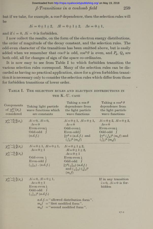
but if we take, for example, a cos 6 dependence, then the selection rules will be

zh' = 0 + 1 ± 2, zl? = 0 + 1 + 2, zls = 0 + 1,

and if i = 0, Ai = 0 is forbidden.I now collect the results, on the form of the electron energy distributions,

the order of magnitude of the decay constant, and the selection rules. The odd-even character of the transitions has been omitted above, but is easily added when we remember that cos 6 is odd, cos2 6 is even, and Pk, Qk are both odd, all for changes of sign of the space co-ordinates.

It is now easy to see from Table I to which forbidden transition the various selection rules correspond. Many of the selection rules can be discarded as having no practical application, since for a given forbidden transition it is necessary only to consider the selection rules which differ from those for forbidden transitions of lower order.

/?- Transitions in a coulomb field 259

T a b le I. T h e s e l e c t io n r u l e s a n d e l e c t r o n d is t r ib u t io n s in

THE K .-U . CASE

Components

Ofconsidered

Taking light particle wave functions which

are constants

Taking a cos 6 dependence from th e light particle wave functions

Taking a cos2 6 dependence from the light particle wave functions

x pP:~ l: i ( x r) A i - 0, Al= 0, A i - 0 ± 1, zlZ = 0 ± 1, zb" = 0 + 2, zlZ = 0 + 2,d s = 0 As = 0 As = 0

Even-even) Odd-even) Even-even)Odd-odd / E v en -o d d / Odd-odd /(a.d.f.) f y 2 x (a .d .f.)and I r 2 (A )2 (mJ ) and

(tV)S ( » * i / ) (to)4 (m2/)

x pPrr= l:K x r)

X%'=l’M Xr)

zh = 0 ± 1, 0 ± 1,As = 0 ± 1

Odd-even ) Even-odd /(tfo ) • (a 'd-f')

A i - 0 ± 1 ± 2 , zlZ = 0 ± 1 ± 2, As = 0 ± 1

E v en-even) Odd-odd / i y 2(iiro) (a -d-f-)

and (jj}q) (j o )2 (% /)

Xprr= i’2(x r) d i = 0, Al= 0 ± 1, I f in any transition As = 0 ± 1 = 0, = 0 is for-

E ven-even) biddenOdd-odd /

a.d.f. = “ allowed distribution fo rm ” . m xf — ‘ ‘ first modified form ’ ’.

m2 f = ‘ ‘ second modified form ’ ’.1 7 - 2



260

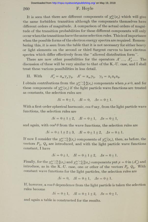
It is seen that there are different components of which will givethe same forbidden transition although the components themselves have different orders of magnitude. A comparison of the actual orders of magnitude of the transition probabilities for these different components will only occur when the transitions have the same selection rules. This is of importance when the possible forms of the electron energy spectra are required. Remembering this, it is seen from the table that it is not necessary for either heavy or light elements on the second or third Sargent curves to have electron spectra which differ effectively from the “ allowed distribution form”.

There are now other possibilities for the operators A '.. . , A "__ Thediscussion of these will be very similar to that of the K.-U. case, and I shall treat these various possibilities in less detail.

H. With A" = amy/ty5, A' = ocmy 5, y5 =

I obtain contributions from the x pprr=\’,\(xr)components when 0, and forthese components of XPr(xr) if the light particle wave functions are treated as constants, the selection rules are

AZ = 0 ± 1 , Al = 0 , As = 0 ± 1.

With a first-order spherical harmonic, cos 6 say, from the light particle wave functions, the selection rules are

Ai — 0+1 + 2, Al = 0+1, As = 0 + 1,

and again, with cos2 6 from the wave functions, the selection rules are

Ai — 0+1 + 2 + 3, AZ = 0 + 1 + 2, As = 0 + 1.

If now I consider the Xppi=\’,\{xr) components of then, as before, the vectors Pk, Qk are introduced, and with the light particle wave functions constant, I have

Ai — 0 + 1, AZ = 0 + 1 ± 2, As = 0 ± 1.

Finally, for the xpPr‘=i,t(xr)and XP/r=\%0»r) components put/£ = 0 in (A") and introduce, as in the K.-U. case, one or other of the vectors Pk, Qk. With constant wave functions for the light particles, the selection rules are

Ai = 0, Al = 0 ± 1, As = 0 ± 1.

If, however, a cos 6 dependence from the light particle is taken the selection rules become

AZ = 0 ± 1, AZ = 0 + 1 + 2, As = 0+1,

and again a table is constructed for the results.

F. Hoyle on May 19, 2018http://rspa.royalsocietypublishing.org/Downloaded from


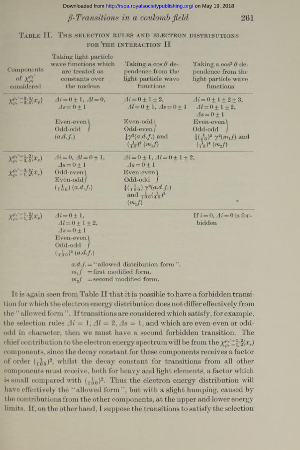
f3-Transitions in a coulomb field 261

T a ble II. T h e se l e c t io n r u l e s and e le c t r o n d ist r ib u t io n s

FOR THE INTERACTION II Taking light particle

Components

ofconsidered

wave functions which are trea ted as constants over

the nucleus

Taking a cos 6 dependence from the light particle wave

functions

Taking a cos2 6 dependence from the light particle wave

functions

XPp: ~ l \ \ ( x r A i - 0 ± 1, 0,d s = 0 ± 1

Even-even^ Odd-odd / (a.d.f.)

A i = 0 + 1 + 2,A l= 0 + 1, d s = 0 ± 1

Even-odd \Odd-even /

\ y 2(a.d.f.) and (to)2 (mi/)

A i - 0 + 1 ± 2 ± 3,Al = 0 ± 1 ± 2,

d s = 0 ± 1 Even-even)Ôdd-odd /K to)2 Y2(m iand(tV)4 (W2 /)

x pP:= l: l M

x pP:= l ; i W

A i — 0, A l — 0 + 1, d s = 0 ± 1

Odd-even)Even-odd J(ttto) ia -d.f.)

A i = 0 ± 1, Al = 0 ± 1 ± 2 , As = 0 + 1

Even-even)Odd-odd /t(tAo) y 2(a.d.f.)

and t ^ o(to)2( m j )

x% '= l;l(x r) A i — 0 + 1,ZlZ = 0 + 1 + 2,

I f i = 0, A i = 0 is forbidden

ds = 0± 1 Even-even)Odd-odd /(xiro)2 (a-d.f.)

a.d.f. = “ allowed distribution fo rm ” . m hf — first modified form. m2f = second modified form.

I t is again seen from Table II that it is possible to have a forbidden transition for which the electron energy distribution does not differ effectively from the “ allowed form ” . If transitions are considered which satisfy, for example, the selection rules Ai — 1, Al = 2, As = 1, and which are even-even or odd-odd in character, then we must have a second forbidden transition. The chief contribution to the electron energy spectrum will be from the components, since the decay constant for these components receives a factor of order (yô)2, whilst the decay constant for transitions from all other components must receive, both for heavy and light elements, a factor which is small compared with (yô)2- Thus the electron energy distribution will have effectively the “ allowed form ”, but with a slight humping, caused by the contributions from the other components, at the upper and lower energy limits. If, on the other hand, I suppose the transitions to satisfy the selection



262 F. Hoyle

rules Ai = 3, Al = 2, As = 1, and to have an even-even or odd-odd character, then it is seen that the corresponding electron spectrum will differ widely from the “ allowed form”.

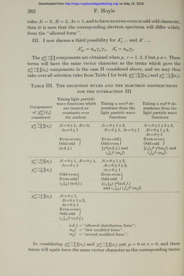
III. I now discuss a third possibility for J." ... and A'

jiv /uYv ’ m T r

The Xpr=l’,t components are obtained when/i, = 1, 2, 3 but Theseterms will have the same vector character as the terms which gave the XpPr=3’i(xr) components in the case II considered above, and we may thus take over all selection rules from Table I for both an(l

T a ble III. T h e se l e c t io n r u l e s a n d t h e e l e c t r o n d ist r ib u t io n s

EOR THE INTERACTION III Taking light particle

Componentsof x % Mconsidered

wave functions which are trea ted as constants over

the nucleus

Taking a cos 6 dependence from the light particle wave

functions

Taking a cos2 6 dependence from the light particle wave

functions

Ai = 0 ± 1, A l - 0, A i = 0 ± 1 ± 2 , A i= 0 ± 1 ± 2 ± 3,As = 0 + 1 A l= 0 ± 1, d s = 0 + 1 Al = 0 ± 1 ± 2,

d s = 0 ± 1Even-even) Even-odd) Even-even)Odd-odd / Odd-even / Odd-odd j{a.d.f.) \ y 2(a.d.f.) and

(to)2 (m J )F A ) 2 r 2(wi / ) and

(to)4 (m 2/)

x pPrr = l : iM

x pP:= l:l(x r)

A i= 0 ± 1, 0 ± 1,As = 0 ± 1

Odd-even)E ven-odd/(xifo) («-d./.)

A i = 0 + 1 + 2,A l— 0 + 1 + 2,

d s = 0 ± 1 Even-even)Odd-odd J Kxxx) Y2{a A .f.) and (t^ o) (to)2 (mif)

Aft-};! (xr) Ai=z°±1’Al — 0 ± 1 ± 2,ds = 0± 1

Even-even)Odd-odd J(xô)2 {a-d.f.)* a.d.f. = “ allowed distribution form ’’.

W j/ = “ first modified fo rm ” .m 2 f = “ second modified fo rm ” .

In considering Xpr-\’£ ixr) ancl X%=\\\{xr) put /£ = 0 or r = 0, and these terms will again have the same vector character as the corresponding terms



P-Transitions in a coulomb field 263

in the K.-U. case. Therefore the K.-U. selection rules for the components Xprr =i’,2(xr) and Xprr =l’,l(xr) may be taken over, and the table for this choice of A "..., A 'is obtained immediately from our two previous tables.

IV. Lastly, we may have

■Ajiv ^ 7^7 , 75, A v 5"

The Xprr=l’X(xr)and XPp[=\\\(xr) components are given by either = 0 orv = 0, and the same vector character for these components is obtained as in case II. Therefore the appropriate selection rules may be taken over from Table II.

To obtain the XPr =i\\(xr) and Xprr =s’,l(xr)components I must have / , v both different from zero, and once more this gives the same vector character as in the K.-U. case. Thus the table for this form of A"..., A... will be exactly of the same form as Table III.

In the above discussion of the possibilities for have neglectedall components of the wave functions T which have any spin co-ordinateexcept prwith the values 1, 2, where is the spin co-ordinate of the heavy particle making the transition. This means that the whole change of momentum comes from the transition particle. In the same approximation I must, however, consider the case in which the spin co-ordinate wdiich takes the values 1, 2 is not the spin co-ordinate of the transition particle. The only components of Xpfifixr) .which occur in this case are those for which pr — 3, 4, p'r — 3, 4, but we remember that is the sum of products ofthe components of the wave functions 0 , W where these are summations over all spin co-ordinates other than pr,p'r, and integrations over all space co-ordinates other than xr. The summations will now all be over the values 3, 4 with the exception of the particular spin co-ordinate to which all of the values 1, 2, 3, 4 are allowed, and this special summation will be of exactly the same type as the spin summation considered above for the K.-U. termwith p = 0 in the interaction A"fi__ Thus the various components in thissummation will contribute the selection rules given in the first and third rows of the first column of Table I (there being no selection rules similar to the second row, since no suitable components arise in the summation, and none similar to the second and third columns, since these are due to the properties of the light particle wave functions). I t is then seen that the total selection rules for the transition will depend upon the properties of this special summation, and it will depend also upon the summations over the spin co-ordinates of the transition particles, that is, over pr, 3, 4. There



264 F. Hoyle

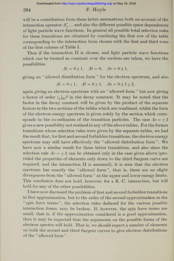
will be a contribution from these latter summations both on account of the interaction operator and also the different possible space dependences of light particle wave functions. In general all possible total selection rules for these transitions are obtained by combining the first row of the table corresponding to the interaction form chosen with the first and third rows of the first column of Table I.

Thus if the interaction II is chosen, and light particle wave functions which can be treated as constant over the nucleus are taken, we have the possibilities

Ai = 0+ 1, Al = 0, As = 0 ± 1,

giving an “ allowed distribution form” for the electron spectrum, and also Ai = 0± 1, A l= 0±1, 0±1 ±2 ,

again giving an electron spectrum with an “ allowed form” but now giving a factor of order (xw)2 in the decay constant. I t may be noted that the factor in the decay constant will be given by the product of the separate factors in the two sections of the tables which are combined, whilst the form of the electron energy spectrum is given solely by the section which corresponds to the co-ordinates of the transition particles. The case 2gives a new possibility not realized in any of the above tables. For the former transitions whose selection rules were given by the separate tables, we had the result that, for first and second forbidden transitions, the electron energy spectrum may still have effectively the “ allowed distribution form”. We have now a similar result for these latter transitions, and also since the selection rule As = ±2 can be obtained only in the case given above (provided the properties of elements only down to the third Sargent curve are required, and the interaction II is assumed), it is seen that the electron spectrum has exactly the “ allowed form”, that is, there are no slight divergences from the “ allowed form ” at the upper and lower energy limits. This conclusion does not hold, however, for a K.-U. interaction, but will hold for any of the other possibilities.

I have now discussed the problem of first and second forbidden transitions in first approximation, but to the order of the second approximation in the “ spin force terms”, the selection rules deduced for the various possible interaction forms, may be broken. If, however, the spin force terms are small, that is, if the approximation considered is a good approximation, then it may be expected that the arguments on the possible forms of the electron spectra will hold. That is, we should expect a number of elements on both the second and third Sargent curves to give electron distributions of the “ allowed form”.




My warmest thanks are due to Professor Peierls, both for many suggestions upon this problem, and for all I have learned from him. I am also greatly indebted to the Goldsmiths Company for their financial assistance.

A p p e n d ix

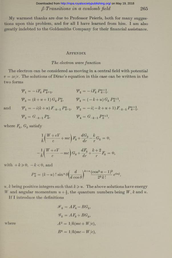
The electron wave function

The electron can be considered as moving in a central field with potential v = zejr. The solutions of Dirac’s equation in this case can be written in the two forms

= ~ iFk -Pji+i,

T 3 = (k 4- u + 1)

and T x = - i( + u) P£_l5

T 2 = - i F k P t th

P 4 = ( - k + u)Gk Pp-\

T 2 = - i i - k + u + l j F ^ ^

^ = gl*-i n +\

where Fk, Gk satisfy

1h

W + eV c + mc\Fk +dGf

dr = 0,

1 /W + eVh \

dFk 2 rfc_r drme I Gj, + — + • 0,

with + k 0, — <0, and

Pxk — ( k — u)\sinM0 d \ k+u(cos2u — I)*1d cos 6 2kk\

u, k being positive integers such that k The above solutions have energyW and angular momentum u + \, the quantum numbers being W, k and u.

If I introduce the definitions

3?k = AFk- B G k,

<Zk = AFk + BGk,

A 2 = l/h(mc + W/c),

B 2 — \jh(mc— W/c),

where



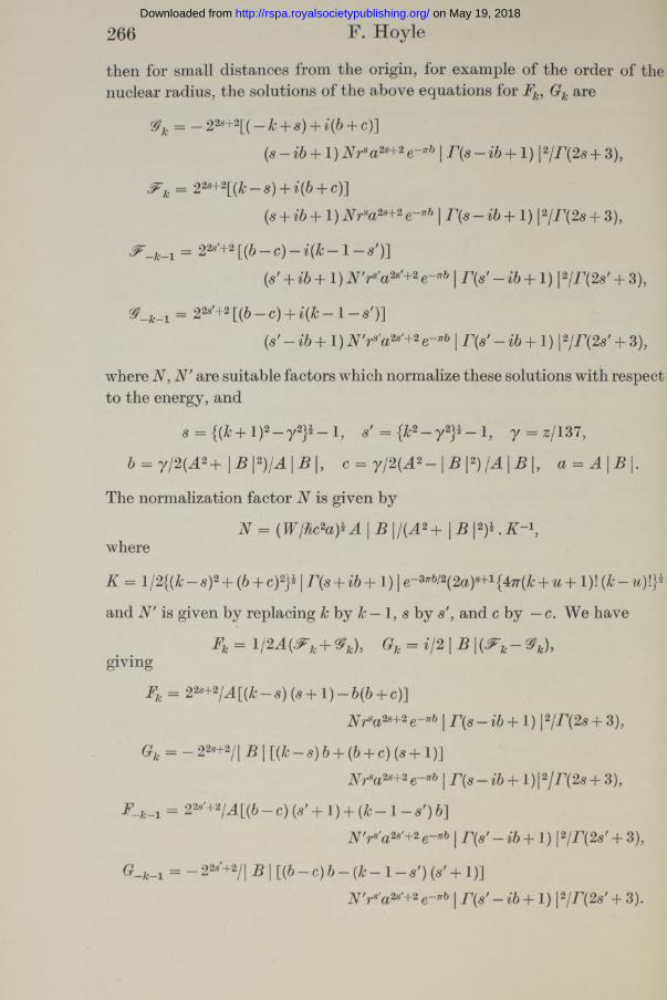
266 F. Hoyle

then for small distances from the origin, for example of the order of the nuclear radius, the solutions of the above equations for Gk are

@k = — 22s+2[( — k + s) + i(b + c)](s — ib+ 1) Nrsa2s+2 | 1) |2/F(2s + 3),

!Fk = 22s+2[{k — s) + i{b + c)](s + ib + 1) Nrsa2s+2 \ r(s + 1) 1 + 3),

= 22s'+2 [(6 — c) — i{k — 1 — «')]{s' +ib+l)N'rs’a2s'+2 \ r{s' + 1) 12/r (2s' + 3),

%_k_x = 22s'+2 [(6 - c ) + i ( k - l - s')]{s' —ib+ 1) N'rs'a2s'+2 e~vb \ F{s' + 1) 12/F(2 + 3),

where N, N' are suitable factors which normalize these solutions with respect to the energy, and

s = {(& + l)2 — y2}* — 1, s' = {k y2}* — 1, y = z/137,

b = y /2{A2+ \ B \2) /A \B \, c = y /2{A2- a = A \B \ .

The normalization factor N is given by

N = {W/kc2a ) iA \B \ /{ A 2+ \ B \ 2) i .K - \where

K = l /2{{k — s)2 + {b + c)2}*| r{s + ib+ 1) | e~37Tbl2{2a)s+1{4:7r{k + u+ 1)!

and N' is given by replacing kby k — 1, sby s', and c by — We have

Fk = 1/2 A (P k + s y , Gk = i/2 \B \ ( P k- 9 t ),giving

Fk = 22s+2IA[{k-s){s+l)-b{b + c)]Nrsa2s+2e~”b 1) 12/F(2s + 3),

Gk = - 22s+2/1 B| [(& - s) b + {b + c) {s + 1)]Nrsa2s+2e-I l) |2/ r ( 2s + 3),

F-k-! = 22s’+2IA[{b-c){s' + l) + { k - l - s ' ) b ]N'rs'a2s'+2e~”b | / > ' - + 1) 12/r{2s' + 3),

G-k-i = “ 22S'+2/1 B| [{b - c) b - {k - 1 - s') {s' 4- 1)]N'rs'a2s’+2 | r{s' 1) 12/r{2s' + 3).




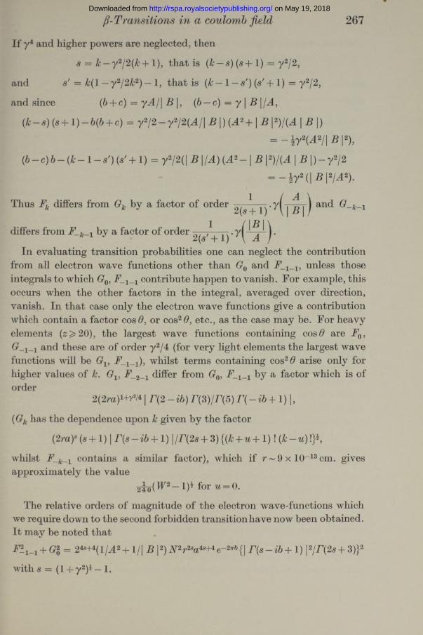
If y4 and higher powers are neglected, then

s = k — y 2j2{k+\), that is (Jc— (s+ 1) = y2/2,

and s' = k(l — y 2/2k2)—l, that is 1 — s') +1) = y2/2,

and since (b + c) = yA/\ B \, (b — c) = y \B \ /A ,

( k - s ) ( 8 + l ) - b ( b + c) = y2/2 - y 2/2(A/\ |) + 1 2)/(A | )

= - i r V 2/|B |2).( 6 - c ) 6 - ( fc-1 -« ') (*' +1) = y2/2(| I I I \ | ) - y 2/2

= - l r 2( | £ | 2/ ^ ) .

In evaluating transition probabilities one can neglect the contribution from all electron wave functions other than and unless thoseintegrals to which G0, jP_1_1 contribute happen to vanish. For example, this occurs when the other factors in the integral, averaged over direction, vanish. In that case only the electron wave functions give a contribution which contain a factor cos 6, or cos2 6, etc., as the case may be. For heavyelements ( z > 20), the largest wave functions containing cos 0 are F0,

and these are of order y2/4 (for very light elements the largest wave functions will be Gx, i rr_1__1), whilst terms containing cos2 6 arise only for higher values of Jc. Gv F_2_1 differ from G0, F_1_1 by a factor which is of order

( Gk has the dependence upon k given by the factor

(2 ra)s(s+ 1) | r (s — ib + 1) \/r(2s+ 3){(A; + ^ + 1)! ( !}*,

whilst F_fc_1 contains a similar factor), which if r ~ 9 x 10-13 cm. gives approximately the value

The relative orders of magnitude of the electron wave-functions which we require down to the second forbidden transition have now been obtained. It may be noted thatF- i-! + G2 = 24s+4(1/ 42+ 1/| B |2)2V2r2sa4s+4 e{| 1) |2/r(2s + 3)}2

with s = (I + y2)* — 1.

Thus Fkdiffers from Gk by a factor of order

differs from F

2(2ra)1+?2/4 | F (2 - ib) T (3 )/r(5 ) F( - + 1) | ,

2¥o(W2—!)* for 0.



268 F. Hoyle

Substituting for N 2 gives, apart from a numerical factor,

I P(s -f - ib+ l)/r(2s + 3) I2 l) i (Zrp/hfs,

since a = A/\ B| = ( W2/c2 — m2c2)* 1 /ft = (IF2 — 1)* = p/fo

and b — yW (

This is the factor mentioned above in the introductory remarks. +similarly contains this factor with the additional y2/4.

I t may be pointed out, finally, that if the wave functions for 0 and k = 1 are denoted by \Jr0 and i/r1} then for small r

but that 0 fo aîdr dr

Sum m ary

This paper attempts to give the selection rules, and the possible forms of the electron energy spectra, which correspond to elements on the first, second, and third Sargent curves, in the case of each of the possible forms of ^-interaction belonging to Hamiltonians that contain a derivative of only the neutrino wave function. This allows a choice of several possibilities for the interaction, among which is the form proposed by Konopinski and Uhlenbeck. The accurate solution of the problem would require a knowledge of the wave equation of a nucleus containing many particles. I assume that a non-relativistic Schrodinger equation can be formulated for the nucleus, in which the spin co-ordinate of each particle has two possible values (3, 4). The solutions of such equations for the initial and final nuclei will give a first type of forbidden transition. I t is further assumed that a relativistic equation can be constructed for the nuclei, in which the spin co-ordinate of each particle will now have four values (1, 2, 3, 4). From this point of view I regard the Schrodinger equations as given by neglecting, in the relativistic equations, all components of the wave function in which any spin co-ordinate is 1, 2. The Pauli reduction of the Dirac equation in the single-body problem is generalized to the assumption that a component of the wave function in which one spin co-ordinate is different from 3, 4 can be expressed to a suitable approximation, in terms of those components which occur in the Schrodinger equation, the connexion between these components being analogous to that given by Pauli in the one-body problem. This introduces small components of the wave fun ctions into the expression for the transition



[]-Transitions in a coulomb field 269

probability. These small components will have selection rules which are different from those for the large components, and transitions which were forbidden may now become “ allowed” for the small components (that is, the light particle wave functions may be treated as constants over the nucleus). I t is convenient to distinguish those components which are small in the spin variable of the transition particle, and those which are small in other variables. These two groups of small components will, in general, also have different selection rules. The result of comparing the selection rules for the three groups of components of the wave functions (the large components, and the two groups of small components), and of discussing the corresponding forms of the electron spectra, show that there may be elements on the second Sargent curve with either

(1) The “ allowed distribution form ’ ’ given by Konopi nski and Uhlenbeck, or possibly for light elements (nuclear charge^ 20):

(2) Electron distributions which differ from (1), and of types previously discussed (Hoyle 1937, p. 290, fig. 4, I, II),and that for elements on the third Sargent curve we have the possibilities:

(1) The ‘ ‘ allowed distribution form ’ ’ given by Konopinski and Uhlenbeck.(2) Effectively the distribution (1), but with a slight humping at the upper

and lower energy limits.(3) Distributions of the types previously discussed (Hoyle 1937, fig. 4, I,

II).(4) And for light elements (nuclear charge^20) distributions which

differ more widely from the “ allowed form” than (3), the shapes of these distributions being similar to (3), but of a more exaggerated form.

R e f e r e n c e s

Bethe, H. A. 1933 Handbuch der 24/1, 273- 560.Bethe, H. A. and Bacher, R. F . 1936 Rev. Mod. Phys. 8, 83- 229. Dirac, P. A. M. 1935 “ Principles of Q uantum Mechanics.”Ferm i, E. 1934 Z. Phys. 88, 161—77.Fierz, M. 1937 Helv. phys. Acta, 3 .Hoyle, F. 1937 Proc. Camb. Phil. Soc. 33, 277- 92.Hulme, H . R. 1931 Proc. Roy. Soc. A, 133, 381—406.Konopinski, E. J . and Uhlenbeck, G. E . 1935 Phys. Rev. 48, 7- 12. Nordheim, L. W. and Yost, F. L. 1937 Phys. Rev. 51, 943- 7.



Documents

The spectrum of thallium chloride 249 - Royal Societyrspa.royalsocietypublishing.org/content/royprsa/166/925/249.full.pdf · (xrp){A'...)pp,rJf{xrp’)^dT1...dTr