Embed Size (px)
Citation preview
U.S. Department of the InteriorU.S. Geological Survey
The South Florida Ecosystem Portfolio Model— A Map-Based Multicriteria Ecological, Economic, and Community Land-Use Planning Tool
Scientific Investigations Report 2009-5181

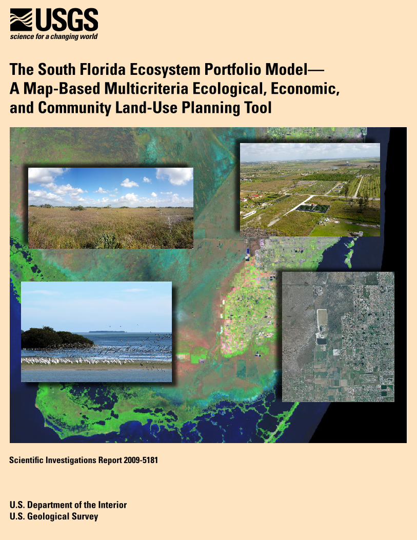
COVER. Landsat 7 image of South Florida (Bands 5, 4, and 3, collected between December 2003 and April 2004) (background). Insets are photos of Everglades National Park and a nearby agricultural area (photos courtesy of William Perry, Everglades National Park), as well as an orthoimage that shows the intersection of natural areas with agriculture and development land-uses near Bird Drive Basin in Miami-Dade County in 2006 (1.0 foot pixel-resolution color orthoimage obtained from the EROS Data Center, U.S. Geological Survey).
The South Florida Ecosystem Portfolio Model— A Map-Based Multicriteria Ecological, Economic, and Community Land-Use Planning Tool
By William B. Labiosa, Richard Bernknopf, Paul Hearn, Dianna Hogan, David Strong, Leonard Pearlstine, Amy M. Mathie, Anne M. Wein, Kevin Gillen, and Susan Wachter
Scientific Investigations Report 2009-5181
U.S. Department of the InteriorU.S. Geological Survey
U.S. Department of the InteriorKEN SALAZAR, Secretary
U.S. Geological SurveySuzette M. Kimball, Acting Director
U.S. Geological Survey, Reston, Virginia: 2009
This report and any updates to it are available online at:http://pubs.usgs.gov/sir/2009/5181/
For more information on the USGS—the Federal source for science about the Earth,its natural and living resources, natural hazards, and the environment:World Wide Web: http://www.usgs.gov/Telephone: 1-888-ASK-USGS
Any use of trade, product, or firm names in this publication is for descriptive purposes only and does not imply endorsement by the U.S. Government.
Although this report is in the public domain, it may contain copyrighted materials that are noted in the text. Permissionto reproduce those items must be secured from the individual copyright owners.
Suggested citation:Labiosa, W.B., Bernknopf, R., Hearn, P., Hogan, D., Strong, D., Pearlstine, L., Mathie, A.M., Wein, A.M., Gillen, K., and Wachter, S., 2009, The South Florida ecosystem portfolio model—A map-based multicriteria ecological, economic, and community land-use planning tool: U.S. Geological Survey Scientific Investigations Report 2009-5181, 41 p.
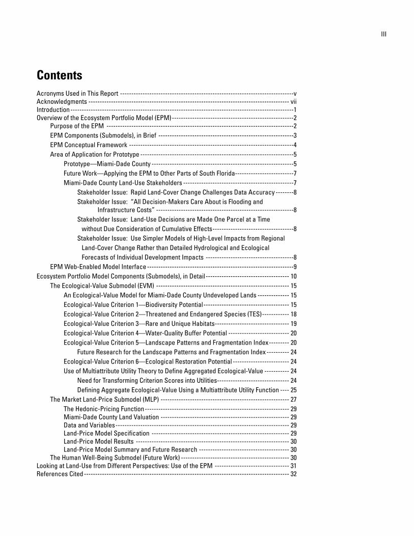
ContentsAcronyms Used in This Report -----------------------------------------------------------------------------vAcknowledgments ----------------------------------------------------------------------------------------- viiIntroduction ---------------------------------------------------------------------------------------------------1Overview of the Ecosystem Portfolio Model (EPM) ------------------------------------------------------2
Purpose of the EPM -----------------------------------------------------------------------------------2EPM Components (Submodels), in Brief ------------------------------------------------------------3EPM Conceptual Framework -------------------------------------------------------------------------4Area of Application for Prototype --------------------------------------------------------------------5
Prototype—Miami-Dade County ---------------------------------------------------------------5Future Work—Applying the EPM to Other Parts of South Florida --------------------------7Miami-Dade County Land-Use Stakeholders -------------------------------------------------7
Stakeholder Issue: Rapid Land-Cover Change Challenges Data Accuracy --------8Stakeholder Issue: “All Decision-Makers Care About is Flooding and
Infrastructure Costs” -------------------------------------------------------------8Stakeholder Issue: Land-Use Decisions are Made One Parcel at a Time without Due Consideration of Cumulative Effects ------------------------------------8Stakeholder Issue: Use Simpler Models of High-Level Impacts from Regional Land-Cover Change Rather than Detailed Hydrological and Ecological Forecasts of Individual Development Impacts ---------------------------------------8
EPM Web-Enabled Model Interface -----------------------------------------------------------------9Ecosystem Portfolio Model Components (Submodels), in Detail ------------------------------------- 10
The Ecological-Value Submodel (EVM) ----------------------------------------------------------- 15An Ecological-Value Model for Miami-Dade County Undeveloped Lands -------------- 15Ecological-Value Criterion 1—Biodiversity Potential -------------------------------------- 15Ecological-Value Criterion 2—Threatened and Endangered Species (TES) ------------ 18Ecological-Value Criterion 3—Rare and Unique Habitats --------------------------------- 19Ecological-Value Criterion 4—Water-Quality Buffer Potential --------------------------- 20Ecological-Value Criterion 5—Landscape Patterns and Fragmentation Index --------- 20
Future Research for the Landscape Patterns and Fragmentation Index ---------- 24Ecological-Value Criterion 6—Ecological Restoration Potential ------------------------- 24Use of Multiattribute Utility Theory to Define Aggregated Ecological-Value ----------- 24
Need for Transforming Criterion Scores into Utilities -------------------------------- 24Defining Aggregate Ecological-Value Using a Multiattribute Utility Function ---- 25
The Market Land-Price Submodel (MLP) --------------------------------------------------------- 27The Hedonic-Pricing Function ---------------------------------------------------------------- 29Miami-Dade County Land Valuation --------------------------------------------------------- 29Data and Variables ----------------------------------------------------------------------------- 29Land-Price Model Specification ------------------------------------------------------------- 29Land-Price Model Results -------------------------------------------------------------------- 30Land-Price Model Summary and Future Research ---------------------------------------- 30
The Human Well-Being Submodel (Future Work) ------------------------------------------------ 30Looking at Land-Use from Different Perspectives: Use of the EPM --------------------------------- 31References Cited ------------------------------------------------------------------------------------------- 32
III
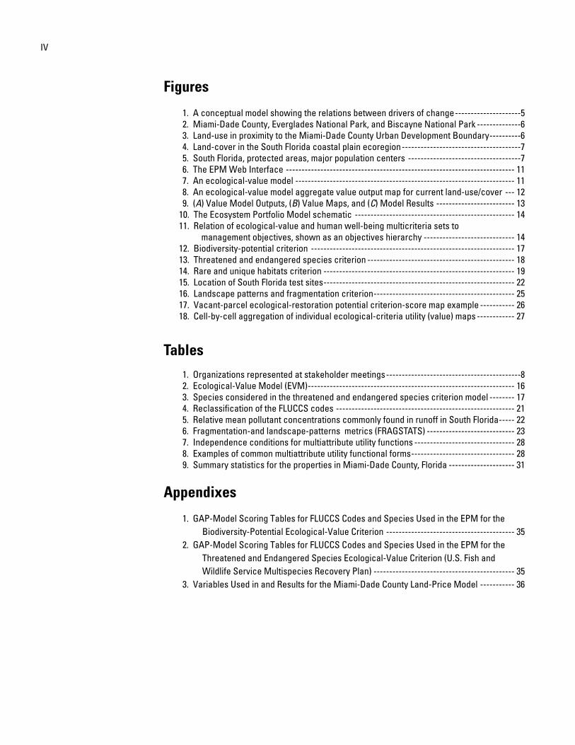
Figures
1. A conceptual model showing the relations between drivers of change ---------------------5 2. Miami-Dade County, Everglades National Park, and Biscayne National Park --------------6 3. Land-use in proximity to the Miami-Dade County Urban Development Boundary ----------6 4. Land-cover in the South Florida coastal plain ecoregion --------------------------------------7 5. South Florida, protected areas, major population centers ------------------------------------7 6. The EPM Web Interface ------------------------------------------------------------------------- 11 7. An ecological-value model ---------------------------------------------------------------------- 11 8. An ecological-value model aggregate value output map for current land-use/cover --- 12 9. (A) Value Model Outputs, (B) Value Maps, and (C) Model Results ------------------------- 13 10. The Ecosystem Portfolio Model schematic --------------------------------------------------- 14 11. Relation of ecological-value and human well-being multicriteria sets to management objectives, shown as an objectives hierarchy ----------------------------- 14 12. Biodiversity-potential criterion ----------------------------------------------------------------- 17 13. Threatened and endangered species criterion ----------------------------------------------- 18 14. Rare and unique habitats criterion ------------------------------------------------------------- 19 15. Location of South Florida test sites ------------------------------------------------------------- 22 16. Landscape patterns and fragmentation criterion --------------------------------------------- 25 17. Vacant-parcel ecological-restoration potential criterion-score map example ----------- 26 18. Cell-by-cell aggregation of individual ecological-criteria utility (value) maps ------------ 27
Tables 1. Organizations represented at stakeholder meetings -------------------------------------------8 2. Ecological-Value Model (EVM) ------------------------------------------------------------------ 16 3. Species considered in the threatened and endangered species criterion model -------- 17 4. Reclassification of the FLUCCS codes --------------------------------------------------------- 21 5. Relative mean pollutant concentrations commonly found in runoff in South Florida ----- 22 6. Fragmentation-and landscape-patterns metrics (FRAGSTATS) ---------------------------- 23 7. Independence conditions for multiattribute utility functions -------------------------------- 28 8. Examples of common multiattribute utility functional forms --------------------------------- 28 9. Summary statistics for the properties in Miami-Dade County, Florida --------------------- 31
Appendixes
1. GAP-Model Scoring Tables for FLUCCS Codes and Species Used in the EPM for the Biodiversity-Potential Ecological-Value Criterion ----------------------------------------- 352. GAP-Model Scoring Tables for FLUCCS Codes and Species Used in the EPM for the Threatened and Endangered Species Ecological-Value Criterion (U.S. Fish and Wildlife Service Multispecies Recovery Plan) --------------------------------------------- 353. Variables Used in and Results for the Miami-Dade County Land-Price Model ----------- 36
IV
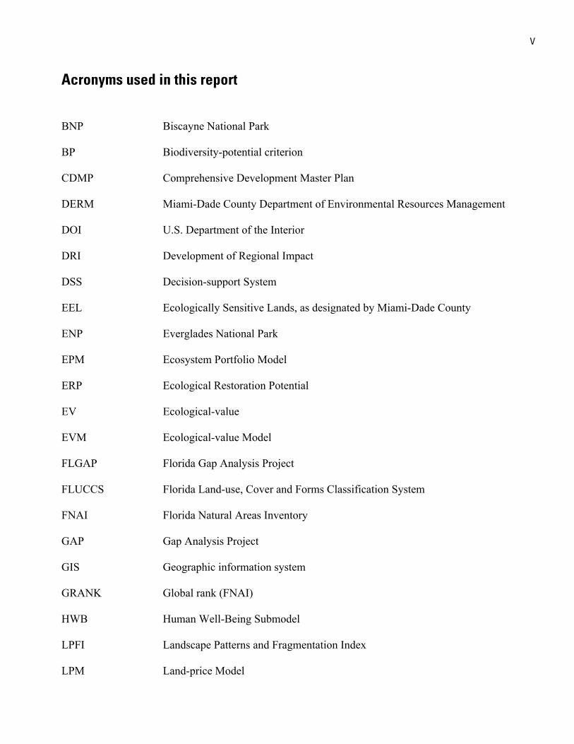
Acronyms used in this report
BNP Biscayne National Park
BP Biodiversity-potential criterion
CDMP Comprehensive Development Master Plan
DERM Miami-Dade County Department of Environmental Resources Management
DOI U.S. Department of the Interior
DRI Development of Regional Impact
DSS Decision-support System
EEL Ecologically Sensitive Lands, as designated by Miami-Dade County
ENP Everglades National Park
EPM Ecosystem Portfolio Model
ERP Ecological Restoration Potential
EV Ecological-value
EVM Ecological-value Model
FLGAP Florida Gap Analysis Project
FLUCCS Florida Land-use, Cover and Forms Classification System
FNAI Florida Natural Areas Inventory
GAP Gap Analysis Project
GIS Geographic information system
GRANK Global rank (FNAI)
HWB Human Well-Being Submodel
LPFI Landscape Patterns and Fragmentation Index
LPM Land-price Model
V
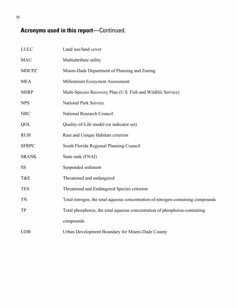
LULC Land use/land cover
MAU Multiattribute utility
MDCPZ Miami-Dade Department of Planning and Zoning
MEA Millennium Ecosystem Assessment
MSRP Multi-Species Recovery Plan (U.S. Fish and Wildlife Service)
NPS National Park Service
NRC National Research Council
QOL Quality-of-Life model (or indicator set)
RUH Rare and Unique Habitats criterion
SFRPC South Florida Regional Planning Council
SRANK State rank (FNAI)
SS Suspended sediment
T&E Threatened and endangered
TES Threatened and Endangered Species criterion
TN Total nitrogen, the total aqueous concentration of nitrogen-containing compounds
TP Total phosphorus, the total aqueous concentration of phosphorus-containing
compounds
UDB Urban Development Boundary for Miami-Dade County
UEA Urban Expansion Area for Miami-Dade County
USGS U.S. Geological Survey
WQBP Water-quality Buffer Potential criterion
Acronyms used in this report—Continued.
VI
VII
Acknowledgments
The authors would like to acknowledge the many useful discussions with David Hallac, Linda
Friar, Betty Grizzle and Robert Johnson from Everglades National Park, Sarah Bellmund and Mark
Lewis from Biscayne National Park, Ronnie Best and the Priority Ecosystems Science Program
from the U.S. Geological Survey (USGS), Jonathan Smith and the Geographic Analysis and Moni-
toring Program from the USGS, Don DeAngelis and William Forney from the USGS, Subrata Basu
from the Miami-Dade County Department of Planning and Zoning, Frank Muzzotti from the Uni-
versity of Florida, Les Vilchek and Patrick Pitts from the U.S. Fish and Wildlife Service, and Gwen
Burzycki from the Miami-Dade County Department of Environmental Resources Management.
We would also like to acknowledge the significant roles played by David Hallac and Sarah Bell-
mund in choosing the ecological criteria used in the ecological-value model. Lastly, we would like
to acknowledge our newly formed collaboration with Hugh Gladwin from Florida International
University and Ann- Margaret Esnard from Florida Atlantic University supporting the creation and
implementation of a set of land-use-related human well-being metrics for Miami-Dade County.

This page intentionally left blank
1
Introduction
The South Florida Ecosystem Portfolio Model (EPM) prototype is a regional land-use planning Web tool that inte-grates ecological, economic, and social information and values of relevance to decision-makers and stakeholders. The EPM uses a multicriteria evaluation framework that builds on geographic information system-based (GIS) analysis and spatially-explicit models that characterize important ecological, economic, and societal endpoints and consequences that are sensitive to regional land-use/land-cover (LULC) change. The EPM uses both economics (monetized) and multiattribute util-ity (nonmonetized) approaches to valuing these endpoints and consequences. This hybrid approach represents a methodologi-cal middle ground between rigorous economic and ecological/ environmental scientific approaches. The EPM sacrifices some degree of economic- and ecological-forecasting precision to gain methodological transparency, spatial explicitness, and transferability, while maintaining credibility. After all, even small steps in the direction of including ecosystem services evaluation are an improvement over current land-use planning practice (Boyd and Wainger, 2003).
There are many participants involved in land-use decision-making in South Florida, including local, regional, State, and Federal agencies, developers, environmental groups, agricul-tural groups, and other stakeholders (South Florida Regional Planning Council, 2003, 2004). The EPM’s multicriteria evaluation framework is designed to cut across the objectives and knowledge bases of all of these participants. This approach places fundamental importance on social equity and stakeholder participation in land-use decision-making, but makes no attempt
to determine normative socially “optimal” land-use plans. The EPM is thus a map-based set of evaluation tools for planners and stakeholders to use in their deliberations of what is “best”, considering a balancing of disparate interests within a regional perspective. Although issues of regional ecological sustain-ability can be explored with the EPM (for example, changes in biodiversity potential and regional habitat fragmentation), it does not attempt to define or evaluate long-term ecological sustainability as such. Instead, the EPM is intended to provide transparent first-order indications of the direction of ecological, economic, and community change, not to make detailed predic-tions of ecological, economic, and social outcomes. In short, the EPM is an attempt to widen the perspectives of its users by inte-grating natural and social scientific information in a framework that recognizes the diversity of values at stake in South Florida land-use planning.
For terrestrial ecosystems, land-cover change is one of the most important direct drivers of changes in ecosystem services (Hassan and others, 2005). More specifically, the fragmenta-tion of habitat from expanding low-density development across landscapes appears to be a major driver of terrestrial species decline and the impairment of terrestrial ecosystem integrity, in some cases causing irreversible impairment from a land-use planning perspective (Brody, 2008; Peck, 1998). Many resource managers and land-use planners have come to realize that evalu-ating land-use conversions on a parcel-by-parcel basis leads to a fragmented and narrow view of the regional effects of natural land-cover loss to development (Marsh and Lallas, 1995). The EPM is an attempt to integrate important aspects of the coupled natural-system/human-system view from a regional planning perspective.
The EPM evaluates proposed land-use changes, both conversion and intensification, in terms of relevant ecological, economic, and social criteria that combine information about probable land-use outcomes, based on ecological and environ-mental models, as well as value judgments, as expressed in user-modifiable preference models. Based on on-going meet-ings and interviews with stakeholders and potential tool users,
The South Florida Ecosystem Portfolio Model— A Map-Based Multicriteria Ecological, Economic, and Community Land-Use Planning Tool
By William B. Labiosa1, Richard Bernknopf1, Paul Hearn2, Dianna Hogan2, David Strong2, Leonard Pearlstine3, Amy M. Mathie1, Anne M. Wein1, Kevin Gillen4, and Susan Wachter4
1 U.S. Geological Survey, Menlo Park, CA 94025. 2 U.S. Geological Survey, Reston, VA 20192.3 Everglades and Dry Tortugas National Parks, Homestesd, FL 33030.4 Wharton School, University of Pennsylvania, Philadelphia, PA 19104.
2 The South Florida Ecosystem Portfolio Model
we focus on three dimensions of LULC-related anthropocentric value (1) ecological-value (based on various ecological criteria), (2) market land-price, and (3) indicators of (human) community quality-of-life or human well-being. Each of these dimensions is implemented as a submodel of the EPM that generates “value maps” for a given land-use pattern, where the value map reflects changes in land attributes and patterns, as well as user prefer-ences (the exception is the land-price model, which reflects market prices outside of the influence of the individual user). These attributes are primarily related to land-use and land-cover, including changes in habitat potential and landscape fragmenta-tion, human perceived amenities, community character, flooding and hurricane evacuation risks, water-quality buffer potential, and ecological restoration potential, and other relevant criteria. Each of the submodels is discussed in detail in this report. Note that what is “good” from the perspective of one submodel (for example, increased habitat potential within the ecological-value model) may be “bad” from another (for example, increased travel time to shopping within the community quality-of-life model), so the resulting submodel scores can conflict for a given land-use pattern. Related to this, the EPM is designed to allow users to consider trade-offs between competing values, since the value maps (ecological-value, land-price, and community quality-of-life) can be broken down into underlying individual criteria values, as well as viewed as aggregated value maps.
The EPM is designed to be used by a variety of users for a variety of contexts. Examples of potential users and contexts include: 1) Federal, State, and local natural resource agency staff and managers that review development applications and land-use plans; 2) various stakeholders interested in evaluating development applications, comparing land-use plans, and evalu-ating land-use trends; 3) local and regional planning agency staff evaluating potential ecological impacts to protected public lands and private undeveloped lands; and 4) resource agency staff communicating with land-use decision-makers and other stakeholders about the potential effects of surrounding land-use change to their protected resources. The EPM Web interface allows such users to choose from a list of existing land-use plans, to upload their own land-use plans using a specified clas-sification system, and, through the Web interface, to interac-tively modify the land-use classifications of any cells or parcels within a loaded land-use plan.
There are other examples of GIS-based land-use planning tools (for example, CommunityViz™ (http://www.communityviz.com), CITYgreen (http://www.americanforests.org/productsandpubs/citygreen/; last accessed July 2, 2008), and Smart Places (www.ncseonline.org/NCSSF/DSS/Documents/NatureServe/SmartPlace.doc; last accessed July 2, 2008), ecosystem management tools (for example, Ecosystem-Based Management Tools Network at http://www.smartgrowthtools.org/ebmtools/index.php; last accessed July 2, 2008), and regional ecosystem services evaluation tools (for example, the Natural Capital Project InVEST toolbox at http://www.naturalcapitalproject.org/toolbox.html; last accessed July 30, 2009). However, these tools have a different focus and intended use. They are designed to be
general tools that must be customized with local data and infor-mation by users (or consultants) for application in a specific place and context. In contrast, the EPM is designed to be used as a place-specific set of Web-accessed tools implemented for a relatively small number of high priority ecosystems experienc-ing intense land-use change due to urbanization and sprawl. Also, the EPM is designed to enable a “strong sustainability view” of the regional impacts and tradeoffs inherent in land-use change. From this perspective, ecological, economic, and quality-of-life endpoints must be tracked separately, since a loss in natural capital is not assumed to be necessarily offset by a gain in other capital (Goodland and Daly, 1995). Decision-mak-ers may still choose to make this tradeoff, but the EPM makes the ecological-economic-community value tradeoffs explicit, without combining these categorically-distinct values.
The South Florida EPM is designed as a maintained public Web page (http://lcat.usgs.gov/sflorida/sflorida.html; user name is “sflorida” and the password is “alligator” ; last accessed July 30, 2009) that will be modified as new data is collected, models are improved, and new needs are identified. An important part of the customization is the creation of a self-contained and user-friendly Web interface that directly links inputted land-use patterns to models, where the models are chosen, created, and/or modified during an initial user/stakeholder analysis phase and post-prototype evaluation phase. Although the approach is transferable to any urban-natural interface, the South Florida EPM is customized to the issues and values at stake in South Florida. Plans to apply the EPM to Puget Sound in Washington and the San Santa Cruz Watershed in Arizona and Sonora, Mexico, are being developed.
Overview of the Ecosystem Portfolio Model (EPM)Purpose of the EPM
The EPM is designed as a flexible and user-friendly Web tool for addressing a complex set of land-use planning needs for a variety of potential users, including stakeholders, land-use planners, and researchers. These needs include (1) link-ing land-use changes to changes in relevant ecological-values and biophysical endpoints, (2) linking land-use change and its consequences to changes in economic values, and (3) linking land-use changes to changes in indicators of human well-being. Quantifying these linkages rigorously is notoriously difficult, both from a practical and theoretical point-of-view (Banzhaf and Boyd, 2005; Figge, 2004; Goodstein, 2002; Millennium Ecosystem Assessment, 2003; National Research Council, 1994; National Research Council, 2005). The EPM frames land-use decision-making using performance criteria and management objectives at the regional scale, making use of GIS analysis and simple appropriate models, recognizing the poten-tial for conflicting goals and value trade-offs for a given user, as
3
well as divergent preferences between different users. Although the EPM itself does not impose any particular decision-delib-eration process, it is designed to be flexible and transparent enough to be used in public deliberation processes that foster consensus-building and stakeholder equity, which refers to the fair treatment of competing social groups involved in land-use decision-making (Wilson and Howarth, 2002). The design of the EPM reflects workshops and meetings held with potential users and local land-use stakeholders so that these linkages are made at their desired level of sophistication, where the linkages are represented using accepted concepts and trusted models and approaches, while allowing enough flexibility for different users to impose their own prioritizations of criteria and management objectives.
For a given potential land-use pattern, the EPM is designed to evaluate (1) ecological criteria scores indicative of the land-scape’s ability to provide ecosystem goods and services at the local and regional scale, (2) the ecological restoration potential for individual parcels, (3) predicted land-prices, a surrogate for future development pressure, and (4) indicators of community quality-of-life or human well-being, including amenities, risks, and livability. Note that the EPM is a work in progress and that the submodels are still being refined. Also note that the com-munity quality-of-life component is the last submodel to be addressed and is currently in the design phase.We describe each of these dimensions of human-ascribed value in the sections that follow.
Although the EPM is designed for real-world use, it is also a research project. From the perspective of the U.S. Department of the Interior (DOI) Science Plan for South Florida (http://sofia.usgs.gov/publications/reports/doi-science-plan/; last accessed July 31, 2009), the EPM addresses aspects of the fol-lowing questions and needs:
• What are the socioeconomic consequences of development and preservation/restoration decisions associated with criti-cal components of the South Florida ecosystem?
• Are there ways to increase the sustainable compatibility of the built environment with natural-system needs of national parks and refuges, especially, with regards to water-related challenges?
• Conduct studies to estimate the economic value of key environmental and ecological resources affected by devel-opment and preservation/restoration decisions;
• Aggregate and quantify the large uncertainties associated with these decisions; and
• Develop a GIS-based decision framework in a decision-support system (DSS) that will provide land managers and local officials with a clearer idea of the economic conse-quences of various courses of action.
EPM Components (Submodels), in Brief
The ecological-value model (EVM), one of the three principal components (or submodels) of the EPM, compares
local and regional land-use/land-cover (LULC) patterns in terms of ecological criteria related to biodiversity, habitat patterns and fragmentation, habitat rarity and diversity, the ability to buffer water-quality in run-off to Biscayne Bay, and the potential for ecological restoration. The comparison is done in terms of model-based scores for each criterion, reflecting potential ecological and environmental responses to LULC changes and important consequences of those changes. The criteria evalu-ation model scores are transformed into multiattribute utilities to reflect user preferences over the scores for each criterion through the use of user-assigned utility parameters and, in some cases, subcriterion weights. For example, a unit increase for low scores may be significantly more important to the user than a unit increase for high scores. By transforming the model scores into user-defined utilities, changing marginal utility may be captured. The relative importance between the different criteria can also be adjusted by the user through user-assigned weights for each criterion and subcriterion. As described in detail in the Ecosystem Portfolio Model Components section, multiat-tribute utility approaches are used to allow direct comparison of criteria scores and to allow rigorous aggregation of individual criteria scores into an aggregate ecological-value score. The aggregate ecological-value depends on preferences elicited from the individual user, so the user’s ecological-value map reflects both objective ecological information, as well as subjective user information. In other words, an ecological-value map represents the individual user’s values. To generate an ecological-value map that represents the consensus values of stakeholders and decision-makers, criteria weights and utility parameters must be agreed upon by all decision participants. The EVM criteria were chosen in collaboration with scientists and managers at the Everglades National Park, Biscayne National Park and U.S. Fish and Wildlife Service, and are undergoing a peer review process, as described in the final section of this report. Resource manag-ers and staff scientists in Federal, State, and local agencies are interested in understanding the ecological and environmental effects of land-use and land-use patterns in lands near important natural resources because they are stakeholders in local and regional land-use decisions. These agencies take part in land-use planning in a variety of ways, and the EVM is designed to be a useful land-use evaluation tool, both from an analytical and a communications perspective.
The market land-price submodel (MLP) evaluates land-price as a function of LULC patterns and other predictor variables. The MLP is based on hedonic-pricing functions, which describe each land parcel’s price in terms of its particular characteristics (for example, parcel size and zoning), as well as amenities and disamenities related to location. Amenity variables (variables that tend to increase price) include dis-tances to central business districts, other built amenities, and environmental amenities, such as natural areas, open space, and recreational areas. Disamenity variables (variables that tend to decrease price) include distances to nonnavigable canals, as well as restrictions on land-use and development. Of course, the states of these amenity and disamenity variables may be related
Overview of the Ecosystem Portfolio Model (EPM)
4 The South Florida Ecosystem Portfolio Model
to the states of the LULC variables that drive the EVM. The MLP allows the user to explore the effects of proposed land-use changes (development, restored natural uses, and other factors) on surrounding parcel prices, which has implications for future development pressure for those parcels. These predicted price changes and changes in development pressure are an example of an economic externality associated with land-use planning. An externality is a consequence of a market transaction affecting parties or entities not directly involved in the transaction. The transaction price thus does not reflect these external conse-quences, thus resulting in a misallocation of land uses.
The human well-being (HWB) submodel uses data and models to evaluate a set of human well-being indicators (data-based) and metrics (model-based) of interest to the public, land-use planners, and stakeholders. Possible indicators include flood risk, hurricane evacuation times, and green space extent and placement, and aggregate indices of aspects of community well-being. The indicators and indices will be selected during an initial user/stakeholder meeting process and will be refined based on feedback from a post-prototype evaluation. An indica-tor or metric, in this context, is a single measure of the condition of one aspect of community quality-of-life, chosen to indicate the status or quality of that aspect. An index is a synthesis of several indicators and is designed to summarize several aspects of community quality-of-life or human well-being. Indicators and metrics can be organized hierarchically, with sub-sets being synthesized into sub-indices, which are then synthesized into an over-all index. The EPM is designed to allow access to individ-ual indicators, as well as indices based on these indicators. User preferences for individual indicators and metrics and aggregated indicators, metrics, and indices will be modeled using multiat-tribute utility approaches. The user will have the ability to assign and modify utility parameters through the EPM Web interface.
EPM Conceptual Framework
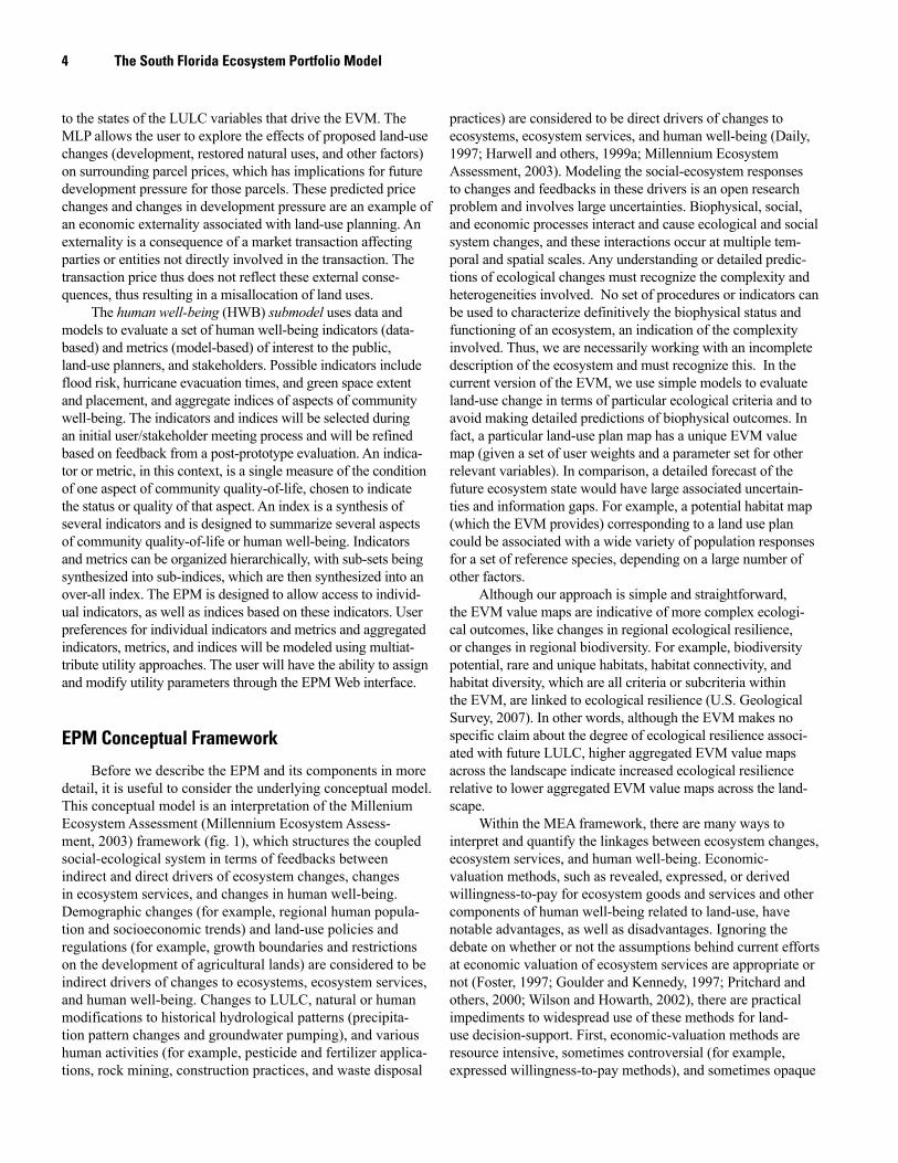
Before we describe the EPM and its components in more detail, it is useful to consider the underlying conceptual model. This conceptual model is an interpretation of the Millenium Ecosystem Assessment (Millennium Ecosystem Assess-ment, 2003) framework (fig. 1), which structures the coupled social-ecological system in terms of feedbacks between indirect and direct drivers of ecosystem changes, changes in ecosystem services, and changes in human well-being. Demographic changes (for example, regional human popula-tion and socioeconomic trends) and land-use policies and regulations (for example, growth boundaries and restrictions on the development of agricultural lands) are considered to be indirect drivers of changes to ecosystems, ecosystem services, and human well-being. Changes to LULC, natural or human modifications to historical hydrological patterns (precipita-tion pattern changes and groundwater pumping), and various human activities (for example, pesticide and fertilizer applica-tions, rock mining, construction practices, and waste disposal
practices) are considered to be direct drivers of changes to ecosystems, ecosystem services, and human well-being (Daily, 1997; Harwell and others, 1999a; Millennium Ecosystem Assessment, 2003). Modeling the social-ecosystem responses to changes and feedbacks in these drivers is an open research problem and involves large uncertainties. Biophysical, social, and economic processes interact and cause ecological and social system changes, and these interactions occur at multiple tem-poral and spatial scales. Any understanding or detailed predic-tions of ecological changes must recognize the complexity and heterogeneities involved. No set of procedures or indicators can be used to characterize definitively the biophysical status and functioning of an ecosystem, an indication of the complexity involved. Thus, we are necessarily working with an incomplete description of the ecosystem and must recognize this. In the current version of the EVM, we use simple models to evaluate land-use change in terms of particular ecological criteria and to avoid making detailed predictions of biophysical outcomes. In fact, a particular land-use plan map has a unique EVM value map (given a set of user weights and a parameter set for other relevant variables). In comparison, a detailed forecast of the future ecosystem state would have large associated uncertain-ties and information gaps. For example, a potential habitat map (which the EVM provides) corresponding to a land use plan could be associated with a wide variety of population responses for a set of reference species, depending on a large number of other factors.
Although our approach is simple and straightforward, the EVM value maps are indicative of more complex ecologi-cal outcomes, like changes in regional ecological resilience, or changes in regional biodiversity. For example, biodiversity potential, rare and unique habitats, habitat connectivity, and habitat diversity, which are all criteria or subcriteria within the EVM, are linked to ecological resilience (U.S. Geological Survey, 2007). In other words, although the EVM makes no specific claim about the degree of ecological resilience associ-ated with future LULC, higher aggregated EVM value maps across the landscape indicate increased ecological resilience relative to lower aggregated EVM value maps across the land-scape.
Within the MEA framework, there are many ways to interpret and quantify the linkages between ecosystem changes, ecosystem services, and human well-being. Economic-valuation methods, such as revealed, expressed, or derived willingness-to-pay for ecosystem goods and services and other components of human well-being related to land-use, have notable advantages, as well as disadvantages. Ignoring the debate on whether or not the assumptions behind current efforts at economic valuation of ecosystem services are appropriate or not (Foster, 1997; Goulder and Kennedy, 1997; Pritchard and others, 2000; Wilson and Howarth, 2002), there are practical impediments to widespread use of these methods for land-use decision-support. First, economic-valuation methods are resource intensive, sometimes controversial (for example, expressed willingness-to-pay methods), and sometimes opaque
5
to decision-makers and stakeholders (Boyd and Wainger, 2003). On the other hand, economic-valuation methods are the most defensible approaches, if one accepts the assumptions on which they are based (Pritchard and others, 2000). Some ecol-ogists, economists, and social scientists argue that economic valuation approaches work well within a system of static and well-behaved goods and services, but that ecosystem change and longer-term ecosystem management do not meet these criteria. Many other criticisms and defenses can be found in the literature (Costanza and others, 1997; Costanza and Folke, 1997; Foster, 1997; Heal, 2000; National Research Council, 1994; Pritchard and others, 2000; Wilson and Howarth, 2002).
The EVM takes a multiattribute utility approach to valu-ation of ecosystem services with no attempt at monetization. Although the economic component of the EPM does track the predicted monetized changes in market price of land parcels due to changes in land-use and other associated changes, this is only one component of the many values at stake. The use of a mul-ticriteria framework represents a pragmatic trade-off between economic rigor and assessment burden. Multicriteria weights and multiattribute utility functions can be assessed directly from users and debated within a participatory decision-making pro-cess. Sensitivity analysis on weights and utility parameters can
help address questions about the degree to which user prefer-ences affect value maps.
Direct-assessment methods within a participatory decision-making process may be more appropriate for some decision-making situations, including land-use decisions (Wilson and Howarth, 2002). This is not to argue that economic valuation of ecosystem services is inappropriate for land-use decision-making but rather that we hope our chosen decision-support framework represents a practical and useful step in the direction of integrated ecological-economic analytical support for partici-patory land-use decision-support.
Area of Application for Prototype
Prototype—Miami-Dade County
Although we propose to extend the application of the EPM throughout areas of interest in South Florida, the focus for the prototype implementation is Miami-Dade County. Miami-Dade County includes highly urbanized areas, as well as low-density agricultural areas and protected natural areas outside of the
Overview of the Ecosystem Portfolio Model (EPM)
Figure 1. A conceptual model showing the relations between drivers of change, ecosystem services, and human well-being. Based on the Millennium Ecosystem Assessment Conceptual Model (MEA, 2003).
HUMAN WELL-BEING* Health and safety* Material well-being* Social well-being* Options for change
INDIRECT DRIVERS OF CHANGE* Demographic* Land-use policies* Water-management policies
DRIVERS OF CHANGE* Changes in land-use and land-cover* External inputs (fertilizers, pesticides)* Resource extraction (mining, water � � � � withdrawals)* Ecological restoration
ECOSYSTEM SERVICES BIODIVERSITY, ENVIRONMENT, AND CLIMATE* Provisioning (fishing, agriculture, water)* Regulating (flood control, clean water, � � storm protection)* Cultural (recreational, spiritual, aesthetic)* Supporting (primary production, wetland � � and soil maintenance)
Human and natural influences, human interventions possible
Natural influences, little human intervention possible
Processes and linkages operate over multipletemporal and spatial scales
6 The South Florida Ecosystem Portfolio Model
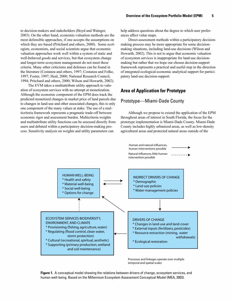
Urban Development Boundary (UDB) that currently serve as “buffer lands” between human development and Everglades and Biscayne National Parks (figs. 2 and 3). These buffer lands pro-vide vital hydrologic and ecological links between the national parks but are links which can be impacted by human develop-ment. The vacant and agricultural lands outside of the UDB face development pressure (Grunwald, 2006; Rabin and Pinzur, 2008; Solecki and others, 1999; Zwick and Carr, 2006), and this pressure is expected to increase as the Miami-Dade County human population increases from 2.4 million to around 3 mil-lion people by 2020 (26 percent increase; (Miami-Dade County Department of Planning & Zoning, 2008).
Miami-Dade County is unique in that it is the only major metropolitan area in the United States that borders two national parks, Everglades National Park and Biscayne National Park (http://www.miamidade.gov; last accessed July 31, 2009). The Everglades, which include a wide variety of environments and wildlife, are themselves unique geographically and ecologically (Davis and others, 1994; National Research Council, 2007). Biscayne Bay, adjacent to South Miami and within sight of downtown Miami, has four primary ecosystem types (1) man-grove forest along the mainland shore, (2) the southern bay, (3) the northernmost Florida Key islands, and (4) parts of the third-largest coral reef in the world. South Florida’s national parks, wildlife refuges, and other protected areas have a variety of mandates to protect local and regional ecological and environ-mental assets within their borders. Protected public lands com-prise approximately 70 percent of Miami-Dade County’s 1.3 million acres, including lands within the borders of Everglades National Park, Biscayne National Park, and more than 100 county parks. However, future activities outside of protected-land borders, including conversion of agricultural and vacant lands outside of UDB to developments, may potentially have significant impacts on the nearby national parks and refuges, as well as on the ecological-values in the remaining undeveloped lands.
Developments and land-use intensification can impact ecological and environmental assets in a number of ways. For example, changes to natural hydrology and landscapes can negatively impact remaining habitats and wildlife corridors, both within and outside of the boundaries of protected areas; increased impervious surface and loss of natural land-cover can lead to increases in waterborne loads of sediment, nutrients, and toxins to wetlands, estuaries, and the near-shore marine environ-ment; increased groundwater pumping, to meet new water demand and to lower water tables to manage flood risks related to new development, can result in increased coastal salt-water intrusion (Blair, 1996; Cantillo and others, 2000; Marella, 1992; Renken and others, 2005; Solecki and others, 1999; Speller-berg, 1998). DOI scientists and land managers who manage and protect resources to fulfill their stewardship responsibilities face major informational and institutional challenges and conflicting stakeholder interests.
The Florida 2060 Report (Zwick and Carr, 2006) projects that although Miami-Dade County will not reach build-out by
Figure 2. Miami-Dade County, Florida, Everglades National Park, and Biscayne National Park, with boundaries shown.
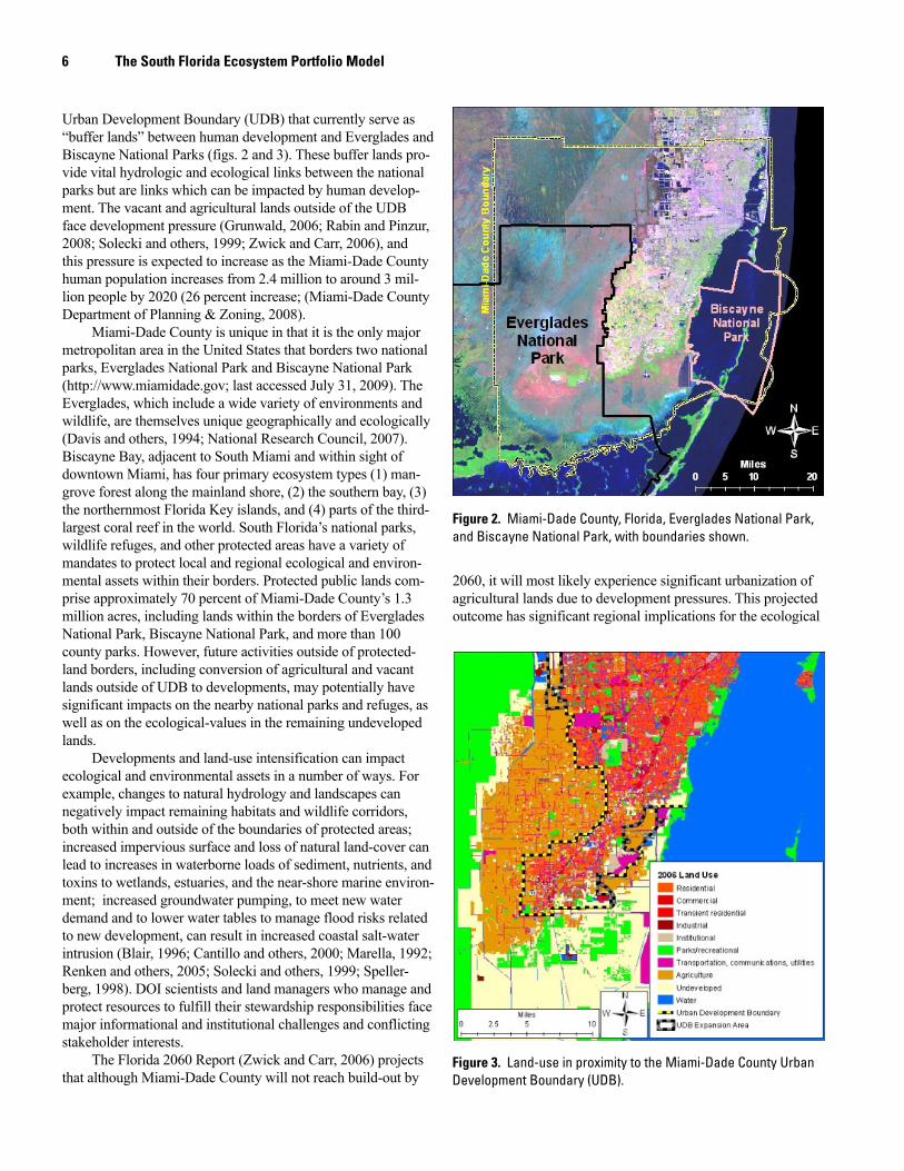
Figure 3. Land-use in proximity to the Miami-Dade County Urban Development Boundary (UDB).
2060, it will most likely experience significant urbanization of agricultural lands due to development pressures. This projected outcome has significant regional implications for the ecological
7
health of Everglades and Biscayne National Parks and the eco-logical functions served by the remaining vacant lands connect-ing the two parks (which includes other lands managed by the State and County), as well as implications for the well-being of Miami-Dade County residents. Although sea level rise impacts, including potential inundation of low-lying lands in Miami-Dade County, are not considered in the Florida 2060 Report, the interacting drivers of human population increases and sea level rise are of great concern to South Florida planners.
Future Work—Applying the EPM to Other Parts of South Florida
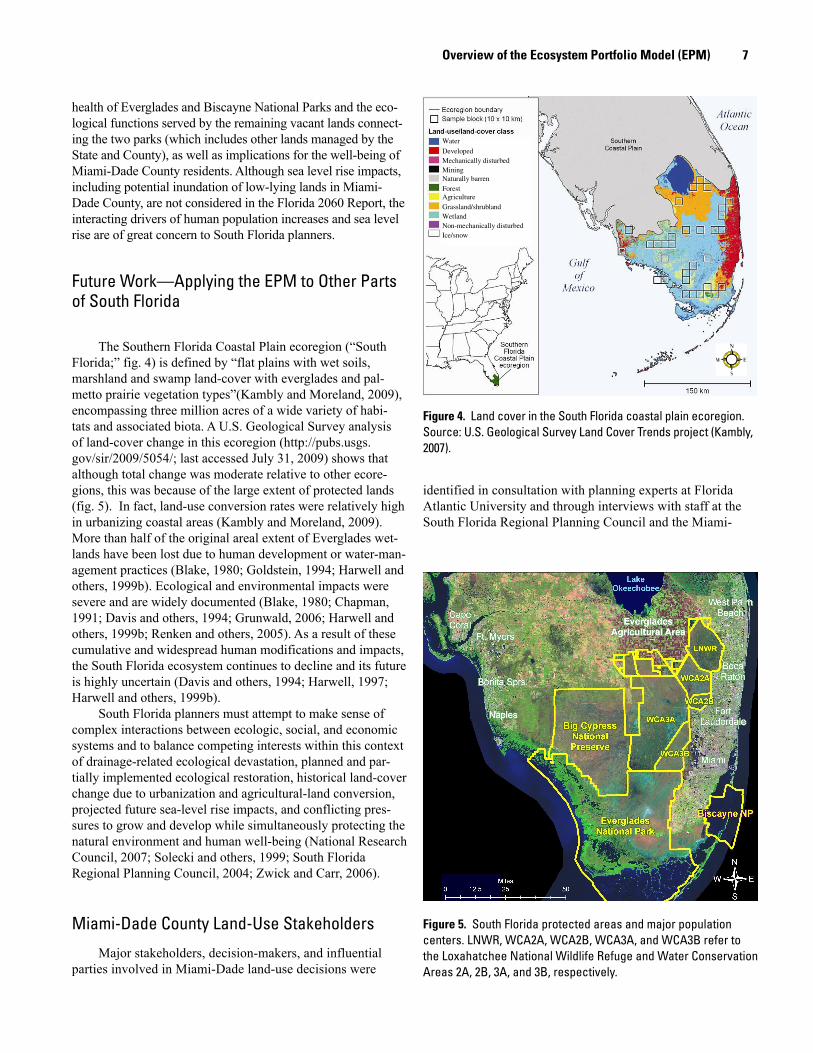
The Southern Florida Coastal Plain ecoregion (“South Florida;” fig. 4) is defined by “flat plains with wet soils, marshland and swamp land-cover with everglades and pal-metto prairie vegetation types”(Kambly and Moreland, 2009), encompassing three million acres of a wide variety of habi-tats and associated biota. A U.S. Geological Survey analysis of land-cover change in this ecoregion (http://pubs.usgs.gov/sir/2009/5054/; last accessed July 31, 2009) shows that although total change was moderate relative to other ecore-gions, this was because of the large extent of protected lands (fig. 5). In fact, land-use conversion rates were relatively high in urbanizing coastal areas (Kambly and Moreland, 2009). More than half of the original areal extent of Everglades wet-lands have been lost due to human development or water-man-agement practices (Blake, 1980; Goldstein, 1994; Harwell and others, 1999b). Ecological and environmental impacts were severe and are widely documented (Blake, 1980; Chapman, 1991; Davis and others, 1994; Grunwald, 2006; Harwell and others, 1999b; Renken and others, 2005). As a result of these cumulative and widespread human modifications and impacts, the South Florida ecosystem continues to decline and its future is highly uncertain (Davis and others, 1994; Harwell, 1997; Harwell and others, 1999b).
South Florida planners must attempt to make sense of complex interactions between ecologic, social, and economic systems and to balance competing interests within this context of drainage-related ecological devastation, planned and par-tially implemented ecological restoration, historical land-cover change due to urbanization and agricultural-land conversion, projected future sea-level rise impacts, and conflicting pres-sures to grow and develop while simultaneously protecting the natural environment and human well-being (National Research Council, 2007; Solecki and others, 1999; South Florida Regional Planning Council, 2004; Zwick and Carr, 2006).
Miami-Dade County Land-Use Stakeholders
Major stakeholders, decision-makers, and influential parties involved in Miami-Dade land-use decisions were
identified in consultation with planning experts at Florida Atlantic University and through interviews with staff at the South Florida Regional Planning Council and the Miami-
Figure 5. South Florida protected areas and major population centers. LNWR, WCA2A, WCA2B, WCA3A, and WCA3B refer to the Loxahatchee National Wildlife Refuge and Water Conservation Areas 2A, 2B, 3A, and 3B, respectively.
Overview of the Ecosystem Portfolio Model (EPM)
Non-mechanically disturbed Ice/snow
Wetland
Agriculture Grassland/shrubland
Forest Naturally barren Mining Mechanically disturbed Developed
Water
Figure 4. Land cover in the South Florida coastal plain ecoregion. Source: U.S. Geological Survey Land Cover Trends project (Kambly, 2007).
8 The South Florida Ecosystem Portfolio Model
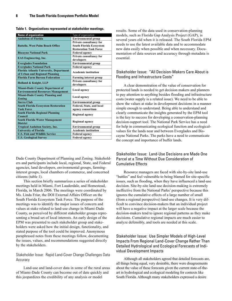
Dade County Department of Planning and Zoning. Stakehold-ers and participants include local, regional, State, and Federal agencies, land developers, environmental groups, farming-interest groups, local chambers of commerce, and concerned citizens (table 1).
This section briefly summarizes a series of stakeholder meetings held in Miami, Fort Lauderdale, and Homestead, Florida, in March 2006. The meetings were coordinated by Ms. Linda Friar, the DOI External Affairs Officer on the South Florida Ecosystem Task Force. The purpose of the meetings was to identify the major issues of concern and values at stake related to land-use change in Miami-Dade County, as perceived by different stakeholder groups repre-senting a broad set of local interests. An early design of the EPM was presented to each stakeholder group and stake-holders were asked how the initial design, functionality, and stated purpose of the tool could be improved. Anonymous paraphrased notes from these meetings follow, documenting the issues, values, and recommendations suggested directly by the stakeholders.
Stakeholder Issue: Rapid Land-Cover Change Challenges Data Accuracy
Land-use and land-cover data in some of the rural areas of Miami-Dade County can become out of date quickly and this jeopardizes the credibility of any analysis or model
results. Some of the data used in conservation-planning models, such as Florida Gap Analysis Project (GAP), is several years old when it is released. The South Florida EPM needs to use the latest available data and to accommodate new data easily when possible and when necessary. Docu-mentation of data sources and accuracy through metadata is essential.
Stakeholder Issue: “All Decision-Makers Care About is Flooding and Infrastructure Costs”
A clear demonstration of the value of conservation for protected lands is needed to get decision makers and planners to pay attention to anything besides flooding and infrastructure costs (water supply is a related issue). We need to be able to show the values at stake in development decisions in a manner simple enough to understand. Being able to understand and clearly communicate the insights generated by the EPM tool is the key to success for developing a conservation-planning decision-support tool. The National Park Service has a need for help in communicating ecological function and ecological-values for the lands near and between Everglades and Bis-cayne National Parks. The parks have a need to communicate the concept and importance of buffer lands.
Stakeholder Issue: Land-Use Decisions are Made One Parcel at a Time Without Due Consideration of Cumulative Effects
Resource managers are faced with site-by-site land-use “battles” and feel vulnerable to being blamed for site-specific issues, such as flooding, when they have influenced a land-use decision. Site-by-site land-use decision-making is extremely ineffective from the National Parks’ perspective because this ignores the cumulative effects of a large number of small (from a regional perspective) land-use changes. It is very dif-ficult to convince decision-makers that an individual project will have a negative impact at the larger scale because the decision-makers tend to ignore regional patterns as they make decisions. Cumulative regional impacts are much easier to analyze defensibly, and tools are needed at this scale.
Stakeholder Issue: Use Simpler Models of High-Level Impacts From Regional Land-Cover Change Rather Than Detailed Hydrological and Ecological Forecasts of Indi-vidual Development Impacts
Although all stakeholders agreed that detailed forecasts are, all things being equal, very desirable, there were disagreements about the value of these forecasts given the current state-of-the-art in hydrological and ecological modeling for contexts like South Florida. Although many stakeholders expressed a desire
Name of organization Type of organization Audubon of Florida Environmental group
Battelle, West Palm Beach Office
Private consultancy for
South Florida Ecosystem
Restoration Task Force
Biscayne National Park Federal agency
EAS Engineering, Inc. Private consultancy for
developers
Everglades Foundation Environmental group
Everglades National Park Federal agency
Florida Atlantic University, Department
of Urban and Regional Planning Academic institution
Florida Farm Bureau Federation Farming interest group
Holland & Knight, LLP Private consultancy for
developers
Miami-Dade County Department of
Environmental Resources Management Local agency
Miami-Dade County Planning and
Zoning Local agency
Sierra Club Environmental group
South Florida Ecosystem Restoration
Task Force
Federal, State, and local
agency consortium
South Florida Regional Planning
Council Regional agency
South Florida Water Management
District Regional agency
Tropical Audubon Society, Inc. Environmental group
University of Florida Academic institution
U.S. Fish and Wildlife Service Federal agency
U.S. Geological Survey Federal agency
Table 1. Organizations represented at stakeholder meetings.
9
for such forecasts, stakeholders with experience in such modeling strongly expressed the current limitations of using such forecasts for decision-support for land-use planning over decadal time hori-zons. Experts recognized that discussions would quickly become arguments about model assumptions, various uncertainties, and the trustworthiness of the forecasts, taking emphasis away from discussions about the importance of thinking regionally, the inher-ent tradeoffs involved, and other important issues.
Other issues and beliefs stated by stakeholders included:
• Development must be understood in terms of rev- enue generation. A municipality’s budget grows with new development through new tax revenues on retail, property, and other development. However, tax impli cations of the associated new infrastructure costs are not always recognized. • Water-supply considerations seem to trump ecologi cal considerations of local hydrology for Miami-Dade County decision-makers. This attitude is not shared by many stakeholders.
• The cumulative effects of development affect regional flood-control requirements; flood risk; storm-surge risk; potential hurricane losses; runoff and water- contaminant fluxes, including nutrients and sediment fluxes; reductions in wading-bird habitats; and reduc- tions in threatened and endangered-species habitats. • Moving the UDB, from the developer’s perspective, is about concurrency, that is, who pays for new infra- structure requirements associated with new develop- ment. Inside the UDB, taxpayers pay for the infrastruc- ture; outside the UDB, developers pay for it, so, devel- opers have a big incentive to support moving the UDB. • Protecting water wellfields (for seepage control, a form of flood control where groundwater tables are close to the surface) is a major local issue related to new development. • Although agricultural interests want to maintain agri cultural communities for as long as they can, they also want to retain the right to sell their lands to developers to maximize their land value. • Maintaining planned ecological-restoration-project footprints under the Comprehensive Everglades Restoration Plan is a major concern of the National Parks, since many of the needed lands have not yet been purchased. • Large numbers of new developments negate the ben eficial effects of past ecological-restoration efforts and decrease the potential effectiveness of future planned restoration efforts. This is largely ignored by local land- use decision-makers. • Issues of biological diversity and habitat/genetic diver- sity are usually ignored in land-use planning. • County planners want to hear about potential impacts of
planned developments on the National Parks, involving changes in impervious surface distribution, the ability to maintain park “gateways,” the “health and welfare” of the parks and refuges, the ability of the parks to meet their resource-protection mandates, tourism and park attendance, and the aesthetic appeal of the corridor between Everglades and Biscayne National Parks.• County planners want the National Parks to identify mitigation requirements associated with new develop- ments and to demonstrate potential long-term cumu lative impacts from new developments. However, as previously described, current practice often focuses on detailed analyses at small scales on a case-by-case basis. The National Parks and other stakeholders believe that larger-scale regional analyses are more appropriate.• The synthesis of any regional-scale evaluation of the impacts of new developments must be of use to county planners.
EPM Web-Enabled Model Interface
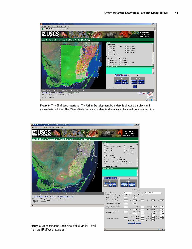
The EPM prototype is accessible through a password-protected, public Web interface developed using open-source GIS Web tools including Community Mapbuilder (http://communitymapbuilder.org/; last accessed July 31, 2009), Map Server (http://mapserver.gis.umn.edu/; last accessed July 31, 2009), and Tilecache (MetaCarta Labs; http://www.tilecache.org/; last accessed July 31, 2009). The EPM Web site includes a map viewer to display model inputs (land-use/cover maps) and outputs (ecological-value maps, land-price maps, and, in the future, human well-being metric maps), as well as other datasets and map layers that provide context for interpreting the models. For example, Landsat imagery, high-resolution orthoimagery, and contextual data such as the UDB, Urban Expansion Areas (UEA), roads, and managed-area boundaries, are available for display. From the Web interface, users are able to evaluate current landscapes, the 2025 and 2050 Watershed Study preferred scenarios, uploaded land-use plans developed by the user, and land-use plans made through modifications to any currently uploaded land-use map using the EPM interface.5 Other important land-use plans, like the Miami-Dade County Planning and Zoning Adopted 2015-2025 Land-use Plan Map, will be included in the future. The Web site prototype is shown in figure 6. The Web site will continue to be improved with additional criteria-based metrics and models, updated datasets, and refined functionality, based on user feedback and through future workshops during the second phase of the project.
Overview of the Ecosystem Portfolio Model (EPM)
5The South Miami-Dade Watershed Study and Plan is a regional planning effort undertaken by local and regional planning agencies and an advisory team that included stakeholders. Background information and results can be found at: http://southmiamidadewatershed.net/.
10 The South Florida Ecosystem Portfolio Model
The evaluations are based on the EVM (fig. 7), the market land-price model, and (in development) the community well-being model. The prototype has implemented models for all six of the EVM criteria, as well as the market land-price model. These models are currently being tested and evaluated by users at Everglades and Biscayne National Parks. The community well-being criteria models and datasets are beginning stages of design and are being developed in collaboration (ongoing) with researchers at Florida International University and Florida Atlantic University. Users will have the option of running the value map models for an area of interest or for the entire county, and will select multiattribute utility parameters (fig. 7) that reflect their priorities and values.
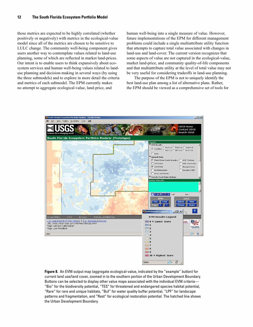
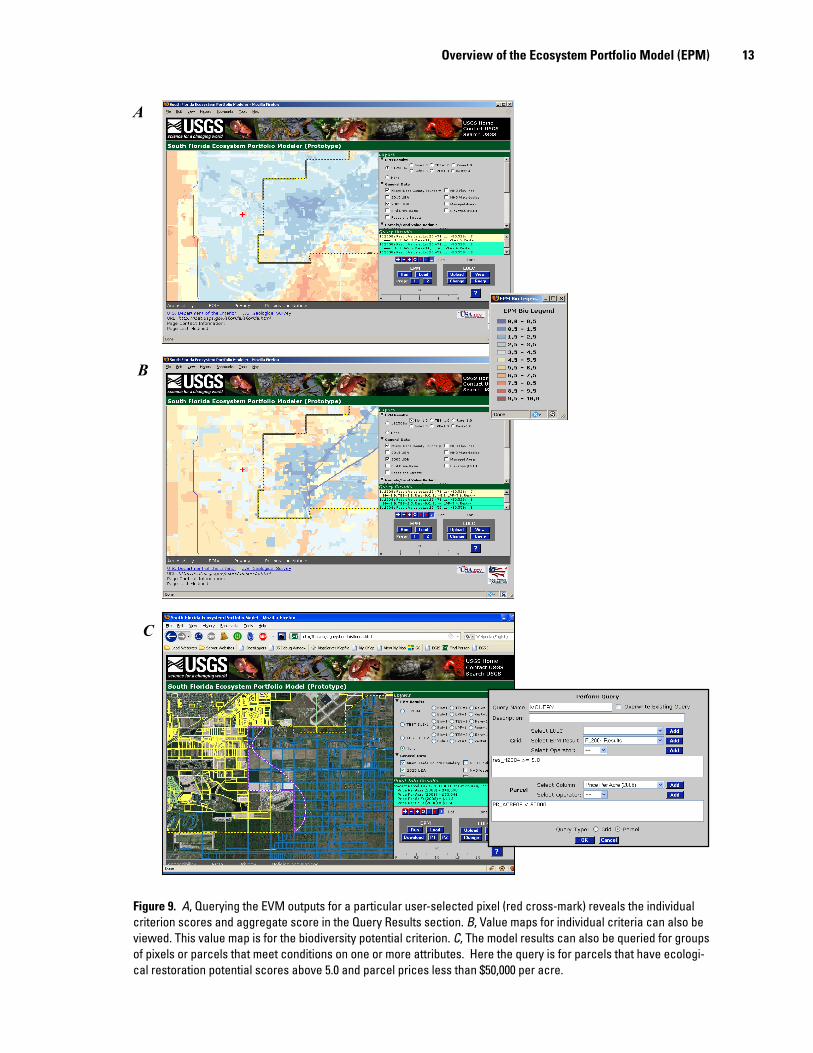
A raster grid of user-weighted ecological scores in a hypo-thetical user’s area of interest was generated using the EVM (fig. 7). In the current implementation, we assume that the ecological-value for each grid cell is equal to the sum of the weighted crite-ria values divided by the sum of the weights (arithmetic mean). Other methods of weighting and aggregating criteria will be explored in the future, since the appropriate procedure depends on the preferences of the user (for example, does a user’s prefer-ences for one criterion depend on the state of another criterion?), as well as the nature of the criteria themselves (are the criteria scores uncertain, and are they physically or biologically related to each other?). Each value-model criterion and the aggregate value (fig. 8) over all of the value-model’s criteria are listed on the Layers panel as buttons (fig. 8) that can be selected to display the associated value map. Users are able to query LULC classes, EVM and other model outputs, and other information at user-selected points using the interface. Users are also able to query model results to identify groups of cells and parcels that meet conditions of interest for inputs, outputs, or ancillary informa-tion. For example, the user can find cells or parcels that have EVM criteria scores above or below thresholds for cells cor-responding to parcels that also meet a land price threshold (fig. 9). All EPM model runs are saved for future retrieval, and can be accessed using the Load button.
Ecosystem Portfolio Model Compo-nents (Submodels), in Detail
This section describes each of the three major completed components (or submodels) of the South Florida Ecosystem Portfolio Model (1) the EVM, (2) the market LPM, and (3) the (human) community well-being model (WBM). The EVM and WBM are designed to evaluate land-use plans (LULC maps) in terms of spatially explicit metrics, each of which are related to one or more performance criteria, chosen to reflect Federal natural resource-management and regional- and county-plan-ning objectives. To avoid confusion, we distinguish between indicators and metrics in the following manner. An indicator is a summary of available data used to describe a current or historical characteristic of the natural (both abiotic and biotic)
or built environment and is defined such that it provides quantitative or qualitative information reflecting the current or historical state of the ecological or human social system (Mil-lennium Ecosystem Assessment, 2003; Morris and Therivel, 2009; Randolph, 2004). A metric, as used here, is a predic-tion (model output) of the future state of an indicator or other attribute of interest. In contrast, the LPM is a multivariate regression (hedonic) model that relates land-prices observed in markets to explanatory variables and, as such, is conceptu-ally different from the metric-based EVM and WBM models. Examples of explanatory variables include parcel characteris-tics and distances to amenities, as explained later.
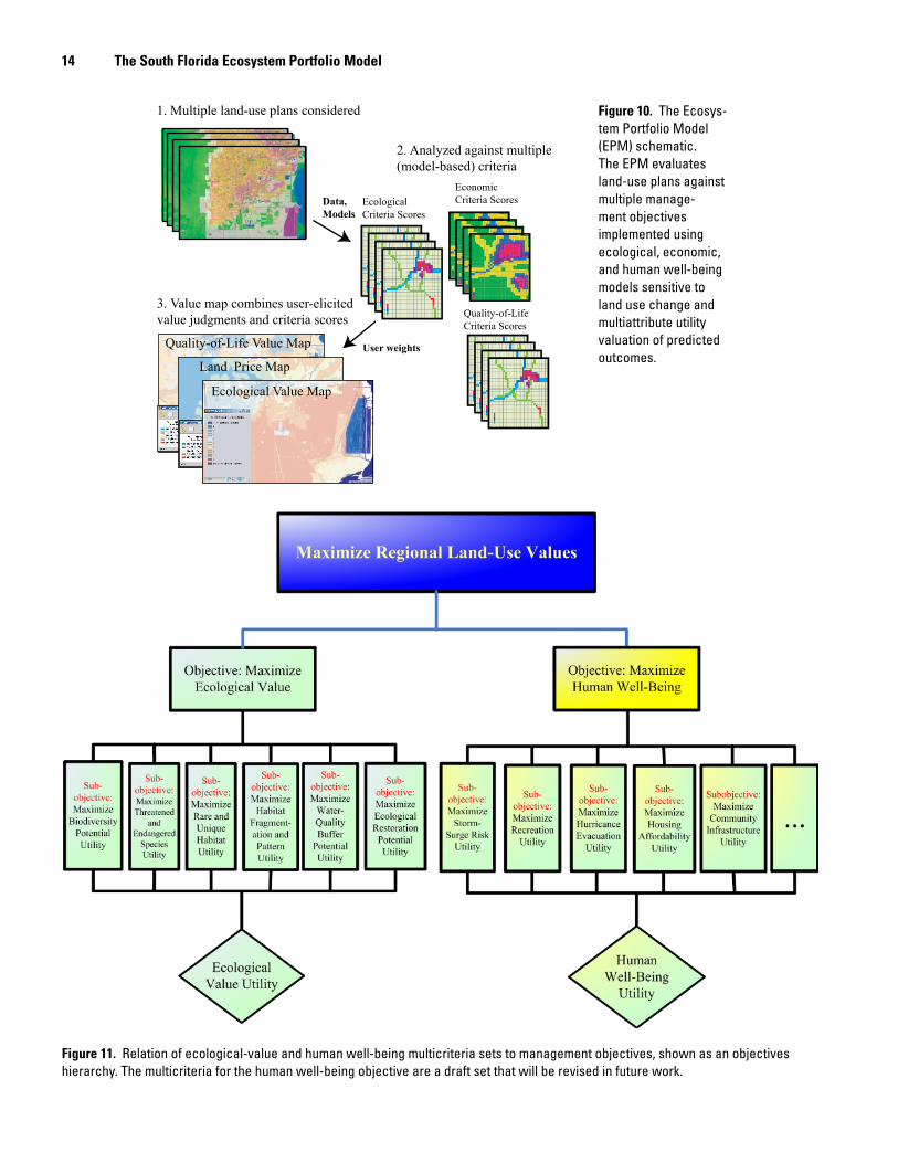
Through the use of this system of performance criteria, related metrics, and land price, the EPM partially decomposes “total value” related to land-use change into these various planning objectives (figs. 10 and 11). Because the perfor-mance criteria are chosen to be sensitive to land-cover change, they, of course, are physically dependent. Some of them are also preferentially dependent in that user preferences for particular bundles of criteria may demonstrate interactions between criteria. Also, there is no claim that the chosen criteria collectively exhaust total value, because this was not required for our case study. In fact, examples of value not reflected in any of them can easily be identified, for example, increased recreational values to visitors resulting from “green park entrances,” among many others.
The criteria, metrics, and models used for the EVM were chosen in collaboration with potential users and interested stakeholders and the WBM criteria, metrics, and models will be chosen in a similar process. The market land-price model is based on real estate market transaction data, parcel characteristic data, and other relevant data. Each of the EPM submodels was designed and implemented with the goal of finding an acceptable compromise between several competing objectives for evaluating land-use plans (1) credibility, (2) transparency, (3) flexibility, and (4) ease of use.
Ecological-value, as described later in this section, is defined by conservation and preservation objectives rooted in the mandates of the National Park Service, and the U.S. Fish and Wildlife Service, as well as in State and local resource-management objectives. The land-price model explores the value that the market places on some aspects of environmental and ecological goods and services, but important aspects of these goods and services are not reflected in the market price because they are “external” to the market. For example, deci-sions that can be expected to reduce these natural values may not reflect the costs associated with these reductions (Costanza and Folke, 1997; Goulder and Kennedy, 1997; Heal, 2000; Wilson and Carpenter, 1999). The ecological-value model is an attempt to quantify some of the nonmarket ecosystem and environmental values by using a multiattribute utility approach. Although the main purpose for the community well-being component is to allow users to focus on individual metrics of human well-being at the community scale, some of
11 Overview of the Ecosystem Portfolio Model (EPM)
Figure 6. The EPM Web Interface. The Urban Development Boundary is shown as a black and yellow hatched line. The Miami-Dade County boundary is shown as a black and gray hatched line.
Figure 7. Accessing the Ecological Value Model (EVM) from the EPM Web interface.
12 The South Florida Ecosystem Portfolio Model
those metrics are expected to be highly correlated (whether positively or negatively) with metrics in the ecological-value model since all of the metrics are chosen to be sensitive to LULC change. The community well-being component gives users another way to contemplate values related to land-use planning, some of which are reflected in market land-prices. Our intent is to enable users to think expansively about eco-system services and human well-being values related to land-use planning and decision-making in several ways (by using the three submodels) and to explore in more detail the criteria and metrics of each submodel. The EPM currently makes no attempt to aggregate ecological-value, land-price, and
human well-being into a single measure of value. However, future implementations of the EPM for different management problems could include a single multiattribute utility function that attempts to capture total value associated with changes in land-use and land-cover. The current version recognizes that some aspects of value are not captured in the ecological-value, market land-price, and community quality-of-life components and that multiattribute utility at the level of total value may not be very useful for considering tradeoffs in land-use planning.
The purpose of the EPM is not to uniquely identify the best land-use plan among a list of alternative plans. Rather, the EPM should be viewed as a comprehensive set of tools for
Figure 8. An EVM output map (aggregate ecological-value, indicated by the “example” button) for current land use/land cover, zoomed in to the southern portion of the Urban Development Boundary. Buttons can be selected to display other value maps associated with the individual EVM criteria—“Bio” for the biodiversity potential, “TES” for threatened and endangered species habitat potential, “Rare” for rare and unique habitats, “Buf” for water quality buffer potential, “LPF” for landscape patterns and fragmentation, and “Rest” for ecological restoration potential. The hatched line shows the Urban Development Boundary.
13 Overview of the Ecosystem Portfolio Model (EPM)
B
A
C
Figure 9. A, Querying the EVM outputs for a particular user-selected pixel (red cross-mark) reveals the individual criterion scores and aggregate score in the Query Results section. B, Value maps for individual criteria can also be viewed. This value map is for the biodiversity potential criterion. C, The model results can also be queried for groups of pixels or parcels that meet conditions on one or more attributes. Here the query is for parcels that have ecologi-cal restoration potential scores above 5.0 and parcel prices less than $50,000 per acre.
14 The South Florida Ecosystem Portfolio Model
1. Multiple land-use plans considered
2. Analyzed against multiple(model-based) criteria
Data,Models
Quality-of-LifeCriteria Scores
EconomicCriteria ScoresEcological
Criteria Scores
Quality-of-Life Value Map
Land Price Map
Ecological Value Map
User weights
3. Value map combines user-elicited value judgments and criteria scores
Figure 10. The Ecosys-tem Portfolio Model (EPM) schematic. The EPM evaluates land-use plans against multiple manage-ment objectives implemented using ecological, economic, and human well-being models sensitive to land use change and multiattribute utility valuation of predicted outcomes.
Figure 11. Relation of ecological-value and human well-being multicriteria sets to management objectives, shown as an objectives hierarchy. The multicriteria for the human well-being objective are a draft set that will be revised in future work.
15
exploratory use within a structured land-use planning process. The EPM should enlarge the debate by adding nested informa-tion from multiple perspectives and scales. By highlighting various sources of value and conflicting objectives, the EPM should allow users to explore spatially-explicit tradeoffs. The goal is to provide users with a better understanding of the many values at stake in land-use planning, some widely rec-ognized and reflected in the decision-making process, others largely ignored and external to the current decision-making process.
The Ecological-Value Submodel (EVM)
An Ecological-Value Model for Miami-Dade County Undeveloped Lands
The EVM a submodel of the EPM, is designed to evalu-ate land-use plans against several important ecological and environmental criteria (table 2) that reflect the resource-management priorities of the DOI. Although the EPM will ultimately be extended to other areas of South Florida, the current implementation focuses on the conservation, preser-vation, and restoration priorities of Everglades and Biscayne National Parks for lands in proximity to the parks within Miami-Dade County (figs. 1 and 4). The EVM criteria are defined to be sensitive to LULC change and are imple-mented through appropriate scoring models (table 2) that are accessed through the previously described GIS-based Web interface. Each criterion is scored for individual 30 by 30 m cells, where each cell’s score is determined by a model that uses the cell’s land-cover and other relevant model-specific characteristics as inputs. The models chosen to implement each criterion are based on existing models or accepted methods (table 2) and are described in the following sec-tions. Although most of the criteria are scored based on a cell’s local characteristics, a cell’s score for the landscape pattern and fragmenttion criterion is based on the land-cover patch configurations (identities and locations of patch land-cover classes) within a 1,200 m radius around that cell.6 The ecological-value map is a map of composite cell scores aggregated over each of the six criteria, where the multicri-teria aggregation process is based on a multiattribute utility (MAU) approach (Clemen, 1996; Edwards, 1977; Edwards and Hutton, 1994; Gregory, 1999). The advantage of a MAU approach is that it allows users to construct values “piece-
wise” within a cognitively complicated domain, through decomposition and reaggregation without the requirement for monetization.
The user can change the relative importance of each criterion by adjusting criteria weights. The weighted criteria scores are aggregated cell-wise using a MAU model that res-cales the original criterion scores to reflect user preferences and combines the individual scores in a way that reflects potential interactions between criteria (Clemen, 1996). As a concrete example, a cell with land-cover that corresponds to potential suitable habitat for one particular threatened and endangered (T&E) species would receive a score of “1,” for two T&E species, a score of “2,” and so forth. A MAU model approach allows the user to express that the “real” difference between a score of “0” (not suitable habitat for any T&E spe-cies) and “1” is greater than the difference between a score of “1” and “2”. In other words, the marginal utility over the scores decreases as the score increases. Ignoring decreasing marginal utility can result in anomalies when trying to com-bine scores between different criteria (Clemen, 1996).
Through the combined use of ecological-scoring models and MAU models, the EVM is an integration of the eco-logical sciences with the decision sciences to yield a robust LULC change evaluation tool. For example, sensitivity analysis can be performed to determine how sensitive aggre-gate ecological-value is to changes in the underlying MAU functions, user weights, the models used to characterize criteria attainment (table 2), and other assumptions. We now discuss the models, data, and methods used for each criterion of the EVM.
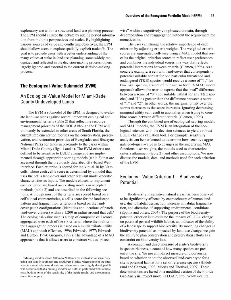
Ecological-Value Criterion 1—Biodiversity Potential
Biodiversity in sensitive natural areas has been observed to be significantly affected by encroachment of human land-use, due to habitat destruction, increase in habitat fragmenta-tion, and alteration of supporting environmental conditions (Eppink and others, 2004). The purpose of the biodiversity-potential criterion is to estimate the impacts of LULC change on potential general wildlife habitat, an indicator of the ability of a landscape to support biodiversity. By modeling changes in biodiversity potential as impacted by land-use change, we gain the ability to plan conservation and preservation efforts as a constraint on biodiversity loss.
A common and direct measure of a site’s biodiversity is species richness, a count of how many species are pres-ent at the site. We use an indirect measure of biodiversity, based on whether or not the observed land-cover type for a site is potential habitat for a set of reference species (Hildeb-rand and Cannon, 1993; Morris and Therivel, 2009). These determinations are based on a modified version of the Florida Gap Analysis Project model (FLGAP; http://www.wec.ufl.
Overview of the Ecosystem Portfolio Model (EPM)
6Moving windows from 600 m to 2000 m were evaluated for sensitivity using test sites in southeast and southwest Florida, where some of the sites were in a relatively natural state and others were more highly developed. It was determined that a moving window of 1,200 m performed well in these tests, both in terms of the sensitivity of the metric results and the computa-tional time required.
16 The South Florida Ecosystem Portfolio Model
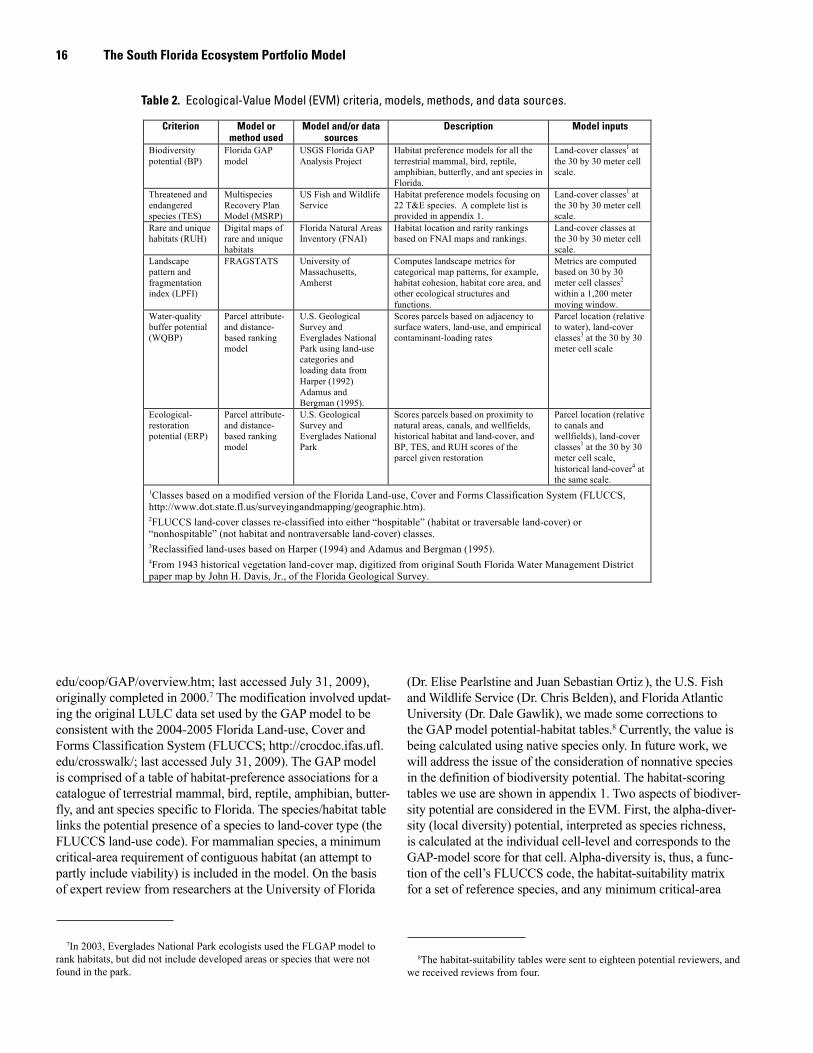
edu/coop/GAP/overview.htm; last accessed July 31, 2009), originally completed in 2000.7 The modification involved updat-ing the original LULC data set used by the GAP model to be consistent with the 2004-2005 Florida Land-use, Cover and Forms Classification System (FLUCCS; http://crocdoc.ifas.ufl.edu/crosswalk/; last accessed July 31, 2009). The GAP model is comprised of a table of habitat-preference associations for a catalogue of terrestrial mammal, bird, reptile, amphibian, butter-fly, and ant species specific to Florida. The species/habitat table links the potential presence of a species to land-cover type (the FLUCCS land-use code). For mammalian species, a minimum critical-area requirement of contiguous habitat (an attempt to partly include viability) is included in the model. On the basis of expert review from researchers at the University of Florida
(Dr. Elise Pearlstine and Juan Sebastian Ortiz ), the U.S. Fish and Wildlife Service (Dr. Chris Belden), and Florida Atlantic University (Dr. Dale Gawlik), we made some corrections to the GAP model potential-habitat tables.8 Currently, the value is being calculated using native species only. In future work, we will address the issue of the consideration of nonnative species in the definition of biodiversity potential. The habitat-scoring tables we use are shown in appendix 1. Two aspects of biodiver-sity potential are considered in the EVM. First, the alpha-diver-sity (local diversity) potential, interpreted as species richness, is calculated at the individual cell-level and corresponds to the GAP-model score for that cell. Alpha-diversity is, thus, a func-tion of the cell’s FLUCCS code, the habitat-suitability matrix for a set of reference species, and any minimum critical-area
Criterion Model or method used
Model and/or data sources
Description Model inputs
Biodiversity potential (BP)
Florida GAP model
USGS Florida GAP Analysis Project
Habitat preference models for all the terrestrial mammal, bird, reptile, amphibian, butterfly, and ant species in Florida.
Land-cover classes1 at the 30 by 30 meter cell scale.
Threatened and endangered species (TES)
Multispecies Recovery Plan Model (MSRP)
US Fish and Wildlife Service
Habitat preference models focusing on 22 T&E species. A complete list is provided in appendix 1.
Land-cover classes1 at the 30 by 30 meter cell scale.
Rare and unique habitats (RUH)
Digital maps of rare and unique habitats
Florida Natural Areas Inventory (FNAI)
Habitat location and rarity rankings based on FNAI maps and rankings.
Land-cover classes at the 30 by 30 meter cell scale.
Landscape pattern and fragmentation index (LPFI)
FRAGSTATS University of Massachusetts, Amherst
Computes landscape metrics for categorical map patterns, for example, habitat cohesion, habitat core area, and other ecological structures and functions.
Metrics are computed based on 30 by 30 meter cell classes2 within a 1,200 meter moving window.
Water-quality buffer potential (WQBP)
Parcel attribute-and distance-based ranking model
U.S. Geological Survey and Everglades National Park using land-use categories and loading data from Harper (1992) Adamus and Bergman (1995).
Scores parcels based on adjacency to surface waters, land-use, and empirical contaminant-loading rates
Parcel location (relative to water), land-cover classes3 at the 30 by 30 meter cell scale
Ecological-restoration potential (ERP)
Parcel attribute-and distance-based ranking model
U.S. Geological Survey and Everglades National Park
Scores parcels based on proximity to natural areas, canals, and wellfields, historical habitat and land-cover, and BP, TES, and RUH scores of the parcel given restoration
Parcel location (relative to canals and wellfields), land-cover classes1 at the 30 by 30 meter cell scale, historical land-cover4 at the same scale.
1Classes based on a modified version of the Florida Land-use, Cover and Forms Classification System (FLUCCS, http://www.dot.state.fl.us/surveyingandmapping/geographic.htm). 2FLUCCS land-cover classes re-classified into either “hospitable” (habitat or traversable land-cover) or “nonhospitable” (not habitat and nontraversable land-cover) classes. 3Reclassified land-uses based on Harper (1994) and Adamus and Bergman (1995). 4From 1943 historical vegetation land-cover map, digitized from original South Florida Water Management District paper map by John H. Davis, Jr., of the Florida Geological Survey.
Table 2. Ecological-Value Model (EVM) criteria, models, methods, and data sources.
7In 2003, Everglades National Park ecologists used the FLGAP model to rank habitats, but did not include developed areas or species that were not found in the park.
8The habitat-suitability tables were sent to eighteen potential reviewers, and we received reviews from four.
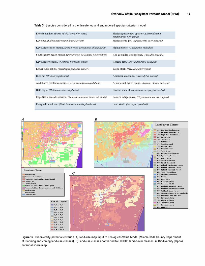
17 Overview of the Ecosystem Portfolio Model (EPM)
Land-use Classes
A Land-cover Classes
B
C
Figure 12. Biodiversity-potential criterion. A, Land-use map input to Ecological-Value Model (Miami-Dade County Department of Planning and Zoning land-use classes). B, Land-use classes converted to FLUCCS land-cover classes. C, Biodiversity (alpha) potential score map.
Florida panther, (Puma [Felis] concolor coryi) Florida grasshopper sparrow, (Ammodramus
savannarum floridanus)
Key deer, (Odocoileus virginianus clavium) Florida scrub-jay, (Aphelocoma coerulescens)
Key Largo cotton mouse, (Peromyscus gossypinus allapaticola) Piping plover, (Charadrius melodus)
Southeastern beach mouse, (Peromyscus polionotus niveiventris) Red-cockaded woodpecker, (Picoides borealis)
Key Largo woodrat, (Neotoma floridana smalli) Roseate tern, (Sterna dougallii dougallii)
Lower Keys rabbit, (Sylvilagus palustris hefneri) Wood stork, (Mycteria americana)
Rice rat, (Oryzomys palustris) American crocodile, (Crocodylus acutus)
Audubon’s crested caracara, (Polyborus plancus audubonii) Atlantic salt marsh snake, (Nerodia clarkii taeniata)
Bald eagle, (Haliaeetus leucocephalus) Bluetail mole skink, (Eumeces egregius lividus)
Cape Sable seaside sparrow, (Ammodramus maritimus mirabilis) Eastern indigo snake, (Drymarchon corais couperi)
Everglade snail kite, (Rostrhamus sociabilis plumbeus) Sand skink, (Neoseps reynoldsi)
Table 3. Species considered in the threatened and endangered species criterion model.
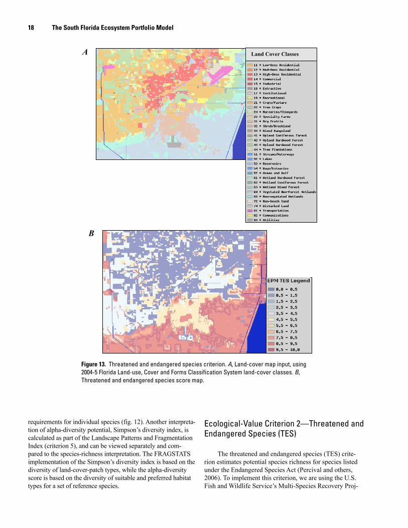
18 The South Florida Ecosystem Portfolio Model
requirements for individual species (fig. 12). Another interpreta-tion of alpha-diversity potential, Simpson’s diversity index, is calculated as part of the Landscape Patterns and Fragmentation Index (criterion 5), and can be viewed separately and com-pared to the species-richness interpretation. The FRAGSTATS implementation of the Simpson’s diversity index is based on the diversity of land-cover-patch types, while the alpha-diversity score is based on the diversity of suitable and preferred habitat types for a set of reference species.
Ecological-Value Criterion 2—Threatened and Endangered Species (TES)
The threatened and endangered species (TES) crite-rion estimates potential species richness for species listed under the Endangered Species Act (Percival and others, 2006). To implement this criterion, we are using the U.S. Fish and Wildlife Service’s Multi-Species Recovery Proj-
A Land Cover Classes
B
Figure 13. Threatened and endangered species criterion. A, Land-cover map input, using 2004-5 Florida Land-use, Cover and Forms Classification System land-cover classes. B, Threatened and endangered species score map.
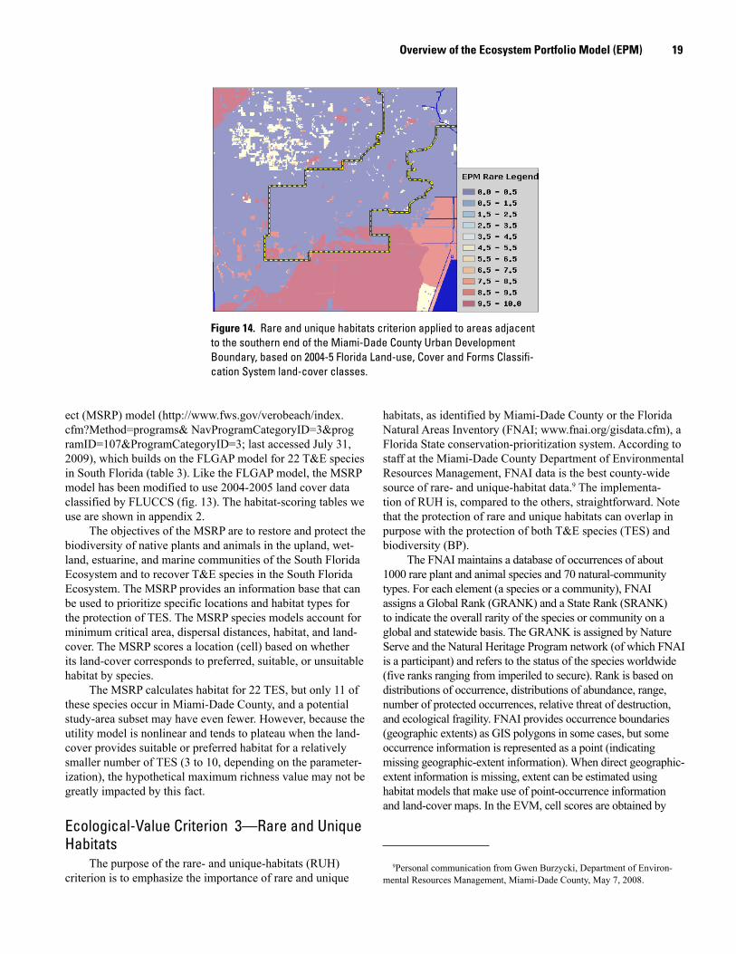
19
ect (MSRP) model (http://www.fws.gov/verobeach/index.cfm?Method=programs& NavProgramCategoryID=3&programID=107&ProgramCategoryID=3; last accessed July 31, 2009), which builds on the FLGAP model for 22 T&E species in South Florida (table 3). Like the FLGAP model, the MSRP model has been modified to use 2004-2005 land cover data classified by FLUCCS (fig. 13). The habitat-scoring tables we use are shown in appendix 2.
The objectives of the MSRP are to restore and protect the biodiversity of native plants and animals in the upland, wet-land, estuarine, and marine communities of the South Florida Ecosystem and to recover T&E species in the South Florida Ecosystem. The MSRP provides an information base that can be used to prioritize specific locations and habitat types for the protection of TES. The MSRP species models account for minimum critical area, dispersal distances, habitat, and land-cover. The MSRP scores a location (cell) based on whether its land-cover corresponds to preferred, suitable, or unsuitable habitat by species.
The MSRP calculates habitat for 22 TES, but only 11 of these species occur in Miami-Dade County, and a potential study-area subset may have even fewer. However, because the utility model is nonlinear and tends to plateau when the land-cover provides suitable or preferred habitat for a relatively smaller number of TES (3 to 10, depending on the parameter-ization), the hypothetical maximum richness value may not be greatly impacted by this fact.
Ecological-Value Criterion 3—Rare and Unique Habitats
The purpose of the rare- and unique-habitats (RUH) criterion is to emphasize the importance of rare and unique
habitats, as identified by Miami-Dade County or the Florida Natural Areas Inventory (FNAI; www.fnai.org/gisdata.cfm), a Florida State conservation-prioritization system. According to staff at the Miami-Dade County Department of Environmental Resources Management, FNAI data is the best county-wide source of rare- and unique-habitat data.9 The implementa-tion of RUH is, compared to the others, straightforward. Note that the protection of rare and unique habitats can overlap in purpose with the protection of both T&E species (TES) and biodiversity (BP).
The FNAI maintains a database of occurrences of about 1000 rare plant and animal species and 70 natural-community types. For each element (a species or a community), FNAI assigns a Global Rank (GRANK) and a State Rank (SRANK) to indicate the overall rarity of the species or community on a global and statewide basis. The GRANK is assigned by Nature Serve and the Natural Heritage Program network (of which FNAI is a participant) and refers to the status of the species worldwide (five ranks ranging from imperiled to secure). Rank is based on distributions of occurrence, distributions of abundance, range, number of protected occurrences, relative threat of destruction, and ecological fragility. FNAI provides occurrence boundaries (geographic extents) as GIS polygons in some cases, but some occurrence information is represented as a point (indicating missing geographic-extent information). When direct geographic-extent information is missing, extent can be estimated using habitat models that make use of point-occurrence information and land-cover maps. In the EVM, cell scores are obtained by
Overview of the Ecosystem Portfolio Model (EPM)
Figure 14. Rare and unique habitats criterion applied to areas adjacent to the southern end of the Miami-Dade County Urban Development Boundary, based on 2004-5 Florida Land-use, Cover and Forms Classifi-cation System land-cover classes.
9Personal communication from Gwen Burzycki, Department of Environ-mental Resources Management, Miami-Dade County, May 7, 2008.
20 The South Florida Ecosystem Portfolio Model
overlaying the FNAI Rare Species Habitat Conservation Priorities map over the cell grid and transferring direct or estimated poly-gon scores to the grid cells. This data layer provides an inventory of places on the landscape that would protect rare and endangered species based on known occurrences (fig. 14).
Ecological-Value Criterion 4—Water-Quality Buffer Potential
The water-quality buffer potential (WQBP) criterion examines land-use adjacent to and near surface-water conduits (often canals in Miami-Dade County, some navigable, some not) and considers the potential effects of different land-uses in this area on downstream water-quality. The WQBP criterion focuses on LULC attributes that tend to improve or degrade water-quality and is modeled based on empirical relationships between LULC types, distances to surface-water conduits, and estimated contaminant loadings. In general, we assign a score based on distinct LULC and distance for each cell in a defined buffer zone around surface-water features (for example, canals, lakes, wetlands) separately for total nitrogen (TN), total phos-phorus (TP), and suspended sediment (SS). The scores for the three pollutants are weighted by the user and combined to pro-vide the overall score, where the weights reflect the importance of each contaminant in terms of management objectives.
The buffer zone around the surface-water bodies (for example, canals, lakes, wetlands) was delineated using the USGS National Hydrography dataset. Buffers were defined as 500 feet (about 152 m) on all sides to provide a conserva-tive estimate, based on local work by the Miami Conservancy (http://www.miamiconservancy.org/flood/pdfs/riparian_buffers.pdf; last accessed July 31, 2009). Since a cell in our analysis is 30 by 30 m, the buffer zone was 5 cells across on either side of the canal or surface-water body. We used a linear attenuation factor based on the number of cells from the con-
tamination source cell being scored to the closest surface-water conduit.
We reclassified the FLUCCS codes into 14 categories as shown in table 4 (Adamus and Bergman, 1995). The reclassi-fied FLUCCS codes were then related to mean pollutant con-centrations commonly found in runoff in south Florida based on different land-uses (Adamus and Bergman, 1995); table 5). We normalized each of the mean pollutant concentrations to relative values so that we could compare the three pollutants together in the WQBP criterion. For each pollutant, for each land-use, a normalized value is derived by subtracting the con-centration value from the lowest concentration value, and then dividing by the standard deviation of the all the values for that pollutant (table 5). Scoring for the WQBP criterion is done for each cell, k, in the buffer zone individually for TN, TP, and SS. The final score is a user-weighted average of the three scores for TN, TP, and SS, defined by:
ScoreWQ,k = , (1)
where wD is the attenuation factor based on distance from canal, wj is the user-adjusted weight for contaminant j, j Є {TN, TP, SS}, and Nj,l is a normalized concentration value for contaminant j and land-use type l.
Ecological-Value Criterion 5—Landscape Pat-terns and Fragmentation Index
The landscape patterns and fragmentation index (LPFI) refers to an aggregate of individual landscape-ecological metrics, each of which focuses on different aspects of the
Distance
(cells)
1 2 3 4 5 61
Attenuation
factor
1 0.833 0.667 0.5 0.333 0.167
1Although the buffer zone is 5 cells, the analysis requires six cells to account for the cell
containing the canal or the edge of the water body.
All other cells in the study area (outside of the 500-foot buffer) receive an attenuation factor of 0 and, thus, are not considered in the WQBP criterion.
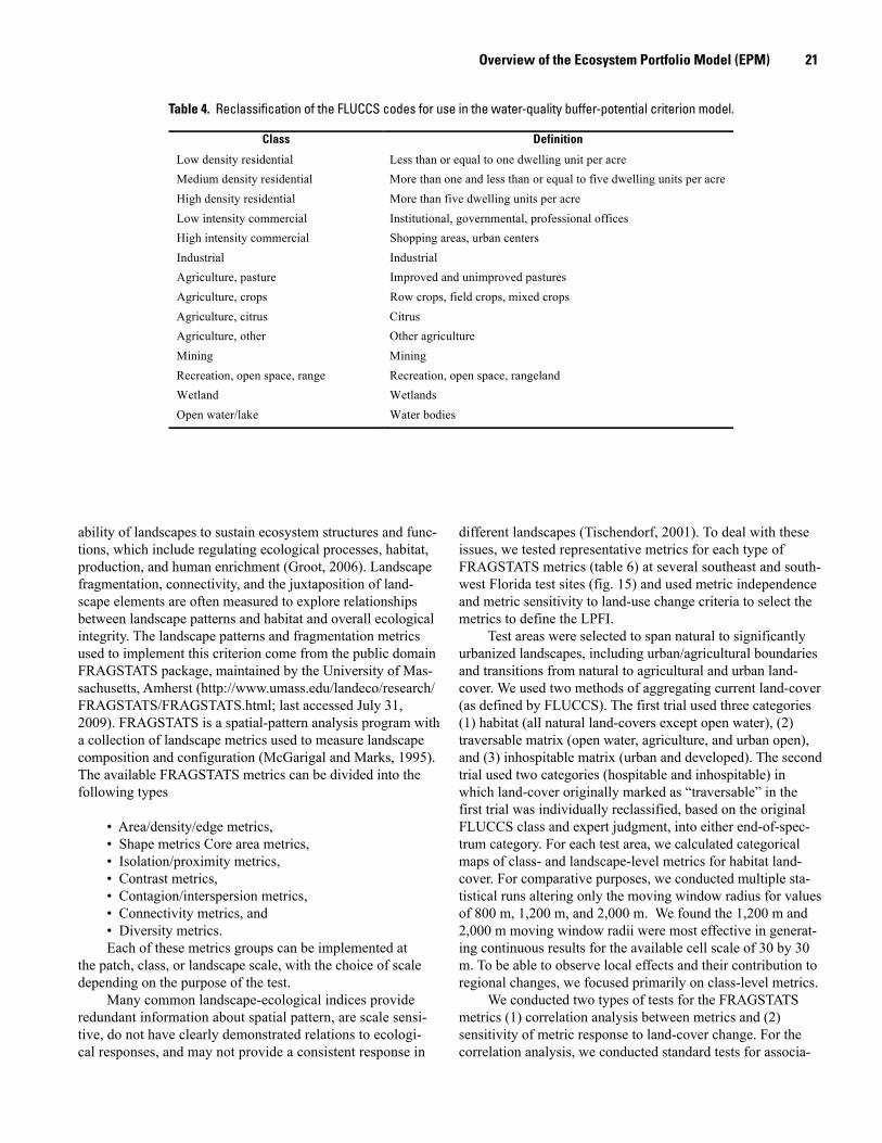
21 Overview of the Ecosystem Portfolio Model (EPM)
ability of landscapes to sustain ecosystem structures and func-tions, which include regulating ecological processes, habitat, production, and human enrichment (Groot, 2006). Landscape fragmentation, connectivity, and the juxtaposition of land-scape elements are often measured to explore relationships between landscape patterns and habitat and overall ecological integrity. The landscape patterns and fragmentation metrics used to implement this criterion come from the public domain FRAGSTATS package, maintained by the University of Mas-sachusetts, Amherst (http://www.umass.edu/landeco/research/FRAGSTATS/FRAGSTATS.html; last accessed July 31, 2009). FRAGSTATS is a spatial-pattern analysis program with a collection of landscape metrics used to measure landscape composition and configuration (McGarigal and Marks, 1995). The available FRAGSTATS metrics can be divided into the following types
• Area/density/edge metrics, • Shape metrics Core area metrics,• Isolation/proximity metrics,• Contrast metrics,• Contagion/interspersion metrics,• Connectivity metrics, and• Diversity metrics.Each of these metrics groups can be implemented at
the patch, class, or landscape scale, with the choice of scale depending on the purpose of the test.
Many common landscape-ecological indices provide redundant information about spatial pattern, are scale sensi-tive, do not have clearly demonstrated relations to ecologi-cal responses, and may not provide a consistent response in
different landscapes (Tischendorf, 2001). To deal with these issues, we tested representative metrics for each type of FRAGSTATS metrics (table 6) at several southeast and south-west Florida test sites (fig. 15) and used metric independence and metric sensitivity to land-use change criteria to select the metrics to define the LPFI.
Test areas were selected to span natural to significantly urbanized landscapes, including urban/agricultural boundaries and transitions from natural to agricultural and urban land-cover. We used two methods of aggregating current land-cover (as defined by FLUCCS). The first trial used three categories (1) habitat (all natural land-covers except open water), (2) traversable matrix (open water, agriculture, and urban open), and (3) inhospitable matrix (urban and developed). The second trial used two categories (hospitable and inhospitable) in which land-cover originally marked as “traversable” in the first trial was individually reclassified, based on the original FLUCCS class and expert judgment, into either end-of-spec-trum category. For each test area, we calculated categorical maps of class- and landscape-level metrics for habitat land-cover. For comparative purposes, we conducted multiple sta-tistical runs altering only the moving window radius for values of 800 m, 1,200 m, and 2,000 m. We found the 1,200 m and 2,000 m moving window radii were most effective in generat-ing continuous results for the available cell scale of 30 by 30 m. To be able to observe local effects and their contribution to regional changes, we focused primarily on class-level metrics.
We conducted two types of tests for the FRAGSTATS metrics (1) correlation analysis between metrics and (2) sensitivity of metric response to land-cover change. For the correlation analysis, we conducted standard tests for associa-
Class Definition
Low density residential Less than or equal to one dwelling unit per acre Medium density residential More than one and less than or equal to five dwelling units per acre High density residential More than five dwelling units per acre Low intensity commercial Institutional, governmental, professional offices High intensity commercial Shopping areas, urban centers Industrial Industrial Agriculture, pasture Improved and unimproved pastures Agriculture, crops Row crops, field crops, mixed crops Agriculture, citrus Citrus Agriculture, other Other agriculture Mining Mining Recreation, open space, range Recreation, open space, rangeland Wetland Wetlands Open water/lake Water bodies
Table 4. Reclassification of the FLUCCS codes for use in the water-quality buffer-potential criterion model.
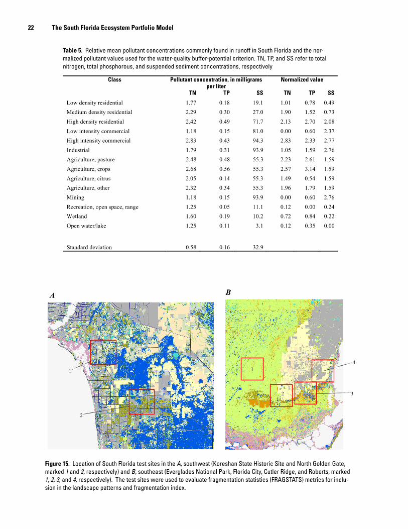
22 The South Florida Ecosystem Portfolio Model
Figure 15. Location of South Florida test sites in the A, southwest (Koreshan State Historic Site and North Golden Gate, marked 1 and 2, respectively) and B, southeast (Everglades National Park, Florida City, Cutler Ridge, and Roberts, marked 1, 2, 3, and 4, respectively). The test sites were used to evaluate fragmentation statistics (FRAGSTATS) metrics for inclu-sion in the landscape patterns and fragmentation index.
Class Pollutant concentration, in milligrams per liter
Normalized value
TN TP SS TN TP SS
Low density residential 1.77 0.18 19.1 1.01 0.78 0.49 Medium density residential 2.29 0.30 27.0 1.90 1.52 0.73 High density residential 2.42 0.49 71.7 2.13 2.70 2.08 Low intensity commercial 1.18 0.15 81.0 0.00 0.60 2.37 High intensity commercial 2.83 0.43 94.3 2.83 2.33 2.77 Industrial 1.79 0.31 93.9 1.05 1.59 2.76 Agriculture, pasture 2.48 0.48 55.3 2.23 2.61 1.59 Agriculture, crops 2.68 0.56 55.3 2.57 3.14 1.59 Agriculture, citrus 2.05 0.14 55.3 1.49 0.54 1.59 Agriculture, other 2.32 0.34 55.3 1.96 1.79 1.59 Mining 1.18 0.15 93.9 0.00 0.60 2.76 Recreation, open space, range 1.25 0.05 11.1 0.12 0.00 0.24 Wetland 1.60 0.19 10.2 0.72 0.84 0.22 Open water/lake 1.25 0.11 3.1 0.12 0.35 0.00
Standard deviation 0.58 0.16 32.9
Table 5. Relative mean pollutant concentrations commonly found in runoff in South Florida and the nor-malized pollutant values used for the water-quality buffer-potential criterion. TN, TP, and SS refer to total nitrogen, total phosphorous, and suspended sediment concentrations, respectively
1
2
1
2 3
4
A B
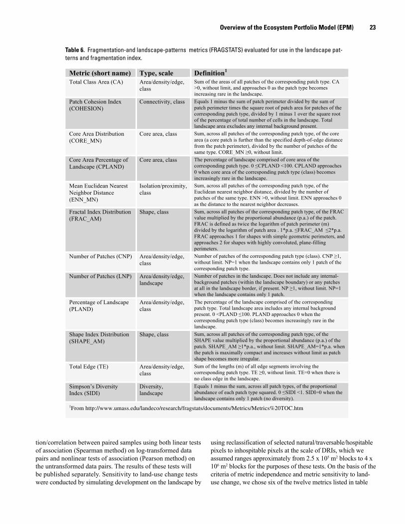
23 Overview of the Ecosystem Portfolio Model (EPM)
Metric (short name) Type, scale Definition1
Total Class Area (CA) Area/density/edge,class
Sum of the areas of all patches of the corresponding patch type. CA >0, without limit, and approaches 0 as the patch type becomes increasing rare in the landscape.
Patch Cohesion Index (COHESION)
Connectivity, class Equals 1 minus the sum of patch perimeter divided by the sum of patch perimeter times the square root of patch area for patches of the corresponding patch type, divided by 1 minus 1 over the square root of the percentage of total number of cells in the landscape. Total landscape area excludes any internal background present.
Core Area Distribution (CORE_MN)
Core area, class Sum, across all patches of the corresponding patch type, of the core area (a core patch is further than the specified depth-of-edge distance from the patch perimeter), divided by the number of patches of the same type. CORE_MN 0, without limit.
Core Area Percentage of Landscape (CPLAND)
Core area, class The percentage of landscape comprised of core area of the corresponding patch type. 0 CPLAND <100. CPLAND approaches 0 when core area of the corresponding patch type (class) becomes increasingly rare in the landscape.
Mean Euclidean Nearest Neighbor Distance (ENN_MN)
Isolation/proximity, class
Sum, across all patches of the corresponding patch type, of the Euclidean nearest neighbor distance, divided by the number of patches of the same type. ENN >0, without limit. ENN approaches 0 as the distance to the nearest neighbor decreases.
Fractal Index Distribution (FRAC_AM)
Shape, class Sum, across all patches of the corresponding patch type, of the FRAC value multiplied by the proportional abundance (p.a.) of the patch. FRAC is defined as twice the logarithm of patch perimeter (m) divided by the logarithm of patch area . 1*p.a. FRAC_AM 2*p.a. FRAC approaches 1 for shapes with simple geometric perimeters, and approaches 2 for shapes with highly convoluted, plane-filling perimeters.
Number of Patches (CNP) Area/density/edge,class
Number of patches of the corresponding patch type (class). CNP 1, without limit. NP=1 when the landscape contains only 1 patch of the corresponding patch type.
Number of Patches (LNP) Area/density/edge,landscape
Number of patches in the landscape. Does not include any internal-background patches (within the landscape boundary) or any patches at all in the landscape border, if present. NP 1, without limit. NP=1 when the landscape contains only 1 patch.
Percentage of Landscape (PLAND)
Area/density/edge,class
The percentage of the landscape comprised of the corresponding patch type. Total landscape area includes any internal background present. 0 <PLAND 100. PLAND approaches 0 when the corresponding patch type (class) becomes increasingly rare in the landscape.
Shape Index Distribution (SHAPE_AM)
Shape, class Sum, across all patches of the corresponding patch type, of the SHAPE value multiplied by the proportional abundance (p.a.) of the patch. SHAPE_AM 1*p.a., without limit. SHAPE_AM=1*p.a. when the patch is maximally compact and increases without limit as patch shape becomes more irregular.
Total Edge (TE) Area/density/edge,class
Sum of the lengths (m) of all edge segments involving the corresponding patch type. TE 0, without limit. TE=0 when there is no class edge in the landscape.
Simpson’s Diversity Index (SIDI)
Diversity, landscape
Equals 1 minus the sum, across all patch types, of the proportional abundance of each patch type squared. 0 SIDI <1. SIDI=0 when the landscape contains only 1 patch (no diversity).
1From http://www.umass.edu/landeco/research/fragstats/documents/Metrics/Metrics%20TOC.htm
Table 6. Fragmentation-and landscape-patterns metrics (FRAGSTATS) evaluated for use in the landscape pat-terns and fragmentation index.
tion/correlation between paired samples using both linear tests of association (Spearman method) on log-transformed data pairs and nonlinear tests of association (Pearson method) on the untransformed data pairs. The results of these tests will be published separately. Sensitivity to land-use change tests were conducted by simulating development on the landscape by
using reclassification of selected natural/traversable/hospitable pixels to inhospitable pixels at the scale of DRIs, which we assumed ranges approximately from 2.5 x 10⁵ m2 blocks to 4 x 10⁶ m2 blocks for the purposes of these tests. On the basis of the criteria of metric independence and metric sensitivity to land-use change, we chose six of the twelve metrics listed in table
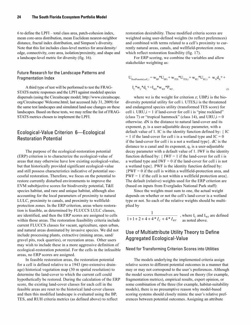
24 The South Florida Ecosystem Portfolio Model
6 to define the LPFI – total class area, patch-cohesion index, mean core-area distribution, mean Euclidean nearest-neighbor distance, fractal index distribution, and Simpson’s diversity. Note that this list includes class-level metrics for area/density/edge, connectivity, core area, isolation/proximity, and shape and a landscape-level metric for diversity (fig. 16).
Future Research for the Landscape Patterns and Fragmentation Index
A third type of test will be performed to test the FRAG-STATS metric responses and the LPFI against modeled species dispersals (using the Circuitscape model; http://www.circuitscape.org/Circuitscape/ Welcome.html; last accessed July 31, 2009) for the same test landscapes and simulated land-use changes on these landscapes. Based on these tests, we may refine the list of FRAG-STATS metrics chosen to implement the LPFI.
Ecological-Value Criterion 6—Ecological Restoration Potential
The purpose of the ecological-restoration potential (ERP) criterion is to characterize the ecological-value of areas that may otherwise have low existing ecological-value, but that historically provided significant ecological-value and still possess characteristics indicative of potential suc-cessful restoration. Therefore, we focus on the potential to restore currently disturbed environments to improve the EVM subobjective scores for biodiversity potential, T&E species habitat, and rare and unique habitat, although also accounting for the local parameters of proximity to natural LULC, proximity to canals, and proximity to wellfield-protection zones. In the ERP criterion, areas where restora-tion is feasible, as determined by FLUCCS LULC classes, are identified, and then the ERP scores are assigned to cells within those areas. The restoration feasibility criteria include current FLUCCS classes for vacant, agriculture, open urban, and natural areas dominated by invasive species. We did not include processing plants, extractive (mining areas, sand/gravel pits, rock quarries), or recreation areas. Other users may wish to include these in a more aggressive definition of ecological-restoration potential. For the cells in the infeasible areas, no ERP scores are assigned.
In feasible restoration areas, the restoration potential for a cell is defined relative to a 1943 (pre-extensive drain-age) historical vegetation map (30 m spatial resolution) to determine the land-cover to which the current cell could hypothetically be restored. During the calculation of the ERP score, the existing land-cover classes for each cell in the feasible areas are reset to the historical land-cover classes and then this modified landscape is evaluated using the BP, TES, and RUH criteria metrics (as defined above) to reflect
restoration desirability. These modified criteria scores are weighted using user-defined weights (to reflect preferences) and combined with terms related to a cell’s proximity to cur-rently natural areas, canals, and wellfield-protection zones, which reflect restoration feasibility (fig. 17).
For ERP scoring, we combine the variables and allow stakeholder weighting as:
URestPotential,cell_i = wBP*UBP,i + wTES*UTES,i + wRU*URU,i + wNdN-p +
IC*wC*dC-q +IWF*wWF*PWF , (2)
where wz is the weight for criterion z; UBP,i is the bio-diversity potential utility for cell i. UTES,i is the threatened and endangered species utility (transformed TES score) for cell i. URU,i = 1 if land-cover for cell i is “pine rockland” (class 7) or “tropical hammock” (class 14), and URU,i = 0 otherwise. dN is the distance to natural land-cover and its exponent, p, is a user-adjustable decay parameter, with a default value of 1. IC is the identity function defined by: { IC = 1 if the land-cover for cell i is a wetland type and IC = 0 if the land-cover for cell i is a not a wetland type}. dC is the distance to a canal and its exponent, q, is a user-adjustable decay parameter with a default value of 1. IWF is the identity function defined by: { IWF = 1 if the land-cover for cell i is a wetland type and IWF = 0 if the land-cover for cell i is not a wetland type}. PWF is the identity function defined by: {PWF = 0 if the cell is within a wellfield-protection area, and PWF = 1 if the cell is not within a wellfield protection area}. The default (relative) weights used for the ERP criterion are (based on inputs from Everglades National Park staff):
Since the weights must sum to one, the actual weight depends on whether or not the cell’s land-cover is a wetland type or not. So each of the relative weights should be multi-plied by
, where IC and IWF are defined as noted above.
Use of Multiattribute Utility Theory to Define Aggregated Ecological-Value
Need for Transforming Criterion Scores into Utilities
The models underlying the implemented criteria assign relative scores to different potential outcomes in a manner that may or may not correspond to the user’s preferences. Although the model scores themselves are based on theory (for example, fragmentation metrics), empirical results, expert opinion, or some combination of the three (for example, habitat-suitability models), there is no presumptive reason why model-based scoring systems should closely mimic the user’s relative pref-erences between potential outcomes. Assigning an attribute
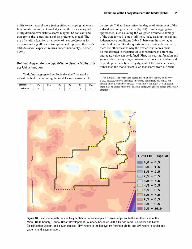
25
utility to each model score (using either a mapping table or a functional equation) acknowledges that the user’s marginal utility defined over criteria scores may not be constant and transforms the scores into a robust preference model. The use of a utility function as a model of user preferences for decision-making allows us to capture and represent the user’s attitudes about expected returns under uncertainty (Clemen, 1996).
Defining Aggregate Ecological-Value Using a Multiattrib-ute Utility Function
To define “aggregated ecological-value,” we need a robust method of combining the model scores (assumed to
Overview of the Ecosystem Portfolio Model (EPM)
be discrete10) that characterize the degree of attainment of the individual ecological criteria (fig. 18). Simple aggregation approaches, such as taking the weighted arithmetic average of the transformed scores (utilities), make assumptions about independence conditions (table 7) between the criteria, as described below. Besides questions of criteria independence, there are other reasons why the raw criteria scores must be transformed to measures of user preferences before any aggregate value can be defined. First, the scoring function and score scales for any single criterion are model-dependent and depend upon the subjective judgment of the model creators, rather than the model users, such that scores from different
Figure 16. Landscape patterns and fragmentation criterion applied to areas adjacent to the southern end of the Miami-Dade County, Florida, Urban Development Boundary, based on 2004-5 Florida Land-use, Cover and Forms Classification System land-cover classes. EPM refers to the Ecosystem Portfolio Model and LPF refers to landscape patterns and fragmentation.
parameter wBP wTES wRU wN wC wWF
value 1 1 2 4 4 4
10In the EPM, the criteria are scored based, at least in part, on discrete LULC classes, discrete distances (measured in numbers of 30m x 30 m pixels), and other attribute classes (for example, soil types), so, although there may be a large number of possible scores, the criteria scores are actually discrete.
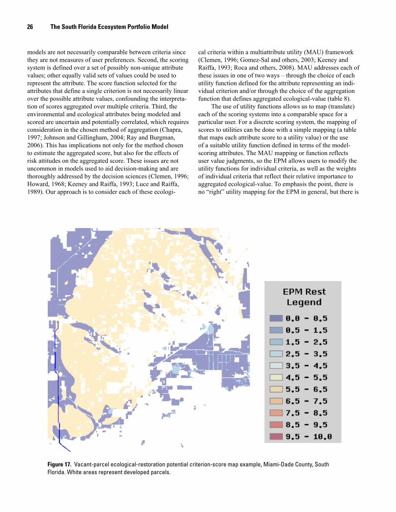
26 The South Florida Ecosystem Portfolio Model
models are not necessarily comparable between criteria since they are not measures of user preferences. Second, the scoring system is defined over a set of possibly non-unique attribute values; other equally valid sets of values could be used to represent the attribute. The score function selected for the attributes that define a single criterion is not necessarily linear over the possible attribute values, confounding the interpreta-tion of scores aggregated over multiple criteria. Third, the environmental and ecological attributes being modeled and scored are uncertain and potentially correlated, which requires consideration in the chosen method of aggregation (Chapra, 1997; Johnson and Gillingham, 2004; Ray and Burgman, 2006). This has implications not only for the method chosen to estimate the aggregated score, but also for the effects of risk attitudes on the aggregated score. These issues are not uncommon in models used to aid decision-making and are thoroughly addressed by the decision sciences (Clemen, 1996; Howard, 1968; Keeney and Raiffa, 1993; Luce and Raiffa, 1989). Our approach is to consider each of these ecologi-
cal criteria within a multiattribute utility (MAU) framework (Clemen, 1996; Gomez-Sal and others, 2003; Keeney and Raiffa, 1993; Roca and others, 2008). MAU addresses each of these issues in one of two ways – through the choice of each utility function defined for the attribute representing an indi-vidual criterion and/or through the choice of the aggregation function that defines aggregated ecological-value (table 8).
The use of utility functions allows us to map (translate) each of the scoring systems into a comparable space for a particular user. For a discrete scoring system, the mapping of scores to utilities can be done with a simple mapping (a table that maps each attribute score to a utility value) or the use of a suitable utility function defined in terms of the model-scoring attributes. The MAU mapping or function reflects user value judgments, so the EPM allows users to modify the utility functions for individual criteria, as well as the weights of individual criteria that reflect their relative importance to aggregated ecological-value. To emphasis the point, there is no “right” utility mapping for the EPM in general, but there is
Figure 17. Vacant-parcel ecological-restoration potential criterion-score map example, Miami-Dade County, South Florida. White areas represent developed parcels.
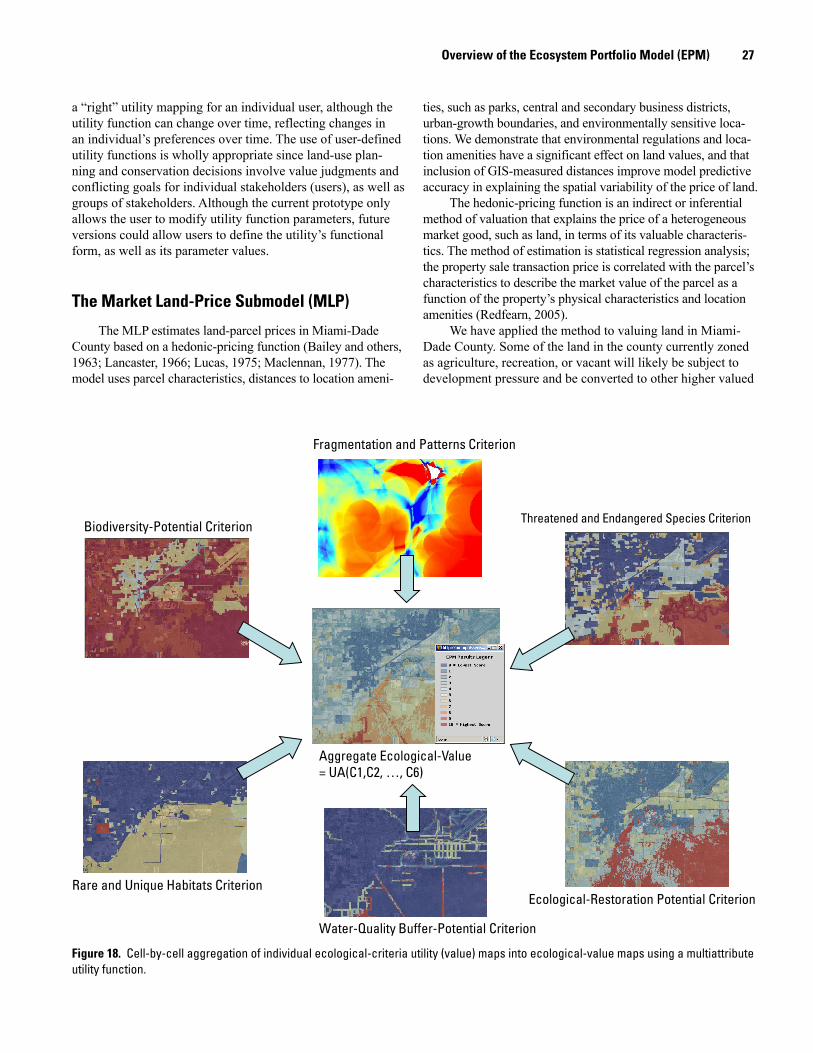
27 Overview of the Ecosystem Portfolio Model (EPM)
a “right” utility mapping for an individual user, although the utility function can change over time, reflecting changes in an individual’s preferences over time. The use of user-defined utility functions is wholly appropriate since land-use plan-ning and conservation decisions involve value judgments and conflicting goals for individual stakeholders (users), as well as groups of stakeholders. Although the current prototype only allows the user to modify utility function parameters, future versions could allow users to define the utility’s functional form, as well as its parameter values.
The Market Land-Price Submodel (MLP)
The MLP estimates land-parcel prices in Miami-Dade County based on a hedonic-pricing function (Bailey and others, 1963; Lancaster, 1966; Lucas, 1975; Maclennan, 1977). The model uses parcel characteristics, distances to location ameni-
ties, such as parks, central and secondary business districts, urban-growth boundaries, and environmentally sensitive loca-tions. We demonstrate that environmental regulations and loca-tion amenities have a significant effect on land values, and that inclusion of GIS-measured distances improve model predictive accuracy in explaining the spatial variability of the price of land.
The hedonic-pricing function is an indirect or inferential method of valuation that explains the price of a heterogeneous market good, such as land, in terms of its valuable characteris-tics. The method of estimation is statistical regression analysis; the property sale transaction price is correlated with the parcel’s characteristics to describe the market value of the parcel as a function of the property’s physical characteristics and location amenities (Redfearn, 2005).
We have applied the method to valuing land in Miami-Dade County. Some of the land in the county currently zoned as agriculture, recreation, or vacant will likely be subject to development pressure and be converted to other higher valued
Biodiversity-Potential CriterionThreatened and Endangered Species Criterion
Rare and Unique Habitats Criterion Ecological-Restoration Potential Criterion
Water-Quality Buffer-Potential Criterion
Fragmentation and Patterns Criterion
Aggregate Ecological-Value= UA(C1,C2, …, C6)
Figure 18. Cell-by-cell aggregation of individual ecological-criteria utility (value) maps into ecological-value maps using a multiattribute utility function.
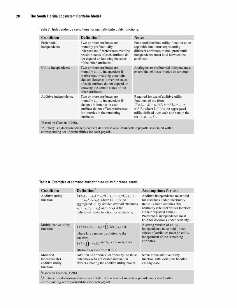
28 The South Florida Ecosystem Portfolio Model
Condition Definition1 Notes
Preferential independence
Two or more attributes are mutually preferentially independent if preferences over the possible states of each attribute do not depend on knowing the states of the other attributes.
For a multiattribute utility function to be separable into terms representing different attributes, mutual preferential independence must hold between the attributes.
Utility independence Two or more attributes are mutually utility independent if preferences involving uncertain choices (lotteries2) over the states of each attribute do not depend on knowing the certain states of the other attributes.
Analogous to preferential independence, except that choices involve uncertainty.
Additive independence Two or more attributes are mutually utility independent if changes in lotteries in each attribute do not affect preferences for lotteries in the remaining attributes.
Required for use of additive utility functions of the form: U(a,b,…,k) = wa*Ua + wb*Ub + … + wk*Ukutility defined over each attribute in the set {a, b, …, k}.
1Based on Clemen (1996). 2A lottery is a decision-sciences concept defined as a set of uncertain payoffs associated with a corresponding set of probabilities for each payoff.
Table 7. Independence conditions for multiattribute utility functions.
Condition Definition1 Assumptions for use
Additive utility function
U(x1,x2,…,xN) = w1*U1(x1) + w2*U2(x2) + … + wN*UN(xN)aggregated utility defined over all attributes xi {x1,x2,…,xN} and Ui(xi) is the individual utility function for attribute xi.
Additive independence must hold for decisions under uncertainty (table 7) and it assumes risk neutrality (the user values lotteries2 at their expected value). Preferential independence must hold for decisions under certainty.
Multiplicative utility function
where k is a nonzero solution to the equation:
and ki is the weight for
attribute i scaled from 0 to 1.
A strong version of utility independence must hold. Each subset of attributes must be utility-independent of the remaining attributes.
Modified (approximate) additive utility function
Addition of a “bonus” or “penalty” to those outcomes with noticeable interaction effects violating the additive utility model.
Same as the additive utility function with violations handled case-by-case.
1Based on Clemen (1996). 2A lottery is a decision-sciences concept defined as a set of uncertain payoffs associated with a corresponding set of probabilities for each payoff.
Table 8. Examples of common multiattribute utility functional forms.
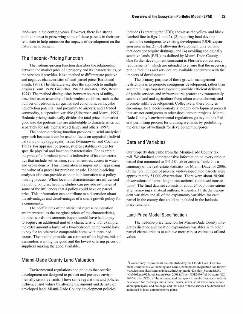
29 Overview of the Ecosystem Portfolio Model (EPM)
land-uses in the coming years. However, there is a strong public interest in preserving some of these parcels in their cur-rent state to help minimize the impacts of development on the natural environment.
The Hedonic-Pricing FunctionThe hedonic-pricing function describes the relationship
between the market price of a property and its characteristics, or the services it provides. It is a method to differentiate positive and negative characteristics of land-parcel price (Bartik and Smith, 1987). The literature ascribes the approach to multiple origins (Court, 1939; Grilliches, 1961; Lancaster, 1966; Rosen, 1974). The method distinguishes between sources of utility, described as an assembly of independent variables, such as the number of bedrooms, air quality, soil conditions, earthquake liquefaction potential, and proximity to airports, and a traded commodity, a dependent variable (Zilberman and Marra, 1993). Hedonic pricing statistically divides the total price of a market good into the portions that are attributable to characteristics not separately for sale themselves (Hanley and others, 1997).
The hedonic-pricing function provides a useful analytical approach because it can be used to focus on appraisal (individ-ual) and policy (aggregate) issues (Miranowski and Cochran, 1993). For appraisal purposes, studies establish values for specific physical and location characteristics. For example, the price of a farmland parcel is indicative of its characteris-tics that include soil erosion, rural amenities, access to water, and urban density. This information is important in appraising the value of a parcel for purchase or sale. Hedonic-pricing analyses also can provide economic information to a policy-making process. When location characteristics are influenced by public policies, hedonic studies can provide estimates of some of the influences that a policy could have on parcel price. This information can contribute to a discussion about the advantages and disadvantages of a smart growth policy for a community.
The coefficients of the statistical regression equation are interpreted as the marginal prices of the characteristics, in other words, the amounts buyers would have had to pay to acquire an additional unit of a characteristic. For example, the extra amount a buyer of a two-bedroom home would have to pay for an otherwise comparable home with three bed-rooms. The method provides an estimate of the highest bids of demanders wanting the good and the lowest offering prices of suppliers making the good available.
Miami-Dade County Land Valuation
Environmental regulations and policies that restrict development are designed to protect and preserve environ-mentally sensitive lands. These same regulations and policies influence land values by altering the amount and density of developed land. Miami-Dade County development policies
include (1) creating the UDB; shown as the yellow and black hatched line in figs. 1 and 2), (2) requiring land develop-ment to be contiguous to existing development (UDB expan-sion area in fig. 2), (3) allowing development only on land that does not require drainage, and (4) avoiding ecologically sensitive lands (EEL), as defined by Miami-Dade County. One further development constraint is Florida’s concurrency requirements11, which are intended to ensure that the necessary public facilities and services are available concurrent with the impacts of development.
The primary purpose of these growth-management restrictions is to promote contiguous development, rather than scattered, leap-frog development; provide efficient delivery of public services and infrastructure; protect environmentally sensitive land and agriculture from urban encroachment; and promote infill/redevelopment. Collectively, these policies encourage local decision-makers to deny development projects that are not contiguous to other development projects. Miami-Dade County’s environmental regulations go beyond the Fed-eral permitting process for draining wetlands by prohibiting the drainage of wetlands for development purposes.
Data and Variables
Our property data came from the Miami-Dade County tax roll. We obtained comprehensive information on every unique parcel that amounted to 541,184 observations. Table 9 is a summary of the real-estate statistics for Miami-Dade for 2006. Of the total number of parcels, undeveloped land parcels were approximately 51,000 observations. There were about 28,500 observations of “arms-length transactions” (unbiased transac-tions). The final data set consists of about 24,000 observations after removing statistical outliers. Appendix 3 lists the depen-dent variables and all of the explanatory variables for each parcel in the county that could be included in the hedonic-price function.
Land-Price Model Specification The hedonic-price function for Miami-Dade County inte-
grates distance and location explanatory variables with other parcel characteristics to achieve more robust estimates of land value.
11Concurrency requirements are established by the Florida Local Govern-ment Comprehensive Planning and Land Development Regulation Act (http://www.leg.state.fl.us/statutes/index.cfm?App_mode=Display_Statute&URL =Ch0163/part02.htm&StatuteYear=2008&Title=-%3E2008-%3EChapter%20163-%3EPart%20II). The act mandated that specific level-of-service standards be adopted for roadways, mass transit, water, sewer, solid waste, local recre-ation open space, and drainage, and that each of these services be defined and addressed in local comprehensive plans.
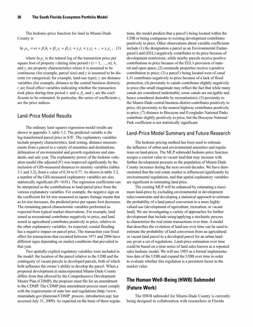
30 The South Florida Ecosystem Portfolio Model
The hedonic-price function for land in Miami-Dade County is
, (3)
where ln piτ is the natural log of the transaction price per square foot of property i during time period τ (τ = 1, …, n); hi and yi are property characteristics where h is assumed to be continuous (for example, parcel size) and y is assumed to be dis-crete (or categorical; for example, land-use type); zi are distance variables (for example, distance to the central business district); ti are fixed effect variables indicating whether the transaction took place during time period τ; and α, βj, and γi are the coef-ficients to be estimated. In particular, the series of coefficients γi are the price indices.
Land-Price Model Results
The ordinary least squares regression-model results are shown in appendix 3, table 3.2. The predicted variable is the log-transformed parcel price in $/ft2. The explanatory variables include property characteristics, land zoning, distance measure-ments from a parcel to a variety of amenities and destinations, delineation of environmental and growth regulations and stan-dards, and sale year. The explanatory power of the hedonic-valu-ation model (the adjusted R2) was improved significantly by the inclusion of GIS-measured distances to amenity variables (tables 3.1 and 3.2), from a value of 0.34 to 0.77. As shown in table 3.2, a number of the GIS-measured explanatory variables are also statistically significant (Pr <0.01). The regression coefficients can be interpreted as the contributions to land-parcel price from the various explanatory variables. For example, the negative sign on the coefficient for lot size measured as square footage means that as lot size increases, the predicted price per square foot decreases. The remaining parcel-characteristic variables performed as expected from typical market observations. For example, land zoned as recreational contributes negatively to price, and land zoned as agricultural contributes positively to price, relative to the other explanatory variables. As expected, coastal flooding has a negative impact on parcel price. The transaction year fixed effect for transactions that occurred between 1971 and 2006 have different signs depending on market conditions that prevailed in that year.
Two spatially-explicit regulatory variables were included in the model: the location of the parcel relative to the UDB and the continguity of vacant parcels to developed parcels, both of which both influence the owner’s ability to develop the parcel. When a proposed development in unincorporated Miami-Dade County differs from that allowed by the Comprehensive Development Master Plan (CDMP), the proposer must file for an amendment to the CDMP. The CDMP plan amendment process must comply with the requirements of state law and regulations (http://www.miamidade.gov/planzone/CDMP_process_introduction.asp; last accessed July 31, 2009). As expected on the basis of these regula-
tions, the model predicts that a parcel’s being located within the UDB or being contiguous to existing development contributes positively to price. Other observations about variable coefficients include (1) the designation a parcel as an Environmental Endan-gered Land (EEL) negatively contributes to its price because of development restrictions, while nearby parcels receive positive contributions to price because of the EEL’s provision of natu-ral and open space; (2) oceanside properties receive a positive contribution to price; (3) a parcel’s being located west of canal L31 contributes negatively to price because of a lack of flood protection; (4) proximity to canals contributes slightly negatively to price (the small magnitude may reflect the fact that while many canals are considered undesirable, some canals are navigable and hence considered desirable by recreationists); (5) proximity to the Miami-Dade central business district contributes positively to price; (6) proximity to the nearest highway contributes positively to price; (7) distance to Biscayne and Everglades National Parks contribute slightly positively to price, but the Biscayne National Park coefficient is not statistically significant.
Land-Price Model Summary and Future Research
The hedonic-pricing method has been used to estimate the influence of urban and environmental amenities and regula-tions on land-prices. The MLP submodel hedonic-price function assigns a current value to vacant land that may increase with further development pressure as the population of Miami-Dade County increases during the next several decades. We have dem-onstrated that the real estate market is influenced significantly by environmental regulations, and that spatial explanatory variables are significant in estimating land price.
The existing MLP will be enhanced by estimating a maxi-mum land-price by excluding environmental or development rules/constraints and developing a statistical approach to estimate the probability of a land parcel conversion to a more highly valued use (development of agriculture, recreation, or vacant land). We are investigating a variety of approaches for further development that include using/applying a stochastic process to characterize the real estate transactions over time. A model that describes the evolution of land-use over time can be used to estimate the probability of land conversion from an agricultural or vacant land parcel to a developed parcel for an urban land-use given a set of regulations. Land-price estimation over time could be based on a time series of land sales known as a repeated sales hedonic model. We will use 1985 as a formal implementa-tion date of the UDB and expand the UDB over time in order to evaluate whether this regulation is a persistent factor in the market value.
The Human Well-Being (HWB) Submodel (Future Work)
The HWB submodel for Miami-Dade County is currently being designed in collaboration with researchers at Florida
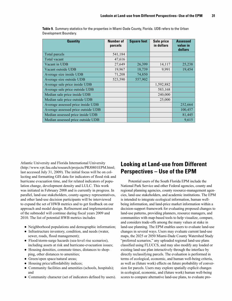
31
Atlantic University and Florida International University (http://www.vpt.fau.edu/research/projects/PRJ0801EPM.html; last accessed July 31, 2009). The initial focus will be on col-lecting and formatting GIS data for indicators of flood risk and hurricane evacuation time, and for related indicators of popu-lation change, development density and LULC. This work was initiated in February 2008 and is currently in progress. In parallel, land-use stakeholders, county-agency representatives, and other land-use decision participants will be interviewed to expand the set of HWB metrics and to get feedback on our approach and model design. Refinement and implementation of the submodel will continue during fiscal years 2009 and 2010. The list of potential HWB metrics includes
● Neighborhood populations and demographic information;● Infrastructure inventory, condition, and needs (water,
sewer, roads, flood management);● Flood/storm-surge hazards (sea-level rise scenarios),
including assets at risk and hurricane-evacuation issues;● Housing densities, commute times, distances to shop-
ping, other distances to amenities;● Green/open space/natural areas;● Housing price/affordability indices;● Community facilities and amenities (schools, hospitals);
and● Community character (set of indicators defined by users).
Looking at Land-use from Different Perspectives – Use of the EPM
Potential users of the South Florida EPM include the National Park Service and other Federal agencies, county and regional planning agencies, county resource-management agen-cies, land-use stakeholders, and academic institutions. The EPM is intended to integrate ecological information, human well-being information, and land-price market information within a decision-support framework for evaluating proposed changes to land-use patterns, providing planners, resource managers, and communities with map-based tools to help visualize, compare, and considers trade-offs among the many values at stake in land-use planning. The EPM enables users to evaluate land-use changes in several ways. Users may evaluate current land-use maps, the 2025 or 2050 Miami-Dade County Watershed Study “preferred scenarios,” any uploaded regional land-use plans classified using FLUCCS, and may also modify any loaded or existing land-use plan interactively through the interface by directly reclassifying parcels. The evaluation is performed in terms of ecological, economic, and human well-being criteria, as well as (future work) effects on future probability of conver-sion for parcels. Users may explore spatially explicit changes in ecological, economic, and (future work) human well-being scores to compare alternative land-use plans, to evaluate pro-
Lookoin at Land-use from Different Perspectives–Use of the EPM
Quantity Number of parcels
Square feet Sale pricein dollars
Assessed value in dollars
Total parcels 541,184Total vacant 47,616Vacant in UDB 27,649 26,399 14,117 25,238Vacant outside UDB 19,967 18,739 9,991 19,454Average size inside UDB 71,208 74,850Average size outside UDB 523,590 557,902Average sale price inside UDB 1,592,882Average sale price outside UDB 583,168Median sale price inside UDB 240,000Median sale price outside UDB 25,000Average assessed price inside UDB 252,664Average assessed price outside UDB 100,457Median assessed price inside UDB 81,445Median assessed price outside UDB 9,615
Table 9. Summary statistics for the properties in Miami-Dade County, Florida. UDB refers to the Urban Development Boundary.
32 The South Florida Ecosystem Portfolio Model
posed developments, to evaluate historical trends in land-use changes, and to evaluate simulated/projected future land-use changes. The criteria, metrics, and models used for the EVM were chosen in collaboration with potential users, the same process that will be used for choosing the criteria for the HWB. The MLP is based on real estate market transaction data, parcel characteristic data, and other relevant data. Each of the EPM submodels were designed and implemented with the goal of finding an acceptable compromise between several compet-ing objectives for evaluating land-use plans (1) credibility, (2) transparency, (3) flexibility, and (4) ease of use.
Our intent is to enable users to think about natural values related to land-use planning and decision-making in several ways (by using the three submodels) and to explore in more detail the criteria and metrics of each submodel. The EPM currently makes no attempt to aggregate ecological-value, land-price, and human well-being metrics into a single mea-sure of value, although this synthesis will be explored in future work. However, the purpose of the EPM is not to identify a single index to determine the best land-use plan among a list of alternative plans, for two reasons. First, we treat land-use plan-ning as a participatory process involving parties with different preferences among conflicting goals. Second, land-use plans are inherently heterogeneous, so no one plan is better than every other consistently throughout the map, and in land-use planning this heterogeneity matters to participants. Thus, the EPM is a map-based multicriteria evaluation tool that stakeholders can use to debate tradeoffs at multiple scales within a participatory process. The EPM is intended to help inform the debate, not to support a particular position.
References Cited Adamus, C.L., and Bergman, M.J., 1995, Estimating nonpoint
source pollution loads with a GIS screening model: Water Resources Bulletin, v. 31, no. 4, p. 647-655.
Bailey, M.J., Muth, R.F., and Nourse, H.O., 1963, A regression method for real estate price index construction: Journal of the American Statistical Association, v. 58, p. 933-942.
Banzhaf, S., and Boyd, J., 2005, The architecture and measurement of an ecosystem services index: Resources for the Future, RFF DP 05-22, 54 p.
Bartik, T., and Smith, V.K., 1987, Urban amenities and public policy, in Mills, E., ed., Handbook of regional and urban economics: Amsterdam, Elsevier Science Publishers B.V., p. 1207-1254.
Blair, R.B., 1996, Land use and avian species diversity along an urban gradient: Ecological Applications, v. 6, no. 2, p. 506-519.
Blake, N.B., 1980, Land into water, water into land - a history of water management in south Florida: Gainesville, FL, University Presses of Florida.
Boyd, J., and Wainger, L., 2003, Measuring ecosystem service benefits—the use of landscape analysis to evaluate
environmental trades and compensation: Resources for the Future, Discussion Paper 02-63, 130 p.
Brody, S.D., 2008, Ecosystem planning in Florida - solving regional problems through local decision-making: Burlington, VT, Ashgate, 212 p.
Cantillo, A.Y., Hale, K., Collins, E., Pikula, L., and Caballero, R., 2000, Biscayne bay—environmental history and annotated bibliography: National Oceanic and Atmospheric Administration, NOAA Technical Memorandum NOS NCCOS CCMA 145, 116 p.
Chapman, A.E., 1991, History of south Florida, in Boswell, T.D., ed., South Florida - winds of change: Coral Gables, FL, University of Miami, p. 31-42.
Chapra, S.C., 1997, Surface water-quality modeling: New York, McGraw-Hill, 844 p.
Clemen, R.T., 1996, Making hard decisions—an introduction to decision analysis: Pacific Grove, CA, Duxbury Press, 664 p.
Costanza, R., Cumberland, J., Daly, H., Goodland, R., and Norgaard, R., 1997, An introduction to ecological economics: Boca Raton, FL, St. Lucie Press, 275 p.
Costanza, R., and Folke, C., 1997, Valuing ecosystem services with efficiency, fairness, and sustainability as goals, in Daily, G., ed., Nature’s services—societal dependence on natural ecosystems: Washington, D.C., Island Press, p. 49-68.
Court, A., 1939, Hedonic price indexes with automotive examples, The dynamics of automobile demand: New York, General Motors Corporation, p. 99-117.
Daily, G.C., ed., 1997, Nature’s services—societal dependence on natural ecosystems: Washington, D.C., Island Press, 392 p.
Davis, S.M., Ogden, J.C., and Park, W.A., 1994, Everglades - the ecosystem and its restoration: Delray Beach, FL, St. Lucie Press, 826 p.
Edwards, W., 1977, How to use multiattribute utility measurement for social decisionmaking: IEEE Transactions on Systems, Man, and Cybernetics, v. SMC-7, no. 5, p. 326-340.
Edwards, W., and Hutton, B.F., 1994, SMARTS and SMARTER —improved simple methods for multiattribute utility measurement: Organizational Behavior and Human Decision Processes, v. 60, no. 3, p. 306-325.
Eppink, F.V., van den Bergh, J.C.J.M., and Rietveld, P., 2004, Modeling biodiversity and land use—urban growth, agriculture, and nature in a wetland area: Ecological Economics, v. 51, p. 201-216.
Figge, F., 2004, Biofolio—applying portfolio theory to biodiversity: Biodiversity and Conservation, v. 13, no. 827-849.
Foster, J., 1997, Valuing nature—ethics, economics and the environment: New York, Routledge, 273 p.
Goldstein, J.H., 1994, The impact of Federal programs on wetlands, v. 2: Washington, D.C., U.S. Department of the Interior [Available online at http://www.doi.gov/oepc/wetlands2/v2ch19.html#refs, last accessed July 30, 2009].
33
Gomez-Sal, A., Belmontes, J.-A., and Nicolau, J.-M., 2003, Assessing landscape values - a proposal for a multidimensional conceptual model: Ecological Modelling, v. 168, p. 319-341.
Goodland, R., and Daly, H., 1995, Environmental sustainability, in Vanclay, F., and Bronstein, D.A., eds., Environmental and social impact assessment: New York, Wiley, p. 303-322.
Goodstein, E.S., 2002, Economics and the environment: New York, John Wiley & Sons, Inc., 545 p.
Goulder, L.H., and Kennedy, D., 1997, Valuing ecosystem services - philosophical bases and empirical methods, in Daily, G., ed., Nature’s services—societal dependence on natural ecosystems: Washington, D.C., Island Press, p. 23-47.
Gregory, R., 1999, Identifying environmental values, in Dale, V., and English, M., eds., Tools to aid environmental decision making: New York, Spring-Verlag, p. 33-58.
Grilliches, Z., 1961, Hedonic price indexes for automobiles: An econometric analysis of quality change: National Bureau of Economic Research, 137-196 p.
Groot, R., 2006, Function-analysis and valuation as a tool to assess land use conflicts in planning for sustainable, multi-functional landscapes: Landscape and Urban Planning, v. 75, p. 175-186.
Grunwald, M., 2006, The swamp—the everglades, Florida, and the politics of paradise: New York, Simon & Schuster, 450 p.
Hanley, N., Shogren, J., and White, B., 1997, Environmental economics in theory and practice: New York, Oxford University Press, 464 p.
Harwell, C.C., Deren, C.W., Snyder, G.H., Solecki, W.D., Wilson, J., and Harwell, M.A., 1999a, Use of a conceptual model of societal drivers of ecological change in south Florida—implications of an ecosystem management scenario: Urban Ecosystems, v. 3, p. 345-368.
Harwell, M.A., 1997, Ecosystem management of south Florida: BioScience, v. 47, no. 8, p. 499-512.
Harwell, M.A., Gentile, J.H., Bartuska, A., Harwell, C.C., Myers, V., Obeysekera, J., Ogden, J.C., and Tosini, S.C., 1999b, A science-based strategy for ecological restoration in south Florida: Urban Ecosystems, v. 3, p. 201-222.
Hassan, R.M., Scholes, R., and Ash, N., 2005, Ecosystems and human well-being - current state and trends—findings of the Condition and Trends Working Group of the Millennium Ecosystem Assessment: Washington, DC, Island Press, v. 1, 917 p.
Heal, G., 2000, Nature and the marketplace—capturing the value of ecosystem services: Washington, D.C., Island Press, 203 p.
Hildebrand, S.G., and Cannon, J.B., 1993, Environmental analysis - the nepa experience: Ann Arbor, MI, Lewis Publishers, 763 p.
Howard, R.A., 1968, The foundations of decision analysis: IEEE Transactions on Systems, Science and Cybernetics, v. SSC-4, no. 3, p. 211-219.
Johnson, C.J., and Gillingham, M.P., 2004, Mapping uncertainty: Sensitivity of wildlife habitat rankings to expert opinion: Journal of Applied Ecology, v. 41, p. 1032-1041.
Kambly, S., and Moreland, T.R., 2009, Land cover trends in the southern Florida coastal plain: U.S. Geological Survey Scientific Investigations Report 2009–5054, 16 p.
Keeney, R.L., and Raiffa, H., 1993, Decisions with multiple objectives—preferences and value tradeoffs: New York, Cambridge University Press, 569 p.
Lancaster, K.J., 1966, A new approach to consumer theory: Journal of Political Economy, v. 74, p. 132-157.
Lucas, R.E.B., 1975, Hedonic price functions: Economic Inquiry, v. 13, p. 157-178.
Luce, R.D., and Raiffa, H., 1989, Games and decisions - introduction and critical survey: New York, Dover Publications, 509 p.
Maclennan, D., 1977, Some thoughts on the nature and purpose of hedonic price functions: Urban Studies, v. 14, p. 59-71.
Marella, R.L., 1992, Factors that affect public-supply water use in Florida, with a section on projected water use to the year 2020: U.S. Geological Survey, Water-Resources Investigations Report 99-4002, 88 p.
Marsh, L.L., and Lallas, P.L., 1995, Focused, special-area conservation planning—an approach to reconciling development and environmental protection, in Porter, D.R., and Salvesen, D.A., eds., Collaborative planning for wetlands and wildlife: Issues and examples: Washington, D.C., Island Press, p. 7–34.
McGarigal, K., and Marks, B., 1995, FRAGSTATS—spatial pattern analysis program for quantifying landscape structure: U.S. Department of Agriculture, Forest Service, Pacific Northwest Research Station, General Technical Report PNW-GTR-351, 122 p.
Miami-Dade County Department of Planning & Zoning, 2008, Population projections—components of change: Miami, FL, Miami-Dade County Department of Planning & Zoning.
Millennium Ecosystem Assessment, 2003, Ecosystems and human well-being—a framework for assessment: Washington, D.C., Island Press, 245 p.
Miranowski, J., and Cochran, M., 1993, Economics of land in agriculture, in Carlson, G., Zilberman, D., and Miranowski, J., eds., Agricultural and environmental resource economics, p. 392-440.
Morris, P., and Therivel, R., 2009, Methods of environmental impact assessment (3rd ed.): New York, Routledge, 560 p. National Research Council, 1994, Assigning economic value to natural resources: Washington, D.C., National Academy Press, 185 p.
National Research Council, 1994, Assigning economic value to natural resources: Washington, D.C., National Academy Press, 185 p.
National Research Council, 2005, Evaluating ecological tradeoffs: Washington, D.C., National Academy Press, 7 p.
National Research Council, 2007, Progress toward
References Cited
34 The South Florida Ecosystem Portfolio Model
restoring the everglades—the first biennial review, 2006: Washington, D.C., National Academy Press, 235 p.
Peck, S., 1998, Planning for biodiversity—issues and examples: Washington, D.C., Island Press, 221 p.
Percival, R.V., Miller, A.S., Leape, J.P., and Schroeder, C.H., 2006, Environmental regulation : Law, science, and policy (5th ed.): New York, Aspen Publishers, 1202 p.
Pritchard, L., Jr., Folke, C., and Gunderson, L., 2000, Valuation of ecosystem services in institutional context:
Ecosystems, v. 3, p. 36-40.Rabin, C., and Pinzur, M.I., 2008, Alvarez vetoes growth plan
in west Miami-Dade, Miami Herald: Miami, FL, [available online at http://www.miamiherald.com, last accessed July 25, 2008].
Randolph, J., 2004, Environmental land use planning and management: Washington, D.C., Island Press, 664 p.
Ray, N., and Burgman, M.A., 2006, Subjective uncertainties in habitat suitability maps: Ecological Modelling, v. 195, p. 172-186.
Renken, R.A., Dixon, J., Koehmstedt, J., Ishman, S., Lietiz, A.C., Marella, R.L., Telis, P., Rogers, J., and Memberg, S., 2005, Impact of anthropogenic development on coastal ground-water hydrology in southeastern Florida, 1900-2000, U.S. Geological Survey Circular 1275, 77 p.
Roca, E., Gamboa, G., and Tabara, J.D., 2008, Assessing the multidimensionality of coastal erosion risks—public participation and multicriteria analysis in a mediterranean coastal system: Risk Analysis, v. 28, no. 2, p. 399-411.
Rosen, S., 1974, Hedonic prices and implicit markets: Product differentiation in pure competition: Journal of Political Economy, v. 82, p. 34-55.
Solecki, W.D., Long, J., Harwell, C.C., Myers, V., and Zubrow, E., 1999, Human-environment interactions in south florida’s everglades region—systems of ecological
degradation and restoration: Urban Ecosystems, v. 3, p. 305-343.
South Florida Regional Planning Council, 2003, Guide for developments of regional impact: South Florida Regional Planning Council [available online at http://www.sfrpc.com/dri/guide.htm, last accessed July 30, 2009].
South Florida Regional Planning Council, 2004, Strategic regional policy plan for south Florida: South Florida Regional Planning Council, 100 p.
Spellerberg, I.F., 1998, Ecological effects of roads and traffic: A literature review: Global Ecology and Biogeography Letters, v. 7, p. 317-333.
Tischendorf, L., 2001, Can landscape indices predict ecological processes consistently?: Landscape Ecology, v. 16, p. 235-254.
U.S. Geological Survey, 2007, Facing tomorrow’s challenges —U.S. Geological Survey science in the decade 2007–2017: U.S. Geological Survey Circular 1309, 70 p.
Wilson, M.A., and Carpenter, S.R., 1999, Economic valuation of freshwater ecosystem services in the United States —1971-1997: Ecological Applications, v. 9, no. 3, p. 772-783.
Wilson, M.A., and Howarth, R.B., 2002, Discourse-based valuation of ecosystem services—establishing fair outcomes through group deliberation: Ecological Economics, v. 41, p. 431-443.
Zilberman, D., and Marra, M., 1993, Agricultural externalities, in Carlson, G., Zilberman, D., and Miranowski, J., eds., Agricultural and environmental resource economics: New York, Oxford University Press, p. 221-267.
Zwick, P.D., and Carr, M.H., 2006, Florida 2060—a population distribution scenario for the state of Florida: University of Florida Geoplan Center, 25 p.

35
Appendixes 1–3

36 The South Florida Ecosystem Portfolio Model
This page intentionally left blank
37
Appendix 1. GAP-Model Scoring Tables for FLUCCS Codes and Species Used in the EPM for the Biodiversity-Potential Ecological-Value Criterion
GAP scoring table for mammals (link to fluccs_mammals.xls.zip)
GAP scoring table for birds (link to fluccs_birds.xls.zip)
GAP scoring table for reptiles and amphibians (link to fluccs_herps.xls.zip)
Appendix 2. GAP-Model Scoring Tables for FLUCCS codes and Species Used in the EPM for the Threatened and Endangered Species Ecological-Value Crite-rion (U.S. Fish and Wildlife Service Multispecies Recovery Plan)
The list of species used in this criterion is based on the U.S. Fish and Wildlife Service Multispecies Recovery Plan (MSRP) (http://www.fws.gov/verobeach/index.cfm?Method=programs&NavProgramCategoryID=3&programID=107&ProgramCategoryID=3)
GAP scoring table for MSRP species (link to fluccs_msrp.xls.zip)
Appendix
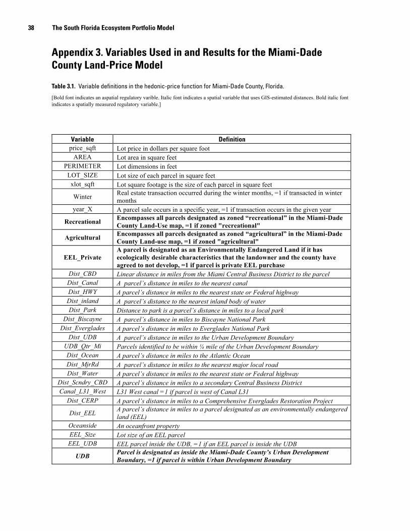
38 The South Florida Ecosystem Portfolio Model
Appendix 3. Variables Used in and Results for the Miami-Dade County Land-Price Model
Table 3.1. Variable definitions in the hedonic-price function for Miami-Dade County, Florida.
[Bold font indicates an aspatial regulatory varible. Italic font indicates a spatial variable that uses GIS-estimated distances. Bold italic font indicates a spatially measured regulatory variable.]
Variable Definitionprice_sqft Lot price in dollars per square foot
AREA Lot area in square feetPERIMETER Lot dimensions in feet
LOT_SIZE Lot size of each parcel in square feetxlot_sqft Lot square footage is the size of each parcel in square feet
Winter Real estate transaction occurred during the winter months, =1 if transacted in winter months
year_X A parcel sale occurs in a specific year, =1 if transaction occurs in the given year
Recreational Encompasses all parcels designated as zoned “recreational” in the Miami-Dade County Land-Use map, =1 if zoned "recreational"
Agricultural Encompasses all parcels designated as zoned “agricultural” in the Miami-Dade County Land-use map, =1 if zoned "agricultural"
EEL_PrivateA parcel is designated as an Environmentally Endangered Land if it has ecologically desirable characteristics that the landowner and the county have agreed to not develop, =1 if parcel is private EEL purchase
Dist_CBD Linear distance in miles from the Miami Central Business District to the parcelDist_Canal A parcel’s distance in miles to the nearest canalDist_HWY A parcel’s distance in miles to the nearest state or Federal highway Dist_inland A parcel’s distance to the nearest inland body of water Dist_Park Distance to park is a parcel’s distance in miles to a local park
Dist_Biscayne A parcel’s distance in miles to Biscayne National ParkDist_Everglades A parcel’s distance in miles to Everglades National Park
Dist_UDB A parcel’s distance in miles to the Urban Development BoundaryUDB_Qtr_Mi Parcels identified to be within mile of the Urban Development BoundaryDist_Ocean A parcel’s distance in miles to the Atlantic OceanDist_MjrRd A parcel’s distance in miles to the nearest major local roadDist_Water A parcel’s distance in miles to the nearest state or Federal highway
Dist_Scndry_CBD A parcel’s distance in miles to a secondary Central Business DistrictCanal_L31_West L31 West canal =1 if parcel is west of Canal L31
Dist_CERP A parcel’s distance in miles to a Comprehensive Everglades Restoration Project
Dist_EEL A parcel’s distance in miles to a parcel designated as an environmentally endangered land (EEL)
Oceanside An oceanfront propertyEEL_Size Lot size of an EEL parcelEEL_UDB EEL parcel inside the UDB, =1 if an EEL parcel is inside the UDB
UDB Parcel is designated as inside the Miami-Dade County’s Urban Development Boundary, =1 if parcel is within Urban Development Boundary
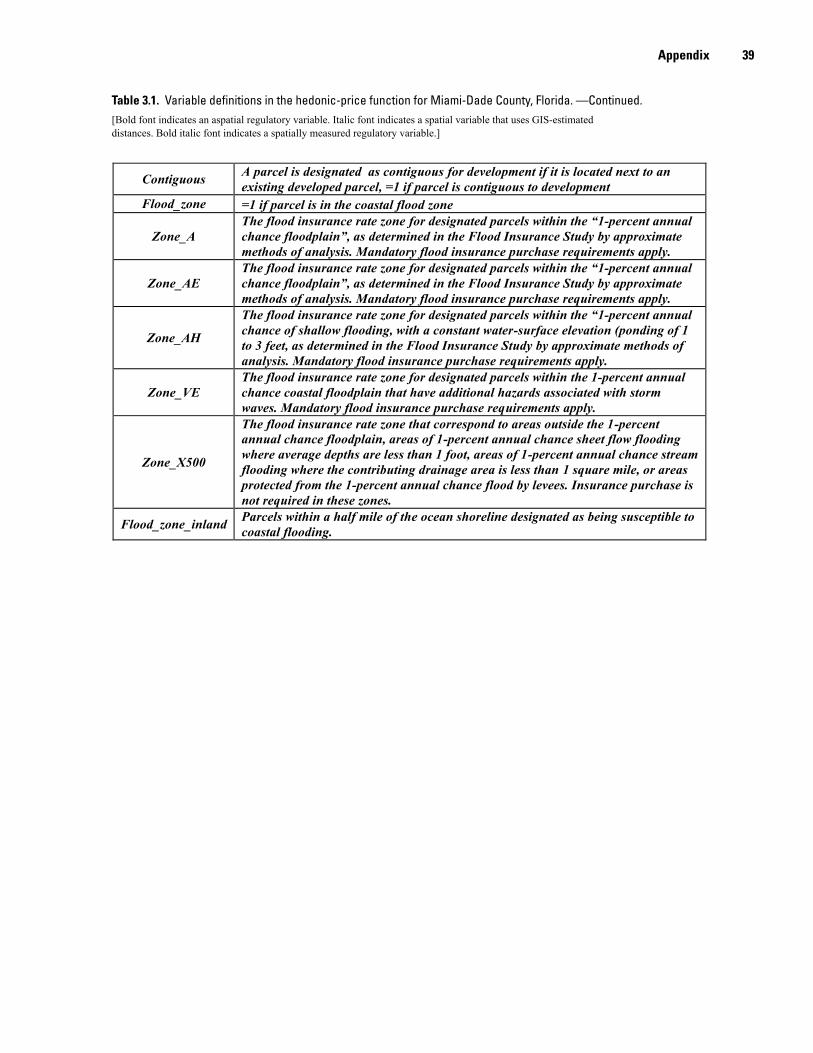
39
Table 3.1. Variable definitions in the hedonic-price function for Miami-Dade County, Florida. —Continued. [Bold font indicates an aspatial regulatory variable. Italic font indicates a spatial variable that uses GIS-estimated distances. Bold italic font indicates a spatially measured regulatory variable.]
Contiguous A parcel is designated as contiguous for development if it is located next to an existing developed parcel, =1 if parcel is contiguous to development
Flood_zone =1 if parcel is in the coastal flood zone
Zone_AThe flood insurance rate zone for designated parcels within the “1-percent annual chance floodplain”, as determined in the Flood Insurance Study by approximate methods of analysis. Mandatory flood insurance purchase requirements apply.
Zone_AEThe flood insurance rate zone for designated parcels within the “1-percent annual chance floodplain”, as determined in the Flood Insurance Study by approximate methods of analysis. Mandatory flood insurance purchase requirements apply.
Zone_AH
The flood insurance rate zone for designated parcels within the “1-percent annual chance of shallow flooding, with a constant water-surface elevation (ponding of 1 to 3 feet, as determined in the Flood Insurance Study by approximate methods of analysis. Mandatory flood insurance purchase requirements apply.
Zone_VEThe flood insurance rate zone for designated parcels within the 1-percent annual chance coastal floodplain that have additional hazards associated with storm waves. Mandatory flood insurance purchase requirements apply.
Zone_X500
The flood insurance rate zone that correspond to areas outside the 1-percent annual chance floodplain, areas of 1-percent annual chance sheet flow flooding where average depths are less than 1 foot, areas of 1-percent annual chance stream flooding where the contributing drainage area is less than 1 square mile, or areas protected from the 1-percent annual chance flood by levees. Insurance purchase is not required in these zones.
Flood_zone_inland Parcels within a half mile of the ocean shoreline designated as being susceptible to coastal flooding.
Appendix
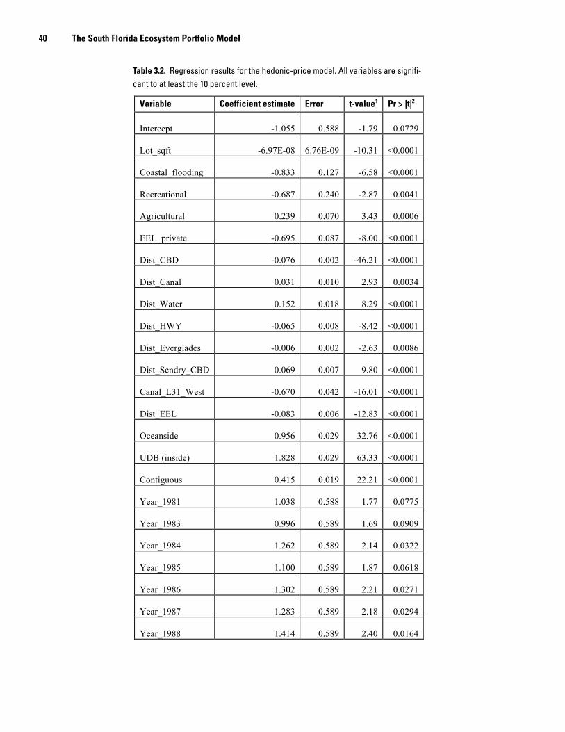
40 The South Florida Ecosystem Portfolio Model
Table 3.2. Regression results for the hedonic-price model. All variables are signifi-cant to at least the 10 percent level.
Variable Coefficient estimate Error t-value1 Pr > |t|2
Intercept -1.055 0.588 -1.79 0.0729
Lot_sqft -6.97E-08 6.76E-09 -10.31 <0.0001
Coastal_flooding -0.833 0.127 -6.58 <0.0001
Recreational -0.687 0.240 -2.87 0.0041
Agricultural 0.239 0.070 3.43 0.0006
EEL_private -0.695 0.087 -8.00 <0.0001
Dist_CBD -0.076 0.002 -46.21 <0.0001
Dist_Canal 0.031 0.010 2.93 0.0034
Dist_Water 0.152 0.018 8.29 <0.0001
Dist_HWY -0.065 0.008 -8.42 <0.0001
Dist_Everglades -0.006 0.002 -2.63 0.0086
Dist_Scndry_CBD 0.069 0.007 9.80 <0.0001
Canal_L31_West -0.670 0.042 -16.01 <0.0001
Dist_EEL -0.083 0.006 -12.83 <0.0001
Oceanside 0.956 0.029 32.76 <0.0001
UDB (inside) 1.828 0.029 63.33 <0.0001
Contiguous 0.415 0.019 22.21 <0.0001
Year_1981 1.038 0.588 1.77 0.0775
Year_1983 0.996 0.589 1.69 0.0909
Year_1984 1.262 0.589 2.14 0.0322
Year_1985 1.100 0.589 1.87 0.0618
Year_1986 1.302 0.589 2.21 0.0271
Year_1987 1.283 0.589 2.18 0.0294
Year_1988 1.414 0.589 2.40 0.0164
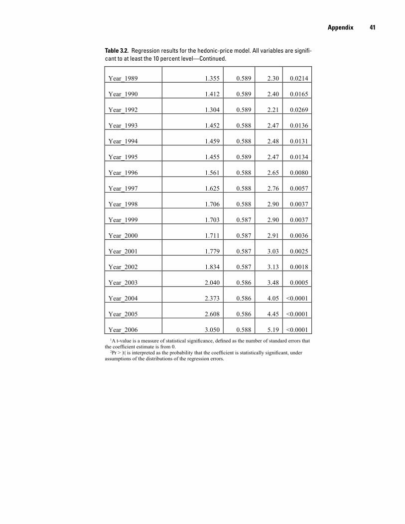
41
Table 3.2. Regression results for the hedonic-price model. All variables are signifi-cant to at least the 10 percent level—Continued.
1A t-value is a measure of statistical significance, defined as the number of standard errors that the coefficient estimate is from 0.
2Pr > |t| is interpreted as the probability that the coefficient is statistically significant, under assumptions of the distributions of the regression errors.
Year_1989 1.355 0.589 2.30 0.0214
Year_1990 1.412 0.589 2.40 0.0165
Year_1992 1.304 0.589 2.21 0.0269
Year_1993 1.452 0.588 2.47 0.0136
Year_1994 1.459 0.588 2.48 0.0131
Year_1995 1.455 0.589 2.47 0.0134
Year_1996 1.561 0.588 2.65 0.0080
Year_1997 1.625 0.588 2.76 0.0057
Year_1998 1.706 0.588 2.90 0.0037
Year_1999 1.703 0.587 2.90 0.0037
Year_2000 1.711 0.587 2.91 0.0036
Year_2001 1.779 0.587 3.03 0.0025
Year_2002 1.834 0.587 3.13 0.0018
Year_2003 2.040 0.586 3.48 0.0005
Year_2004 2.373 0.586 4.05 <0.0001
Year_2005 2.608 0.586 4.45 <0.0001
Year_2006 3.050 0.588 5.19 <0.0001
Appendix

Produced in the Western Region, Menlo Park, CaliforniaManuscript approved for publication, August 6, 2009Text edited by Tracey SuzukiLayout and design by Stephen L. Scott

Labiosa and others—The South Florida Ecosystem
Portfolio Model—
Scientific Investigations Report 2009-5181