The Solution of Unconfined Seepage Problem Using Natural Element Method (NEM) Coupled With Genetic Algorithm (GA)

Applied Mathematical Modelling 37 (2013) 2775–2786

Contents lists available at SciVerse ScienceDirect

Applied Mathematical Modelling

journal homepage: www.elsevier .com/locate /apm

The solution of unconfined seepage problem using Natural ElementMethod (NEM) coupled with Genetic Algorithm (GA)

Sh. Shahrokhabadi a,⇑, M.M. Toufigh b

a Civil Engineering Department, Vali-e-Asr University of Rafsanjan, 22 Bahman Squ., Rafsanjan, Iranb Civil Engineering Department, Shahid Bahonar University of Kerman, 22 Bahman Blv., Kerman, Iran

a r t i c l e i n f o a b s t r a c t

Article history:Received 6 June 2011Received in revised form 28 May 2012Accepted 4 June 2012Available online 16 June 2012

Keywords:Natural Element MethodGenetic AlgorithmSeepageMesh-free

0307-904X/$ - see front matter � 2012 Elsevier Inchttp://dx.doi.org/10.1016/j.apm.2012.06.030

⇑ Corresponding author. Tel.: +98 913 291 5015;E-mail address: [email protected] (S

Phreatic line detection is a major challenge in seepage problems which should be solved byiterative solving procedures. In conventional methods such as finite element method(FEM), an updating mesh is needed in each iteration where the qualities of the mesh andthe nodal connectivity have significant impact on the results. The main aim of this studyis to use a method not to be sensitive to mesh generation.

In this study, to obtain the optimal phreatic line by the 4th degree polynomial, NaturalElement Method (NEM) and Genetic Algorithm (GA) are implemented. Based on the energyprinciple, an objective function is defined to control the phreatic line position. In theoptimization procedure, NEM is utilized to analyze the problem. NEM is a domain typemesh-free method, adapted to geometry of the problem in each iteration. Results displaymore convergence and flexibility of the present method in comparison with previousstudies.

� 2012 Elsevier Inc. All rights reserved.

1. Introduction

The position of the phreatic line in earth dams cannot be determined easily. Thus, phreatic line detection has been studiedby many researchers as a significant issue [1–4]. In general, Prediction of seepage flow in earth dams is studied throughanalytical, numerical, and recently artificial intelligence methods based on observational statistical data [5]. When statisticsare not available, as in preconstruction state, there are two distinct methods, analytical and numerical, to deal with uncon-fined seepage problems.

New researches show brilliant achievements in the field of analytical solutions [6], however, these methods are not appli-cable in solving complex geometries, inhomogeneous, and anisotropic problems. Moreover, numerical methods are widelyused to simulate complex geometries; or inhomogeneous problems [7–10]. Finite element method (FEM) and finite differ-ence method (FDM) are conventionally exploited to solve the seepage problems. Since the position of phreatic line is notpredictable in advance, the unconfined seepage problem requires an iterative process to locate the free surface.

In FEM, fixed mesh and adaptive mesh are used to detect the phreatic line. In the adaptive mesh methods, the domain ofthe problem is needed to be re-meshed at each step of iteration. This may increase the computational costs and may lead tomesh distortion and non-convergence [11]. Therefore, most of studies are accomplished in the form of fixed mesh methods.In the fixed mesh methods, element permeability decreases iteratively and finally results in the separation of unsaturatedand saturated zone [12].

. All rights reserved.

fax: +98 341 245 8597.h. Shahrokhabadi).

http://dx.doi.org/10.1016/j.apm.2012.06.030

mailto:[email protected]

http://dx.doi.org/10.1016/j.apm.2012.06.030

http://www.sciencedirect.com/science/journal/0307904X

http://www.elsevier.com/locate/apm

2776 Sh. Shahrokhabadi, M.M. Toufigh / Applied Mathematical Modelling 37 (2013) 2775–2786

Due to the fact that permeability changes, the problem should be resolved non-linearly. The seepage problem domain isdivided into three parts: saturation, unsaturation and transition zones. In the transition zone, the permeability is a functionof pore pressure [13]. Consequently, the elements, crossed by the free surface, are singled out and defined as transitionalelements. Recently, manifold elements are used in fixed mesh methods and since the shape of manifold elements can bearbitrary, one does not need to change the permeability of transitional elements. Moreover, the tetrahedral finite elementmeshes are chosen as the mathematical meshes covering the whole dam body to solve unconfined seepage in 3D problems.During the process of iteration for locating the free surface, the tetrahedral meshes remain unchanged, and only the mediumin the seepage domain is taken into consideration [11].

Mesh adaptation is a linear and simple approach which is used in the finite element method [14], but this method islimited to a new mesh generation in each step of iteration. Thus, it requires more computational time and may even leadto distorted meshes. In addition, mesh distortion may cause non-convergence conditions [11]. Moreover, using mesh adap-tation results in non-tangency of the phreatic line with the downstream slope that is incompatible with the flow continuity.Coupling adaptive mesh with Nelder–Mead optimization is a way to overcome this difficulty [12]. Although the phreatic lineis forced to be tangential on the downstream slope, mesh distortion remains as a critical problem in this approach. Therefore,selecting a method that is not sensitive to mesh generation is a fundamental step in adaptive mesh procedure.

In recent decades, development of mesh-free methods which are used in advanced analysis of problems with floatinggeometry; seems to be an alternative remedy to solve problems [15–19]. In general, mesh-free methods are divided intotwo categories: boundary type and domain type methods [20]. In both of them, Radial Basis Function (RBF) is the basicconcept to approximate the results [21,22]. Local Radial Basis function-based on differential quadrature method (RBF-DQ)is a domain type mesh-free method which is recently used in seepage analysis [23]. The radius of supporting domain, how-ever, is constant for all of the nodes and it needs special consideration along the boundaries.

Furthermore, in the domain type of mesh-free methods a large number of nodes are required because each single RBFdoes not satisfy the governing equation and also, these methods are sensitive to nodes position [20,24–28]. Method offundamental solution is considered as another alternative in mesh-free methods which is a boundary type method, butthe flow continuity is not considered in the solution procedure and it is not applicable in inhomogeneous domains [29].

The aim of this study is to introduce a method which is classified in adaptive mesh procedures, in which mesh distortionis not a critical issue. In each step of iteration, the problem geometry changes, so the position of the nodes update in eachstep. Therefore, Natural Element Method (NEM) is a mesh-free method that can meet this requirement without concernabout the nodes position or radius of support domain. NEM is a local compact support method and possesses delta kroneker,which would lead to the simplicity usage of the method [30]. The NEM and Genetic Algorithm (GA) are used simultaneouslyto adjust a 4th degree polynomial for phreatic line based on solving unconfined seepage problem. The achieved flow pathshould satisfy the requirements of the energy principle and the flow continuity.

2. Governing equations and boundary conditions

Seepage problems can be considered in both steady-state and unsteady cases. In this study, laminar steady-state flow isconsidered and the problem domain is fully saturated. In order for interested readers to study more about unsteady case,they are referred to advanced soil mechanics [31].

Seepage flow through an element is:

q ¼ �krðTHÞA; ð1Þ

where q is discharge vector, k is soil permeability, rðTHÞ is total head gradient, and A is the area of soil element.Total head at every given node is defined by energy principle:

TH ¼ EH þ PH; ð2Þ

where TH is total head, EH is node elevation, and PH is pore pressure at a given node.The continuity of steady-state flow is ensured by requiring the volume of the water flowing into an element of soil should

be equal to water flowing out of it (qin = qout). By simplification, the Laplace equation in 2D is derived as follows [31]:

kx@2TH@x2 þ ky

@2TH@y2 ¼ 0: ð3Þ

Above equation is defined as the governing equation in which kx, ky are hydraulic conductivity in x, y directions, respectively.Weak formulation of Eq. (3) by Galerkin method is as follows [32]:

kij ¼Z

Xkx@/i

@x@/j

@xþ ky

@/i

@y@/j

@ydxdy; ð4Þ

fi ¼Z

sq/ids; ð5Þ

where k is permeability matrix, f is the total head matrix, q is the internal flux, i is the interest node, j is the neighbor nodes ofi, and / is the approximation function.

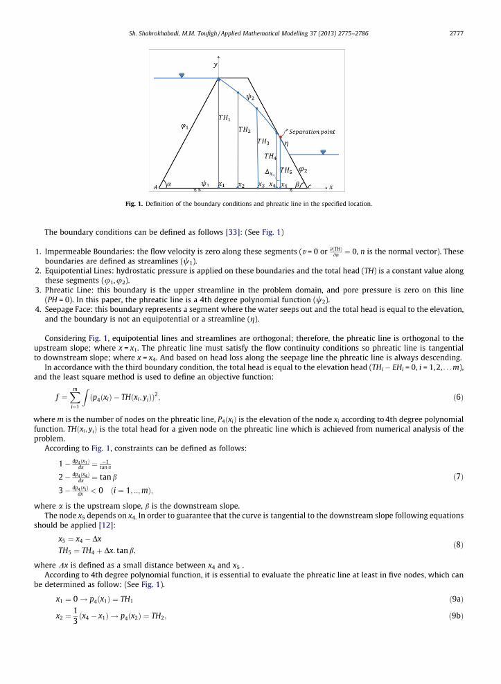
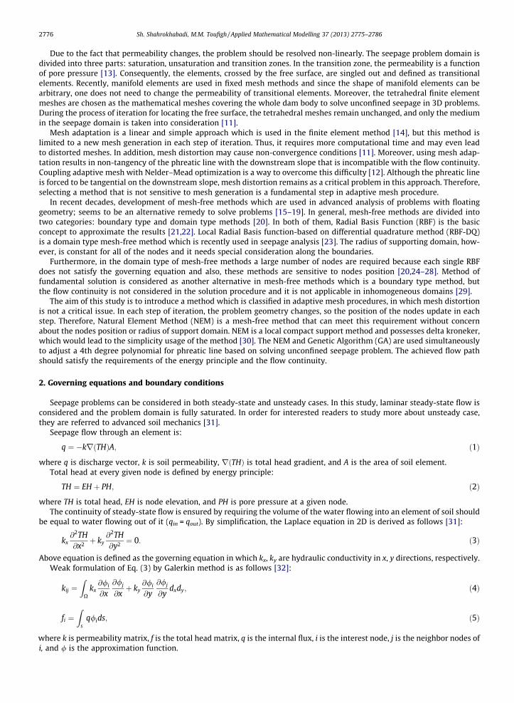
Fig. 1. Definition of the boundary conditions and phreatic line in the specified location.

Sh. Shahrokhabadi, M.M. Toufigh / Applied Mathematical Modelling 37 (2013) 2775–2786 2777

The boundary conditions can be defined as follows [33]: (See Fig. 1)

1. Impermeable Boundaries: the flow velocity is zero along these segments (v = 0 or @ðTHÞ@n ¼ 0, n is the normal vector). These

boundaries are defined as streamlines (w1).2. Equipotential Lines: hydrostatic pressure is applied on these boundaries and the total head (TH) is a constant value along

these segments (u1,u2).3. Phreatic Line: this boundary is the upper streamline in the problem domain, and pore pressure is zero on this line

(PH = 0). In this paper, the phreatic line is a 4th degree polynomial function (w2).4. Seepage Face: this boundary represents a segment where the water seeps out and the total head is equal to the elevation,

and the boundary is not an equipotential or a streamline (g).

Considering Fig. 1, equipotential lines and streamlines are orthogonal; therefore, the phreatic line is orthogonal to theupstream slope; where x = x1. The phreatic line must satisfy the flow continuity conditions so phreatic line is tangentialto downstream slope; where x = x4. And based on head loss along the seepage line the phreatic line is always descending.

In accordance with the third boundary condition, the total head is equal to the elevation head (THi � EHi = 0, i = 1,2, . . .m),and the least square method is used to define an objective function:

f ¼Xm

i¼1

Zðp4ðxiÞ � THðxi; yiÞÞ

2; ð6Þ

where m is the number of nodes on the phreatic line, P4ðxiÞ is the elevation of the node xi according to 4th degree polynomialfunction. THðxi; yiÞ is the total head for a given node on the phreatic line which is achieved from numerical analysis of theproblem.

According to Fig. 1, constraints can be defined as follows:

1� dp4ðx1Þdx ¼ �1

tan a

2� dp4ðx4Þdx ¼ tan b

3� dp4ðxiÞdx < 0 ði ¼ 1; ::;mÞ;

ð7Þ

where a is the upstream slope, b is the downstream slope.The node x5 depends on x4. In order to guarantee that the curve is tangential to the downstream slope following equations

should be applied [12]:

x5 ¼ x4 � DxTH5 ¼ TH4 þ Dx: tan b;

ð8Þ

where Dx is defined as a small distance between x4 and x5 .According to 4th degree polynomial function, it is essential to evaluate the phreatic line at least in five nodes, which can

be determined as follow: (See Fig. 1).

x1 ¼ 0! p4ðx1Þ ¼ TH1 ð9aÞ

x2 ¼13ðx4 � x1Þ ! p4ðx2Þ ¼ TH2; ð9bÞ

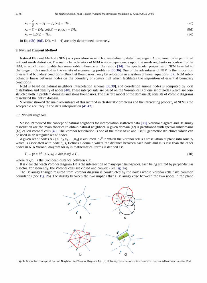
Fig. 2


x3 ¼23ðx4 � x1Þ ! p4ðx3Þ ¼ TH3; ð9cÞ

x4 ¼ C � TH4: cotðbÞ ! p4ðx4Þ ¼ TH4; ð9dÞx5 ! p4ðx5Þ ¼ TH5: ð9eÞ

In Eq. (9b)–(9d), THi(i = 2 � 4) are only determined iteratively.

3. Natural Element Method

Natural Element Method (NEM) is a procedure in which a mesh-free updated Lagrangian Approximation is permittedwithout mesh distortion. The main characteristics of NEM is its independency upon the mesh regularity in contrast to theFEM, in which mesh quality has remarkable influence on the results [34]. The spectacular properties of NEM have led tothe usage of this method in the variety of engineering problems [35,36]. One of the advantages of NEM is the impositionof essential boundary conditions (Dirichlet Boundaries), only by relocation in a system of linear equations [37]. NEM inter-polant is linear between nodes on the boundary of convex hull which facilitates the imposition of essential boundaryconditions.

NEM is based on natural neighbors interpolation scheme [38,39], and correlation among nodes is computed by localdistribution and density of nodes [40]. These interpolants are based on the Voronoi cells of one set of nodes which are con-structed both in problem domains and along boundaries. The discrete model of the domain (O) consists of Voronio diagramstessellated the entire domain.

Sukumar showed the main advantages of this method in elastostatic problems and the interesting property of NEM is theacceptable accuracy in the data interpolation [41,42].

3.1. Natural neighbors

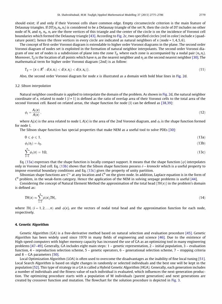
Sibson introduced the concept of natural neighbors for interpolation scattered data [38]. Voronoi diagram and Delaunaytessellation are the main theories to obtain natural neighbors. A given domain (X) is partitioned with special subdomains(Xi) called Voronoi cells [40]. The Voronoi tessellation is one of the most basic and useful geometric structures which canbe used in an irregular set of nodes.

A given set of nodes N = {n1,n2,n3, . . . ,nm} is assumed inR2 in which the Voronoi cell is a tessellation of plane into zone TI,

which is associated with node nI. TI Defines a domain where the distance between each node and nI is less than the othernodes in N. A Voronoi diagram for nI in mathematical terms is defined as:

TI ¼ fx 2 R2 : dðx; xIÞ < dðx; xJÞ8J – Ig; ð10Þ

where d(x,xi) is the Euclidean distance between x, xi.It is clear that each Voronoi diagram 1st is the intersection of many open half-spaces, each being limited by perpendicular

bisector. Consequently, the Voronoi cells are closed and convex. (See Fig. 2a).The Delaunay triangle resulted from Voronoi diagram is constructed by the nodes whose Voronoi cells have common

boundaries (See Fig. 2b). The duality between the two implies that a Delaunay edge between the two nodes in the plane

. Geometric concept of Natural Neighbor: (a) Voronoi Diagram 1st. (b) Delaunay Tessellation. (c) Circumcircle criteria. (d)Voronoi Diagram 2nd.


should exist; if and only if their Voronoi cells share common edge. Empty circumecircle criterion is the main feature ofDelaunay triangles. If DT(nJ,nk,nI) is considered to be a Delaunay triangle of the set N, then the circle of DT includes no othernode of N, and nj, nk, nI are the three vertices of this triangle and the center of the circle is on the incidence of Voronoi cellboundaries which formed the Delaunay triangle [43]. According to Fig. 2c, two specified circles (red in color) include x (quad-rature point); hence the three vertices in every circle are indicated as natural neighbors of x (node = 1,4,5,6).

The concept of first-order Voronoi diagram is extendable to higher order Voronoi diagrams in the plane. The second orderVoronoi diagram of nodes set is exploited in the formation of natural neighbor interpolants. The second order Voronoi dia-gram of one set of nodes is a subdivision of plane into the zone TIJ, where each zone is accompanied by a nodal pair (ni,nj).Moreover, TIJ is the location of all points which have ni as the nearest neighbor and nj as the second nearest neighbor [30]. Themathematical term for higher order Voronoi diagram (2nd) is as follow:

TIJ ¼ fx 2 R2 : dðx; xIÞ < dðx; xJÞ < dðx; xkÞg: ð11Þ

Also, the second order Voronoi diagram for node x is illustrated as a domain with bold blue lines in Fig. 2d.

3.2. Sibson interpolation

Natural neighbor coordinate is applied to interpolate the domain of the problem. As shown in Fig. 2d, the natural neighborcoordinate of x, related to node I (I = 1) is defined as the ratio of overlap area of their Voronoi cells to the total area of thesecond Voronoi cell. Based on related areas, the shape function for node (I) can be defined as [38,39]:

/I ¼AIðxÞAðxÞ ; ð12Þ

where AI(x) is the area related to node I, A(x) is the area of the 2nd Voronoi diagram, and /i is the shape function formedfor node I.

The Sibson shape function has special properties that make NEM as a useful tool to solve PDEs [30]:

0 6 / 6 1; ð13aÞ/IðxJÞ ¼ dIJ; ð13bÞXn

I¼1

/IðxÞ ¼ 1X; ð13cÞ

Eq. (13a) expresses that the shape function is locally compact support. It means that the shape function (u) interpolatesonly in Voronoi 2nd cell. Eq. (13b) shows that the Sibson shape functions possess d – kronockr which is a useful property toimpose essential boundary conditions and Eq. (13c) gives the property of unity partition.

Sibsonian shape functions are C1 at any location and C0 on the given node. In addition, Laplace equation is in the form ofC0 problem, in the weak-form category. Hence the application of the NEM in solving seepage problems is useful [44].

Considering the concept of Natural Element Method the approximation of the total head (THðxÞ) in the problem’s domainis defined as:

THðxÞ �Xn

i¼1

/ðxÞiTHi; ð14Þ

where THi ði ¼ 1;2; :::;nÞ and /(x)i are the vectors of nodal total head and the approximation function for each node,respectively.

4. Genetic Algorithm

Genetic Algorithm (GA) is a free-derivative method based on natural selection and evaluation procedure [45]. GeneticAlgorithm has been widely used since 1970 in many fields of engineering and science [46]. Due to the existence ofHigh-speed computers with higher memory capacity has increased the use of GA as an optimizing tool in many engineeringproblems [47–49]. Generally, GA includes eight main steps: 1 – genetic representation, 2 – initial population, 3 – evaluationfunction, 4 – reproduction selection scheme, 5 – genetic operators, 6 – generational selection scheme, 7 – stopping criteriaand 8 – GA parameters [50].

Local Optimization Algorithm (LOA) is often used to overcome the disadvantages as the inability of fine local tuning [51].Local Search Algorithm is based on slight changes in randomly or selected individuals and the best one will be kept in thepopulation [52]. This type of strategy in a GA is called a Hybrid Genetic Algorithm (HGA). Generally, each generation includesa number of individuals and the fitness value of each individual is evaluated, which influences the next-generation produc-tion. The optimizing procedure starts with a population of M individuals (parent generation) and next generations arecreated by crossover function and mutation. The flowchart for the solution procedure is depicted in Fig. 3.

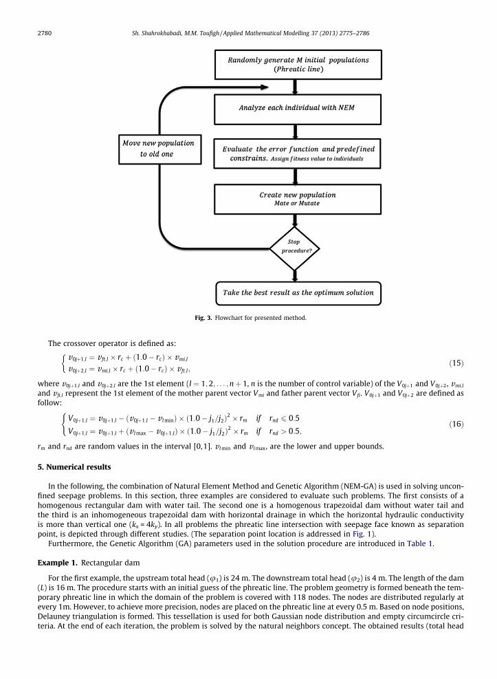
Fig. 3. Flowchart for presented method.


The crossover operator is defined as:

v0jþ1;l ¼ v ft;l � rc þ ð1:0� rcÞ � vmi;l

v0jþ2;l ¼ vmi;l � rc þ ð1:0� rcÞ � v ft;l;

�ð15Þ

where v0jþ1;l and v0jþ2;l are the 1st element (l ¼ 1;2; . . . ;nþ 1, n is the number of control variable) of the V0jþ1 and V0jþ2, vmi;l

and v fi;l represent the 1st element of the mother parent vector Vmi and father parent vector Vfi. V0jþ1 and V0jþ2 are defined asfollow:

V0jþ1;l ¼ v0jþ1;l � ðv0jþ1;l � v l minÞ � ð1:0� j1=j2Þ2 � rm if rnd 6 0:5

V0jþ1;l ¼ v0jþ1;l þ ðv l max � v0jþ1;lÞ � ð1:0� j1=j2Þ2 � rm if rnd > 0:5;

(ð16Þ

rm and rnd are random values in the interval [0,1]. v l min and v l max, are the lower and upper bounds.

5. Numerical results

In the following, the combination of Natural Element Method and Genetic Algorithm (NEM-GA) is used in solving uncon-fined seepage problems. In this section, three examples are considered to evaluate such problems. The first consists of ahomogenous rectangular dam with water tail. The second one is a homogenous trapezoidal dam without water tail andthe third is an inhomogeneous trapezoidal dam with horizontal drainage in which the horizontal hydraulic conductivityis more than vertical one (kx = 4ky). In all problems the phreatic line intersection with seepage face known as separationpoint, is depicted through different studies. (The separation point location is addressed in Fig. 1).

Furthermore, the Genetic Algorithm (GA) parameters used in the solution procedure are introduced in Table 1.

Example 1. Rectangular dam

For the first example, the upstream total head (u1) is 24 m. The downstream total head (u2) is 4 m. The length of the dam(L) is 16 m. The procedure starts with an initial guess of the phreatic line. The problem geometry is formed beneath the tem-porary phreatic line in which the domain of the problem is covered with 118 nodes. The nodes are distributed regularly atevery 1m. However, to achieve more precision, nodes are placed on the phreatic line at every 0.5 m. Based on node positions,Delauney triangulation is formed. This tessellation is used for both Gaussian node distribution and empty circumcircle cri-teria. At the end of each iteration, the problem is solved by the natural neighbors concept. The obtained results (total head

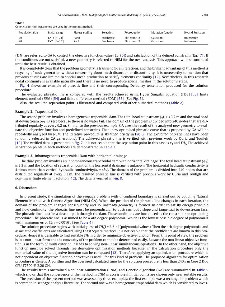
Table 1Genetic algorithm parameters are used in the present method.

Population size Initial range Fitness scaling Selection Reproduction Mutation function Hybrid Function

20 EX1: [4–24] Rank Stochastic Elit count: 2 Gaussian fminsearch20 EX2: [0–3.2] Rank Stochastic Elit count: 2 Gaussian fminsearch


ðTHÞ) are referred to GA to control the objective function value (Eq. (6)) and satisfaction of the defined constrains (Eq. (7)). Ifthe conditions are not satisfied, a new geometry is referred to NEM for the next analysis. This approach will be continueduntil the best result is obtained.

It is completely clear that the problem geometry is transient for all iterations, and the brilliant advantage of this method isrecycling of node generation without concerning about mesh distortion or discontinuity. It is noteworthy to mention thatprevious studies are limited to special mesh production to satisfy elements continuity [12]. Nevertheless, in this researchnodal continuity is available naturally and there is no need to produce special meshes in the solution’s steps.

Fig. 4 shows an example of phreatic line and their corresponding Delaunay tessellation produced for the solutionprocedure.

The evaluated phreatic line is compared with the results achieved using Hyper Singular Equation (HSE) [53], finiteelement method (FEM) [54] and finite difference method (FDM) [55]. (See Fig. 5).

Also, the resulted separation point is illustrated and compared with other numerical methods (Table 2).

Example 2. Trapezoidal Dam

The second problem involves a homogeneous trapezoidal dam. The total head at upstream (u1) is 3.2 m and the total headat downstream (u2) is zero because there is no water tail. The domain of the problem is divided into 240 nodes that are dis-tributed regularly at every 0.2 m. Similar to the previous example, GA uses the result of the analyzed new geometry to eval-uate the objective function and predefined constrains. Then, new optimized phreatic curve that is proposed by GA will berepeatedly analyzed by NEM. The iterative procedure is sketched briefly in Fig. 6. (The exhibited phreatic lines have beenrandomly selected in GA generations). The achieved phreatic line is verified with previous work by Ouria and Toufigh[12]. The verified data is presented in Fig. 7. It is noticeable that the separation point in this case is x4 and TH4. The achievedseparation points in both methods are demonstrated in Table 3.

Example 3. Inhomogeneous trapezoidal Dam with horizontal drainage

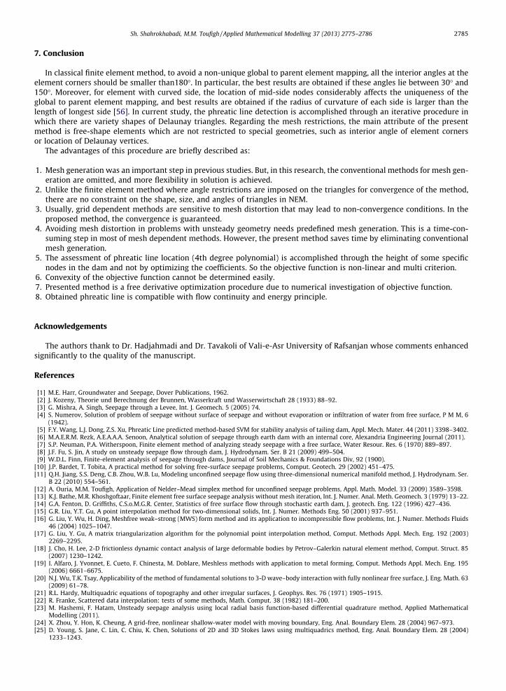
The third problem involves an inhomogeneous trapezoidal dam with horizontal drainage. The total head at upstream (/1)is 3.2 m and the location of separation point on the horizontal drainage is unknown. The horizontal hydraulic conductivity is4 times more than vertical hydraulic conductivity(kx = 4ky). The domain of the problem is divided into 240 nodes that aredistributed regularly at every 0.2 m. The resulted phreatic line is verified with previous work by Ouria and Toufigh andnon-linear finite element solution [12]. The data is verified in Fig. 8.

6. Discussion

In present study, the simulation of the seepage problem with unconfined boundary is carried out by coupling NaturalElement Method with Genetic Algorithm (NEM-GA). When the position of the phreatic line changes in each iteration, thedomain of the problem changes consequently and so, unsteady geometry is formed. In order to satisfy energy principleand flow continuity, the phreatic line must be perpendicular to upstream body slope and tangential to downstream face.The phreatic line must be a descent path through the dam. These conditions are introduced as the constraints in optimizingprocedure. The phreatic line is assumed to be a 4th degree polynomial which is the lowest possible degree of polynomialswith minimum error (Err = 0.0016). (See Table 4).

The solution procedure begins with initial guess of THi(i = 2,3,4) (polynomial values). Then the 4th degree polynomial andassociated coefficients are calculated using Least Square method. It is noticeable that the coefficients are known in this pro-cedure. Hence it is desirable to find suitable THi in order to minimize objective function. From this point of view the problemis in a non-linear form and the convexity of the problem cannot be determined easily. Because the non-linear objective func-tion is in the form of multi criterion it leads to solving non-linear simultaneous equations. On the other hand, the objectivefunction must be solved through free derivative optimization methods because; in the calculation procedure only thenumerical value of the objective function can be computed [12]. Therefore, applying an optimization procedure which isnot dependent on objective function derivative is useful for this kind of problem. The proposed algorithm for optimizationprocedure is Genetic Algorithm and the averaged calculated time for the solution procedure is less than 240 s in Core 2 DuoCPU T7500 @ 2.20 GHz.

The results from Constrained Nonlinear Minimization (CNM) and Genetic Algorithm (GA) are summarized in Table 5which shows that the convergence of the method in CNM is accessible if initial points are chosen only near suitable results.

The precision of the present method was assessed by three examples: the first example was a rectangular problem whichis common in seepage analysis literature. The second one was a homogenous trapezoidal dam which is considered to inves-

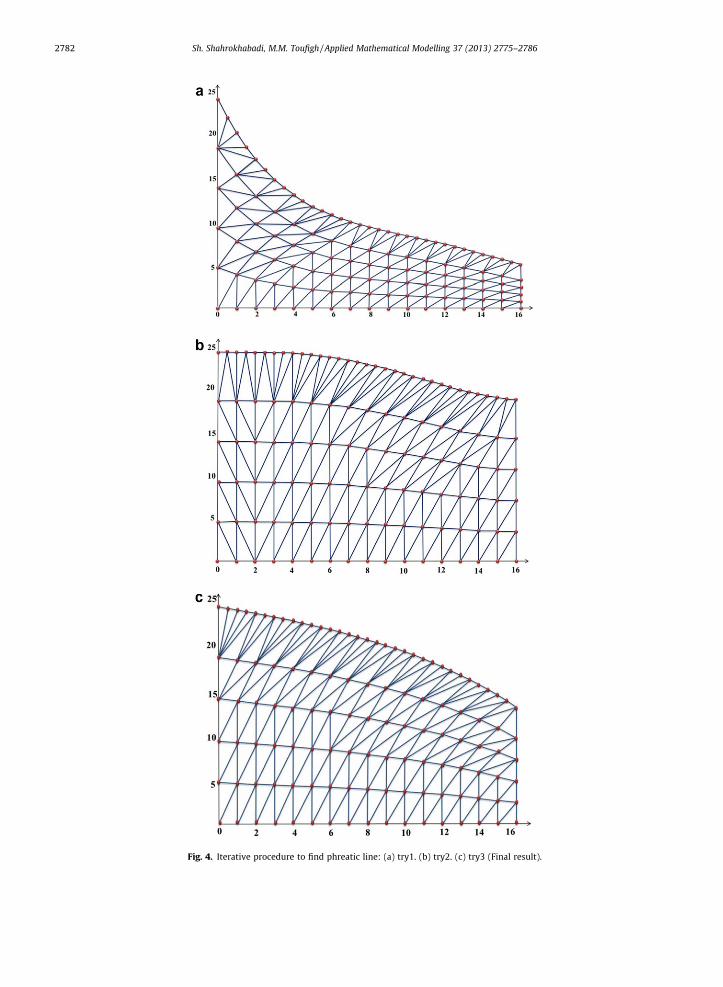
Fig. 4. Iterative procedure to find phreatic line: (a) try1. (b) try2. (c) try3 (Final result).


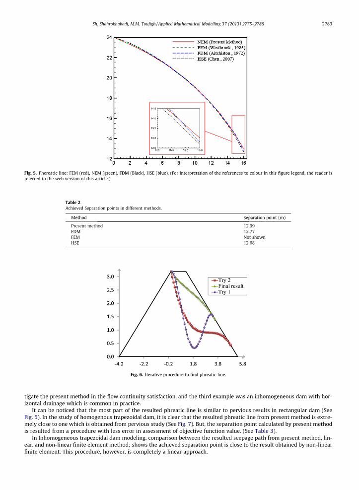
Fig. 5. Phereatic line: FEM (red), NEM (green), FDM (Black), HSE (blue). (For interpretation of the references to colour in this figure legend, the reader isreferred to the web version of this article.)

Table 2Achieved Separation points in different methods.

Method Separation point (m)

Present method 12.99FDM 12.77FEM Not shownHSE 12.68

Fig. 6. Iterative procedure to find phreatic line.


tigate the present method in the flow continuity satisfaction, and the third example was an inhomogeneous dam with hor-izontal drainage which is common in practice.

It can be noticed that the most part of the resulted phreatic line is similar to pervious results in rectangular dam (SeeFig. 5). In the study of homogenous trapezoidal dam, it is clear that the resulted phreatic line from present method is extre-mely close to one which is obtained from pervious study (See Fig. 7). But, the separation point calculated by present methodis resulted from a procedure with less error in assessment of objective function value. (See Table 3).

In Inhomogeneous trapezoidal dam modeling, comparison between the resulted seepage path from present method, lin-ear, and non-linear finite element method; shows the achieved separation point is close to the result obtained by non-linearfinite element. This procedure, however, is completely a linear approach.

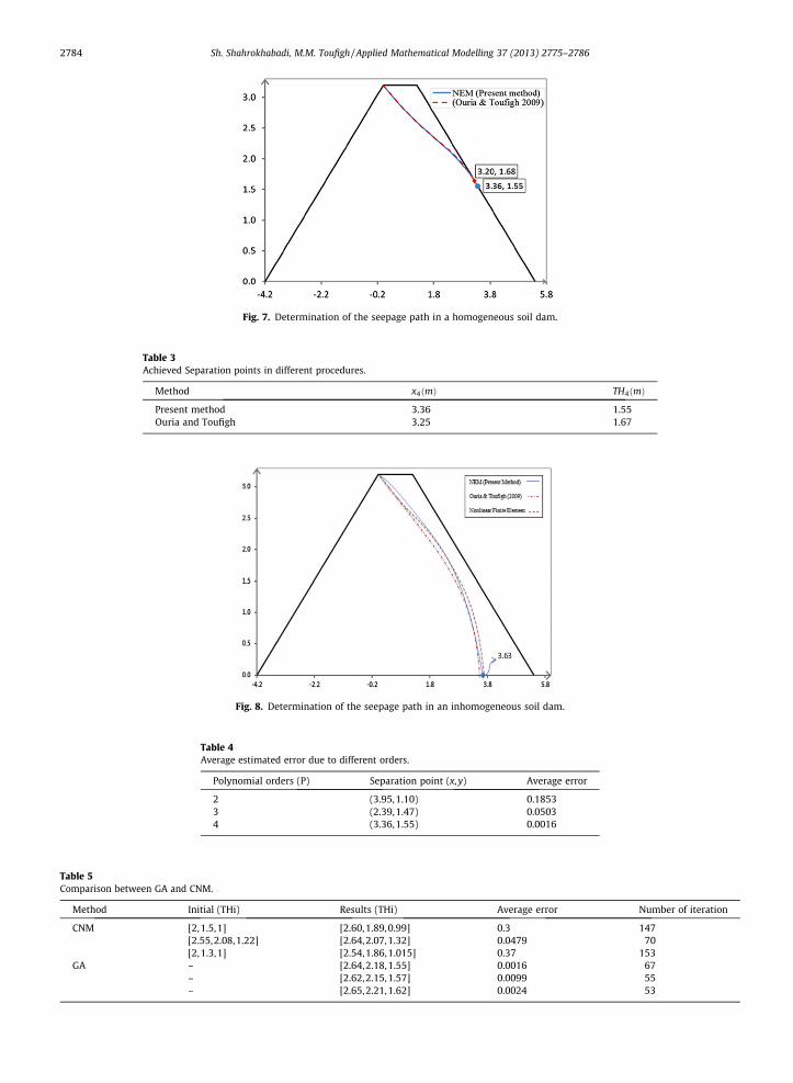
Fig. 7. Determination of the seepage path in a homogeneous soil dam.

Table 3Achieved Separation points in different procedures.

Method x4ðmÞ TH4ðmÞ

Present method 3.36 1.55Ouria and Toufigh 3.25 1.67

Fig. 8. Determination of the seepage path in an inhomogeneous soil dam.

Table 4Average estimated error due to different orders.

Polynomial orders (P) Separation point (x,y) Average error

2 (3.95,1.10) 0.18533 (2.39,1.47) 0.05034 (3.36,1.55) 0.0016

Table 5Comparison between GA and CNM.

Method Initial (THi) Results (THi) Average error Number of iteration

CNM [2,1.5,1] [2.60,1.89,0.99] 0.3 147[2.55,2.08,1.22] [2.64,2.07,1.32] 0.0479 70[2,1.3,1] [2.54,1.86,1.015] 0.37 153

GA – [2.64,2.18,1.55] 0.0016 67– [2.62,2.15,1.57] 0.0099 55– [2.65,2.21,1.62] 0.0024 53



7. Conclusion

In classical finite element method, to avoid a non-unique global to parent element mapping, all the interior angles at theelement corners should be smaller than180�. In particular, the best results are obtained if these angles lie between 30� and150�. Moreover, for element with curved side, the location of mid-side nodes considerably affects the uniqueness of theglobal to parent element mapping, and best results are obtained if the radius of curvature of each side is larger than thelength of longest side [56]. In current study, the phreatic line detection is accomplished through an iterative procedure inwhich there are variety shapes of Delaunay triangles. Regarding the mesh restrictions, the main attribute of the presentmethod is free-shape elements which are not restricted to special geometries, such as interior angle of element cornersor location of Delaunay vertices.

The advantages of this procedure are briefly described as:

1. Mesh generation was an important step in previous studies. But, in this research, the conventional methods for mesh gen-eration are omitted, and more flexibility in solution is achieved.

2. Unlike the finite element method where angle restrictions are imposed on the triangles for convergence of the method,there are no constraint on the shape, size, and angles of triangles in NEM.

3. Usually, grid dependent methods are sensitive to mesh distortion that may lead to non-convergence conditions. In theproposed method, the convergence is guaranteed.

4. Avoiding mesh distortion in problems with unsteady geometry needs predefined mesh generation. This is a time-con-suming step in most of mesh dependent methods. However, the present method saves time by eliminating conventionalmesh generation.

5. The assessment of phreatic line location (4th degree polynomial) is accomplished through the height of some specificnodes in the dam and not by optimizing the coefficients. So the objective function is non-linear and multi criterion.

6. Convexity of the objective function cannot be determined easily.7. Presented method is a free derivative optimization procedure due to numerical investigation of objective function.8. Obtained phreatic line is compatible with flow continuity and energy principle.

Acknowledgements

The authors thank to Dr. Hadjahmadi and Dr. Tavakoli of Vali-e-Asr University of Rafsanjan whose comments enhancedsignificantly to the quality of the manuscript.

References

[1] M.E. Harr, Groundwater and Seepage, Dover Publications, 1962.[2] J. Kozeny, Theorie und Berechnung der Brunnen, Wasserkraft und Wasserwirtschaft 28 (1933) 88–92.[3] G. Mishra, A. Singh, Seepage through a Levee, Int. J. Geomech. 5 (2005) 74.[4] S. Numerov, Solution of problem of seepage without surface of seepage and without evaporation or infiltration of water from free surface, P M M, 6

(1942).[5] F.Y. Wang, L.J. Dong, Z.S. Xu, Phreatic Line predicted method-based SVM for stability analysis of tailing dam, Appl. Mech. Mater. 44 (2011) 3398–3402.[6] M.A.E.R.M. Rezk, A.E.A.A.A. Senoon, Analytical solution of seepage through earth dam with an internal core, Alexandria Engineering Journal (2011).[7] S.P. Neuman, P.A. Witherspoon, Finite element method of analyzing steady seepage with a free surface, Water Resour. Res. 6 (1970) 889–897.[8] J.F. Fu, S. Jin, A study on unsteady seepage flow through dam, J. Hydrodynam. Ser. B 21 (2009) 499–504.[9] W.D.L. Finn, Finite-element analysis of seepage through dams, Journal of Soil Mechanics & Foundations Div, 92 (1900).

[10] J.P. Bardet, T. Tobita, A practical method for solving free-surface seepage problems, Comput. Geotech. 29 (2002) 451–475.[11] Q.H. Jiang, S.S. Deng, C.B. Zhou, W.B. Lu, Modeling unconfined seepage flow using three-dimensional numerical manifold method, J. Hydrodynam. Ser.

B 22 (2010) 554–561.[12] A. Ouria, M.M. Toufigh, Application of Nelder–Mead simplex method for unconfined seepage problems, Appl. Math. Model. 33 (2009) 3589–3598.[13] K.J. Bathe, M.R. Khoshgoftaar, Finite element free surface seepage analysis without mesh iteration, Int. J. Numer. Anal. Meth. Geomech. 3 (1979) 13–22.[14] G.A. Fenton, D. Griffiths, C.S.o.M.G.R. Center, Statistics of free surface flow through stochastic earth dam, J. geotech. Eng. 122 (1996) 427–436.[15] G.R. Liu, Y.T. Gu, A point interpolation method for two-dimensional solids, Int. J. Numer. Methods Eng. 50 (2001) 937–951.[16] G. Liu, Y. Wu, H. Ding, Meshfree weak–strong (MWS) form method and its application to incompressible flow problems, Int. J. Numer. Methods Fluids

46 (2004) 1025–1047.[17] G. Liu, Y. Gu, A matrix triangularization algorithm for the polynomial point interpolation method, Comput. Methods Appl. Mech. Eng. 192 (2003)

2269–2295.[18] J. Cho, H. Lee, 2-D frictionless dynamic contact analysis of large deformable bodies by Petrov–Galerkin natural element method, Comput. Struct. 85

(2007) 1230–1242.[19] I. Alfaro, J. Yvonnet, E. Cueto, F. Chinesta, M. Doblare, Meshless methods with application to metal forming, Comput. Methods Appl. Mech. Eng. 195

(2006) 6661–6675.[20] N.J. Wu, T.K. Tsay, Applicability of the method of fundamental solutions to 3-D wave–body interaction with fully nonlinear free surface, J. Eng. Math. 63

(2009) 61–78.[21] R.L. Hardy, Multiquadric equations of topography and other irregular surfaces, J. Geophys. Res. 76 (1971) 1905–1915.[22] R. Franke, Scattered data interpolation: tests of some methods, Math. Comput. 38 (1982) 181–200.[23] M. Hashemi, F. Hatam, Unsteady seepage analysis using local radial basis function-based differential quadrature method, Applied Mathematical

Modelling (2011).[24] X. Zhou, Y. Hon, K. Cheung, A grid-free, nonlinear shallow-water model with moving boundary, Eng. Anal. Boundary Elem. 28 (2004) 967–973.[25] D. Young, S. Jane, C. Lin, C. Chiu, K. Chen, Solutions of 2D and 3D Stokes laws using multiquadrics method, Eng. Anal. Boundary Elem. 28 (2004)

1233–1243.


[26] Q. Ma, Meshless local Petrov–Galerkin method for two-dimensional nonlinear water wave problems, J. Comput. Phys. 205 (2005) 611–625.[27] C. Du, An element-free Galerkin method for simulation of stationary two-dimensional shallow water flows in rivers, Comput. Methods Appl. Mech.

Eng. 182 (2000) 89–107.[28] R. Ata, A. Soulaïmani, A stabilized SPH method for inviscid shallow water flows, Int. J. Numer. Methods Fluids 47 (2005) 139–159.[29] K. Chaiyo, P. Rattanadecho, S. Chantasiriwan, The method of fundamental solutions for solving free boundary saturated seepage problem, Int. Commun.

Heat Mass Transfer 38 (2011) 249–254.[30] N. Sukumar, The Natural Element Method in Solid Mechanics, Northwestern University, 1998.[31] B.M. Das, Advanced Soil Mechanics, Routledge, 2008.[32] J.T. Christian, C.S. Desai, Numerical Methods in Geotechnical Engineering, McGraw-Hill, 1977.[33] J.J. Connor, C.A. Brebbia, Finite Element Techniques for Fluid Flow, Newnes Butterworths, London, 1976. 317 p., 1.[34] D. González, E. Cueto, F. Chinesta, M. Doblaré, A natural element updated Lagrangian strategy for free-surface fluid dynamics, J. Comput. Phys. 223

(2007) 127–150.[35] J. Cho, H. Lee, 2-D large deformation analysis of nearly incompressible body by natural element method, Comput. Struct. 84 (2006) 293–304.[36] C. Yongchang, Z. Hehua, A meshless local natural neighbour interpolation method for stress analysis of solids, Eng. Anal. Boundary Elem. 28 (2004)

607–613.[37] E. Cueto, J. Cegonino, B. Calvo, M. Doblaré, On the imposition of essential boundary conditions in natural neighbour Galerkin methods, Commun.

Numer. Methods Eng. 19 (2003) 361–376.[38] R. Sibson, A Vector Identity for the Dirichlet Tessellation, Cambridge Univ Press, 1980.[39] R. Sibson, A brief description of natural neighbour interpolation, Interpreting multivariate data, 21 (1981).[40] N. Sukumar, B. Moran, A. Yu Semenov, V. Belikov, Natural neighbour Galerkin methods, Int. J. Numer. Methods Eng. 50 (2001) 1–27.[41] D. Gonzalez, E. Cueto, M. Martinez, M. Doblaré, Numerical integration in natural neighbour Galerkin methods, Int. J. Numer. Methods Eng. 60 (2004)

2077–2104.[42] N. Sukumar, B. Moran, C 1 natural neighbor interpolant for partial differential equations, Numer. Methods Partial Differ. Equat. 15 (1999) 417–447.[43] C.L. Lawson, Software for C1 interpolation (1977).[44] S. Shahrokhabadi, M. Toufigh, R. Gholizadeh, Application of Natural Element Method in Solving Seepage Problem, in ASCE, 2010.[45] A. Javadi, R. Farmani, T. Tan, A hybrid intelligent genetic algorithm, Adv. Eng. Inform. 19 (2005) 255–262.[46] J.D. Bagley, The behavior of adaptive systems which employ genetic and correlation algorithms (1967).[47] D.E. Goldberg, The Design of Innovation: Lessons from and for Competent Genetic Algorithms, Springer, 2002.[48] L.M. Schmitt, Theory of genetic algorithms, Theoret. Comput. Sci. 259 (2001) 1–61.[49] S. Sivanandam, S. Deepa, Introduction to Genetic Algorithms, Springer-Verlag, Berlin, Heidelberg, 2008.[50] R. Farmani, J.A. Wright, Self-adaptive fitness formulation for constrained optimization, IEEE Trans. Evolutionary Comput. 7 (2003) 445–455.[51] K.W. Kim, S.W. Baek, Inverse surface radiation analysis in an axisymmetric cylindrical enclosure using a hybrid genetic algorithm, Numer. Heat

Transfer, Part A: Applications 46 (2004) 367–381.[52] L. Gosselin, M. Tye-Gingras, F. Mathieu-Potvin, Review of utilization of genetic algorithms in heat transfer problems, Int. J. Heat Mass Transfer 52

(2009) 2169–2188.[53] J.T. Chen, C.C. Hsiao, Y.P. Chiu, Y.T. Lee, Study of free surface seepage problems using hypersingular equations, Commun. Numer. Methods Eng. 23

(2007) 755–769.[54] J. Aitchison, Numerical treatment of a singularity in a free boundary problem, Proc. Roy. Soc. Lond. A. Math. Phys. Sci. 330 (1972) 573–580.[55] D. Westbrook, Analysis of inequality and residual flow procedures and an iterative scheme for free surface seepage, Int. J. Numer. Methods Eng. 21

(1985) 1791–1802.[56] D.M. Potts, L. Zdravkovi, Finite Element Analysis in Geotechnical Engineering: Theory, Thomas Telford Services Ltd, 2001.

Documents

The Solution of Unconfined Seepage Problem Using Natural Element Method (NEM) Coupled With Genetic Algorithm (GA)