New Zealand Geomechanics Society Groundwater and Seepage Symposium 24-25 May 1990, Auckland University

Calculating seepage flow with a free surf ace: Some old methods and some new ones

John D. Fenton

Department of Civil Engineering University of Auckland Private Bag, Auckland

ABSTRACT

The main aim of this paper is to describe and review a family of approximate methods for groundwater flqw with a free surface. It is the intention to show that the appfoximate methods, with some innovations, are capable of describing a range of problems, and it is not always necessary to go to the complications of finite element and boundary element methods.

The nature of unconfined seepage flow is examined, and the nonlinear free surface condition is obtained. An additional equation is derived which is shown to be exact, and which is rather more convenient for developing methods of solution. Then some traditional approximate methods for free surface problems are described. A method of higher-order approxima­tion is introduced, then some simple approximations for flow in the upstream region of a darn are obtained. Subsequently methods for flow over curved topography are examined, and the paper ends with the development of a numerical method for solving the family of equations obtained.

INTRODUCTION

Consider an incompressible fluid flowing in a non-deformable soil mass, which is assumed to be isotropic and homogeneous with conductivity K. The purpose of this paper is to consider the complications introduced by the existence of a free surface, and so complications associated with variation of material pro­perties have not been introduced. Darcy's law for the specific discharge u (the macroscopic fluid velocity) is u= -KV¢, where ¢ is the piezometric head. The statement of mass conservation is V • u = 0, which as the medium is assumed to be homogeneous (K constant) gives Laplace's equation valid throughout the flow:

v2¢ = a2¢ + a2¢ + a2¢ = o. (1) ax 2 ay 2 az 2

In problems where the flow has no free surface, a typical prob­lem is to solve equation (1) in a closed region subject to rela­tively simple conditions on the boundary, for example (i) that ¢ be a constant over a submerged boundary at any or all instants in time, (ii) that on an impervious boundary the normal velocity is zero, leading to the condition a¢/an = 0, where n is a local co-ordinate normal to the boundary, and (iii) that on a seepage face ¢ is equal to the elevation.

Seepage flow with a free surface

If a flow has a water table (phreatic surface) as its upper boun­dary, solution becomes more difficult because of the nonlinearity of the boundary condition (to be established below) and because the location of the boundary is also an unknown of the problem. Such a flow is often called "unconfined".

z y

Figure 1. Unconfined flow over an impermeable bed.

Consider the unconfined flow shown in Figure 1. The z axis is chosen to be vertical upwards. Fluid is accreting by flowing downwards through the unsaturated soil above the main flow, with a velocity (volume flux per unit area) of N. We write this as a vector N = - kN, where k is a unit vector in the z direction. The actual velocity of fluid particles on the free surface is V, related to the other velocities by

(u- N).n= neV .n, (2)

(Bear, 1972, #7.1.6), in which ne is the effective porosity and n is a unit vector perpendicular to the surface. TI1is equation expresses conservation of fluid volume across the surface.

The condition that the pressure p at a moving particle remain atmospheric is

§p__+VVp=O at · '

(3)

but on the free surface ~ = z, thus Bp/Bt = pg 8¢/at, where p is fluid density and g is gravitational acceleration, and, Vp = pg(V¢-Vz) = pg(V¢-k). As the free surface has constant p, then Vp is perpendicular to it and is in the direction of n. Hence it can replace n in equation (2), giving after some mani­pulation,

neE/t-K [¢J+¢]+¢}]+¢y(N+K)-N= 0, (4)

where the subscripts denote partial differentiation. This is valid on the free surface z = h (x, y, t ). As the equation contains squares of terms in ¢ it is nonlinear, which makes analytical solution very difficult and it is not possible to combine solutions linearly as is possible in confined flow.

In the special case of two-dimensional steady flow, the boundary is more easily expressed in terms of the streamfunclion -,P. If mass-conservation is satisfied in two dimensions, then a stream­function -,P exists such that the x and y velocity components, u and v respectively are given by

u = - K §1_ and v = + K §1_. ay ax

If the velocity field obeys Darcy's law, then it is irrotational such that V x u = 0, and substituting the expressions for velocity shows that

vz-,µ= az-,µ + a2-,p = o. ax 2 ay 2

It can be shown that on any streamline in steady flow, -,P is con­stant if there is no accretion. It has the important significance that the difference in -,P between two streamlines gives the volume flux per unit width between those streamlines. Thus, if -,P = 0 on the underlying impermeable layer, then -,P = - Q/K on the free surface, where Q is the volume f!µx per unit width nor­mal to the flow.

Integrated form of the mass-conservation equation

If the mass-conservation equation is integrated vertically over the depth of the flow, from the impermeable layer to the free surface, an equation is obtained which can be used to derive a family of solution methods, and is easier to deal with than the boundary condition (4). In this work we show that the equation obtained is actually exact, an unusual result which seems not to be widely known.

N

Oy

u+ou

Figure 2. Control volume used in derivation.

We consider the control volume which is the elemental prism of plan dimension ox and oy shown in Figure 2. It is important and considerably simpler to allow the control volume to extend beyond the level of the free surface, which as it is in the inte­rior, does not have to be treated specially. The volume fluxes entering the face perpendicular to the x direction and leaving via the opposite face are, respectively

liy f u dz and oy f [u + /ix .El!:_] dz , Zb Zb ax

where the vertical integration is from a point on the bed z = z b (x, y ) to one on the free surface z = h (x, y, t ) .

By subtracting one of these from the other to obtain the net volume flux, performing a similar operation for the other faces for the v velocity, considering an elemental time increment tit in

which the surface has risen to give an incremental volume stored neah/at Ot /ix liy and an accreted volume Not ox liy, then by taking the limit as each of the elemental lit, 5x and liy go to zero, the integrated mass-conservation equation is obtained:

a1 a [1i l a [1i l ne -f + -a f u dz + - f v dz = N . f X Zb ay Zb

(5)

This equation is exact, and as such is a relative rarity in free­surface flows, or in fluid mechanics in general. The author has not been able to find it in the seepage flow literature, although an equivalent exists for free-surface flow in coastal and hydraulic engineering. The traditional derivation assumes that tile velocity components are constant over a vertical line. We now proceed to make this approximation, after which a more accurate one will be studied.

DUPUIT'S APPROXIMATION AND FORCHHEIMER'S EQUATION

If both u and v in equation (5) are assumed to be independent of z such that the head gradient also is independent of z and is given by the gradient of the surface elevation, then the integrals can be approximated by

f u dz :::: u f dz= -K~ [1i - zb). Zb Zb ax

The otherwise authoritative Bear ( 1972, p362) is incorrect in stating that the vertical flow components have been ignored.

Making the same approximation for flow in they direction, sub­stituting into equation (5) gives

ah a ( ah ( ) J a ( ah ( ) ] ne- = - K- h - zb + - K- h - zb + N. (6) at ax ax ay ay

This is a partial differential equation governing the surface elevation h as a function of time t and horizontal co-ordinates x and y. It is necessary to know the initial conditions in time and the boundary values in the space co- ordinates. It is a non-1 inear equation, and one which incorporates the effects of topo­graphic variation via the bed elevation zb. In the case of unsteady problems, it is necessary to be able to evaluate the spa­tial derivatives on the right side so that the rate of change in time calculated and the solution updated, in an essentially linear process. For steady problems, however, the left side is zero and the nonlinear problem has to be solved.

For a homogeneous aquifer (K constant) and where the bed is horizontal (zb = 0), the equation simplifies to Forchheimer's equation:

!!_<:_ ~ = .l__ [h .£.!2. ] + _E_ [h .E.f2. ] + N K at ax ax ay ay K

a2 ( 1 J a2

( 1 J N = -- -h2 + -- -h2 + -. - ax 2 2 ay 2 2 K

(7)

A number of analytical solutions to this equation are given in Bear ( 1972, #8.2). The well-known two-dimensional example of steady flow between two vertical-sided reservoirs is obtained by eliminating the t and y variation, so that equation (7) becomes

d 2 ( 1 2) N -- -h + -= 0 dx2 2 K ,

which can be solved to give the solution

h 2 - ht N h 2 = h 2 - 0 x + -(L - x )x

0 L K '

. where h0 is the surface elevation at x = 0 and hL at x = L. A useful result from that solution is the volume flux through the faces, and is obtained using the result that u = - Kdh/dx:

Qo K ( 2 2] - NL QL = 2L ho - lzL + z·

Despite the approximations made, it is a remarkable fact that this expression for the volume flux is exact for the vertical-sided case!

The most powerful feature of Forchheimer's general equation (7) for steady flow is that it is an equation linear in the variable h 2/2, and all of the techniques of harmonic analysis are avail­able for solution. The flavour of the solutions can be obtained by considering a dewatering problem in which four wells at the corners of a site, are located at (a, a), (a, -a), (-a, a) and (-a, -a), and each well discharges a volume rate Q. The solu­tion is

th 2 = -/;x (1og ((x - a) 2 + (y - a) 2)

+ 3 other combinations of (x ±a ) 2 and (y ±a )2 J .

A HIGHER APPROXIMATION

In this section we obtain a more-accurate equation governing motion with a free surface, and show that Forchheimer's equa­tion is obtained as the lowest level of approximation. Consider the motion of a layer of unconfined fluid over a horizontal bed. Instead of assuming that the head is constant over a vertical line we allow it to vary quadratically between the surface and the bottom. Let the head at any point be given by the expansion

</>=h-i[z 2 -1i 2 ]vz21i, (8)

in which ¢ (x, y, z, t) is the piezometric head at any point, h (x, y, t) is the thickness of the fluid layer above that point, and V} is the two-dimensional Laplacian operator V} = a2jax 2 + a2jay 2. This expansion is typical of that obtained from shallow-water theories in coastal hydrodynamics and hydraulic engineering. It is assumed that variation in the horizontal (with x and y) has a much longer length scale than in the vertical. This means that the assumed form satisfies Laplace's equation in three dimensions, as v} acting on the second term can be shown to be relatively small.

In addition to satisfying the field equation, substitution shows that ¢ = h on the water table surface as it should, and differentiation shows that a¢/az = 0 on the bottom, when z = 0. It remains to satisfy the nonlinear surface condition, equation ( 4), which was done by Dagan ( 1967) using a complicated pro­cedure expanding in powers of a small parameter. It is, in fact rather easier to incorporate this condition by substituting into the integrated mass-conservation equation (5). Using Darcy's law and a little manipulation gives the result:

(9)

After some manipulation, and inferring that some of Dagan's results contain typographical errors it can be shown that his complicated expressions reduce to this rather simpler expression. If the last term is neglected, then Forchheimer's equation (7) is recovered. It is perhaps surprising that the addition of variation in the vertical has not complicated the equation more than by the addition of a single term.

In the important special case of steady one-dimensional flow without accretion, the equation becomes, after integrating twice with respect to x , simple to do in this case:

1-113 d2h + 1 I 2 A B - -z = x+ 3 dx2 2 '

(10)

where A and B are constants. It can be shown that A is actu­ally - Q/K, where Q is the unit volume flux. Equation ( 10) is a ·

second-order differential equation representing the surface profile of a steady seepage flow, allowing for variation in the vertical. The equation is nonlinear and is apparently difficult to solve analytically. However, numerical solution by standard methods such as Runge-Kutta should not be difficult.

FREE SURFACE FLOW THROUGH A DAM

In this section a convenient approximation is obtained for flow in the upstream and central parts of a dam.

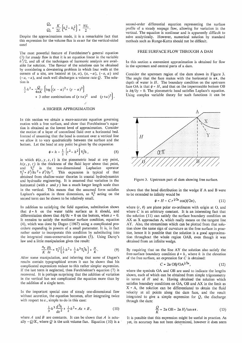
Consider the upstream region of the dam shown in Figure 3. The angle that the face makes with the horizontal is a7r, the depth of water is H. The boundary condition on the upstream face OA is that ¢ = H, and that on the impermeable bottom OB is a¢/ay = O. The piezometric head satisfies Laplace's equation. Using complex variable theory for such functions it can be

. I . T .~.·.·

.. > ·>: >> < > T> .y. ..

H . . >Y >

. <<>.T> <>y<>····· . +·.·.·.···

.. .... . r· .. .............. ·:.·:.1·:. : .

..... ... T ...

.·.·. <<><>>>+>··· ..... , ..

Figure 3. Upstream part of dam showing free surface.

shown that the head distribution in the wedge if A and B were to be extended to infinity would be

¢ = H - C rV2a cos(0/2o:), (11)

where (r, 0) arc plane polar co-ordinates with origin at 0, and where C is an arbitrary constant. It is an interesting fact that the solution (11) can satisfy the surface boundary condition on AX as X approaches A, which really means on the tangent line A Y. Also, the streamlines which can be plotted from that solu­tion show the same sign of curvature as the free surface in prac­tice, hence it is possible that the solution is a good approxima­tion throughout the whole region OAB, even though it was obtained from an infinite wedge.

By requiring that on the line A Y the solution also satisfy the free-surface boundary condition ¢ = h, where lz is the elevation of the free surface, an expression for C is obtained:

C = 2o: OB/OA1/2a, ( 12)

where the symbols OA and OB are used to indicate the lengths shown, each of which can be obtained from simple trigonometry in terms of H and a. Having obtained the solution which satisfies boundary conditions on OA, OB and AX in the limit as X _, A, the solution can be differentiated to obtain the fluid velocity al all points along the dam face, and the result integrated to give a simple expression for Q, the discharge through the dam:

f = 2a OB= 2a H/tanmr. (13)

·1t is possible that this expression might be useful in practice. As yet, its accuracy has not been det~;mined, however it does seem

to have one defect, that in the limit as the dam wall becomes vertical it gives zero discharge. This limit might not be thought to be practical, but it has been used a lot in conjunction with Dupuit's approximation.

Although the above theory is as yet untested, it is interesting to compute the distribution of piezometric head on the vertical line AB, to compare with Dupuit's assumptions. The region to the right of AB is simply that of free surface flow over a horizontal bed, which should be well approximated by the Dupuit theory or more accurately by the theory given in the previous section, where quadratic variation in the vertical was allowed.

The quadratic distribution

¢(x AB• Y) = ¢B + (¢A- ¢B) []Ir (14)

interpolates between the value of ¢ at A and that at 13 and satisfies the boundary condition on the bed. By requiring the approximate solution of equation (11) 'iind (12) to give the values o( ¢A and ¢ B• the solution is obtained:

¢(xAn1Y)=H-COI31/2a(1-7ff. (15)

The comparison between this simple quadratic approximation and the solution ( 11) is given in Figure 4 for a batter gradient of 2:1 (a slope of 1/2). It can be seen that the agreement is excellent, and the two are indistinguishable at this scale. For steeper batters (up to 1:1 was tested) the two agreed to four significant figures!

The possible importance of this lies in the fact that the head variation in the vertical is not constant, but shows marked qua­dratic variation, hence the Dupuit approximation may have to be re-examined for such problems. What is remarkable, how­ever, is that quadratic variation seems to describe the head so accurately. With this variation it would seem possible that the theory of the previous section which allows for quadratic varia­tion might be helpful in obtaining approximate solutions to flow through dams.

1.0

z/11

0.5

0

--- Eqnaliou (11)

Qua<lrnlic approx. (15)

0.5 1.0

Figure 4. Head distribution on AB. Comparison between Equations (11) and (15).

SHALLOW FLOW OVER A CURVED IMPERMEABLE BOUNDARY

Consider the unsteady two-dimensional flow with a free surface shown in Figure 5: An orthogonal curvilinear co-ordinate sys­tem (s, 11) is introduced, in which s is the arc length along the bed and n is perpendicular to it. The free surface is 11 = lz (s, t ), where t is time; the bed is 11 = 0. At any points, 0 is the angle of declination of the bed, and the local curvature of

Free surface

s

Figure 5. Physical problem and (s, n) co-ordinate system.

the bed "' is given by 1<;(s) = -d B(s )/ds, where the curvature is l/R, in which R is the radius of curvature. If the bed is con­cave upwards, "' > 0, and for convex upwards, "' < 0.

Chapman and Dressler (1984) solved this problem in the (s, 11) co-ordinates by using a shallow-water expansion, valid for when variation in the streamwise direction is much slower than in the vertical. The equations they obtained are rather complicated. It is possible to show that their governing partial differential equa­tion (Equations 42 and 43 in their paper) can be written in the simpler form

a1z a [1ogc1- /(/1) ( a1i . )] ( ) --+ - cosB--smB(l-/(/1) = 0, 16 at. as " as in which the time-like variable t• is the scaled time variable t. = tK/ne. In the case where the lower boundary is a plane, such that B is constant and "' = 0, the equation becomes

-- + Sill 0 - - COS 0 - h - = 0 ah . a1i a ( a1i) at. as as as ' (17)

the Wooding & Chapman (1966) equation. In the case where the bed is horizontal, B = 0:

~ = J__ (1iE.!!..) = 0 ( 18) at. as as ' the one-dimensional Forchheimer equation (cf. (7).

In the derivation of their equations, Chapman and Dressler introduced length scales d for a typical n dimension (depth of flow) and l for a typical s dimension. Their results were obtained by a classical shallow water expansion expressed in terms of the shallowness f= (d/lf In that expansion they used d also for the vertical scale of the topography, a quite reason­able assumption. The scaling for sin 0 was introduced:

sinB(s) = fa(a), (19)

where a is the scaled s co-ordinate a= s/l and G is the scaled slope variable as defined in Equation (19). Both G and a are of order unity in magnitude. If Equation ( 19) is differentiated with respect to s, the expression "'= -d O/ds used, the dimen­sionless curvature K.d is given by

d 2 G'(a) 1<;d= - - .

t2 cos 0 (20)

As G and a are of order unity, G'(a) is also, as is cosO. Hence this equation shows that the dimensionless curvature 1<;d = d/R is actually of order f= (d/l )2 in magnitude. This shows that the implicit physical assumption is that the vertical length scale of the impermeable boundary is rather less than its radius of curvature.

This result has important implications, for Chapman and Dressler assumed that l'Wi was of order unity throughout their analysis. The author has repeated their analysis, but assuming that l'Wi is of order f.. The algebra is considerably simplified and the equation is obtained:

::: + :s [1z (sinO- cosO ~: )] = 0. (21)

It is the author's assertion that this equation is of the same order of accuracy as the Chapman-Dressler equation, but is rather simpler because it uses the fact that the curvature is small. It is similar to the Wooding-Chapman equation ( 17) for flow over a plane. Performing the differentiation in Equation (21) and using K.= -dO/ds gives

a1z . a1i a [ a1i ) . a1i -8-+ sme-a - cose- h-a - K.h (cose+ sme-a ) = 0,(22) t. s as s s

which differs from the Wooding-Chapman equation for flow above a plane only by the last term explicitly containing the curvature.

If a flow problem has been solved such that h is known as a function of position s, analytically or more likely numerically, the other flow quantities can be shown to be given by:

Flow velocity pa~1allel to bed: U = K [sin 0- cos e ~: ) ,

Discharge: q = t U dn= Uh= K h (sine- cose~:), Flow velocity perpendicular to bed:

V = -n au= fl K J_ (cos 9E!!__ sine) as as as ,

and

Pressure head: .I!.....= (h - fl) cos 0, pg

in which p is pressure, p is fluid density and g is gravitational acceleration.

These are rather simpler than the expressions given by Chap­man and Dressler, and show the conventional results from shal­low water theories, that the streamwise velocity is constant over a section (making the calculation of discharge simpler); the nor­mal velocity varies linearly with distance from the bed; and that the pressure distribution is hydrostatic. These results, not con­taining curvature explicitly, are to be expected from a theory where the curvature has been assumed to be small.

NUMERICAL SOLUTION OF DUPUIT-FORCHHEIMER FAMILY OF EQUATIONS

The hierarchy of one-dimensional equations, the Dupuit­Forchheimer equation ( 18) for flow above a horizontal bed; its extension· to a sloping bed, the Wooding-Chapman equation (17); and the simplified Chapman-Dressler equation (21) or (22) can all be written in the form

ah ah a2h N ~+ua;=ah+11as 2 +K, (23)

in which u = sinB(l- K./z )- cos 0 ah/as, a= K cosO, 11= h cosO, and where we use the generalised co-ordinate s which is the variable x for a flat-bed.

In this form the true nature of the equations is revealed and the reason for the notation justified. The equation is familiar from fluid mechanics, where it is known as the advection-diffusion­reaction equation, and is often used as a model equation to test computational schemes - because numerical solution of it is known to be fraught with difficulties!

The role of the advection term containing the coefficient u is to cause the solution to move in the s direction with a velocity u (the solution is "advected"). The term ah is a "reaction" term,

named from a chemical reaction where the rate of change of a quantity is proportional to the amount present, leading to exponential growth. The remaining term 11hss is a diffusion term, whereby the solution shows diffusive behaviour, with a diffusion coefficient 11. In the present case both u and 11 are functions of h or its derivatives, such that the problem is non­linear. Nevertheless, the physical interpretation given above still applies.

The fact that the Dupuit-Forchheimer equation (u = -hs, a= 0, 11 = h and its generalisations through to Equation (21) are actu­ally advectiofl·diffusion-reaction equations, and hence are decidedly non-trivial to solve numerically seems to have received little attention in the literature.

Steady flow

For the important special case of steady flow, the time derivative is zero, and the equations are second-order ordinary differential equations. To solve these it is in general necessary to provide two boundary conditions, such as the value of h at two points. In this case it is easiest to use Equation (21), with the conclusion that, as the time derivative is zero, the only other term , the space derivative of the term in square brackets, which is the discharge divided by the conductivity, must be zero, and hence the term in the brackets must be the constant value of discharge over conductivity, Q/K say. Thus the first integration from a second-order equation is trivial and we have the first­order equation to solve:

dh nlK - = tanO- ~. (24) ds h cosO

In the case where B = 0, for a horizontal flat-bed, Equation (24) becomes

dh ds

which is easily integrated to give

_Q_ Kh'

t ~i 2- h;) = % (s - so),

the well-known Dupuit curve.

ln the more general case, where B is a function of s, Equation (24) will be very difficult to solve analytically, however numeri­cal solution is trivial as it is a first order equation in the form dh/ds = f (s;· h ), where f () shows the functional dependence. The form of Equation (24) is that in which most numerical algorithms such as Euler's method, modified Euler, or the family of Runge-Kutta methods are easily applied. The problem is actually a two-point boundary value problem, so that shooting methods might have to be used, however the once-integrated form of Equation (24) might be very useful, as starting off from one boundary value, successive values of Q might be assumed until the correct value at the other boundary value is obtained. In the situation that the value of discharge is known in addition to the value of h at a point, then a single integration of Equa­tion (24) is necessary. If a two-point boundary value problem is to be solved, the easiest procedure might be to assume an initial distribution of h as a function of s and then to solve the unsteady problem numerically until a steady state is achieved, as described below.

Unsteady flow

A typical unsteady problem involving one of the D-F equations is where h is known for all s or a finite number of point values of s in some region 0 5 s 5 L at a certain time t., and it is desired to obtain the same knowledge of h at a later time t • + 6., where A is a finite interval, the whole process being repeated for a number of time steps.

The behaviour of numerical solutions to the ADR equation (23) can be quite unexpected. If, for example, only the advection term were to exist (corresponding in a fluid mechanics example to computing the transport of a slug of pollutant down a river with no reactive growth and no diffusion) then even the most obvious finite difference scheme, which uses centred finite differences to approximate the derivative ah/as is uncondition­ally unstable and is unusable. If a less accurate backwards difference scheme is used, the scheme is stable, however it suffers from numerical diffusion. A significant complication occurs if the velocity u changes sign, as then without special attention the backwards difference scheme becomes an unstable forward difference scheme. For the D-F family of schemes this is a possibility, for u = sin 0(1- Kh) - cos 0 ~;. On a uniformly

· · 1 · o e a1i ti· · · 1 slopmg bed u changes sign w 1en sm = cos fu' mt is, w 1en

~: = tan e, corresponding to the actual free surface being hor­

izontal.

Here a scheme is described which includes .each of the advection reaction and diffusion steps sequentially in" a separate step, each independent of the others, each assuming that the other terms are not included. To treat the advection term, a simple scheme which overcomes most numerical problems is one which builds in the advective nature of the solution. Such a scheme for com­putational point s11 is

h(s,,, t.+ti) = h(s11 -u,1ti, t.) + O(ti 2), (25)

where u11 is the value of u at s," and where the neglected terms are shown to be of the magnitude of the square of the time step. The neglected terms include derivatives of u for the more gen­eral situation, which is our case, that u varies. The scheme shown in Equation (25) can be interpreted to mean "the value of h at the later time t.+ ti is the value of h which was previously upstream a distance u ti". As such, the scheme is an interpolation-only scheme, and there is no need to approximate derivatives. Any means of interpolation can be used, and while cubic splines are accurate, the simplest method is piec~wise linear interpolation. This is effectively: "find the computat10nal interval in which s11 - u11 li occurs, then use linear interpolation in that interval to find the appropriate value of h ". Using this method it does not matter what the sign of u is or how large it is. The method is always stable and, in fact, solves exactly the problem where u is constant. In the D-F family, that is not the case, but all the desirable properties of simplicity and stability remain.

Now, if the governing equation only contained the reaction term and the accretion term:

ah N -=ah+ -at. K'

(26)

it is easily shown that the solution at the next time step would be

(27)

showing the exponential growth if a is positive, as is the case for K > 0 and decay otherwise. Subsequently we will combine the steps given by Equations (25) and (27).

It is the diffusion term which provides the greatest difficulties for numerical solution. Strangely, the greatest numerical difficulties occur when the diffusion coefficient v is small relative to the velocity, which is usually the case in fluid mechanics. In the D-F family, however, v= hcosO and diffusion is not small. This can also create problems however. For a moment we con­sider the effects of diffusion alone:

ati a21z at;= v asz. (28)

The solution lo this equation can be shown symbolically to be

( ) _ 111Aa7'as 21 ( ) h S11 , t.+/:J. - e l s11 , t• , (29)

where the operator 21 2

e111Aa 1 as = 1 + 11 tia21as2+ 11 I'

is a convenient shorthand for the infinite series.

(30)

Numerical solution of Equation (28) is quite familiar in geomechanics, as it is the consolidation equation if h corresponds to excess pressure and v = cv, the coefficient of con­solidation. The conventional method of solution is the finite difference approximation using only the terms shown in Equa­tion (30), giving

h(s,I' t.+ti) = h(s,11 t.)

V11 fi [ ] + os 2 h(s11+v t•) + h(s11 _v t.)- 2Jz(s111 t.) , (31)

where os is the increment in s between computational points. As is well-known, this scheme has a finite stability criterion, v,,ti/os 2 ~ 1/2, which if 1111 is small, can be satisfied without being too restrictive. In the D-F case, however, 1111 is large, and the scheme might require small values of the time step. In a paper under preparation the author has suggested a scheme for diffusion/consolidation equations which is unconditionally stable and which is little more complicated than the above. It might prove useful for D-F problems in particular. The scheme is

11+M/2-l h(s11 , t•+li) • .[; h(s11 _,m t+)F(n, m), (32)

m • 11-M/2

where the computational domain of length L is discretised into M points, n = 0, 1, · · · , M - 1, and the influence function is given approximately by

F( ) 1 [l 2e -111A4n7'L2 211111 ) n, m = M + cos M . (33)

Now the various parts of the scheme are brought together to form the algorithm at each time step:

For each time t+:

For each of the computational points 11:

Allow the effects of the advection to act by computing:

h,; = h(s11 -u11 ti, t.)

Allow the effects of the reaction aiul accretion terms to act by computing:

•• a1z/'. • N h11 = e h,, + ti 'K

Allow the diffusion to act and store the result as the updated value of h at the new time level t.+ ti, thus completing the computation at n:

n+M/2-1 •• h(smt•+l:i.)= '2: h11 F(n,m)

m = 11-M/2

OR

REFERENCES

Bear, J. 1972 Dynamics of fluids in porous media, American Elsevier.

Chapman, T.G. and Dressler, RF. 1984 Unsteady shal­low groundwater flow over a curved impermeable boundary, Water Resources Res. 20, 1427-1434.

Dagan, G. 1967 Second-order theory of shallow free­surface flow in porous media, Quart. J. M eclz. mul Appl. Math. 20, 517-526.

Wooding, R.A. and Chapman, T.G. 1966 Groundwater flow over a sloping impermeable layer, J. Geophys. Res. 71, 2895-2902. "