The Silver Lining of Industrial Decline: Rust Belt

The Silver Lining of Industrial Decline:Rust Belt Manufacturing's Impact on Participates

byMatthew E. Kahn, Columbia University

May 1996

Discussion Paper Series No. 9596-19

The Silver Lining of Industrial Decline:

Rust Belt Manufacturing's Impact on Particulates

Matthew E. Kahn1

Columbia University

May 19,1996

Abstract

Reduced industrial activity leads to improved local air quality. Using plant level micro data from theCensus of Manufacturers, I explore how county particulate levels vary for counties that feature differentmanufacturing activity levels and that differ with respect to manufacturing's capital vintage, plant sizeand SIC industry classification. These estimates are used to simulate the benefits of reducedmanufacturing activity. The magnitude of the social benefits of increased local public goods is comparedto the aggregate private costs suffered by workers displaced to the low wage service sector.

JEL Q25

Keywords: Air Quality, Manufacturing, Green Accounting

Assistant Professor of Economics and International Affairs, Columbia University, 420 W. 118thStreet, NY. NY. 10027 and U.S Census Research Associate, e-mail:[email protected]. I thank Mike Cragg for helpful comments.The opinions andconclusions expressed in this paper are those of the author and do not represent those of the U.S.Bureau of the Census. All papers are screened to ensure that they do not disclose confidentialinformation.

1

I. Introduction

The displaced worker literature has stressed the costs of lost "good manufacturing" jobs

(Jacobson, Lalonde and Sullivan 1993). Between 1972 and 1987, Illinois experienced a 55% decline in

employment in primary metals plants (SIC 33). If a 5000 person manufacturing plant closes and each

of the workers suffers a $10 an hour wage loss as they join the service sector, society has not suffered a

net $50,000 an hour loss. The "silver lining" of manufacturing industry decline is improved air quality.1

If older plants significantly add to local air pollution levels, then the death and the shrinkage of such

plants offers an external benefit to those located in a proximity around the plants.

To calculate the environmental benefit of reduced manufacturing activity, one would have to

estimate how this activity affects air quality and map this decrease in pollution to health outcomes and

finally translate these health improvements into dollar values.2 There is an epidemiology literature to map

pollution inputs into health outcomes. There are hedonic value of life estimates and contingent valuation

studies to map health damage into dollar values.3

The missing step in calculating the "silver lining" of industrial decline are estimates of how actual

plant activity impacts local air quality.4 This study proxies for local air quality using a county's mean

annual particulate level. To quantify the pollution content of different manufacturing plants, I use micro

plant level data from the Census of Manufacturing. I aggregate this data by county to create county level

'Industrial processes account for 37.3% of particulates.

2Since air pollution is a local public bad, the population density and the income distribution ofpeople around the polluting site are also relevant in determining total damage caused by the pollution.The formal definition of damage would be the sum of each individual's willingness to pay to face lessair pollution.

3Both hedonic studies (Blomquist et. al. 1988, Smith and Hwang 1995) and epidemiologicalstudies (Ostro 1987, Portney and Mullahy 1990, Ranson and Pope 1995) indicate that people valuelower particulate levels.

4In previous work, I have used a national county panel data set of particulates and aggregatecounty manufacturing activity to document manufacturing's impact on particulates (Kahn 1995). Thispaper adds to my previous research by exploring for a given level of manufacturing jobs within acounty how the distribution of activity across industry, capital vintage, and individual plant sizeaffects air quality.

1

manufacturing cells in 1982 and 1987 and focus on the impact of primary metals plants that were active

before the enaction of the Clean Air Act. Primary metals plants are known to be high particulate emitters

and pre-Clean Air Act plants are regulated under a less stringent regulatory code (Portney 1990). I

quantify their pollution externality by regressing particulates on county manufacturing. Differential

capital vintage and industry effects are identified because there is sufficient variation in manufacturing's

composition varies across counties.

This paper's findings are relevant for "green accounting". In the last section of the paper, I use

my particulate impact estimates to quantify the social benefits of the decline of older steel plants.

Decreased manufacturing increases local air quality levels. Such increases are a local public good. Thus,

local benefits are an increasing function of county population size. The benefits estimates are large and

suggest that the environmental gains mitigate the social costs of industrial decline. This paper is

organized as follows. Section Two presents my data sources. Section Three presents the levels and

differenced multivariate particulate regressions. Section Four uses my estimates to simulate the

environmental benefits of reduced industrial activity. Section Five concludes.

II. Data

Micro data on manufacturing activity is available because the Census Bureau has developed the

Longitudinal Research Database (LRD) which is a time series of economic variables collected from

manufacturing establishments in the Census of Manufacturers and Annual Survey of Manufacturers

programs. The LRD file contains establishment level identifying information on the factors of production

and the products produced (LRD Technical Documentation Manual 1992). The data file includes

geographical information identifying each plant's state, and county. I use a special micro data extract

from the Longitudinal Research Database of Rust Belt plants.5 This data set of 215,650 plants includes

information on the plant's total employment in 1967, 1972, 1977, 1982 and 1987, the plant's SIC code

and its state and county location. I use this micro data set to create my own county aggregate measures.

I use my LRD sample to create county level employment cells. These measures are used as exogenous

regressors to explain county particulate levels. The cells' coefficients can be interpreted as the marginal

5I define the Rust Belt as; Illinois, Indiana, Michigan, New Jersey, New York, Ohio, Pennsylvania,West Virginia.

impact of each type of manufacturing activity on pollution. This methodology identifies the pollution

content of manufacturing by plant vintage, size and industry. As I document below, economic activity

concentrated in pre-Clean Air Act vintage primary metals (SIC33) is an important variable for explaining

cross-sectional and time series variation in particulate levels across the United States. Table One reports

trends in manufacturing employment in SIC 33 between 1972 and 1987. Note that average county

employment in Primary Metals (SIC 33) plants that were operation before the Clean Air Act of 1970

decreased from 3,100 in 1982 to 1,900 in 1987. These industries have severely declined. Pennsylvania

experienced a destruction of 64% of these jobs between 1972 and 1987.6

In addition to constructing proxies for county manufacturing activity, I am also interested in

proxying for industrial concentration of activity to test whether counties which have manufacturing

concentrated in a few large plants have higher or lower particulate levels than counties with more

dispersed employment patterns. For each county in each year, I use the LRD to generate a regressor that

indicates the percentage of plants in the county with over 100 employees. I generate a second regressor

that indicates the percentage of plants with between 50 and 100 employees.

The Environmental Protection Agency is the source of my particulate data. The EPA chooses

monitoring locations to identify which areas are not in attainment of the Clean Air Act standards so that

it can impose more stringent regulation to bring these areas into compliance. EPA monitoring intensity

varies across states.7 Monitoring generates a large data base that can be used to study pollution trends.

The data source for particulates is the EPA's Aeromatic Information Retrieval System (AIRS) data base.

The unit of analysis is the monitoring station. Some counties have many monitoring stations. In the

empirical analysis, a data point represents a single monitoring station. Table Two reports state median

particulate patterns for the years 1981 to 1989. Note the large reduction in particulates for all states, with

the exception of New York, between 1981 and 1982. Between 1982 and 1989, states experienced

different particulate trends. In New Jersey, particulates increased during the 1980s while in West Virginia

particulates continued to fall. After 1982, particulates were roughly constant in Illinois, Indiana, Ohio,

Pennsylvania, New York and Michigan

6Davis, Haltiwanger and Schuh (1996) present additional documentation of the decline of thesteel industry from the 1970s-1980s (pi 12).

7In California in 1981, there was one particulate monitoring station for every 161,000 peoplewhile in Ohio there was one particulate monitoring station for every 32,000 people. My sampleincludes data from 35% of all counties.

To proxy for particulate regulation's intensity, I use the 1979 Federal Registar 40 CFR part 81 to

assign all counties into two groups; those in attainment and those not in attainment with the Clean Air

Act's particulate standard. Counties not in attainment face stricter regulation to bring them into

compliance.8 Non-attainment counties face more stringent regulation of new and existing polluting

sources. The Clean Air Act's New Source Performance Standards affect the technology built into all

stationary sources regardless if they are located in high polluted area or not. New sources located in

counties not in attainment with the Clean Air Act standards were forced to adopt "lowest achievable

emissions rates" (LAER) technology (Portney 1981). In addition, states had to design state

implementation plans (SIPS) to demonstrate how existing plants would be regulated so that the area

would come into compliance with the Clean Air Act's goals. Nationwide 384 counties were assigned to

non-attainment status.9

Table Three reports the summary statistics for the 1982 and 1987 samples. The final data set

includes measures of county air quality, manufacturing activity, industrial structure, and regulatory

severity.

III. Empirical Framework

My goal is to quantify the impact of older vintage "smoke stack" manufacturing activity on air

pollution. Manufacturing' impact may depend on its industrial organization. Concentration of activity

within a single large plant might lead to more pollution if that plant had bargaining power with state

officials who feared that increased regulatory costs might translate into a plant shut down (Deily and Gray

1991). Conversely, concentration of activity might lead to lower pollution if each plant has private

information about its polluting activity and the regulator must pay a fixed cost to visit a plant and "get to

know" its workings. In this case, counties with more activity concentrated at a few large plants should

have lower particulate levels than counties which have a large number of small plants. LRD micro level

data allows a simple test of this hypothesis. Particulates are an outcome measure that can used to study

8Before 1987, the Clean Air Act standard for particulates was a yearly geometric average of75 milligrams per cubic meter and a daily maximum of 265 not to be exceeded more than once a year(US EPA 1990 p31).

9Henderson (1995) uses county ozone attainment status as a proxy for regulatory severity instudying the impact of ozone regulation on ambient ozone levels.

4

whether regulation has a uniform impact across all types of firms. If total particulates from one 1000

employee firm equaled the total particulates from ten 100 employee firms then this would be evidence

against the claim that small firms tend to face less stringent regulation than larger firms (Brown, Hamilton

and Medoff 1990 p82).

I chose to focus on primary metals plants because they represent a relatively large share of Rust

Belt activity and it is known to be a highly polluting industry.10 To confirm this, I present in Table Four,

18 separate regressions. Each row of this table reports a separate regression where the dependent variable

is the log of a monitoring station's yearly mean reading. This air quality measure is regressed on county

manufacturing employment in a given two digit SIC industry in 1982 and on the aggregate manufacturing

employment in all other industries, the remaining SIC industries. This table reports the coefficient from

the particulate regression and its statistical significance. The third column reports the two digit SIC mean

county employment measured in 100,000 workers. The right column reports the correlation between each

counties's two digit sic manufacturing employment and all other manufacturing employment in the

county. The key point to note is that only SIC 32 (Stone, Clay, glass), 33 (Primary metals), and 37

(Transportation Equipment) have a statistically significant impact on particulates after I control for all

other manufacturing activity. Surprisingly, Table Four indicates many negative coefficients for the

pollution impact of certain industries such as SIC 26 (Paper) and 36 (electronics). This is clearly due to

the high correlation with all other manufacturing employment. This is suggestive though that plant

closings in these industries will not lead to the same "green benefits" as a plant closing in SIC 32 or 33.

Given the findings in Table Four, I have chosen to aggregate manufacturing employment into

the following cells; total county employment at plants that were operating in 1967 and that are in SIC

33 (primary metals), total county employment in SIC 32 at pre-1970 plants and all other manufacturing

plants' employment. Total all other manufacturing activity is highly correlated with county employment

levels, thus it is a proxy for county economic activity.

1()Ranson and Pope (1995) present an interesting case study that indicates the pollutingcontent of steel production. They study daily Utah hospital admissions from 1985-1991 for breathingproblems caused by small particulate matter caused by the local steel mill. They have a "naturalexperiment" because this steel mill is the only major producer of particulates in the area and becausefor one year the mill shut down due to a labor dispute. When the steel mill was open, the areaaveraged 12.6 violations of the 24 hour particulate standard while when the mill was closed theparticulate standard was never violated.

Levels and Growth Rate Regressions

I assume that ambient particulate levels at a given monitoring station in a county is solely a

function of manufacturing activity within that county that year. The levels estimation equation is

presented in Equation (1). The dependent variable is the log of a monitoring station's annual mean

particulate level. The independent variables include the three manufacturing employment cells (county

total: pre-1972 vintage SIC 33, pre-1972 vintage SIC 32 employment, and all other manufacturing

employment), the proxies for large and middle sized plants in the county, and state fixed effects.11 I

estimate equation (1) separately for counties assigned to and not assigned to non-attainment status in

1977.

\og(Tspit) = (J) + B Xit + £.a.*ce//.. f + Uit (1)

Note that equation (1) assumes that in a given year county manufacturing levels are not caused by local

air pollution. As documented in Barnett and Crandall (1986), and Barnett and Shorsch (1983), declines

in the integrated steel industry were caused by the rise of minimills, increased foreign competition and

a slowing of demand growth. Equation (1) is estimated separately for attainment and non-attainment

counties where attainment status was based on 1977 county particulate levels. . I estimate the model

separately to study whether a plant employment contraction would have a larger impact in more or less

regulated counties.12

Table Five presents four separate estimates of equation (1). Each column of Table Five reports

a different set of estimates. The left two are for the 1982 sample and the right two columns present the

1987 results. In 1982, a 1000 person increase in primary metals (SIC 33) at pre-1970 plants would

increase attainment county particulate levels by 1.7% and would increase non-attainment county

particulate levels by 1.1%. Both of these estimates are statistically significant. This finding is consistent

with the hypothesis that particulate regulation is lowering pollution per unit of economic activity.

Interestingly, the impact of SIC 33 on particulates increases from 1982 to 1987 in both the attainment and

n I estimate the levels regressions using a group effects specification, (the huber command in stata)that allows for monitoring stations within the same county to have correlated disturbance terms.

12Clearly, there is a selection issue that initial attainment status is not randomly assigned but Iam not attempting to estimate the counter-factual of what the marginal pollution content in non-attainment areas would have been in the absence of regulation.

non-attainment counties. The top row of the right two columns of Table Six indicates that a 1000 person

increase in SIC 33 at pre-1970 plants would increase attainment county particulate levels by 3.1% and

would increase non-attainment county particulate levels by 2.4%. Deily and Gray's (1991) work offers

one potential explanation. For the steel industry, Deily and Gray find that plants that had a higher

probability of closing faced less stringent regulation. During the 1980s, as more steel plants closed, local

environmental regulators might have eased off on their inspections. More convincing evidence for this

theory would be if pollution per unit of steel plant activity increased by more in non-attainment than

attainment counties between 1982 and 1987. Table Five does indicate that pollution per unit of steel

activity did increase more in non-attainment than attainment counties. Table Five indicates that the impact

of SIC 32 activity has a large positive but imprecisely measured impact on particulates. Surprisingly, I

find that the SIC 32 coefficient shrinks markedly between 1982 and 1987 in non-attainment counties. This

may be evidence of regulatory success for this particular industry.

The third row of Table Five presents the impact of all other manufacturing, besides for pre-1970

SIC 33, activity on particulates. For attainment counties, I find a statistically significant effect in 1982 and

1987 that a 1000 person increase in county "other manufacturing" increases particulates by only .2%.

Interestingly, for non-attainment counties the coefficient is negative and statistically insignificant in both

1982 and 1987.

To test whether an industry's organization matters for conducting a green accounting, I use the

results in Table Six. Table Six indicates that counties with more activity concentrated in a few small

plants do not have a statistically insignificant for attainment counties but for non-attainment counties it

is negative and statistically significant in both 1982 and 1987. This suggests that counties with more

concentrated manufacturing employment enjoy lower particulate levels. This is consistent with a fixed

cost monitoring hypothesis. Note that the variable "percent of plants that employ between 50 and 100"

is statistically insignificant in all four specifications.

Table Six repeats the exercise in Table Five but the four specifications do not include state fixed

effects or the SIC 32 employment variables. I include this specification to indicate that the steel plant

pollution coefficient estimates are robust across alternative specifications. In 1982 in attainment counties,

a 1000 person increase in pre-70 SIC 33 increases particulates by 2.4% in this specification (as compared

to 1.7%) in Table Five.

Table Seven reports estimates of equation (1) where I have imposed the pollution per unit of

manufacturing is equal. Note that manufacturing does increase pollution but the coefficient is much

7

smaller than the primary metal's coefficient reported in Tables Five or Six. An extra 10,000

manufacturing jobs in an attainment county raise particulate levels by 2.8% while this would raise

particulates by .5% in non-attainment counties.

Growth Regressions

Manufacturing employment change can occur at the intensive or extensive margin. Plants can

shut down or can shrink in size. These two different events may have different impacts on local air

quality. If environmental abatement investment has a variable cost component and firms know that

during recessions they are less likely to be monitored, then firms have an incentive to lower their pollution

abatement expenditures during downturns. A testable hypothesis based on this theory is that reductions

in manufacturing activity at the intensive margin should have less of an effect on air quality than changes

in activity at the extensive margin. I use the panel nature of my data to test whether plant shutdowns have

a greater impact on air quality than plant employment reductions.

To study how changes in manufacturing activity at the intensive and extensive margin affect

county particulate levels, I re-estimate a first differenced version of equation (1) but break out the cells

by whether change occurs at the intensive or extensive margin. I define the intensive margin as changes

in employment for firms that stay in business. I define the extensive margin as employment changes for

plants that enter or shut down. For example, if in county j in 1982 two plants each employ 100 workers

and in 1983 one plant goes out of business and the other employees 110 workers, then intensive growth

has been 10 and extensive growth has been -100. In the regression, there are now four manufacturing

variables and a constant that represents the time trend. Two of the manufacturing activity proxies are;

total county growth in primary metals employment at pre-1970 vintage plants at the intensive margin and

the extensive margin. I aggregate all other manufacturing industries into two categories; county job

growth at the intensive and extensive margin. As I discussed above, I use my growth rate regressions to

study whether reduced activity at the extensive margin has a greater impact on air quality than changes

in employment at the intensive margin.

Table Eight presents the results.13 For both attainment and non-attainment counties, employment

13As would be expected, I do not obtain a very impressive fit in a differenced regression. The R2for the attainment counties is .06 and is .04 for the non-attainment counties

growth at the intensive margin for pre-1970 primary metals plants increases local participate levels. At

the 5% significance level, I cannot reject the hypothesis that the marginal pollution impact across

attainment and non-attainment counties are equal. It is interesting to note that the intensive margin

coefficient estimates are roughly similar to the estimates from the levels regressions. For all other

manufacturing growth at the intensive margin, I find that it does have a statistically significant positive

impact on particulates in attainment counties but that its impact is 1/3 the impact of primary metals

activity. The extensive margin estimates are more puzzling. Interestingly, for the attainment counties,

primary metals has a much larger extensive margin impact than at the intensive margin. This suggests that

there are large air quality gains enjoyed when primary metals plants shut down. In attainment counties,

if a 1000 person plant closes particulates fall by 8.1 %! For non-attainment counties, I find no evidence

that employment changes at the extensive margin have a larger impact than at the intensive margin.

IV. Benefit Simulations

I now have all the ingredients to conduct a "Green Accounting" calculation. My goal is to

simulate the county aggregate environmental benefits when a manufacturing plant closes and its workers

are displaced to the low paid, low pollution service sector. I use my pollution production estimates to

predict the local improvement in air quality from a reduction in manufacturing activity. This marginal

increase in air quality is then mapped through a heath production function to estimate the social benefits

of the plant's decline. This exercise yields an estimate of the "silver lining" of declining plant production.

To conduct this simulation, I borrow from Portney's (1981) study. His work offers a methodology for

combining estimates from the value of life and the epidemiology literatures to predict the dollar value of

reduced particulate levels.14 Table Nine reports willingness to pay for reduced particulate levels under

different assumptions on one's value of life and the mortality impact of particulates. Taking the mortality

rate of an increase in particulates as given, I estimate how much a risk neutral individual would be willing

to pay under different scenarios on his value of life.15 For example, if one valued one's life at a million

14Portney takes an EPA's mortality study's estimate that a 18 cubic milligram reduction in tsp willlower the annual risk of death for a middle aged man by .00009. This implicitly is assuming thatmortality is a linear function of particulate exposure.

15Multiplying the value of life times the probability of death yields the upper bound of what a riskneutral fully informed agent would be willing to pay to avoid exposure.

dollars and a reduction in participate would lower the chance of dying by .001, then a risk neutral person

would be willing to pay a maximum of $1000 for this air quality improvement. Interestingly, the values

presented in Table Nine are roughly in line with recent hedonic estimates. For example, the elderly would

be willing to pay a maximum of $26 to reduce particulates by one unit. This estimate is at the median of

Smith an Hwang's (1995) meta-analysis.

To simulate, I use the estimates from Table Six that 1000 pre-1970 primary metal jobs in an

attainment county increase particulates by 2.4% and in a non-attainment county increase particulates by

1.3%. Let 5000 manufacturing jobs in a county with 500,000 people be destroyed. Let initial air quality

be the mean in 1982 of 52. If the county were a non-attainment county the 5000 job loss would reduce

particulates down to 47.3. This would be a reduction of 4.7 units of particulates. Following Table Nine,

I assume that a risk neutral person's willingness to pay is $40 per unit of particulates.16 Thus, each person

is willing to pay $188 for this air quality improvement. Since this air quality improvement is a local public

good, I multiply individual willingness to pay times the number of people in the county, 500,000. This

equals 94 million dollars.

This air quality improvement has been achieved but 5000 "good jobs" have been lost. Let the

wage loss each worker suffers by being displaced to the service sector be called D. Assuming that each

person works 2000 hours a year, then if 2,000*D*5,000 is greater than 94 million dollars the losers have

lost more than the rest of society has gained by the improvement in air quality. In this simulation, this

displaced wage threshold is $9.4 dollars an hour.17 This is the reservation wage loss such that society

could "compensate the losers" and still have a pareto optimum of shutting down the plant. If the

displacement loss is less than $9.4 an hour then it is Hicksian pareto improvement that the steel activity

decreased. Clearly this simulation has ignored the regional multiplier effects of having a steel plant

operating and it has ignored the economic profits lost by the owners of the firm but the simulation does

show that the gains to the rest of the county are roughly comparable to the expected losses to the

16Note that the inputs in this table are an epidemiology estimate of the impact of particulates onhealth and an assumed value of life. An alternative methodology would be to estimate hedonic wageand rental regressions and to use the implicit price of particulates to proxy for willingness to pay (seeBlomquistet. al. 1988).

17Jacobson, Lalonde and Sullivan (1993) using administrative data from Pennsylvania in the early1980s find that for workers in the primary metals industry who were displaced have suffered between$10,500 and $12,000 yearly loss after being displaced five years before. At 2,000 hours this wouldtranslate into a $5 to $6 an hour loss.

10

displaced workers. Recent labor research on the costs of displacement suggest that $10 an hour is roughly

the displacement cost for experienced workers. Thus, the air pollution gains are surprisingly large relative

to the private costs.18

V. Conclusion

By spatially merging air quality data and manufacturing data, this paper presented new estimates

of the pollution externality created by different types of manufacturing plants. This regression framework

extends the recent case study by Ransom and Pope (1995) which directly studied the health benefits of

a single plant shutdown in Utah. Given the high population density of the "Rust Belt" states it is

important to quantify how their air quality co-moves with economic activity. I demonstrated the

importance of disaggregating manufacturing activity by SIC industry type and by plant vintage when

measuring the pollution externality from manufacturing activity.

Combining the estimates of manufacturing's pollution externality with estimates of the value of

particulate reduction, I conducted a green accounting exercise to estimate the net change in a local

economy's welfare when a plant closes. The decline in primary metals production in Rust Belt states has

lowered local particulate levels. Although manufacturing workers have been displaced and are likely to

take lower paying jobs in the service sector, on net the social benefits for large counties are comparable

to the displaced workers' private costs.

This paper's findings have consequences for Grossman and Krueger's (1995) empirical finding

of a U relation between environmental quality and national income. Selden and Song (1995) argue that

the U is achieved because of a regulatory J curve. This theory argues that as income rises, individual

demand for regulation increases and that regulation causes the environmental improvement. This paper's

empirical work suggests an alternative route. The change in the mix of a nation's industrial composition

away from manufacturing and toward services. There are gains from becoming a "service" economy.

Such benefits should be reflected in national income accounting.

18Clearly the benefits estimates would be smaller if the county had a smaller population, or if therewere diminishing marginal returns to reduced particulates, or if the value of life is lower than amillion dollars per person.

11

References

Barnett, Donald and R. Crandall. Up from the Ashes: The Rise of the Steel Minimill in the United States.Brookings Institution 1986.

Barnett, Donald and L. Schorsih. Steel: Upheaval in a Basic Industry. Ballinger Publishing. 1983.

Blomquist, G. and M. Berger and J. Hoehn, "New Estimates of Quality of Life in Urban Areas"American Economic Review, 78, 89-107 (1988).

Brown, Charles, J. Hamilton and J Medoff. Employers Large and Small. Harvard University Press 1990.

Chenery, Hollis and Moshe Syrquin. Patterns of Development 1950-1970.

Davis, Steven, John Haltiwanger and Scott Schuh. Job Creation and Destruction. MIT Press 1996

Deily, Mary and Wayne Gray. "Enforcement of Pollution Regulation in a Declining Industry" Journal ofEnvironmental Economics and Management. (November 1991) pp. 260-274.

Grossman, Gene and Alan Krueger. "Economic Growth and the Environment." Quarterly Journal ofEconomics, 353-378. (May 1995)

Henderson, Vernon. "The Effect of Air Quality Regulation" NBER #5021. October 1994.

Jacobson, Louis and Robert Lalonde and Dan Sullivan. "Earnings Losses of Dispaced Workers."American Economic Review. (September 1993) pp. 685-709.

Kahn, Matthew. "Particulate Pollution Trends in the United States." Regional Science and UrbanEconomics, forthcoming..

Longitudinal Research Database. Technical Documentation Manual, US Department of Commerce.Bureau of Census. 1992.

Portney Paul. "Air Pollution Policy." In Public Policies for Environmental Protection. Edited byPaul Portney. Washington D.C.: Resources for the Future. 1990.

Ostro, Brad. "Air Pollution and Morbidity Revisited: A Specification Test." Journal of EnvironmentalEconomics and Management. Vol 14, pp. 87-98.

Portney, Paul and J. Mullahy. "Urban Air Quality and Chronic Respiratory Disease. Regional ScienceJournal of Urban Economics, vol. 20, pp. 407-418.

Portney, Paul. Housing Prices, Health Effects and Valuing Reductions in Risk of Death.Journal-of-Environmental-Economics-and-Management. 8, 72-78 1981.

12

Ranson, Mike and C. Pope. "External Health Costs of a Steel Mill." Contemporary Economic Policy.(April 1995) pp. 86-101.

Russell, Clifford and William Vaughan. Steel Production; Processes. Products, and Residuals. Resourcesfor the Future 1976.

Selden, Thomas and D. Song."The Environmental Kuznets U and the Regulatory J Curve." Journal ofEnvironmental Economics and Management. 1995.

Smith,-V.-Kerry; Huang,-Ju-Chin. Can Hedonic Models Value Air Quality? A Meta-Analysis. Journalof Political Economy. February 1995

13

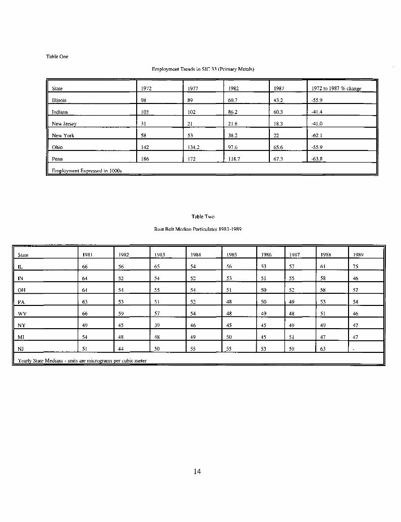
Table One

Employment Trends in SIC 33 (Primary Metals)

State

Illinois

Indiana

New Jersey

New York

Ohio

Penn

1972

98

103

31

58

142

186

1977

89

102

21

53

134.2

172

1982

60.7

86.2

21.6

38.2

97.6

118.7

1987

43.2

60.3

18.3

22

65.6

67.3

1972 to 1987 % change

-55.9

-41.4

-41.0

-62.1

-55.9

-63.8

Employment Expressed in 1000s

Table Two

Rust Belt Median Particulates 1981-1989

State

IL

IN

OH

PA

WV

NY

MI

NJ

1981

66

64

64

63

66

49

54

51

1982

56

52

54

53

59

45

48

44

1983

65

54

55

51

57

39

48

50

1984

54

52

54

52

54

46

49

55

1985

56

53

51

48

48

45

50

55

1986

53

51

50

50

49

45

45

53

1987

57

55

52

49

48

49

51

59

1988

61

58

58

53

51

49

47

63

1989

75

46

57

54

46

47

47

Yearly State Medians - units are micrograms per cubic meter

14

Table Three

Summary Statistics

Variable

mean participates

dummy fornon-attainment county

SIC 33Pre-1970

All Other Manufacturing employment

% of plants that employgreater than 100

Aggregate manufacturing employment

observations

1982 mean(SD)

52.0(15.5)

.64(.48)

.031(.056)

.34(.64)

.10(.06)

.38(.68)

1315

1987 mean(SD)

52.7(15.6)

.67(.47)

.019(.03)

.28(.53)

.10(.08)

.31(.56)

967

employment measured in 100,000s, the unit of analysis is a monitoring station in a county. Thus, counties with multiple monitoring stations aremore heavily represented. In 1982, mean particulates in attainment counties was 47 while in non-attainment counties it was 54.7.

15

Table Four

Paniculate Pollution by Two Digit SIC

SIC name and number

22 (Textile Mill)

23 (Apparel and Other Textiles)

24 (Lumber and Wood)

25 (Furniture and Fixtures)

26 (Paper)

27 (Printing and Publishing)

28 (Chemicals)

30 (Rubber and Plastics)

31 (Leather)

32 (Stone, Clay, glass)

33 (Primary Metals)

34 (Fabricated Metals)

35 (Industrial Machinery)

36 (Electronics)

37 (Transportation Equipment)

38 (Instruments)

39 (Misc.)

Pollution content for Two digit SIC

-.31

.088

-21.4**

-3.33*

-2.81*

-1.15

.37

-2.76*

-4.59

8.82**

1.79**

-.30

-.15

-1.41**

.58**

-.46**

-4.00*

Pollution content for all otherManufacturing employment

.000000109**

.000000104**

.000000287**

.000000173**

.000000205**

.000000257**

.0000000957**

.000000219*

.000000128**

.0000000367

.0000000159

.000000152*

.000000129

.000000252**

.0000000735**

.000000129**

.000000226**

MeanEmployment forthat Two DigitSIC

.003

.02

.003

.006

.012

.037

.018

.013

.002

.006

.031

.045

.056

.032

.036

.019

.008

correlationof all otherManufacturingemployment andemployment inthat SIC

.31

.53

.91

.85

.90

.95

.78

.92

.59

.67

.62

.96

.96

.92

.58

.48

.92

Each row of this table reports a separate regression where the dependent variable is the log of a monitoring station's yearly mean reading. This air quality measure isregressed on county manufacturing employment in a given two digit SIC indusry in 1982 and in the remaining SIC industries. Thus for each regression, I aggregate up allother industries employment to form aggregate manufacturing. This table reports the coefficient from the particulate regression and its statistical significance. ** indicates1% level, and * indicates 5% level. The third column reports the Two digit SIC mean county employment measured in 100,000 workers. The right column reports thecorrelation between each counties's two digit sic manufacturing employment and all other manufacturing employment in the county. N=1315.

16

Table Five

Rust Belt County Paniculate Levels Regressions

Dependent Variable is the log of a monitoring station's yearly average participates

Independentvariable Variable

county manufacturing in SIC 33 in Pre-1970Plants


total county manufacturing at allother plants

% of plants that employ greater than 100

% of plants that employ between 50 and 100

R2

observations

1982

AttainmentCounty

1.66(.22)

8.11(2.99)

.21(.04)

.19(.15)

-.29(.24)

.36

464

Non-AttainmentCounty

1.08(.39)

4.24(2.50)

-.05(.04)

-.20(.14)

.24(.41)

.21

851

1987

Attainment County

3.06(.71)

7.34(4.62)

.21(.09)

.11(-15)

.07(.50)

.21

294

Non-Attainment County

2.44(1.33)

1.09(2.42)

-.06(.07)

-.31(.17)

-.10(.63)

.17

646

(SIC 32 is Stone, Clay, Glass), SIC 33 is primary metals, standard errors in parentheses. Employment measured in 100,000s.

17

Table Six

Rust Belt County Particulate Levels Regressions

Dependent Variable is the log of a monitoring station's yearly average particulates



total county manufacturing at allother plants


constant

R2

observations

1982

AttainmentCounty

2.36(.22)

.21(.075)

.40(-14)

3.67(.04)

.21

464


1.34(.51)

.005(.03)

-.13(.31)

3.92(.04)

.25

851

1987

Attainment County

3.59(.41)

.19(.095)

.17(.11)

3.79(.04)

.14

294


2.64(1.30)

-.02(.06)

-.33(.12)

3.93(-02)

.12

646

SIC 33 is primary metals, standard errors in parentheses. Employment measured in 100,000s.

18

Table Seven

Aggregate Paniculate Levels Regressions

Dependent Variable is the log of a monitoring station's yearly average participates


Aggregate County ManufacturingEmployment


constant

R2

observations

1982

AttainmentCounty

.28(.09)

.41(.15)

3.71(.04)

.07

464


.07(.018)

-.18(.31)

3.94(.03)

.06

851

1987

Attainment County

.23(.10)

.10(.13)

3.82(.04)

.02

294


.09(.02)

-.38(.12)

3.94(.023)

.08

646

Standard errors are in parentheses. Employment measured in 100,000s.

19

Table Eight

Rust Belt County Paniculate Growth Rate Regression

The dependent variable is the growth rate between 1982 and 1987 in yearly average particulates at a given monitoring station.


change in county manufacturing in SIC 33 in Pre-1970Plants at the intensive margin

change in county manufacturing in SIC 33 in Pre-1970Plants at the extensive margin

change in all other county manufacturing at the intensivemargin

change in all other county manufacturing at the extensivemargin

constant

R2

observations

Attainment County

1.69(.64)

-8.12(5.17)

.58(.24)

.15(.19)

-.03(.014)

.04

246


1.97(.68)

-.67(.24)

.51(.35)

-.11(.07)

-.06(.014)

.03

560

Standard errors in parentheses. Manufacturing measured in 100,000s of jobs.

Table Nine

Willingess To Pay for Reduce Paniculate Levels

thoughtexperiment

particulates decline by 10

particulatesdecline by 10

particulates decline by 10

value of life

1,000,000

1,000,000

250,000

change inmortality rate fordemographic group

.0004

(men aged 45-64)

.00005(men aged 45)

.001men aged 65+

Risk Neutral WTP

400

50

258

Mortality rates for a given reduction in particulates are taken from Portney (1981). Risk Neutral willingness to pay (WTP) is calculated by multiplying thevalue of life by the change in the mortality rate.

20

1995-1996 Discussion Paper Series

Department of EconomicsColumbia University

1022 International Affairs Bldg.420 West 118th Street

New York, N.Y., 10027

The following papers are published in the 1995-96 Columbia University Discussion Paper serieswhich runs from early November to October 31 of the following year (Academic Year).

Domestic orders for discussion papers are available for purchase at the cost of $8.00 (U.S.) Perpaper and $140.00 (US) for the series.

Foreign orders cost $10.00 (US) per paper and $185.00 for the series.

To order discussion papers, please write to the Discussion Paper Coordinator at the above addressalong with a check for the appropriate amount, made payable to Department of Economics,Columbia University. Please be sure to include the series number of the requested paper when youplace an order.


9596-01 Protectionist Response to Import Competition in Declining Industries by: J. ChoiReconsidered

9596-02 New Estimates on Climate Demand: Evidence from Location Choice by: M. Cragg

M. Kahn

9596-03 Enforcement by Hearing by: C. Sanchirico

9596-04 Preferential Trading Areas and Multilateralism: Strangers, Friends or by: J. BhagwatiF o e s ? A. Panagariya

9596-05 Simplification, Progression and a Level Playing Field by: W. Vickrey

9596-06 The Burden of Proof in Civil Litigation by: C. Sanchirico

9596-07 Market Structure and the Timing of Technology Adoption

9596-08 The Emergence of the World Economy

9596-09 The Global Age: From a Skeptical South to a Fearful North

9596-10 A Conformity Test for Cointegration

9596-11 Identification and Kullback Information in the GLSEM

by: J. Choi

M. Thum

by: R. Findlay

by: J. Bhagwati

by: P. Dhrymes

by: P. Dhrymes

9596-12 Informational Leverage and the Endogenous Timing of ProductIntroductions

9596-13 Changes in Wage Inequality

9596-14 The Design of Monte Carlo Experiments for VAR Models

9596-15 A Toplogical Invariant for Competitive Markets

9596-16 Topology and Invertible Maps

9596-17 Smooth Infinite Economies

by: J. Choi

by: J. Mincer

by: P. Dhrymes

by: G. Chichilnisky

by: G. Chichilnisky

by: G. Chichilnisky


9596-18 Measuring Neighborhood Investments: Urban Quality of Life by: D. DipasqualeExpenditures by Race M

9596-19 The Silver Lining of Industrial Decline: Rust Belt Manufacturing's by: M. KahnImpact on Particulates

9596-20 Education's Role in Explaining Diabetic Health Investment Differentials by: M. Kahn

Documents

The Silver Lining of Industrial Decline: Rust Belt