The authors thank Ufuk Akcigit, Marco Bassetto, Pablo Fajgelbaum, Jeremy Greenwood, Berthold Herrendorf,

Tom Holmes, Alejandro Justiniano, Thomas Klier, Andrea Pozzi, Ed Prescott, Jim Schmitz, Todd Schoellman,

Marcelo Veracierto, Fabrizio Zilibotti, and seminar participants at Arizona State, Autonoma de Barcelona,

British Columbia, the Federal Reserve Banks of Chicago and St. Louis, Frankfurt, Notre Dame, Pennsylvania,

UCLA, Zurich, the 2012 Einaudi Roma Macro Junior conference, and the 2012 SED meetings (Cyprus) for

helpful comments. The authors thank Andrew Cole, Alex Hartman, Patrick Orr, Samin Peirovi, Billy Smith,

and especially Glenn Farley for excellent research assistance. The views expressed here are the authors’ and not

necessarily those of the Federal Reserve Bank of Atlanta or the Federal Reserve System. Any remaining errors

are the authors’ responsibility.

Please address questions regarding content to Simeon Alder, Notre Dame University, Department of Economics,

715 Flanner Hall, Notre Dame, Indiana 46556, 574-631-0373, simeon.alder.1@nd.edu; David Lagakos,

University of California, San Diego, Department of Economics 0508, 9500 Gilman Drive, La Jolla, California

92093-0508, lagakos@ucsd.edu; or Lee Ohanian, UCLA, Department of Economics, 405 Hilgard Avenue,

Los Angeles, California 90024, 310-825-0979, ohanian@econ.ucla.edu.

CQER Working Papers from the Federal Reserve Bank of Atlanta are available online at frbatlanta.org/frba/cqer/.

Subscribe online to receive e-mail notifications about new papers.

Center for Quantitative Economic Research WORKING PAPER SERIES

FEDERAL RESERVE BANK of ATLANTA

The Decline of the U.S. Rust Belt: A Macroeconomic Analysis

Simeon Alder, David Lagakos, and Lee Ohanian

CQER Working Paper 14-05

August 2014

Abstract: No region of the United States fared worse over the postwar period than the “Rust

Belt,” the heavy manufacturing zone bordering the Great Lakes. We argue that a lack of

competition in labor and output markets in the Rust Belt were responsible for much of the

region’s decline. We formalize this theory in a dynamic general-equilibrium model in which

productivity growth and regional employment shares are determined by the extent of

competition. When plausibly calibrated, the model explains roughly half the decline in the Rust

Belt’s manufacturing employment share. Industry evidence support the model’s predictions that

investment and productivity growth rates were relatively low in the Rust Belt.

JEL classification: E24, E65, J3, J5, L16, R13

Key words: Rust Belt, competition, productivity, unionization, monopoly

1. Introduction

No region of the United States fared worse over the post-war period than the area known as the

“Rust Belt.” While there is no official definition of the Rust Belt, it has come to mean the heavy

manufacturing zone bordering the Great Lakes, and including such cities as Detroit and Pittsburgh.

By any number of metrics, the Rust Belt’s share of aggregate economic activity declined dramati-

cally since the end of World War II.

We argue that the Rust Belt declined in large part due to a lackof competition in labor and output

markets in its most prominent industries, such as steel, automobile and rubber manufacturing.

The lack of competition in labor markets was closely linked to the behavior of powerful labor

unions that dominated the majority of the Rust Belt’s manufacturing industries. In output markets,

many of these same industries were run by a small set of oligopolists who, according to numerous

sources, actively stifled competition for decades after theend of WWII. We argue that this lack

of competition served to depress investment and productivity growth, which led to a movement of

economic activity out of the Rust Belt and into other parts ofthe country (notably the “Sun Belt”

in the U.S. South.)

We formalize the theory in a dynamic general-equilibrium model in which the extent of competi-

tion is what determines productivity growth. There is a continuum of goods in the economy, with

some fraction produced in the “Rust Belt” and the rest produced in the “Sun Belt.” The two regions

differ only in the extent of competition they face. Rust Beltproducers must hire workers through a

labor union that demands the competitive wage for each worker plus some fraction of the surplus

from production. Sun Belt producers pay only the competitive wage. In output markets, both re-

gions face a competitive fringe with whom they engage in Bertrand competition. We assume that

Rust Belt producers can “block” the fringe to some extent, while Sun Belt producers cannot. Firms

in both regions have the ability to undertake investment which, at a cost, increases the productivity

of any workers hired.

The main prediction of the theory is that the lesser the extent of competition in either labor or

output markets in the Rust Belt, the lower its investment andproductivity growth. We first illus-

trate this result qualitatively in a simple static version of the theory. We show there are two effects

which drive the theory’s prediction. The first effect is a hold-up problem which arises through the

collective bargaining process. Firms in both regions make costly investments to upgrade technol-

ogy. Unlike Sun Belt firms, however, Rust Belt firms must sharethe benefits from the technology

upgrade with the union. As a result, Rust Belt firms optimallychoose to invest less ex-ante than

they otherwise would. The second effect comes from differences in output market competition.

The inability of Sun Belt producers to block the competitivefringe gives them a stronger incentive

1

to invest in order to “escape the competition” (as in the workof Acemoglu and Akcigit(2011)

andAghion, Bloom, Blundell, Griffith, and Howitt(2005), among others.) This incentive is less

prevalent among Rust Belt producers, and hence they invest less.

We then embed this simple static framework in a richer dynamic model in which productivity

and the employment share in each region evolve endogenouslyover time. Because goods are

gross substitutes, employment and output tend to move to theregion with the highest productivity

growth, as in the model ofNgai and Pissarides(2007). The main quantitative experiment takes

the extent of competition over time as exogenous and computes the model’s predicted shares of

manufacturing employment in the Rust Belt. Discipline on the extent of competition over time

comes from estimates of the Rust Belt workers’ wage premiumsand from estimates of markups

in key Rust Belt industries. We find that the model explains roughly half the decline in the Rust

Belt’s manufacturing employment share.

We conclude by presenting several types of evidence supporting the theory’s predictions. First,

we show that investment and productivity growth in prominent Rust Belt industries were lower

than those of the rest of the economy, as predicted by the theory. Second, we present historical

evidence that productivity growth and technology adoptionrates for Rust Belt producers tended to

lag behind their foreign counterparts for much of the postwar period. Finally, we provide evidence

from the cross-section of metropolitan areas in the United States that the average wage premiums

paid to workers in 1950 – one sign of limited competition – arehighly negatively correlated with

employment growth from 1950 to 2000.

Our paper relates closely to a recent and growing literaturelinking competition and productivity.

As Holmes and Schmitz(2010), Syverson(2011) andSchmitz(2012) argue, there is now a sub-

stantial body of evidence linking greater competition to higher productivity. As one prominent

example,Schmitz(2005) shows that in the U.S. iron ore industry there were dramaticimprove-

ments in productivity following an increase in competitivepressure in the early 1980s, largely

due to efficiency gains made by incumbent producers. Similarly, Bloom, Draca, and Van Reenan

(2011) provide evidence that European firms most exposed to trade from China in recent years were

those that innovated more and saw larger increases in productivity. Pavcnik(2002) documents that

after the 1980s trade liberalization in Chile, the producers facing new import competition saw the

largest gains in productivity, in part because of efficiencyimprovements by existing producers. A

common theme with these papers and ours is that competition reduced rents to firms and workers

and forced them to improve productivity. Along these lines,our work also relates closely to that of

Cole and Ohanian(2004), who argue that policies that encouraged non-competitivebehavior in the

industrial sector during the Great Depression depressed aggregate economic activity even further.

From a modeling perspective, our work builds on several recent studies in which firms innovate in

2

order to “escape the competition,” such as the work ofAcemoglu and Akcigit(2011) andAghion,

Bloom, Blundell, Griffith, and Howitt(2005). The common theme is that greater competition in

output markets encourages incumbent firms to innovate more in order to maintain a productivity

advantage over potential entrants. Our model also relates to those ofParente and Prescott(1999)

andHerrendorf and Teixeira(2011), in which monopoly rights reduce productivity by encouraging

incumbent producers to block new technologies.

Our paper also complements the literature on the macroeconomic consequences of unionization.

The paper most related to ours in this literature is that ofHolmes(1998), who uses geographic

evidence along state borders to show that state policies favoring labor unions greatly depressed

manufacturing productivity over the postwar period. Our work also resembles that ofTaschereau-

Dumouchel(2012), who argues that even the threat of unionization can cause non-unionized firms

to distort their decisions so as to prevent unions from forming, and that ofBridgman(2011), who

argues that a union may rationally prefer inefficient production methods so long as competition is

sufficiently weak.1

To the best of our knowledge we are the first to explore the roleof competition in understanding

the Rust Belt’s decline. Our work contrasts with that ofYoon (2012), who argues that the Rust

Belt’s decline was due (in part) to rapid technological change in manufacturing, andGlaeser and

Ponzetto(2007), who argue that the declines in transportation costs eroded the Rust Belt’s natural

advantage in shipping goods via waterways. Our paper also differs from the work ofBlanchard

and Katz(1992) andFeyrer, Sacerdote, and Stern(2007), who study the long-term consequences

of the Rust Belt’s decline in employment (rather than the root causes of the decline.) Our model

is consistent with their finding that employment losses sustained by Rust Belt industries led to

population outflows rather than persistent increases in unemployment rates.

1While our model takes the extent of competition in labor markets as exogenous, several recent studies havemodeled the determinants of unionization in the United States over the last century.Dinlersoz and Greenwood(2012)argue that the rise of unions can be explained by technological change biased toward the unskilled, which increasedthe benefits of their forming a union, while the later fall of unions can be explained by technological change biasedtoward machines. Relatedly,Acikgoz and Kaymak(2012) argue that the fall of unionization was due instead to therising skill premium, caused (perhaps) by skill-biased technological change. A common theme in these papers, as wellas other papers in the literature, such as that ofBorjas and Ramey(1995) and that ofTaschereau-Dumouchel(2012),is the link between inequality and unionization, which is absent from the current paper.

3

2. Decline of the Rust Belt

In this section we present the basic fact to be explained: thedecline of the Rust Belt. We show

that, by a number of metrics, the Rust Belt’s share of aggregate economic activity fell substantially

over the post-war period.

2.1. Our Definition of the Rust Belt

While there is no widely agreed upon definition, most users ofthe term “Rust Belt” use it to refer

to the heavy manufacturing area bordering the Great Lakes (see e.g.Blanchard and Katz(1992)

andFeyrer, Sacerdote, and Stern(2007) and the references therein.) For the purposes of this paper,

we define the Rust Belt to be the region encompassing Illinois, Indiana, Michigan, New York,

Ohio, Pennsylvania, West Virginia and Wisconsin. This definition keeps the essence of previous

use of the term and, in addition, allows us to aggregate various data sources in a consistent way.

2.2. Measuring the Decline

Our main source of data are the decadal U.S. Censuses of 1950 through 2000, available through

the Integrated Public Use Microdata Series (IPUMS). The only sample restriction is to focus only

on private-sector workers who are not primarily self-employed. We also draw on state-level em-

ployment data from 1970 and onward from the U.S. Bureau of Economic Analysis (BEA), and

state-level value added and wage data from 1963 and onward, also from the BEA.

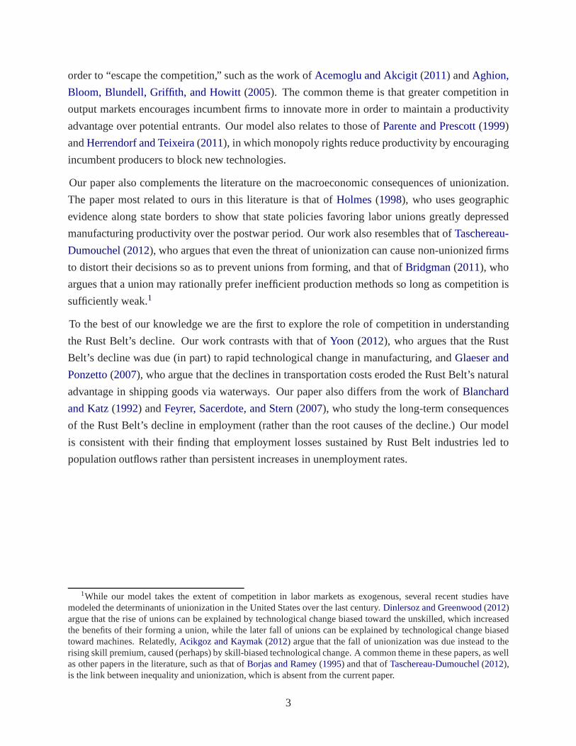
Figure 1 plots the Rust Belt’s share of aggregate employment (grey dashed line) and share of

manufacturing employment (solid black line). Both time series consist of estimates from the census

data for 1950 and 1960 plus BEA state-level data in subsequent years (the census and BEA provide

almost identical estimates in overlapping years). The figure shows that, by both metrics, the Rust

Belt’s share declined dramatically. The Rust Belt employed43 percent of aggregate employment in

1950, and just 27 percent in 2000. In terms of manufacturing employment, the Rust Belt share was

over one-half in 1950 and fell to one-third in 2000. Notably,the decline is much more dramatic

from 1950 to 1980 than since 1980, in which the Rust Belt’s shares of aggregate and manufacturing

employment declined by only a few percentage points.

The fact that the Rust Belt’s share of manufacturing employment dropped by so much suggests

that the decline of the Rust Belt is not a simple story about structural change. That is, the Rust

Belt’s decline was not simply because the United States’ manufacturing sector declined, and the

Rust Belt happened to be intensive in manufacturing. The solid black line in Figure1 clearly shows

that the Rust Belt’s share of employment declinedeven within the manufacturing sector. Figure5,

in the Appendix, shows that in absolute levels, manufacturing employment in the Rust Belt stayed

4

0.25

0.30

0.35

0.40

0.45

0.50

0.55

Fra

ctio

n in

Rus

t Bel

t

1950 1960 1970 1980 1990 2000year

Aggregate Employment Manufacturing Employment

Figure 1: Fraction of Employment and Manufacturing Employment in the Rust Belt

roughly constant over this period while manufacturing employment outside the Rust Belt roughly

doubled. What happened, according to these figures, is that manufacturing employment moved

from the Rust Belt to elsewhere in the country.

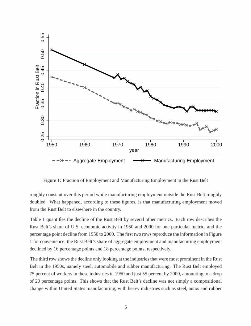
Table1 quantifies the decline of the Rust Belt by several other metrics. Each row describes the

Rust Belt’s share of U.S. economic activity in 1950 and 2000 for one particular metric, and the

percentage point decline from 1950 to 2000. The first two rowsreproduce the information in Figure

1 for convenience; the Rust Belt’s share of aggregate employment and manufacturing employment

declined by 16 percentage points and 18 percentage points, respectively.

The third row shows the decline only looking at the industries that were most prominent in the Rust

Belt in the 1950s, namely steel, automobile and rubber manufacturing. The Rust Belt employed

75 percent of workers in these industries in 1950 and just 55 percent by 2000, amounting to a drop

of 20 percentage points. This shows that the Rust Belt’s decline was not simply a compositional

change within United States manufacturing, with heavy industries such as steel, autos and rubber

5

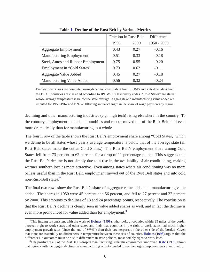
Table 1: Decline of the Rust Belt by Various Metrics

Fraction in Rust Belt Difference

1950 2000 1950 - 2000

Aggregate Employment 0.43 0.27 -0.16

Manufacturing Employment 0.51 0.33 -0.18

Steel, Autos and Rubber Employment 0.75 0.55 -0.20

Employment in “Cold States” 0.73 0.62 -0.11

Aggregate Value Added 0.45 0.27 -0.18

Manufacturing Value Added 0.56 0.32 -0.24

Employment shares are computed using decennial census datafrom IPUMS and state-level data from

the BEA. Industries are classified according to IPUMS 1990 industry codes. “Cold States” are states

whose average temperature is below the state average. Aggregate and manufacturing value added are

imputed for 1950-1962 and 1997-2000 using annual changes inthe share of wage payments by region.

declining and other manufacturing industries (e.g. high tech) rising elsewhere in the country. To

the contrary, employment in steel, automobiles and rubber moved out of the Rust Belt, and even

more dramatically than for manufacturing as a whole.

The fourth row of the table shows the Rust Belt’s employment share among “Cold States,” which

we define to be all states whose yearly average temperature isbelow that of the average state (all

Rust Belt states make the cut as Cold States.) The Rust Belt’semployment share among Cold

States fell from 73 percent to 62 percent, for a drop of 11 percentage points. This suggests that

the Rust Belt’s decline is not simply due to a rise in the availability of air conditioning, making

warmer southern locales more attractive. Even among stateswhere air conditioning was no more

or less useful than in the Rust Belt, employment moved out of the Rust Belt states and into cold

non-Rust-Belt states.2

The final two rows show the Rust Belt’s share of aggregate value added and manufacturing value

added. The shares in 1950 were 45 percent and 56 percent, and fell to 27 percent and 32 percent

by 2000. This amounts to declines of 18 and 24 percentage points, respecitvely. The conclusion is

that the Rust Belt’s decline is clearly seen in value added shares as well, and in fact the decline is

even more pronounced for value added than for employment.3

2This finding is consistent with the work ofHolmes(1998), who looks at counties within 25 miles of the borderbetween right-to-work states and other states and finds thatcountries in the right-to-work states had much higheremployment growth rates (since the end of WWII) than their counterparts on the other side of the border. Giventhat there are essentially no differences in temperature between these sets of counties,Holmes(1998) argues that thedifferences in outcomes must be due to differences in state policies, most notably right-to-work laws.

3One positive result of the Rust Belt’s drop in manufacturingis that the environment improved.Kahn(1999) showsthat regions with the biggest declines in manufacturing activity tended to see the largest improvements in air quality.

6

3. Lack of Competition in the Rust Belt

In this section we show that one salient characteristic of the Rust Belt was a relatively low degree

of competition in labor and output and markets for several decades after the end of WWII. Labor

markets in the Rust Belt were dominated by powerful labor unions in most of the prominent Rust

Belt industries. Output markets were characterized by close-knit oligopolists in many industries

that, by many metrics, faced very low competitive pressure from the outside. Around the 1980s,

however, competitive pressure increased, as output markets drew new competition from abroad

and new entrants at home, and labor markets witnessed a drop in the influence of unions.

3.1. Lack of Competition in Labor Markets

It is widely known that unions dominated labor markets in many Rust Belt manufacturing indus-

tries. The two largest and most powerful unions in the UnitedStates at the time were the United

Steelworkers (USW) and United Auto Workers (UAW). Roughly two thirds of all auto workers

were members of the UAW, while an only slighter smaller fraction of steel workers were mem-

bers of the USW.4 The majority of steel and auto workers were employed in the Rust Belt for

decades after the end of WWII. According to the U.S. Bureau ofLabor Statistics, of the top ten

most unionized states in 1974, seven were Rust Belt states, as were four of the top five (Michigan,

West Virginia, New York and Pennsylvania.)5

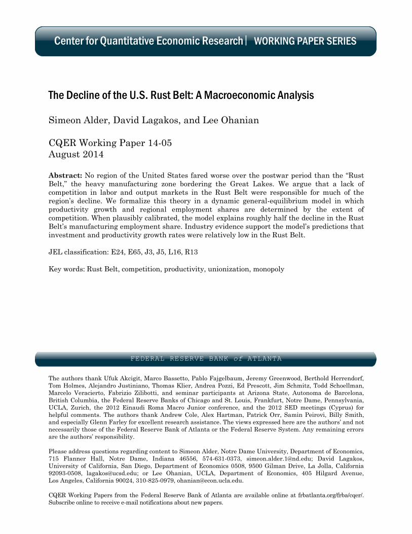
It is also well established that these unions extracted great concessions from their employers and

enjoyed substantial rents. Figure2 shows one simple metric of these rents: the ratio of average

wages in the Rust Belt to average wages in the rest of the country. The dashed gray line shows the

relative wages for all workers, and the solid black line shows the relative wages for manufacturing

workers. From 1950 to 1980 the average wage was at least 10 percent higher in the Rust Belt than

in the rest of the country, and reached 15 percent (among manufacturing workers) by 1980.6

Industry histories provide more direct evidence of the types of rents enjoyed by workers in these

unions. Ingrassia(2011) andVlasic (2011) provide numerous examples of various concessions

extracted from the “Big Three” auto producers of Ford, General Motors and Chrysler from WWII.

By 1973, a UAW worker could earn “princely sums” working on production or other union-created

4These figures are for 1970 and come from BLS Bulletin 1937 Appendix D. The UAW and USW also had largemembership rates in a diverse set of other manufacturing industries (Goldfield, 1987).

5BLS Bulletin 1865 and BLS Bulletin 1370-12. Unionization rate are the percent of all non-agricultural employ-ment that is covered under a collective bargaining agreement.

6The ratio of average wages, while a crude measure of wage premiums, is similar to the estimated “Rust Belt”dummy we find when regressing individual-level wages on education, potential experience and other controls. Moregenerally, the ratio of average wages is in the same range as the estimated union wage premium documented in a longliterature (see e.g.Blanchflower and Bryson(2004) for a review.)

7

1.00

1.05

1.10

1.15

1.20

Rel

tive

Wag

es in

Rus

t Bel

t

1950 1960 1970 1980 1990 2000year

All Workers Manufacturing Workers

Figure 2: Relative Wages of Rust Belt Workers

jobs, such as serving on the plant “recreation committee.” In many cases workers could retire with

full benefits as early as age 48 (Ingrassia, 2011, pp. 46, 56). In steel,Tiffany (1988) states that

in 1959, average hourly earnings for steel workers were morethan 40 percent higher than the

all-manufacturing average in the United States, and pointsto this premium as evidence that steel

workers earned rents (p. 178). Evidence of non-wage rents insteel abound, such as clauses in

various steelworker contracts that guaranteed that the steel mills would be shut down on the first

day of deer hunting season (see e.g.Hoerr(1988)).

Figure2 also provides an indication that union power began to decline during the 1980s. Relative

wages in the Rust Belt fell from roughly 12 percent above other workers to just 4 percent above

by 2000. Not coincidentally, union membership dropped steadily over this period. Figure6 (in the

Appendix) shows the unionization rate for the country as a whole using data fromGoldfield(1987),

and in the Rust Belt, using the state-level unionization database ofHirsch and Macpherson(2003)).

In 1980, the first year of available disaggregated data, 30 percent of the Rust Belt workforce was

unionized. By 2000, the unionization rate in the Rust Belt was below 20 percent.

8

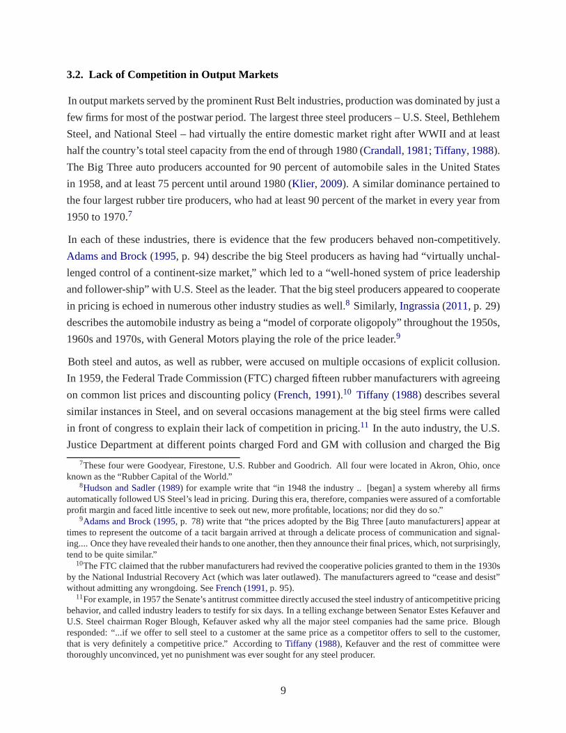
3.2. Lack of Competition in Output Markets

In output markets served by the prominent Rust Belt industries, production was dominated by just a

few firms for most of the postwar period. The largest three steel producers – U.S. Steel, Bethlehem

Steel, and National Steel – had virtually the entire domestic market right after WWII and at least

half the country’s total steel capacity from the end of through 1980 (Crandall, 1981; Tiffany, 1988).

The Big Three auto producers accounted for 90 percent of automobile sales in the United States

in 1958, and at least 75 percent until around 1980 (Klier, 2009). A similar dominance pertained to

the four largest rubber tire producers, who had at least 90 percent of the market in every year from

1950 to 1970.7

In each of these industries, there is evidence that the few producers behaved non-competitively.

Adams and Brock(1995, p. 94) describe the big Steel producers as having had “virtually unchal-

lenged control of a continent-size market,” which led to a “well-honed system of price leadership

and follower-ship” with U.S. Steel as the leader. That the big steel producers appeared to cooperate

in pricing is echoed in numerous other industry studies as well.8 Similarly, Ingrassia(2011, p. 29)

describes the automobile industry as being a “model of corporate oligopoly” throughout the 1950s,

1960s and 1970s, with General Motors playing the role of the price leader.9

Both steel and autos, as well as rubber, were accused on multiple occasions of explicit collusion.

In 1959, the Federal Trade Commission (FTC) charged fifteen rubber manufacturers with agreeing

on common list prices and discounting policy (French, 1991).10 Tiffany (1988) describes several

similar instances in Steel, and on several occasions management at the big steel firms were called

in front of congress to explain their lack of competition in pricing.11 In the auto industry, the U.S.

Justice Department at different points charged Ford and GM with collusion and charged the Big

7These four were Goodyear, Firestone, U.S. Rubber and Goodrich. All four were located in Akron, Ohio, onceknown as the “Rubber Capital of the World.”

8Hudson and Sadler(1989) for example write that “in 1948 the industry .. [began] a system whereby all firmsautomatically followed US Steel’s lead in pricing. During this era, therefore, companies were assured of a comfortableprofit margin and faced little incentive to seek out new, moreprofitable, locations; nor did they do so.”

9Adams and Brock(1995, p. 78) write that “the prices adopted by the Big Three [auto manufacturers] appear attimes to represent the outcome of a tacit bargain arrived at through a delicate process of communication and signal-ing.... Once they have revealed their hands to one another, then they announce their final prices, which, not surprisingly,tend to be quite similar.”

10The FTC claimed that the rubber manufacturers had revived the cooperative policies granted to them in the 1930sby the National Industrial Recovery Act (which was later outlawed). The manufacturers agreed to “cease and desist”without admitting any wrongdoing. SeeFrench(1991, p. 95).

11For example, in 1957 the Senate’s antitrust committee directly accused the steel industry of anticompetitive pricingbehavior, and called industry leaders to testify for six days. In a telling exchange between Senator Estes Kefauver andU.S. Steel chairman Roger Blough, Kefauver asked why all themajor steel companies had the same price. Bloughresponded: “...if we offer to sell steel to a customer at the same price as a competitor offers to sell to the customer,that is very definitely a competitive price.” According toTiffany (1988), Kefauver and the rest of committee werethoroughly unconvinced, yet no punishment was ever sought for any steel producer.

9

Three with conspiring to eliminate competition (Adams and Brock, 1995, p. 87).

Several types of evidence suggest that competitive pressure picked up starting in the 1970s and

1980s, as the cost of imports from abroad plummeted and new firms entered the domestic markets

for goods formerly supplied almost exclusively by Rust Beltproducers. In each of the steel, auto

and rubber industries, concentration ratios fell substantially starting in the 1970s and 1980s. In

autos, the Big Three’ currently have less than half the domestic market, with even lower figures

in steel and rubber (Tiffany, 1988; French, 1991). Estimates of markups paint a similar picture,

at least where such estimates exist. In the steel industry,Collard-Wexler and De Loecker(2012)

estimate markups of on average 25 percent over the period 1967 through 1987 for the integrated

segment of the steel industry (most of which was in the Rust Belt).12 In the period since 1987 their

estimated markups averaged just 13 percent.13

4. Simple Model

In this section we present a simple model which illustrates the main components of the theory.

The model links the extent of competition in labor and outputmarkets to investment and hence

productivity growth. The model predicts that less competition in either market leads to lower

investment.

4.1. Environment

There is a continuum of intermediates, indexed byj, which are combined to produce a final good.

The production function for the final good is given by

Y =

(

∫ 1

0y( j)

12di

)2

(1)

where any two intermediates have elasticity of substitution two between them. The final good can

either be consumed or used for investment. Intermediatesj ∈ [0, 12) are produced in the “Rust Belt,”

and intermediatesj ∈ [12,1] are produced in the “Sun Belt.” The two regions differ in the nature of

their competition in labor markets and output markets (described below). Each intermediatej is

produced in an industry that has a single “leader” firm and, inthe Sun Belt region, a competitive

12These numbers are consistent with estimated markups in the auto industry over this period.Berndt, Friedlaender,and Chiang(1990) estimate markups for Ford, GM and Chrysler over the period 1959 through 1983. Taking an averageof the three firms and the years in their sample, their estimated markups are 21 percent.

13The evidence ofSchmitz(2005) andDunne, Klimek, and Schmitz(2010) shows that the early 1980s were a timewhen competitive pressure in the United States increased substantially in at least two important industries: iron oreand cement. In both industries one impetus for the increasedcompetition was a lowering of transportation costs forforeign competitors.

10

fringe (also described below).

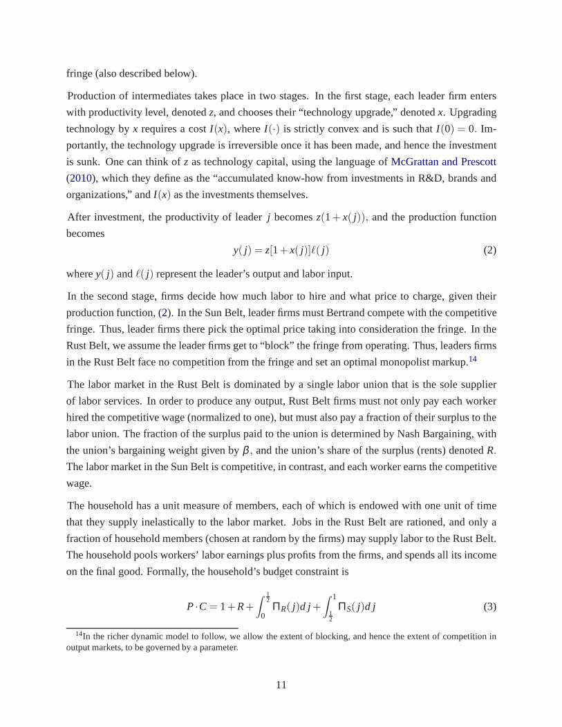
Production of intermediates takes place in two stages. In the first stage, each leader firm enters

with productivity level, denotedz, and chooses their “technology upgrade,” denotedx. Upgrading

technology byx requires a costI(x), whereI(·) is strictly convex and is such thatI(0) = 0. Im-

portantly, the technology upgrade is irreversible once it has been made, and hence the investment

is sunk. One can think ofz as technology capital, using the language ofMcGrattan and Prescott

(2010), which they define as the “accumulated know-how from investments in R&D, brands and

organizations,” andI(x) as the investments themselves.

After investment, the productivity of leaderj becomesz(1+ x( j)), and the production function

becomes

y( j) = z[1+x( j)]ℓ( j) (2)

wherey( j) andℓ( j) represent the leader’s output and labor input.

In the second stage, firms decide how much labor to hire and what price to charge, given their

production function, (2). In the Sun Belt, leader firms must Bertrand compete with thecompetitive

fringe. Thus, leader firms there pick the optimal price taking into consideration the fringe. In the

Rust Belt, we assume the leader firms get to “block” the fringefrom operating. Thus, leaders firms

in the Rust Belt face no competition from the fringe and set anoptimal monopolist markup.14

The labor market in the Rust Belt is dominated by a single labor union that is the sole supplier

of labor services. In order to produce any output, Rust Belt firms must not only pay each worker

hired the competitive wage (normalized to one), but must also pay a fraction of their surplus to the

labor union. The fraction of the surplus paid to the union is determined by Nash Bargaining, with

the union’s bargaining weight given byβ , and the union’s share of the surplus (rents) denotedR.

The labor market in the Sun Belt is competitive, in contrast,and each worker earns the competitive

wage.

The household has a unit measure of members, each of which is endowed with one unit of time

that they supply inelastically to the labor market. Jobs in the Rust Belt are rationed, and only a

fraction of household members (chosen at random by the firms)may supply labor to the Rust Belt.

The household pools workers’ labor earnings plus profits from the firms, and spends all its income

on the final good. Formally, the household’s budget constraint is

P ·C= 1+R+∫ 1

2

0ΠR( j)d j+

∫ 1

12

ΠS( j)d j (3)

14In the richer dynamic model to follow, we allow the extent of blocking, and hence the extent of competition inoutput markets, to be governed by a parameter.

11

whereP is the price of the final good,C is the quantity of the final good purchased for consumption,

1+R is the labor earnings plus the rents earned by workers in the Rust Belt, andΠR( j) andΠS( j)

are profits earned by intermediate firms in the Rust Belt and Sun Belt.

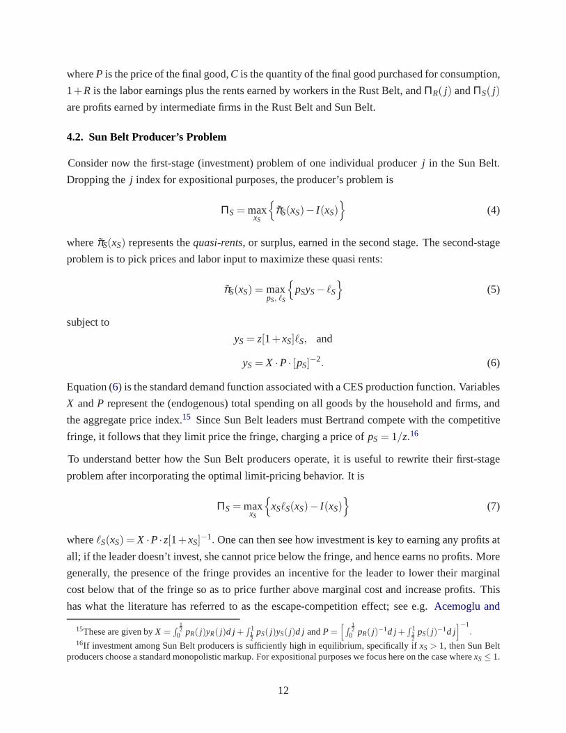
4.2. Sun Belt Producer’s Problem

Consider now the first-stage (investment) problem of one individual producerj in the Sun Belt.

Dropping thej index for expositional purposes, the producer’s problem is

ΠS= maxxS

{

π̃S(xS)− I(xS)}

(4)

whereπ̃S(xS) represents thequasi-rents, or surplus, earned in the second stage. The second-stage

problem is to pick prices and labor input to maximize these quasi rents:

π̃S(xS) = maxpS, ℓS

{

pSyS− ℓS

}

(5)

subject to

yS= z[1+xS]ℓS, and

yS= X ·P · [pS]−2. (6)

Equation (6) is the standard demand function associated with a CES production function. Variables

X andP represent the (endogenous) total spending on all goods by the household and firms, and

the aggregate price index.15 Since Sun Belt leaders must Bertrand compete with the competitive

fringe, it follows that they limit price the fringe, charging a price ofpS= 1/z.16

To understand better how the Sun Belt producers operate, it is useful to rewrite their first-stage

problem after incorporating the optimal limit-pricing behavior. It is

ΠS= maxxS

{

xSℓS(xS)− I(xS)}

(7)

whereℓS(xS) = X ·P·z[1+xS]−1. One can then see how investment is key to earning any profits at

all; if the leader doesn’t invest, she cannot price below thefringe, and hence earns no profits. More

generally, the presence of the fringe provides an incentivefor the leader to lower their marginal

cost below that of the fringe so as to price further above marginal cost and increase profits. This

has what the literature has referred to as the escape-competition effect; see e.g.Acemoglu and

15These are given byX =∫

12

0 pR( j)yR( j)d j+∫ 1

12

pS( j)yS( j)d j andP=[

∫

12

0 pR( j)−1d j+∫ 1

12

pS( j)−1d j]−1

.16If investment among Sun Belt producers is sufficiently high in equilibrium, specifically ifxS > 1, then Sun Belt

producers choose a standard monopolistic markup. For expositional purposes we focus here on the case wherexS≤ 1.

12

Akcigit (2011) andAghion, Bloom, Blundell, Griffith, and Howitt(2005).

4.3. Rust Belt Producer’s Problem

The Rust Belt producers’ problem differs from the Sun Belt producers’ problem in two ways. First,

in output markets, the Rust Belt gets to block the competitive fringe and set a standard monopolist

markup. Second, in labor markets, the Rust Belt must hire labor through a union with collective

bargaining rights. The union supplies labor in exchange forthe competitive wage plus a share of

the firms’ surplus after producing.

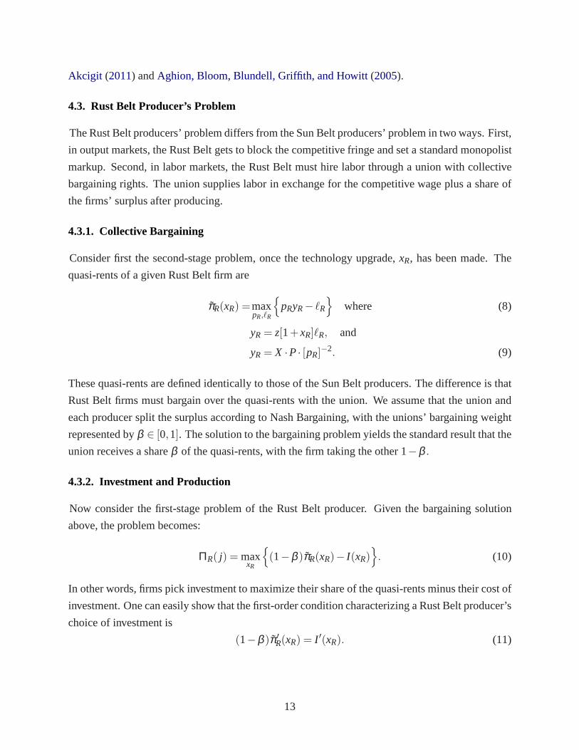
4.3.1. Collective Bargaining

Consider first the second-stage problem, once the technology upgrade,xR, has been made. The

quasi-rents of a given Rust Belt firm are

π̃R(xR) =maxpR,ℓR

{

pRyR− ℓR

}

where (8)

yR = z[1+xR]ℓR, and

yR = X ·P· [pR]−2. (9)

These quasi-rents are defined identically to those of the SunBelt producers. The difference is that

Rust Belt firms must bargain over the quasi-rents with the union. We assume that the union and

each producer split the surplus according to Nash Bargaining, with the unions’ bargaining weight

represented byβ ∈ [0,1]. The solution to the bargaining problem yields the standardresult that the

union receives a shareβ of the quasi-rents, with the firm taking the other 1−β .

4.3.2. Investment and Production

Now consider the first-stage problem of the Rust Belt producer. Given the bargaining solution

above, the problem becomes:

ΠR( j) = maxxR

{

(1−β )π̃R(xR)− I(xR)}

. (10)

In other words, firms pick investment to maximize their shareof the quasi-rents minus their cost of

investment. One can easily show that the first-order condition characterizing a Rust Belt producer’s

choice of investment is

(1−β )π̃ ′R(xR) = I ′(xR). (11)

13

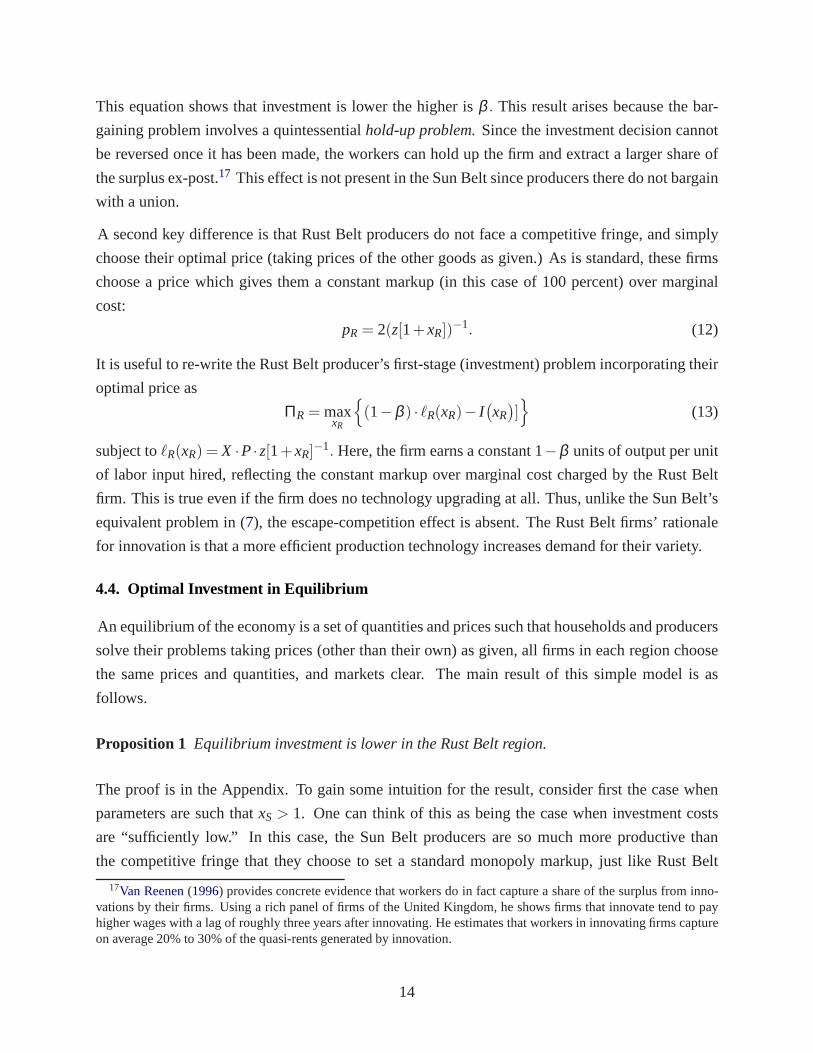
This equation shows that investment is lower the higher isβ . This result arises because the bar-

gaining problem involves a quintessentialhold-up problem.Since the investment decision cannot

be reversed once it has been made, the workers can hold up the firm and extract a larger share of

the surplus ex-post.17 This effect is not present in the Sun Belt since producers there do not bargain

with a union.

A second key difference is that Rust Belt producers do not face a competitive fringe, and simply

choose their optimal price (taking prices of the other goodsas given.) As is standard, these firms

choose a price which gives them a constant markup (in this case of 100 percent) over marginal

cost:

pR = 2(z[1+xR])−1. (12)

It is useful to re-write the Rust Belt producer’s first-stage(investment) problem incorporating their

optimal price as

ΠR= maxxR

{

(1−β ) · ℓR(xR)− I(

xR)

]}

(13)

subject toℓR(xR) = X ·P·z[1+xR]−1. Here, the firm earns a constant 1−β units of output per unit

of labor input hired, reflecting the constant markup over marginal cost charged by the Rust Belt

firm. This is true even if the firm does no technology upgradingat all. Thus, unlike the Sun Belt’s

equivalent problem in (7), the escape-competition effect is absent. The Rust Belt firms’ rationale

for innovation is that a more efficient production technology increases demand for their variety.

4.4. Optimal Investment in Equilibrium

An equilibrium of the economy is a set of quantities and prices such that households and producers

solve their problems taking prices (other than their own) asgiven, all firms in each region choose

the same prices and quantities, and markets clear. The main result of this simple model is as

follows.

Proposition 1 Equilibrium investment is lower in the Rust Belt region.

The proof is in the Appendix. To gain some intuition for the result, consider first the case when

parameters are such thatxS > 1. One can think of this as being the case when investment costs

are “sufficiently low.” In this case, the Sun Belt producers are so much more productive than

the competitive fringe that they choose to set a standard monopoly markup, just like Rust Belt

17Van Reenen(1996) provides concrete evidence that workers do in fact capturea share of the surplus from inno-vations by their firms. Using a rich panel of firms of the UnitedKingdom, he shows firms that innovate tend to payhigher wages with a lag of roughly three years after innovating. He estimates that workers in innovating firms captureon average 20% to 30% of the quasi-rents generated by innovation.

14

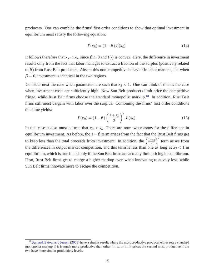
producers. One can combine the firms’ first order conditions to show that optimal investment in

equilibrium must satisfy the following equation:

I ′(xR) = (1−β ) I ′(xS). (14)

It follows therefore thatxR< xS, sinceβ > 0 andI(·) is convex. Here, the difference in investment

results only from the fact that labor manages to extract a fraction of the surplus (positively related

to β ) from Rust Belt producers. Absent this non-competitive behavior in labor markets, i.e. when

β = 0, investment is identical in the two regions.

Consider next the case when parameters are such thatxS < 1. One can think of this as the case

when investment costs are sufficiently high. Now Sun Belt producers limit price the competitive

fringe, while Rust Belt firms choose the standard monopolistmarkup.18 In addition, Rust Belt

firms still must bargain with labor over the surplus. Combining the firms’ first order conditions

this time yields:

I ′(xR) = (1−β )(

1+xS

2

)2

I ′(xS). (15)

In this case it also must be true thatxR < xS. There are now two reasons for the difference in

equilibrium investment. As before, the 1−β term arises from the fact that the Rust Belt firms get

to keep less than the total proceeds from investment. In addition, the(

1+xS2

)2term arises from

the differences in output market competition, and this termis less than one as long asxS < 1 in

equilibrium, which is true if and only if the Sun Belt firms areactually limit pricing in equilibrium.

If so, Rust Belt firms get to charge a higher markup even when innovating relatively less, while

Sun Belt firms innovate more to escape the competition.

18Bernard, Eaton, and Jensen(2003) have a similar result, where the most productive producer either sets a standardmonopolist markup if it is much more productive than other firms, or limit prices the second most productive if thetwo have more similar productivty levels.

15

5. Dynamic Model

We now embed the main features of the simple static model intoa richer dynamic model that

can be used for quantitative experiments. The dynamic modeldiffers in several main ways from

the static model. First, firm productivity and employment shares by region evolve endogenously

over time. Second, the extent of output-market competitionis governed by a parameter, which

allows more flexibly in the quantitative work. Third, the extent of competition in output markets

is determined not just by the escape-competition effect, but by an opposingSchumpeterian effect,

which has been emphasized by the literature. Thus, whether greater competition in output markets

leads to lower or higher investment in equilibrium is not predetermined in the model, but rather

driven by the data used to discipline the model.

5.1. Environment

Preferences of the household are given by

U =∞

∑t=0

δ tCt , (16)

whereδ is the discount factor andCt is consumption of a final good. The final good is produced

using the CES production function

Yt =

(

∫ 1

0qt( j)

σ−1σ d j

)σ

σ−1

, (17)

whereσ is the elasticity of substitution between any pair of intermediates in the economy. We

assume thatσ > 1, which implies that the intermediates are gross substitutes. As before, the final

good can be used for both consumption and investment, and each intermediate is produced by a

single producer located in one of two regions: the Rust Belt and the Sun Belt. The measure of

goods produced in the Rust Belt isλ ∈ (0,1), while the measure of goods produced in the Sun Belt

is 1−λ . Just as in the simple model, the production of each good requires a single input, labor,

and the wage is normalized to unity each period.

Each period is divided into two stages. In the first stage, theintermediate firms decide how much

to upgrade their technology, denoted byxt . In the second stage, the firms decide how much labor

to hire and what price to charge, and then produce. As before,Rust Belt producers bargain with

unions over their surplus after producing, with bargainingweightβt for the union and 1−βt for

the firm. Note that the bargaining weight may change over time, as thet subscripts indicate.

Producers in both regions face a competitive fringe each period. In the Sun Belt, the fringe enters

16

with productivity φzS,t , wherezS,t is the initial productivity among Sun Belt producers, and the

parameterφ > 0 governs how effectively the fringe catches up to the leaderfirms each period. In

the Rust Belt, the fringe begins the second stage with productivity φzR,t(1− µt). The parameter

µt stands for the extent of “monopoly power” in output markets,and captures the ease with which

incumbents can block entry by potential challengers. Asµt goes to one, the extent of output-

market competition in the Rust Belt is minimized, as in the simple model. Asµt goes to zero,

imperfections in output market vanish, as in the Sun Belt. One can think ofµt as arising from

policies which protect incumbent producers, such as emphasized byParente and Prescott(1999)

andHerrendorf and Teixeira(2011), though we interpret the extent of competition broadly as any

reason the leaders would face immediate competitors with high costs.

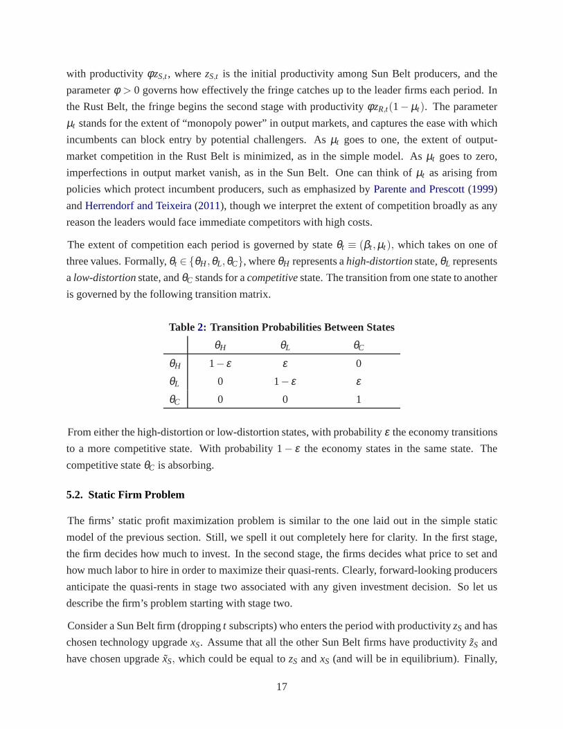
The extent of competition each period is governed by stateθt ≡ (βt,µt), which takes on one of

three values. Formally,θt ∈ {θH ,θL,θC}, whereθH represents ahigh-distortionstate,θL represents

a low-distortionstate, andθC stands for acompetitivestate. The transition from one state to another

is governed by the following transition matrix.

Table 2: Transition Probabilities Between States

θH θL θC

θH 1− ε ε 0

θL 0 1− ε εθC 0 0 1

From either the high-distortion or low-distortion states,with probabilityε the economy transitions

to a more competitive state. With probability 1− ε the economy states in the same state. The

competitive stateθC is absorbing.

5.2. Static Firm Problem

The firms’ static profit maximization problem is similar to the one laid out in the simple static

model of the previous section. Still, we spell it out completely here for clarity. In the first stage,

the firm decides how much to invest. In the second stage, the firms decides what price to set and

how much labor to hire in order to maximize their quasi-rents. Clearly, forward-looking producers

anticipate the quasi-rents in stage two associated with anygiven investment decision. So let us

describe the firm’s problem starting with stage two.

Consider a Sun Belt firm (droppingt subscripts) who enters the period with productivityzS and has

chosen technology upgradexS. Assume that all the other Sun Belt firms have productivity ˜zS and

have chosen upgrade ˜xS, which could be equal tozS andxS (and will be in equilibrium). Finally,

17

assume that all Rust Belt producers have productivity ˜zR and have chosen ˜xR. To keep the notation

tidy, we defineZS ≡ (zS, z̃S, z̃R) andXS ≡ (xS, x̃S, x̃R). Whenever possible, we also drop the firm

label j ∈ [0,1]. The static profit maximization problem of the Run Belt firm isto maximize the

quasi-rents:

π̃S(ZS,XS;θ) = maxpS, ℓS

{

pSyS− ℓS

}

(18)

subject toyS= zS[1+xS]ℓS andyS=X ·Pσ−1 · p−σS , which are the production function and standard

demand function under CES preferences. As before,X andP represent total spending on all goods

by the household and the aggregate price index, respectively:

X =

∫ λ

0pR( j)qR( j)d j+

∫ 1

λpS( j)qS( j)d j

P=[

∫ λ

0pR( j)1−σ d j+

∫ 1

λpS( j)1−σ d j

]1

1−σ.

Since Sun Belt leaders must Bertrand compete with the competitive fringe, it follows that they

limit price the fringe and chargepS(i) =1

φzS.19

Now consider a Rust Belt firm who enters the period with productivity zR and has chosen invest-

ment levelxR, while all other Rust Belt producers have productivity ˜zR and investment ˜xR. Assume

that all Sun Belt producers have productivity ˜zS and have chosen investment ˜xS. As we did for the

Sun Belt, let us defineZR≡ (zR, z̃R, z̃S) andXR≡ (xR, x̃R, x̃S). Quasi-rents of the Rust Belt are given

by

π̃R(ZR,XR;θ) = maxpR, ℓR

{

pRyR− ℓR

}

(19)

subject toyR = zR[1+ xR]ℓR andyR = X ·Pσ−1 · p−σR . The additional argument in the Rust Belt

producer’s profit function,µ, reflects the difference in the limit price compared to a Sun Belt

producer.

5.3. Dynamic Firm Problem

We now consider the dynamic problem of the firms. The Bellman equation that describes a Sun

Belt producer’s problem is:

VS(ZS;θ) = maxxS

{

π̃S(ZS,XS)− I(xS,ZS)+δE[

VS(

ZS;θ ′)

]}

(20)

19For expositional purposes we focus on the case where investment in equilibrium is “sufficiently low” such thatit is optimal for Sun Belt producers to limit price the fringe. More generally, they either limit price or set a standardmonopolist markup, depending on how much investment they undertake in equilibrium.

18

whereZ′S=

(

zS(1+xS), z̃S(1+ x̃S), z̃R(1+ x̃R))

, and the expectations are overθ ′, tomorrow’s state

of competition. The Sun Belt producer picks the amount of investment each period to maximize

quasi rents minus investment costs plus the expected discounted value of future profits.

Analogously, the Rust Belt producer’s Bellman equation is:

VR(ZR;θ) = maxxR

{

(1−β )π̃R(ZR,XR,θ)− I(xR,ZR)+δE[

VR(

Z′R;θ ′

)

]}

(21)

whereZ′R =

(

zR(1+ xR), z̃R(1+ x̃R), z̃S(1+ x̃S))

. The Rust Belt producer picks its technology

upgrade to maximize its share of quasi rents minus investment costs, plus the expected discounted

value of future profits. Its share is 1−β , which is determined by the Nash bargaining.

Finally, lettingi ∈ {R,S} denote the region, we assume that the investment cost function is

I(xi,Zi) = xγj

c zσ−1i

λ z̃σ−1R +(1−λ )z̃σ−1

S

(22)

for Zi = (zi, z̃i, z̃−i), γ > 1, andc> 0. One desirable property of this cost function is that investment

costs are increasing and convex inx. Moreover, the further the firm lags the “average” productivity

level in the economy the cheaper it is to upgrade the current technologyzi . A second desirable

property, as we show later, is that this cost function delivers balanced growth when distortions in

labor and output markets are shut down.

5.4. Dynamics in the Competitive State

In the competitive state,β = µ = 0 for the current period and all future periods. Analyzing the

competitive state is convenient for gaining intuition, as the dynamics are particularly clean when

there is no imperfect competition in either region. To see this, define the balanced growth path to

be a situation wherexR = xS= x each period. Then, one can show that three things are true along

the balanced growth path. First,x is given as the solution to a single equation in one unknown.

Second, the ratiozR/zS is constant from one period to the next. Third, the Rust Belt’s employment

share is constant from one period to the next.

These properties of the balanced growth path are useful for several reasons. First, they illustrate

that in the competitive state, both regions grow at the same rate. This implies that the decline of

the Rust Belt can only come about in the model from imperfect competition there (and not, simply

differences in the productivity states of the two regions).Second, the properties are useful in

calibrating the model, as the properties of the model in the competitive state can largely be solved

by hand. This makes the long run properties of the model transparent and tractable.

19

5.5. Dynamics under Imperfect Competition

We now consider when the state of competition is eitherθH or θL. As will be documented quan-

titatively in the following section, when plausibly calibrated, the model in either of these states

predicts that investment (and productivity growth) is lower in the Rust Belt than the Sun Belt. One

can show that if investment is lower in the Rust Belt than the Sun Belt in the current period, then

the employment share in the Rust Belt declines between the current and following period. The

reason is simple. Less investment means that the relative price of the Rust Belt’s goods rises, and

because goods are gross substitutes consumers demand relatively more of the cheaper Sun Belt

goods. Thus, as inNgai and Pissarides(2007), employment flows to the Sun Belt.

Two effects now determine the link between competition in output-market competition and invest-

ment. The first is the escape-competition effect described in the simple model. All else equal, the

stronger is the competitive fringe today (i.e. the lower isµt ), the more incentive leader firms have

to invest today to lower their costs. The second effect is nowthe so-called Schumpeterian Effect

(see e.g.Aghion, Bloom, Blundell, Griffith, and Howitt(2005) and the references therein.) This

effect says that the greater is the catch-up of the competitive fringe tomorrow (i.e. the lower is

µt+1), the lessincentive leader firms have to invest today, since they will get to enjoy the benefits

of having lower costs for fewer periods. Which effect dominates is not predetermined in the model,

but will be determined by the data used in the parameterization procedure (and the procedure itself)

in the section to follow.

6. Quantitative Analysis

We now turn to a quantitative analysis of the dynamic model, where we ask how large of a decline

in the Rust Belt’s manufacturing employment share the modelpredicts over the period from 1950

to 2000. We calibrate the extent of competition faced by RustBelt producers using evidence on

wage premiums and markups. We find that the model explains approximately half the drop in the

Rust Belt’s manufacturing employment compared to the data.

6.1. Parameterization

We set a model period to be five years. We set the discount rate to δ = 0.965 so as to be consistent

with a 4 percent annual interest rate. For the elasticity of substitution we setσ = 2.3 based on

the work ofBroda and Weinstein(2006), who estimate substitution elasticities between a large

number of goods at various levels of aggregation. Their median elasticity estimate is at least 2.3,

depending on the time period and level of aggregation. We note that ours is a conservative choice in

that higher values ofσ will lead to an even greater predicted decline in the Rust Belt’s employment

20

share. Next, we normalize the initial productivity states to bezS= zR = 1, and set the initial state

of competition to beθH , reflecting the evidence (of Section3) that competitive pressure was at its

lowest in the 1950s.

We calibrate the remaining parameters jointly. These are:φ , which governs the catch-up rate of the

fringe;λ , which pins down the share of goods produced in the Rust Belt;γ, which is the curvature

parameter in the investment-cost function; andc, which is the (linear) scale parameter in the cost

function.

We choose these values to match four moments of the data. The first is an average markup of

10 percent in the Sun Belt, which is consistent with whatCollard-Wexler and De Loecker(2012)

estimate for 2000 among minimill steel producers (most of which were located in the U.S. South.)

The second is an initial employment share of 51 percent in theRust Belt, to match the manufactur-

ing employment share in the data in 1950. The third is an investment-to-GDP ratio of 5 percent,

which McGrattan and Prescott(2010) report as the average sum of investments in R&D, advertis-

ing and organization divided by GDP. The fourth and final moment is a long-run growth rate (in

the competitive state) of 2 percent per year.

Table 3: Targeted Wage Premiums and Markups

Wage Premium Markup

θH 0.12 0.22

θL 0.04 0.14

We also match values ofµ andβ in statesθH andθL jointly in the calibration procedure. These are

chosen to match the estimated markups over the period described in Section3, and the estimated

wage premiums plotted in Figure2. The targets are listed in Table3. The targets forθH are

supposed to capture the values from the period between 1950 to 1980, while the targets forθL are

supposed to represent the period afterwards, when competitive pressure rose.

We calibrate the model for two different assumptions aboutε, the probability that the state of

competition changes. In the “optimistic” scenario we assume thatε = 18. This implies that model

firms expect to stay 8 periods, or 40 years, in each state of competition before moving to the next

one. In other words, Rust Belt firms in 1950 expect to stay in stateθH until 1990, and then in state

θL until 2030, before finally switching toθC. In the “pessimistic” scenario we assume thatε = 12.

This implies that firms expect to stay just two periods, or a decade, in each state of competition.

Thus, firms in 1950 expect to stay inθH until 1960 and thenθL until 1970 before switching toθC.

While it is hard to know just what firms were expecting, we suspect that their expectations must

have been somewhere in the range of these two scenarios.

21

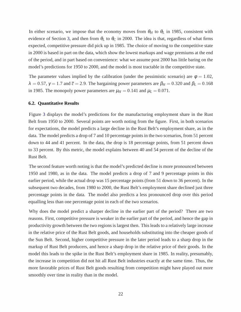
In either scenario, we impose that the economy moves fromθH to θL in 1985, consistent with

evidence of Section3, and then fromθL to θC in 2000. The idea is that, regardless of what firms

expected, competitive pressure did pick up in 1985. The choice of moving to the competitive state

in 2000 is based in part on the data, which show the lowest markups and wage premiums at the end

of the period, and in part based on convenience: what we assume post 2000 has little baring on the

model’s predictions for 1950 to 2000, and the model is most tractable in the competitive state.

The parameter values implied by the calibration (under the pessimistic scenario) areφ = 1.02,

λ = 0.57,γ = 1.7 andc= 2.9. The bargaining power parameters areβH = 0.320 andβL = 0.168

in 1985. The monopoly power parameters areµH = 0.141 andµL = 0.071.

6.2. Quantitative Results

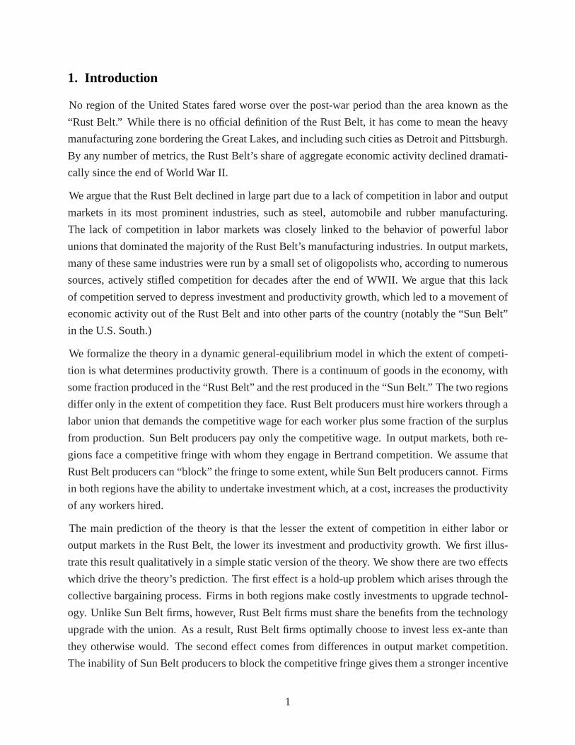
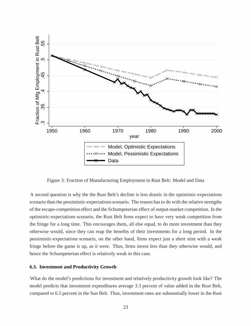
Figure3 displays the model’s predictions for the manufacturing employment share in the Rust

Belt from 1950 to 2000. Several points are worth noting from the figure. First, in both scenarios

for expectations, the model predicts a large decline in the Rust Belt’s employment share, as in the

data. The model predicts a drop of 7 and 10 percentage points in the two scenarios, from 51 percent

down to 44 and 41 percent. In the data, the drop is 18 percentage points, from 51 percent down

to 33 percent. By this metric, the model explains between 40 and 54 percent of the decline of the

Rust Belt.

The second feature worth noting is that the model’s predicted decline is more pronounced between

1950 and 1980, as in the data. The model predicts a drop of 7 and9 percentage points in this

earlier period, while the actual drop was 15 percentage points (from 51 down to 36 percent). In the

subsequent two decades, from 1980 to 2000, the Rust Belt’s employment share declined just three

percentage points in the data. The model also predicts a lesspronounced drop over this period

equalling less than one percentage point in each of the two scenarios.

Why does the model predict a sharper decline in the earlier part of the period? There are two

reasons. First, competitive pressure is weaker in the earlier part of the period, and hence the gap in

productivity growth between the two regions is largest then. This leads to a relatively large increase

in the relative price of the Rust Belt goods, and households substituting into the cheaper goods of

the Sun Belt. Second, higher competitive pressure in the later period leads to a sharp drop in the

markup of Rust Belt producers, and hence a sharp drop in the relative price of their goods. In the

model this leads to the spike in the Rust Belt’s employment share in 1985. In reality, presumably,

the increase in competition did not hit all Rust Belt industries exactly at the same time. Thus, the

more favorable prices of Rust Belt goods resulting from competition might have played out more

smoothly over time in reality than in the model.

22

.3.3

5.4

.45

.5.5

5F

ract

ion

of M

fg E

mpl

oym

ent i

n R

ust B

elt

1950 1960 1970 1980 1990 2000year

Model, Optimistic ExpectationsModel, Pessimistic ExpectationsData

Figure 3: Fraction of Manufacturing Employment in Rust Belt: Model and Data

A second question is why the the Rust Belt’s decline is less drastic in the optimistic-expectations

scenario than the pessimistic-expectations scenario. Thereason has to do with the relative strengths

of the escape-competition effect and the Schumpeterian effect of output-market competition. In the

optimistic-expectations scenario, the Rust Belt firms expect to have very weak competition from

the fringe for a long time. This encourages them, all else equal, to do more investment than they

otherwise would, since they can reap the benefits of their investments for a long period. In the

pessimistic-expectations scenario, on the other hand, firms expect just a short stint with a weak

fringe before the game is up, as it were. Thus, firms invest less than they otherwise would, and

hence the Schumpeterian effect is relatively weak in this case.

6.3. Investment and Productivity Growth

What do the model’s predictions for investment and relatively productivity growth look like? The

model predicts that investment expenditures average 3.3 percent of value added in the Rust Belt,

compared to 6.5 percent in the Sun Belt. Thus, investment rates are substantially lower in the Rust

23

Belt than in the remainder of the economy.

As a result, productivity growth rates are substantially lower in the Rust Belt. The model’s average

annualized productivity growth rate (in the pessimistic state) for Rust Belt producers is 1.4 percent;

in the Sun Belt this figure is 2.3 percent. Worth noting is thatpredicted productivity growth is

lowest in the early period in the Rust Belt, at 1.3 percent peryear from 1950 to 1980, and rises to

1.6 percent per year after 1980. In the Sun Belt, productivity growth is 2.4 percent per year before

1980 and falls slightly to 2.1 percent afterwards. Thus, thedifference in productivity growth rates

converged somewhat over the period. After 2000, in the competitive state, the model predicts that

productivity growth rates are both exactly two percent per year (as per the calibration.)

7. Supporting Evidence on Investment and Productivity Growth

In this section we present additional evidence on the model’s predictions for investment and pro-

ductivity growth. In particular, we consider evidence on R&D expenditures, TFP growth, and

technology adoption rates. While each has its limitations,taken together they support the model’s

prediction that investment and productivity growth were relatively low in Rust Belt industries for

most of the post-war period.

7.1. R&D Expenditures

The first piece of evidence we consider is on R&D expendituresby industry. Expenditures on

R&D provides a nice example of costly investments that are taken to improve productivity, as in

the model.

Evidence from the 1970s suggests that R&D expenditures werelower in key Rust Belt industries,

in particular steel, automobile and rubber manufacturing,than in other manufacturing industries.

According to a study by theU.S. Office of Technology Assessment(1980), the average manu-

facturing industry had R&D expenditures totaling 2.5 percent of total sales in the 1970s. The

highest rates were in communications equipment, aircraft and parts, and office and computing

equipment, with R&D representing 15.2 percent, 12.4 percent and 11.6 percent of total sales, re-

spectively. Auto manufacturing, rubber and plastics manufacturing, and “ferrous metals,” which

includes steelmaking, had R&D expenditures of just 2.1 percent, 1.2 percent and 0.4 percent of

total sales. These data are qualitatively consistent with the model’s prediction that investment rates

were lower in the Rust Belt than elsewhere in the United States.20

20Several sources explicitly link the lack of innovation backto a lack of competition. For example, about theU.S. steel producersAdams and Brock(1995) state that “their virtually unchallenged control over a continent-sizedmarket made them lethargic bureaucracies oblivious to technological change and innovation. Their insulation fromcompetition induced the development of a cost-plus mentality, which tolerated a constant escalation of prices and

24

Table 4: TFP Productivity Growth by Individual Rust Belt Industrie s

Annualized Growth Rate, %

1958-1980 1980-2000 1958-2000

Iron and Steel Foundries 0.0 0.5 0.2

Machinery, Misc −0.4 −0.1 −0.2

Motor Vehicles 1.0 0.2 0.6

Railroad Equipment 1.0 −0.3 0.3

Rubber Products −0.2 2.5 1.1

Steel Mills 0.4 0.9 0.7

Rust Belt Average 0.3 0.6 0.4

U.S. Economy 2.0 1.4 1.8

Note: Rust Belt Industries are defined as those industries whose employment shares in RustBelt MSAs are more than one standard deviation higher than the mean in both 1950 and2000. Source: Author’s calculations using NBER CES productivity database, U.S. censusdata from IPUMS, and the BLS.

7.2. Productivity Growth

Direct measures of productivity growth by region do not exist unfortunately. Nevertheless, we can

assess the model’s predictions for productivity growth in the Rust Belt by comparing estimates of

productivity growth in industries that were prominent in the Rust Belt region over the period 1950

to 2000 to productivity growth in the rest of the economy.

Concrete estimates of productivity growth by industry are available from the NBER CES database.21

By matching their industries (by SIC codes) to those available to us in our IPUMS census data (by

census industry codes), we are able to compute the fraction of all employment in each industry

that is located in the Rust Belt in each year. We define “Rust Belt industries” as all those industries

with employment shares in the Rust Belt greater than one standard deviation above the mean in

both 1950 and 2000. The industries that make the cut are Iron and Steel Foundries, Miscellaneous

Machinery, Motor Vehicles, Railroad Equipment, Rubber Products, and Steel Mills.

Table4 provides estimates of total-factor productivity (TFP) growth per year in these industries

over several time horizons. As a frame of reference, we compute TFP for the U.S. economy as

a whole as the Solow Residual from a Cobb-Douglas productionfunction with labor share two-

thirds and aggregate data from the BEA. The right-most column shows the entire period of data

wages and a neglect of production efficiency (page 93). ”21A detailed description of the data, and the data themselves,are available here: http://www.nber.org/nberces/.

25

availability, namely 1958-2000. TFP growth was lower in every Rust Belt industry than for the U.S.

economy as a whole. The highest growth was in Rubber Products, which grew at 1.1 percent per

year, while the lowest was in Machinery, which grew at -0.2 percent per year. The U.S. economy,

on the other hand, had far higher TFP growth of 1.8 percent peryear over this period.

The first and second two columns show TFP growth by industry inthe periods 1958-1980 and 1980

to 2000. We choose this breakdown based on the evidence of Section 3 that competition picked

up in the 1980s. The first two columns show that in four of the six industries – Iron and Steel

Foundries, Machinery, Rubber Products, and Steel Mills – productivity increased in the period

after 1980. This is consistent with the productivity pickupfound in the model in the latter part of

the period.

One limitation of these data is that what we define as Rust Beltindustries include a lot of economic

activity that does not take place in the Rust Belt. This is particularly true in the later period of the

sample, when the Rust Belt’s share of activity had fallen substantially. For the auto industry, we

address this concern (at least in part) by computing the rateof growth of automobiles produced

per worker for the Big Three auto makers, who had the majorityof their auto production in the

Rust Belt region, using company annual reports. We find that GM, Ford and Chrysler had average

annual productivity growth rates of 1.1 percent, 1.3 percent and 1.8 percent respectively.22 As

these growth rates are all lower than the economy-wide average of around 2 percent per year, they

suggest that Rust Belt automobile productivity growth was indeed lower than average.

For the steel industry,Collard-Wexler and De Loecker(2012) (Table 10) report TFP growth by

two broad types of producers: the vertically integrated mills, most of which were in the Rust Belt,

and the minimills, most of which were in the South. They find that for the vertically integrated

mills, TFP growth was very low from the period 1963 to 1982, and in fact negative for much of the

period. From 1982 to 2002 they report very robust TFP growth in the vertically integrated mills,

totaling 11 percent 1982 and 1987, and 16 percent between 1992 to 1997. This supports the claim

that Rust Belt steel productivity growth was relatively lowover the period before the 1980s, and

picked up only afterwards.

A second limitation of the productivity evidence of Table4 is that it compares Rust Belt industries

to other industries that may have differed in “potential productivity growth.” In other words, it

compares newer industries, such as computers, where there is a large scope for productivity growth,

than in more-established industries, such as steel and autos. To address this limitation, we compare

productivity growth in the U.S. steel and auto industries toforeign steel and auto industries. The

22The company reports are all publicly available from the companies themselves. The exact years used differ slightlyacross the three companies due to data availability. The data for GM, Ford and Chrysler begin in 1954, 1955 and 1950,respectively.

26

idea is that comparing the key Rust Belt industries to similar industries abroad, one can see how

the Rust Belt fared compared to other producers with similarscope for productivity growth.

For the auto industry,Fuss and Waverman(1991) compare the performance of the United States

industry to that of Japan. They calculate that between 1970 and 1980, TFP growth in the Japanese

auto manufacturing industry averaged 4.3 percent per year.In the U.S. auto industry, in contrast,

TFP growth averaged just 1.6 percent.23 For the steel industry,Lieberman and Johnson(1999)

(Figure 8) compute that TFP in the U.S. vertically integrated mills was roughly constant from

1950 to 1980. Over the same period, TFP in the Japanese steel industry roughlydoubled.Thus,

in both the auto and steel industry, evidence suggests that the Rust Belt producers experienced

productivity growth substantially below that of the foreign producers in their same industries.

7.3. Technology Adoption

Another proxy for productivity-enhancing investment activity is the rate of adoption of key productivity-

enhancing technologies. For the U.S. steel industry before1980, the majority of which was in the

Rust Belt, there is a strong consensus that adoption rates ofthe most important technologies lagged

far behind where they could have been (Adams and Brock, 1995; Adams and Dirlam, 1966; Lynn,

1981; Oster, 1982; Tiffany, 1988; Warren, 2001). The two most important new technologies of

the decades following the end of WWII were the basic oxygen furnace (BOF) and the continuous

casting method. Figure7 shows adoption rates of continuous casting methods in the United States,

Japan and several other leaders in steel production. Two things are worth noting from this figure.

First, the United States was a laggard, with only 15 percent of its capacity produced using contin-

uous casting methods, compared to a high of 51 percent in Japan, by 1978. Second, this was the

period where large integrated steel mills of the Rust Belt dominated production. Putting these two

observations together implies that the Rust Belt lagged farbehind in the adoption of one important

technology over the period.24

There is also agreement that the U.S. steel industry had ample opportunities to adopt the new

technologies and chose not to do so. For exampleLynn (1981) states that “the Americans appear

to have had more opportunities to adopt the BOF than the Japanese when the technology was

relatively new. The U.S. steelmakers, however, did not exploit their opportunities as frequently as

the Japanese.” Regarding the potential for the U.S. Steel Corporation to adopt the BOF,Warren

23Norsworthy and Malmquist(1983) find slightly lower numbers for an earlier period, but stillfind lower TFPgrowth for the U.S. auto industry than for the Japanese auto industry.

24In the 1980s and afterward, the U.S. steel industry made large investments in a new technology, the minimill,which used an electric arc furnace to turn used steel products into raw steel for re-use. Virtually all of these adoptionswere made outside of the Rust Belt region, and in the U.S. South in particular. SeeCollard-Wexler and De Loecker(2012) and the references therein.

27

(2001) describes the 1950s and 1960s as “a period of unique but lostopportunity for American

producers to get established early in the new technology.”25

The view that technology adoption in the U.S. steel industrywas inefficiently low is in fact con-

firmed by the producers themselves. In their 1980 annual report, the American Iron and Steel

Institute (representing the vertically integrated U.S. producers) admit that:

Inadequate capital formation in any industry produces meager gains in productiv-

ity, upward pressure on prices, sluggish job creation, and faltering economic growth.

These effects have been magnified in the steel industry. Inadequate capital formation ...

has prevented adequate replacement and modernization of steelmaking facilities, thus

hobbling the industry’s productivity and efficiency (American Iron and Steel Institute,

1980).

Similar evidence can be found for the rubber and automobile manufacturing industries. In rubber

manufacturing,Rajan, Volpin, and Zingales(2000) andFrench(1991) argue that U.S. tire man-

ufacturers missed out on the single most important innovation of the postwar period, which was

the radial tire, adopting only when it was too late (in the mid1980s). The big innovator of the

radial tire was (the French firm) Michelin (in the 1950s and 1960s). According toFrench(1991),

most of the U.S. rubber tire producers hadn’t adopted radials even by the 1970s, even as Michelin

drastically increased its U.S. market share.

The sluggish rate of technology adoption by the auto industry seems to be widely acknowledged

by industry historians and insiders, such asAdams and Brock(1995), Ingrassia(2011) andVlasic

(2011). As one example,Halberstam(1986) writes

Since competition within the the [automobile manufacturing] industry was mild,

there was no incentive to innovate; to the finance people, innovation not only was

expensive but seemed unnecessary... From 1949, when the automatic transmission

was introduced, to the late seventies, the cars remained remarkably the same. What

innovation there was came almost reluctantly (p. 244).

To summarize the results of this section, investment and productivity growth seemed to be lower

among Rust Belt industries than other U.S. industries, and lower than they could have been given

25As just one example,Ankl and Sommer(1996) report an engineer at the U.S. Steel Company visited the AustrianLinz BOF plant in 1954 and brought back a favorable report on the prospects of the BOF. Management at U.S. Steelvetoed this line of research and reprimanded the engineer for making an unauthorized visit to the Austrian firm (pp161-162.)

28

available investment opportunities, particularly beforethe 1980s. This supports the model’s predic-

tions that Rust Belt investment and productivity growth rates were low, and particularly so before

the 1980s when competition was at its lowest.

8. Supporting Evidence from Cross-Section of MetropolitanAreas

In this section we provide some additional evidence that supports the role of limited competition

in the Rust Belt’s decline. Specifically, we look beneath thesurface of the regional aggregates

focused on until now, and consider the cross-section of Metropolitan Statistical Areas (MSAs)

within the United States. What we show is that MSAs that had the lowest employment growth

over the period 1950 to 2000 tended to be those that paid workers the highest wage premiums in

1950. Our results in this section corroborate the earlier results ofBorjas and Ramey(2000), who

document thatindustriespaying the highest wage premiums in 1959 had the lowest employment

growth through 1989. As many of the high-wage industries in their study (e.g. autos and steel)

were concentrated in the high-wage MSAs of our study (e.g Detroit and Pittsburgh), we conclude

that both sets of evidence are consistent with the basic prediction of the model.

The data we use for this analysis is the decennial census micro data available from IPUMS. The

unit of geography is, as mentioned above, the MSA, which corresponds roughly to a city plus its

surrounding suburbs. We report MSA-level statistics for all MSAs in the country that are above

a certain size threshold (determined by the Census Bureau),usually around 100,000 people. The

place of residence is excluded for confidentiality reasons in smaller MSAs or rural areas. We also

focus attention to 3-digit MSAs as defined by IPUMS, as these have changed definition relatively

infrequently over time (unlike the 4-digit MSAs.)

We consider all workers who report being primarily wage earners, as opposed to the self-employed,

and only those employed in the private sector. The reason forthese restrictions are to limit possible

biases in our measurement of wage premiums, as well as to keepour sample as standard as possible.

We note that our results carry over to alternative sample restrictions, such as only men, only full-

time workers, only household heads, and combinations thereof.

We construct our measures of wage premiums as follows. As in many standard macroeconomic

models, we assume that under competition, the workers’ wageshould be proportional to their

human capital. Following the tradition of Mincer, we assumethat a worker’s human capital is a

function their schooling and potential work experience. Webuild on these assumptions by letting a

worker’s wage depend on where they live, with some regions offering a larger payment per unit of

human capital than others. In particular, we assume that thelog hourly wage of workeri in region

29

m is

logwi,m = α ·SCHOOLi,m+4

∑j=1

β j ·EXPERji,m+

M

∑m=1

Dm ·πm+ εi,m (23)

whereSCHOOLi,m andEXPERi,m represent years of schooling and potential experience,Dm is a

dummy for residing in regionm, andεi,m is an error term. The coefficientsα andβ1 throughβ4

capture the returns to schooling and experience while theπm terms capture the “premium” that a

worker earns for living in regionmcontrolling for schooling and experience.

We estimate (23) using the IPUMS micro data (from 1950), and take theπm terms as our measure

of wage premiums by MSA. We emphasize that these measures arebest thought of as suggestive

due to the crude way in which they are calculated. One limitation for example is that other poten-

tially important MSA-level characteristics are omitted from the regression, such as cost-of-living

indices. Another limitation is that schooling and potential experience themselves are imperfect

proxies for human capital. Nevertheless, we argue that these wage premium measures are still

useful in describing and understanding regional differences in economic performance over the

post-war period.

Figure4 shows the wage premium in 1950 (normalized to 0) plotted against the annualized growth

in employment from 1950 to 2000. Rust Belt MSAs are displayedin black, while the rest are grey.

As can be seen in the figure, there is a negative correlation between the two variables, with regions

with the highest premiums in 1950 tending to have the worst subsequent employment growth. The

correlation coefficient is -0.44, and is significant at well below the 1-percent level.

Which are the regions on either end of the spectrum? Among theMSAs with high wage premi-

ums are South Bend, IN (SOB), Detroit, MI (DET), Jackson, MI (JCS), Chicago-Gary-Lake, IL

(CHI), Pittsburgh, PA (PIT), Youngstown-Warren, OH (WAR),and Flint, MI (FLI). Each of these

MSAs was home in 1950 to a major manufacturing center in the automobile or steel industries.26

Among those with low wage premiums are Orlando, FL (ORL), Austin, TX (AUS), Phoenix,

AZ (PHX), Raleigh-Durham, NC (RAL) and Greensboro-WinstonSalem-High Point, NC (GRB).

These MSAs have all been referred to as being part of the “Sun Belt” (by Blanchard and Katz

(1992), among others).

One potential alternative theory of the wage premiums in theRust Belt is that workers there tended

to be of higher-than-average ability. This could be the case, say, if talented workers in the 1950s

tended to be attracted disproportionately to the Rust Belt regions because labor markets there were

strong at the time. According to this theory, the interpretation of the above-average wages as

26See e.g.Vlasic (2011) or Ingrassia(2011) on auto manufacturing, andTiffany (1988) or Crandall(1981) on steel.South Bend, Detroit, Jackson and Flint were major auto producers; Pittsburgh, Youngstown-Warren and Chicago-Gary-Lake were steelmaking centers.

30

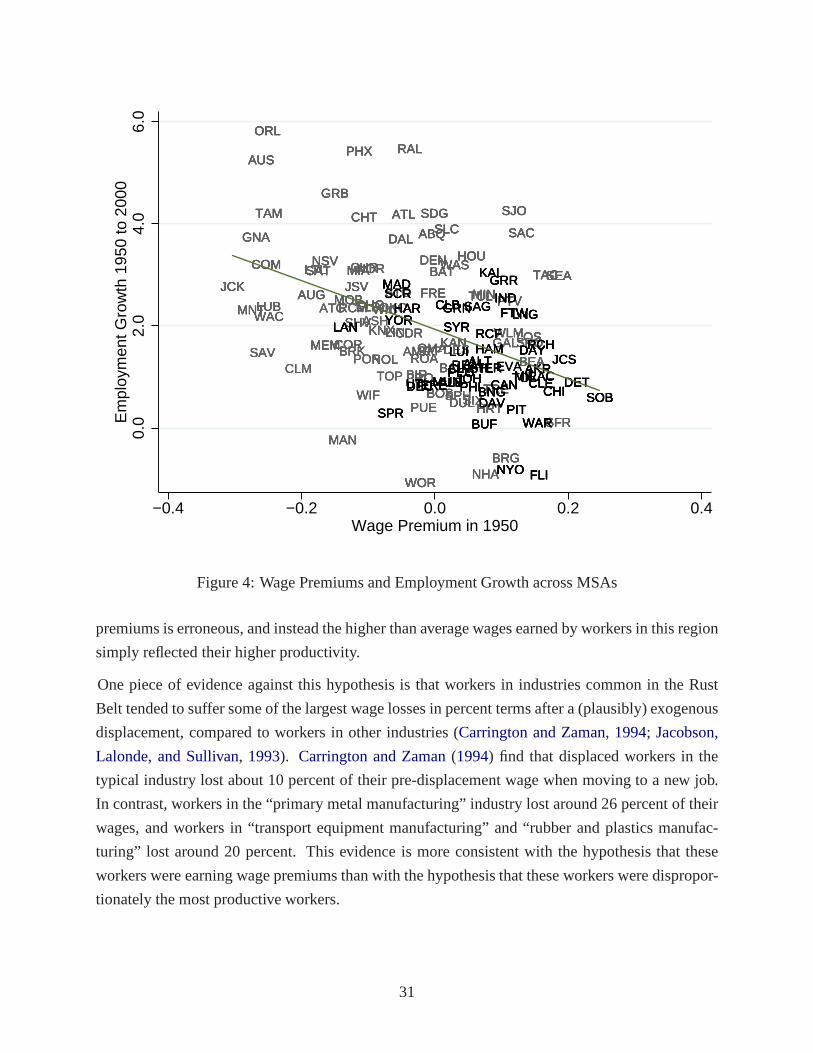
ABQABQABQABQABQ

AMRAMRAMRAMR

ASHASHASH

ATLATLATLATLATL

ATCATCATCATCAUGAUGAUGAUGAUG

AUSAUSAUSAUSAUS

BALBALBALBALBAL

BATBATBATBATBAT

BEABEABEABEABEA

BNGBIRBIRBIRBIRBIR

BOSBOSBOSBOSBOS

BRGBRGBRGBRGBRG

BRKBRKBRKBRKCDRCDRCDRCDR

CHRCHRCHRCHRCHR

CHTCHTCHTCHTCHT

CHOCHOCHOCHOCHO

COMCOMCOMCOMCOM

CLMCLMCLM

CORCORCORCORCOR

DALDALDALDALDAL

DAV

DENDENDENDENDEN

DESDESDESDESDES

DULDULDULDULDUL

ELPELPELPELPELPFREFREFREFREFRE

GALGALGALGAL

GRBGRBGRBGRBGRB

GNAGNAGNAGNAGNA

HRTHRTHRTHRTHRT

HOUHOUHOUHOUHOU

JCKJCKJCKJCKJCK JSVJSVJSVJSVJSV

KANKANKANKANKANKNXKNXKNXKNXKNXLINLINLINLIN

LTLLTLLTLLTLLTL

LOSLOSLOSLOSLOSLUILUI

LUBLUBLUBLUB

MANMANMANMAN

MEMMEMMEMMEMMEM

MIAMIAMIAMIAMIA

MINMINMINMINMINMOBMOBMOBMOBMOBMNTMNTMNTMNT

NSVNSVNSVNSVNSV

NHANHANHANHA

NOLNOLNOLNOLNOL

NORNORNORNOR

OKCOKCOKCOKCOKC

OMAOMAOMAOMAOMA

ORLORLORLORLORL

PHXPHXPHXPHXPHX

PORPORPOR

PTVPTVPTVPTVPTV

PROPROPROPROPRO

PUEPUEPUEPUE

RALRALRALRAL

RCMRCMRCMRCMRCM

ROAROAROAROA

SACSACSACSACSACSLCSLCSLCSLCSLC

SATSATSATSATSAT

SDGSDGSDGSDGSDG

SFRSFRSFRSFRSFR

SJOSJOSJOSJOSJO

SAVSAVSAVSAV

SEASEASEASEASEA

SHVSHVSHVSHVSHV

SIXSIXSIX

SXFSXFSXFSPOSPOSPOSPOSPO

SPHSPHSPHSPHSPH

STOSTOSTOSTOSTOTACTACTACTACTAC

TAMTAMTAMTAMTAM

TOLTOPTOPTOPTRETRETRETRETRE

TULTULTULTULTUL

WACWACWACWAC

WASWASWASWASWAS

WICWICWICWICWIC

WIFWIFWIFWIF

WLMWLMWLMWLMWLM

WORWORWORWORWOR

AKRAKRAKRAKRAKRALBALBALBALBALB

ALLALLALLALLALLALTALTALTALT

BNGBNGBNGBNG

BUFBUFBUFBUFBUF

CANCANCANCANCAN CHICHICHICHICHI

CINCINCINCINCINCLECLECLECLECLE

CLBCLBCLBCLBCLB

DAVDAVDAVDAV

DAYDAYDAYDAYDAY

DECDECDECDEC DETDETDETDETDETEREEREEREEREERE

EVAEVAEVA

FLIFLIFLIFLIFLI

FTWFTWFTWFTWFTW

GRRGRRGRRGRRGRR

GRNGRNGRNGRN

HAMHAMHAMHAM

HARHARHARHARHARINDINDINDINDIND

JCSJCSJCSJCS

JOHJOHJOHJOHJOH

KALKALKALKAL

LANLANLANLANLANLNGLNGLNGLNGLNG

LUILUILUI

MADMADMADMADMAD

MILMILMILMILMILMUNMUNMUNMUN

NYONYONYONYONYO

PEOPEOPEOPEOPEOPHIPHIPHIPHIPHI

PITPITPITPITPIT

RACRACRACRACREAREAREAREAREA

RCHRCHRCHRCHRCHRCFRCFRCFRCFRCF

SAGSAGSAGSAG

STLSTLSTLSTLSTL

SCRSCRSCRSCR

SOBSOBSOBSOBSOBSPRSPRSPRSPR

SYRSYRSYRSYRSYR

TERTERTERTERTOLTOLTOLTOLUTIUTIUTIUTIUTI

YORYORYORYORYOR

WARWARWARWARWAR

0.0

2.0

4.0

6.0

Em

ploy

men

t Gro

wth

195

0 to

200

0

−0.4 −0.2 0.0 0.2 0.4Wage Premium in 1950

Figure 4: Wage Premiums and Employment Growth across MSAs

premiums is erroneous, and instead the higher than average wages earned by workers in this region

simply reflected their higher productivity.

One piece of evidence against this hypothesis is that workers in industries common in the Rust

Belt tended to suffer some of the largest wage losses in percent terms after a (plausibly) exogenous

displacement, compared to workers in other industries (Carrington and Zaman, 1994; Jacobson,

Lalonde, and Sullivan, 1993). Carrington and Zaman(1994) find that displaced workers in the

typical industry lost about 10 percent of their pre-displacement wage when moving to a new job.

In contrast, workers in the “primary metal manufacturing” industry lost around 26 percent of their

wages, and workers in “transport equipment manufacturing”and “rubber and plastics manufac-

turing” lost around 20 percent. This evidence is more consistent with the hypothesis that these

workers were earning wage premiums than with the hypothesisthat these workers were dispropor-

tionately the most productive workers.

31

9. Conclusion

While the U.S. economy as a whole experienced robust economic growth over the postwar period,

there was substantial variation in the economic performance of regions within the country. No

region fared worse than the Rust Belt, the heavy manufacturing zone bordering the Great Lakes.

The Rust Belt’s share of employment and value added fell drastically over this period, both overall

and within the manufacturing sector.

Our theory is that a lack of competition was behind the Rust Belt’s poor economic performance.

We formalize our theory in a dynamic general equilibrium model in which productivity growth is

driven by the strength of competition in labor and output markets. Non-competitive labor mar-

kets lead to a hold-up problem between workers and firms, which discourage firms from investing.

Non-competitive output markets reduce the firm’s incentiveto invest in order to escape the compe-

tition. A plausibly calibrated version of the model predicts roughly one-half of the decline found in

the data. The model also predicts that the Rust Belt lagged behind in investment in new technolo-

gies and productivity growth. These predictions are borne out in several types of evidence from

prominent Rust Belt industries.

32

References

ACEMOGLU, D., AND U. AKCIGIT (2011): “Intellectual Property Rights Policy, Competition and

Innovation,”Journal of the European Economic Association, 10(1), 1–42.

ACIKGOZ, O. T., AND B. KAYMAK (2012): “The Rising Skill Premium and Deunionization in

the United States,” Unpublished Manuscript, Universite deMontreal.

ADAMS, W., AND J. BROCK (eds.) (1995):The Structure of American Industry. Prentice-Hall,

Inc.

ADAMS, W., AND J. B. DIRLAM (1966): “Big Steel, Invention, and Innovation,”Quarterly Jour-

nal of Economics, 80(2), 167–189.

AGHION, P., N. BLOOM, R. BLUNDELL , R. GRIFFITH, AND P. HOWITT (2005): “Competition

and Innovation: An Inverted U Relationship,”Quarterly Journal of Economics.

AMERICAN IRON AND STEEL INSTITUTE (1980): “Steel at the Crossroads: The American Steel

Industry in the 1980s,” .

ANKL , R., AND E. SOMMER (1996): The Role of Management in the Decline of the American

Steel Industry.

BERNARD, A. B., J. EATON, AND J. B. JENSEN (2003): “Plants and Productivity in International

Trade,”American Economic Review, 93(4), 1268–1290.

BERNDT, E. R., A. F. FRIEDLAENDER, AND J. S.-E. W. CHIANG (1990): “Interdependent Pric-

ing and Markup Behavior: An Empirical Analysis of GM, Ford and Chrysler,” NBER Working

Paper No. 3396.

BLANCHARD , O., AND L. KATZ (1992): “Regional Evolutions,”Brookings Papers on Economic

Activity, 1992(1).

BLANCHFLOWER, D. G., AND A. BRYSON (2004):The Union Wage Premium in the US and the

UK. Centre for Economic Performance.

BLOOM, N., M. DRACA, AND J. VAN REENAN (2011): “Trade Induced Technical Change? The

Impact of Chinese Imports on Innovation, IT and Productivity,” NBER Working Paper 16717.

BORJAS, G. J.,AND V. A. RAMEY (1995): “Wage Inequality and Trade,”Quarterly Journal of

Economics, 110, 1075–1110.

33

(2000): “Market Responses to Interinustry Wage Differentials,” NBER Working Paper

7799.

BRIDGMAN , B. (2011): “Competition, Work Rules and Productivity,” Unpublished Manuscript,

Bureau of Economic Analysis.

BRODA, C., AND D. WEINSTEIN (2006): “Globalization and the Gains from Variety,”Quarterly

Journal of Economics, 121(2).

CARRINGTON, W., AND A. ZAMAN (1994): “Interindustry Variation in the Costs of Job Displace-

ment,”Journal of Labor Economics, 12(2), 243–275.

COLE, H. L., AND L. E. OHANIAN (2004): “New Deal Policies and the Persistence of the Great

Depression: A General Equilibrium Analysis,”Journal of Political Economy, 112(4), 779–816.

COLLARD-WEXLER, A., AND J. DE LOECKER (2012): “Reallocation and Technology: Reallo-

cation and Technology: Evidence from the U.S. Steel Industry,” Unpublished Manuscript, New

York University.

CRANDALL , R. W. (1981): The U.S. Steel Industry in Recurrent Crisis. Brookings Institution

Press.

DINLERSOZ, E., AND J. GREENWOOD(2012): “The Rise and Fall of Unions in the U.S.,” Unpub-

lished Manuscript, University of Pennsylvania.

DUNNE, T., S. KLIMEK , AND J. A. SCHMITZ (2010): “Competition and Productivity: Evidence

from the Post WWII U.S. Cement Industry,” Unpublished Manuscript, U.S. Census Bureau.

FEYRER, J., B. SACERDOTE, AND A. D. STERN (2007): “Did the Rust Belt Become Shiny? A

Study of Cities and Counties That Lost Steel and Auto Jobs in the 1980s,”Brookings-Wharton

Papers on Urban Affairs, pp. 41–102.

FRENCH, M. J. (1991):The U.S. Tire Industry. Twayne Publishers, Boston.

FUSS, M., AND L. WAVERMAN (1991): “Productivity Growth in the Motor Vehicle Industry,

1970-1984: A Comparison of Canada, Japan, and the United States,” inProductivity Growth in

Japan and the United States, ed. by C. Hulten, pp. 85–108. University of Chicago Press.

GLAESER, E. L., AND G. A. PONZETTO (2007): “Did the Death of Distance Hurt Detroit and

Help New York?,” Unpublished Manuscript, Harvard University.

GOLDFIELD, M. (1987):The Decline of Organized Labor in the United States. The University of

Chicago Press, Chicago.

34

HALBERSTAM, D. (1986):The Reckoning. William Morrow and Company, Inc.

HERRENDORF, B., AND A. TEIXEIRA (2011): “Barriers to Entry and Development,”International

Economic Review, 52(2), 573–602.

HIRSCH, B. T., AND D. A. MACPHERSON(2003): “Union Membership and Coverage Database

from the Current Population Survey: Note,”Industrial and Labor Relations Review, 56(2), 349–

54.

HOERR, J. (1988):And the Wolf Finally Came. University of Pittsburgh Press.

HOLMES, T. J. (1998): “The Effect of State Policies on the Location of Manufacturing: Evidence

from State Borders,”Journal of Political Economy, 106(4), 667–705.

HOLMES, T. J., AND J. A. SCHMITZ (2010): “Competition and Productivity: A Review of Evi-

dence,”Annual Review of Economics, 2, 619–642.

HUDSON, R., AND D. SADLER (1989): The International Steel Industry: Restructuring, State

Policies, and Localities. Routledge.

INGRASSIA, P. (2011):Crash Course. Random House, New York.

JACOBSON, L. S., R. J. LALONDE, AND D. G. SULLIVAN (1993): “Earnings Losses of Displaced

Workers,”American Economic Review, 83(4), 685–709.

KAHN , M. E. (1999): “The Silver Lining of the Rust Belt Manufacturing Decline,” Journal of

Urban Economics, 46, 360–376.

KLIER, T. H. (2009): “From Tail Fins to Hybrids: How Detroit Lost its Dominance of the U.S.

Auto Market,”Economic Perspectives, 30(2), 2–13.

L IEBERMAN, M. B., AND D. R. JOHNSON (1999): “Comparative Productivity of Japanese and

U.S. Steel Producers, 1958-1993,”Japan and the World Economy, 11, 1–27.

LYNN , L. (1981): “New Data on the Diffusion of the Basic Oxygen Furnace in the U.S. and Japan,”

Journal of Industrial Economics, 30(123-135).

MCGRATTAN , E. R., AND E. C. PRESCOTT (2010): “Technology Capital and the U.S. Current

Account,”American Economic Review, 100(4), 1493–1522.

NGAI , R. L., AND C. A. PISSARIDES (2007): “Structural Change in a Multisector Model of

Growth,” American Economic Review, 97(1).

35

NORSWORTHY, J., AND D. H. MALMQUIST (1983): “Input Measurement and Productivity

Growth in Japnese and U.S. Manufacturing,”American Economic Review, 73(5), 947–967.

OSTER, S. (1982): “The Diffusion of Innovation among Steel Firms:The Basic Oxygen Furnace,”

Bell Journal of Economics, 13(1), 45–56.

PARENTE, S. L., AND E. C. PRESCOTT(1999): “Monopoly Rights: A Barrier to Riches,”Ameri-

can Economic Review, 89(5), 1216–1233.

PAVCNIK , N. (2002): “Trade Liberalization, Exit and Productivity Improvement: Evidence from

Chilean Plants,”Review of Economic Studies, 69(1), 245–276.

RAJAN, R. G., P. VOLPIN, AND L. Z INGALES (2000): “The Eclipse of the U.S. Tire Industry,” in

Mergers and Productivity, ed. by S. N. Kaplan, pp. 51–92. University of Chicago Press.

RUGGLES, S. J., T. ALEXANDER, K. GENADEK, R. GOEKEN, M. SCHROEDER, AND M. SOBEK

(2010): “Integrated Public Use Microdata Series: Version 5.0,” [Machine-readable database].

Minneapolis: University of Minnesota.

SCHMITZ , J. A. (2005): “What Determines Productivity? Lessons fromthe Dramatic Recovery

of the U.S. and Canadian Iron Ore Industries Following TheirEarly 1980s Crisis,”Journal of

Political Economy, 113(3), 582–625.

(2012): “New and Larger Costs of Monopoly and Tariffs,” Federal Reserve Bank of

Minneapolis Staff Report 468.

SYVERSON, C. (2011): “What Determines Productivity?,”Journal of Economic Literature, 49(2),

326–365.

TASCHEREAU-DUMOUCHEL, M. (2012): “The Union Threat,” Unpublished Manuscript, The

Wharton School of the University of Pennsylvania.

TIFFANY, P. A. (1988):The Decline of American Steel. Oxford University Press.

U.S. OFFICE OF TECHNOLOGY ASSESSMENT(1980): “Technology and Steel Industry Com-

petiveness,” U.S. Government Printing Office.

VAN REENEN, J. (1996): “The Creation and Capture of Rents: Wages and Innovation in a Panel

of U.K. Companies,”Quarterly Journal of Economics, 111(1), 195–226.

VLASIC, B. (2011):Once Upon a Car: The Fall and Resurrection of America’s Big Three Auto

Makers–GM, Ford, and Chrysler. Harper Collins.

36

WARREN, K. (2001):Big Steel: The First Century of the United States Steel Company, 1901-2001.

University of Pittsburgh Press.

YOON, C. (2012): “The Decline of the Rust Belt: A Dynamic Spatial Equilibrium Analysis,”

Unpublished Manuscript, University of Pennsylvania.

37

5010

015

020

0M

anuf

actu

ring

Em

ploy

men

t (19

50=

100)

1950 1960 1970 1980 1990 2000

Rust Belt United States ex. Rust Belt

Figure 5: Manufacturing Employment in Rust Belt and Rest of United States

38

10

15

20

25

30

35

Perc

ent

1920 1940 1960 1980 2000 2020

year

United States Rust Belt

United States excl. Rust Belt

Figure 6: Unionization Rate in the United States and by Region

39

010

20

30

40

50

Percent

1968 1970 1972 1974 1976 1978

year

US Japan

Germany Italy

France

Figure 7: Fraction of Steel Made Using Continuous Casting Process

40