THE SEARCH OF ECONOMIC STATE VARIABLES FOR … · simposium nasional akuntansi 9 padang padang, 23-26 agustus 2006 1 the search of an economic state variable

SIMPOSIUM NASIONAL AKUNTANSI 9 PADANG

Padang, 23-26 Agustus 2006 1

THE SEARCH OF AN ECONOMIC STATE VARIABLE FOR INTER-TEMPORAL ASSET PRICING:

EVIDENCE FROM JAKARTA STOCK EXCHANGE

ERNI EKAWATI1

Universitas Kristen Duta Wacana

ABSTRACT

Three-factor capital asset pricing model (CAPM)-beta, size, and book-to-market equity appears to dominate most other variables in the empirical explanation of cross-sectional returns. This study attempts to find a link between the prominent three-factor CAPM and the dynamic feature of inter-temporal CAPM by searching a simple ex-ante economic state variable. Using data from Jakarta Stock Exchange, this study finds that the three-factor CAPM holds in the full sample. After separating the samples into stable and unstable economic conditions, the result indicates that the risk premiums associated with the three-factor CAPM do vary, but the magnitudes of the variation cannot be observed due to some statistical problems. However, an ex-ante economic state variable, growth of change in money supply, proposed in this study fails to capture the time varying risk premiums attached in the three-factor CAPM.

1 Fakultas Ekonomi UKDW, Jl. Dr. Wahidin 5-21 Jogjakarta 55224.Telpon: (0274) 563929 pswt. 221. HP: 0811255921

K-INT 12



I. INTRODUCTION

The relationship between risk and return has been the focus of recent capital market

research. Numerous papers have derived various version of the capital asset pricing

model (CAPM), ranging from single-factor CAPM (Sharpe-Lintner and Black

versions), conditional CAPM (Engle, 1982 and Bollerslev, 1986), Arbitrage Pricing

Theory (Ross, 1976, Huberman, 1982, Chamberlain and Rothschild, 1983, Lehman and

Modest, 1988), three-factor CAPM (Fama and French, 1992, 1995; Chan, Jagedeesh,

and Lakonishok, 1995), intertemporal CAPM (Merton, 1973, and Breeden’s, 1979), to

international CAPM (Solnik, 1974, Korajczyk and Viallet, 1989). The role of beta in

explaining the cross-sectional variation in stock returns are well documented. In fact,

beta has a rich theoretical foundation but lacks empirical support. Two variables found

to be prominent in explaining the cross-sectional variation of return are size, as

measured by market value of equity, and book-to-market equity. These two variables

combined with beta (three-factor CAPM) appear to dominate most other variables in the

empirical explanation of cross-sectional returns.

The purpose of this study is to find a link between the prominent three-factor

CAPM and the dynamic feature of inter-temporal CAPM. In a dynamic economy, it is

often believed that if an investor anticipate information shifts, he will adjust his

portfolio to hedge these shifts. To capture the dynamic hedging effect, Merton (1973)

develops a continuous-time asset pricing model which explicitly takes into account

hedging demand. In contrast to the APT framework (employing undefined numbers of

state variables), there are only two factors which are theoretically derived from

Merton’s model (1973): a market factor and a hedging factor. However, an empirical

investigation is not easy to implement for the continuous-time model.

This study is intended to determine whether the premiums attached to the three-

factor CAPM vary in a predictable manner as the concern of investors shifts due to the

availability of anticipated information. Like Merton’s (1973), Breeden’s (1979), and

Jensen and Mercer (2002) efforts, approach of this study is to search the

macroeconomic state variables for inter-temporal asset pricing. Using three-factor

CAPM and employing the stock return of companies listed in Jakarta Stock Exchange

from the years of 1991 to 2000, this study will firstly, test the three-factor CAPM

K-INT 12



whether the premiums attached to the factors vary overtime across different economic

conditions. The observable different ex-post economic conditions are used. The sample

of the Indonesian data from the periods of 1991 to 2000 make the separation of the

different economic conditions possible. Indonesia experienced a stable economic

condition from the periods of 1991 to 1997, while the rest is an unstable condition,

following the economic crisis in 1998. If an inter-temporal variation occurs, it means

that the attached premiums vary across different observable economic conditions.

Finding an anticipated economic state variable is required. Secondly, find a common

anticipated economic state variable to link business conditions and market participants’

expectations about future market conditions. The state variable proposed is growth of

change in money supply (M2). Positive (negative) growth of change in money supply

represents an expansive (a restrictive) economic condition.

The perception that lack of information about the price behavior and

characteristics of emerging equity market hinders the foreign investments, has

motivated this study to find an economic state variable that can explain the time varying

expected behavior of asset pricing. In general, the finding of an anticipated state

economic variable can expectantly provide an important piece of contributions to the

puzzle surrounding the search for economic state variables in asset pricing model.

Specifically, this study will provide empirical evidence on a relevant state variable of

asset pricing from Jakarta Stock Exchange as one of the potential emerging markets in

the world.

II. THEORETICAL BACKGROUND

For the past three decades mean variance capital asset pricing model of Sharpe-Lintner

and Black have served as the corner stone of financial theory. The model has a long

history of theoretical and empirical investigation. The followings present a theoretical

review of the model and its developments.

A. Single Factor CAPM

The single factor CAPM of Sharpe-Lintner model is the extension of one period mean-

variance portfolio models of Markowitz (1959) and Tobin (1958), which in turn are

built on the expected utility model of Von Neumann and Morgenstern (1953). The

K-INT 12



Sharpe-Lintner asset pricing model then uses the characteristics of the consumer wealth

allocation decision to derive the equilibrium relationship between risk and expected

return for assets and portfolios. Making a number of assumptions, Sharpe-Lintner

extends Markowitz’s mean variance framework to develop a relation for expected

return, which can be written as:

))((()( fmifi RRERRE −+= β

where is expected return on ith security, is risk-free rate, is expected

return of market portfolio, and

)( iRE fR )( mRE

iβ is the measure of risk or definition of market

sensitivity parameter defined as cov(Ri, Rm)/var(Rm).

Intuitively, in a rational and competitive market investors diversify all

unsystematic risk away and thus price assets according to a single factor, namely,

systematic or non-diversifiable risk. The single factor CAPM, which describes stock

return solely on β measure, is based on the assumption that all market participants share

identical subjective expectations of mean and variance of return distribution, called

constant expected returns. Thus, a single-factor CAPM is classified as static asset

pricing model.

B. Inter-temporal CAPM

Unlike constant expected return assumed in single-factor CAPM, it has been observed

that return distribution varies over time (Engle, 1982 and Bollerslev, 1986). In other

words, the stock return distribution is time variant in nature and hence, the subjective

expectations of moment differ from one period to another. This implies that the

investors expectations of moments behave like random variables rather than constant as

assumed in the single-factor CAPM.

Since Merton (1973) finding of inter-temporal CAPM, the single-period CAPM

has been empirically challenged. There are ample evidence on time varying risk

premium, such as Keim and Stambaugh (1986), Fama and French (1988), French,

Schwert, and Stambaugh (1987). They claim that the concept of time-varying risk

premium cannot be properly explored within a static model such as single-factor CAPM

K-INT 12



or even static Arbitrage Pricing Theory (APT). In contrast to the APT framework

(employing undefined numbers of state variables), there are two factors which are

theoretically derived from Merton’s inter-temporal CAPM (1973): a market factor and a

hedging factor. The state variables are used to identify a hedging factor. In a dynamic

economy, if an investor anticipates information shifts, he will adjust his portfolio to

hedge these shifts.

Nielson and Vassalou (2001) specified two relevant variables for inter-temporal

CAPM, namely, instantaneous Sharpe ratio represented a market factor and real interest

rate represented a hedging factor. They demonstrated that investors hedge only against

stochastic changes in the slope and the intercept of the instantaneous capital market line,

which implied that only variables that forecast the real interest rate and the Sharpe ratio

will be priced.

C. Three-Factor CAPM

Recent researches show that single-factor specification of asset pricing model is

inappropriate (Fama and French, 1992, 1995, 1996, Jagannathan and Wang, 1996).

Fama’s and French’s three-factor CAPM uses beta, market equity, and book-to-market

equity as variables determining factor loadings in asset pricing. The three-factor model

is stated as follows:

)()())((()( HMLEhSMBEsRREbRRE iifmifi ++−=−

where , E(SMB)fi RRE −)( 2, and E(HML)3 are expected risk premiums. Fama and

French suggest that inter-temporal CAPM is one possible reason for the risk premiums

that they find to be associated with loadings on SMB and HML hedge portfolios. Fama

and French (1995) argue that the premiums are consistent with a multi-factor version of

Merton’s (1973) inter-temporal CAPM in which market equity and book-to market

equity proxy for sensitivity to risk factors in returns.

Liew and Vassalou (2000) report that annual returns on the SMB and HML

portfolios predict GDP growth in several countries. Vassalou (2002) shows that a

2 SMB is the difference between small market equity return and big market equity return portfolios. 3 HML is the difference between high BE/ME return and low BE/ME return portfolios.

K-INT 12



portfolio designed to track news about future GDP growth captures much of the

explanatory power of the Fama and French portfolios.

This study will reexamine the three-factor CAPM, whether the premiums

attached to the factors vary with the change in the anticipated economic state variable.

If the premiums vary, it means that three-factor CAPM has not captured the state

variable being examined.

D. Economic Indicators

There are two economic indicators, ex-post economic condition and anticipated

economic condition, used in this study. The ex-post economic conditions are the stable

condition of Indonesian economy during the periods of 1991 to 1997, while the unstable

condition occurs during the periods 1997-2001. The ex-post economic condition is

used to test whether the premiums attached in three-factor CAPM still vary across

different conditions. Should the premiums vary across different ex-post economic

conditions, it is worth to find an anticipated economic state factor that will be useful to

predict an ex-ante market condition.

The proposed economic state variable is the growth of changes in money supply

(M2). The primary advantages of relying on the growth of changes in the money supply

as the economic indicator are that (i) the rate of changes is perceived to be an

exogenous signal that is easily interpreted; (ii) the rate of changes is widely reported;

and (iii) the rate of changes is regarded as signaling or conforming monetary

developments and possibly real output developments. This economic variable was used

in Marwan Asri’s (2002) study to observe stock return behavior under the expansive

and restrictive economic phases. Expansive monetary policy is used to encourage the

future economic growth, while restrictive monetary policy is used to slow down the rate

of inflation. The expansive (restrictive) phase is represented by positive (negative)

growth in the change of money supply.

III. HYPOTHESIS DEVELOPMENT

The three-factor CAPM is used to develop the hypothesis. The three factors are beta,

size measured as market equity, and book-to market equity. Beta is a measure of

systematic risk that is expected to have a positive relationship with stock returns. Size

K-INT 12



is related to profitability. Fama and French (1995) demonstrates that controlling for

book-to-market ratio, small stocks tend to have lower earnings on book equity than do

big stocks. Thus, it is expected that size measured as market equity has a negative

relationship with stock returns. Penman (1991) finds that stocks with low book-to-

market ratios are more profitable than those of high book-to-market ratios for at least

five years after the portfolio formations. Thus, book-to-market ratios has a positive

relationship with stock returns.

The relationships of beta, size, and book-to-market ratios with stock returns

under the three-factor model are reexamined in this study. The relationships are tested

under two different economic condition, to determine whether the premiums attached to

the three factors vary in a predictable manner. The state variable of ex-post economic

condition, under stable and unstable economic conditions, is used to observed the time

variation behavior of stock return related to the three factors. Following Merton’s

(1973) and Breeden’s (1979) studies stating the existence of time varying expected

returns and other recent studies (Jensen, Mercer, and Johnson, 1996; Patelis, 1997;

Thorbecke, 1997; and Jensen and Mercer, 2002) demonstrating the link between the

economic conditions and expected stock returns, the following hypothesis is stated:

H1: The relationships of beta, size, and book-to-market equity with stock returns

are different under stable and unstable economic conditions.

Should the relationships of the three factors vary under the ex-post economic

conditions, the search of ex-ante economic state variable to predict the time varying

behavior of stock returns become an essential effort. The economic state variable being

proposed is the growth of change in money supply in which the expansive (restrictive)

phase is represented by positive (negative) growth in the change of money supply.

Following the relation stated in H1, the H2 is stated as follows:

H2: The relationships of beta, size, and book-to-market equity with stock returns

are different under expansive and restrictive economic conditions.

K-INT 12



IV. RESEARCH METHODS

A. Data

The companies used as sample in this study are public companies listed in Jakarta Stock

Exchange from the year of 1991 to the year of 2001. The periods being included in the

sample are based on the availability of the capital market data from Accounting

Development Center of Gadjah Mada University, and financial data from Indonesian

Capital Market Directory. Following the standard practice, companies’ data from

utilities and financial industry are excluded. The purposive sampling procedures are

used to determine the companies being included in the sample. The criteria used are as

follows:

- The companies’ financial statements and the data required to compute all the

operational variables must be available.

- The companies being selected has a positive book-to-market equity ratio.

The observation used in this study is not individual company data. The

companies are put into portfolios formed each year on the basis of beta, market equity

(ME), and book-to-market equity (BM).

One year companies data is formed into 8 portfolios (discussed later). Since 10 year

periods of monthly data are used, the number of observations available is 960 (8

portfolios x 120 months). After excluding the missing values and outliers, the number

of observations remained is 923. Thus, 923 observations are used in each full sample

regression.

The information used to categorize the observations to fall under stable or

unstable economic conditions, is the periods of observations. Periods between June

1991 and June 1997 are classified into stable economic conditions, while periods

following June 1997 are unstable conditions. Out of 923 observations, 511 monthly

observations fall in the stable periods and the rest are in unstable periods.

Money supply data is obtained from the Bank Indonesia monthly report. The

growth of changes in money supply is computed each month during the observation

periods from 1991 to 2001. The positive (negative) growth of the change in money

supply represents expansive (restrictive) economic condition. Out of 923 observations,

K-INT 12



529 monthly observations fall in the expansive category and the rest are in restrictive

category.

B. Portfolio Formation

As in Jensen’s and Mercer’s (2002) study, portfolios are formed using a triple-sort

procedures based on individual firms’ pre ranking beta, market equity, and book-to

market equity. The triple sorts can isolate return patterns associated with an individual

variable by controlling for return variation driven by both of the other measures. At the

end of every June all stocks are ranked on their pre-ranking betas and form 2 beta-

ranked portfolios. Stocks within each beta-ranked portfolios are then ranked and sorted

into 2 ME-ranked portfolios, providing 4 beta:ME-ranked portfolios. Finally, each of

the 4 beta:ME-ranked portfolios are subdivided into 2 BM-ranked portfolios, creating 8

beta:ME:BM-ranked portfolios. Equally weighted monthly portfolio returns are

computed as geometric mean for the following 12 months (July of year t through June

of year t+1), and portfolios are reformed at the end of every June. Since 10 year periods

of observations are used and the portfolio formation is conducted every June each year,

the number of different portfolios obtained is 80 portfolios.

The process used to form portfolios serves several purposes. First, it helps

alleviate the errors-in-variables problem that plagues betas on individual firms (Blume,

1971, 1975). Second, the triple sort creates dispersion in each of the portfolio

characteristics while controlling for variations in both the second and the third

characteristics. Third, the techniques tends to orthogonalize the three independent

variables and thus reduces the effect of multicollinearity in the regression analysis.

C. Operational Definition of Variables

Portfolio returns are obtained from one year monthly geometric mean of portfolios

formed on the basis of beta, ME, and BM. Equally weighted monthly portfolio returns

are computed for the following 12 months (July of year t through June of year t+1), and

portfolios are reformed at the end of every June.

K-INT 12



Pre-ranking beta is corrected beta in the end of each month for each stock4, and

post-ranking beta is the equally weighted average of companies’ beta within each of 8

portfolios formed on the basis of beta, ME, and BM at the end of each month. ME is

market capitalization of stock obtained from the stock price at the end of each month

multiplied by the number of shares outstanding. BM is a ratio between book value of

equity at the end of year t-1 and market value of equity at the end of each month in year

t.

The independent variables are the post-ranking portfolio beta, the portfolio ME,

and the portfolio BM. All of them are the average of the corresponding variables (beta,

ME, and BM) of the companies within each of 8 portfolios formed on the basis of beta,

ME, and BM at the end of each month.

D. Model and Hypothesis Test

The following models are used to test the hypothesis:

Model I:

ptptptptpt BMMEBETAR εγλγα ++++= )ln()()ln( 321

where:

Rpt: portfolio return

(BETA)pt: portfolio beta

(ME)pt: portfolio market equity

(BM)pt: portfolio book-to-market equity

Model I is used to confirm that the three-factor CAPM holds. To test the hypothesis,

the sample are split into two different economic conditions, then model I is run for each

condition. The coefficients are observed whether they are different under 2 different

economic conditions.

To demonstrate whether the differences between coefficients are significant, and

to see the magnitudes of the differences, the following model is employed: 4 The Fowler and Rorke corrected beta is obtained from the capital market database of Accounting Development Center of Gadjah Mada University. Market model is used to estimate beta by employing one year estimation period of stock daily return .

K-INT 12



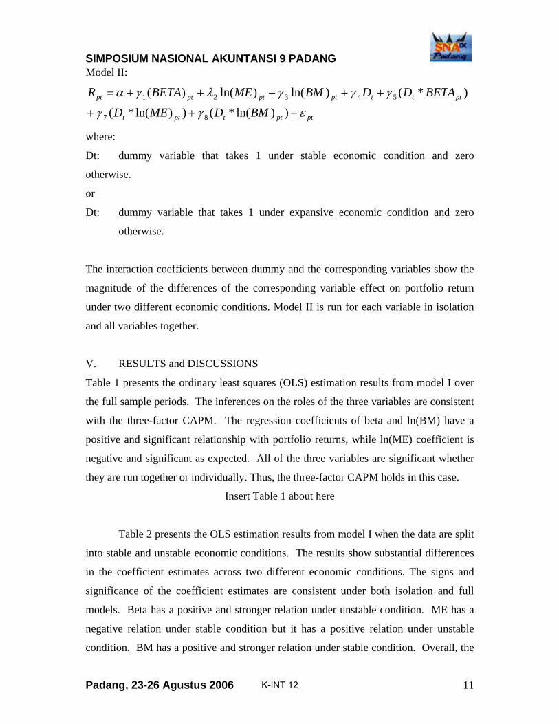
Model II:

ptpttptt

ptttptptptpt

BMDMED

BETADDBMMEBETAR

εγγ

γγγλγα

+++

+++++=

))ln(*())ln(*(

)*()ln()ln()(

87

54321

where:

Dt: dummy variable that takes 1 under stable economic condition and zero

otherwise.

or

Dt: dummy variable that takes 1 under expansive economic condition and zero

otherwise.

The interaction coefficients between dummy and the corresponding variables show the

magnitude of the differences of the corresponding variable effect on portfolio return

under two different economic conditions. Model II is run for each variable in isolation

and all variables together.

V. RESULTS and DISCUSSIONS

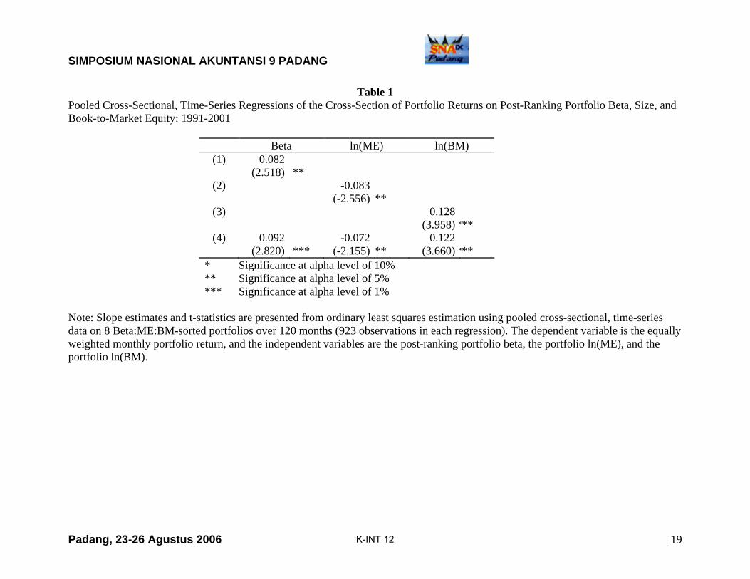
Table 1 presents the ordinary least squares (OLS) estimation results from model I over

the full sample periods. The inferences on the roles of the three variables are consistent

with the three-factor CAPM. The regression coefficients of beta and ln(BM) have a

positive and significant relationship with portfolio returns, while ln(ME) coefficient is

negative and significant as expected. All of the three variables are significant whether

they are run together or individually. Thus, the three-factor CAPM holds in this case.

Insert Table 1 about here

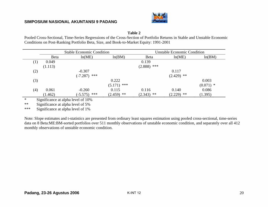
Table 2 presents the OLS estimation results from model I when the data are split

into stable and unstable economic conditions. The results show substantial differences

in the coefficient estimates across two different economic conditions. The signs and

significance of the coefficient estimates are consistent under both isolation and full

models. Beta has a positive and stronger relation under unstable condition. ME has a

negative relation under stable condition but it has a positive relation under unstable

condition. BM has a positive and stronger relation under stable condition. Overall, the

K-INT 12



three risk premium variables behave differently under stable and unstable conditions.

This result supports H1, that is, the economic conditions (stable and unstable) influence

the relationships of beta, ME, and BM with portfolio returns.


Under stable condition, in both isolation or full model, beta has no significant

relation, ME has a negative and significant relation, and BM has a positive and

significant relation with portfolio return. Except beta, ME and BM have a relation

consistent with three-factor CAPM. ME and BM seem to dominate in explaining the

cross-sectional variation in portfolio returns. Under unstable condition, beta has a

positive and significant relation, ME has positive and significant relation, and BM has

positive and significant relation with portfolio returns. Except ME, beta and BM have

a relation consistent with three factor CAPM.


Table 3 provides statistical evidence on the differences in the slope estimates. In

isolation, the interaction terms of D*beta and D*ln(ME) confirm the results shown in

Table 2. Beta has a weaker relation under stable condition, and ME coefficient is

significantly lower under stable condition. However, the interaction term of D*lnBM

does not confirm the differences shown in Table 2.

The full model shows that all three variables (beta, ME, and BM) are

significantly related to stock returns. However, the interaction terms of the full model

show different results, none of them are significant. The inconsistent results may be

due to existence of multicollinearity between interaction terms. Multiple steps of full

model regressions has to be done to avoid the multicollinearity between interaction

terms. All the reported coefficient estimates correspond to the variable that is the latest

entered in the model. Thus, there is a great possibility that the interaction term would no

longer be significant. The full model with interaction terms may not be the best model

in this case. Consequently, the magnitudes of the differences cannot be statistically

tested even though through observations from Table 2, there is an indication of

K-INT 12



differences. Therefore, the results of this study confirm that the relation of beta, ME,

and BM with portfolio returns are different under stable and unstable economic

conditions but the magnitudes of the differences cannot be observed.


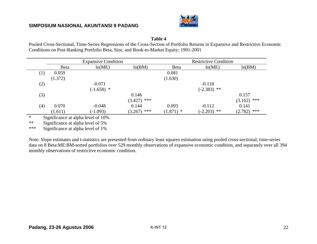
Table 4 presents the OLS estimation results from model I when the data are split

into expansive and restrictive economic conditions. The signs and significance of the

coefficient estimates are consistent under isolation or full model. Unlike the results

presented under stable and unstable economic conditions, the regressions of the sample

separated using expansive and restrictive economic conditions do not show substantial

differences in the coefficient estimates . In isolation, in both condition beta has no

significant relation, ME has a negative relation, and BM has a positive relation with

portfolio returns. The similar relations hold in the full model under both conditions.

Some points are worth to note that, firstly, the three-factor CAPM more strongly

hold in the restrictive condition, that all the three variables have relations and signs as

predicted by the three-factor CAPM. Secondly, under restrictive economic condition,

variables ME and BM seem to dominate in explaining the variation of portfolio returns.


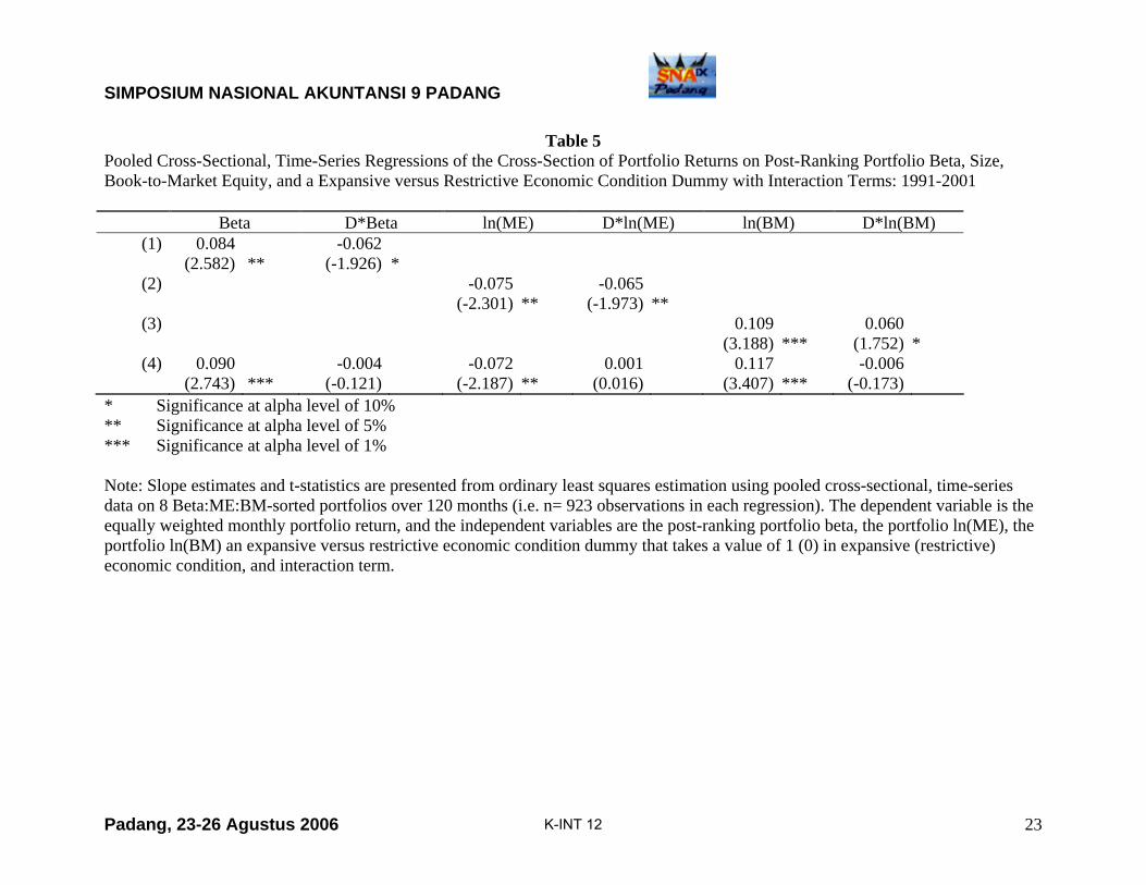
Table 5 provides statistical evidence on the differences in the slope estimates.

However, the results shown in Table 5 are inconsistent with those of shown in Table 4.

The results of the regression for the interaction term of each variable under isolation do

not conform with the results presented in Table 4. The same problem found for the

regression under the full model that a multicollinearity exists between interaction terms.

Multiple steps of full model regressions has to be done to avoid the multicollinearity

between interaction terms. All the reported coefficient estimates correspond to the

variable that is the latest entered in the model. The full model shows that all three

variables (beta, ME, and BM) are significantly related to stock returns, but none of the

interaction terms is significant. Therefore, the results of this study cannot provide a

K-INT 12



sufficient evidence to support H2, that is, the economic conditions (expansive and

restrictive) influence the relationships of beta, ME, and BM with portfolio returns.

Of the results, it is shown that the proposed economic state variable that can

separate the economic condition into expansive and restrictive conditions, cannot

robustly be used to identify the time varying risk premium of the three-factor CAPM.

However, the time varying of risk premiums attached in three-factor CAPM is indicated

by the regression results using stable and unstable economic condition separation.

Fama’s and French’s (1995) claim that ME and BM variables in three-factor CAPM can

capture the economic state variables may not be true. Thus, the search of the state

variables for inter-temporal CAPM has not come to an end.

VI. CONCLUSIONS and LIMITATIONS

This study re-examine the relations between the cross-section returns and three-factor

CAPM - beta, size, and book-to-market equity. The test result using the full sample

confirms that the three-factor CAPM holds in this case. In fact, the primary interest of

this study is to link the three-factor CAPM with the dynamic feature of inter-temporal

CAPM. The risk premiums associated with the three-factor CAPM are observed,

whether they behave differently under different economic conditions.

The use of common ex-post economic condition for separating the sample into

two different conditions enable us to observe different behavior of the risk premiums

associated with the three-factor CAPM. The use of Indonesian data from the periods of

1991 to 2001 make the partition of the sample into two different economic conditions

possible, namely, stable condition from the periods 1991 to 1997 and unstable

conditions from the rest of the periods. The result indicates that the risk premiums

associated with the three-factor CAPM do vary in stable and unstable economic

conditions, but the magnitudes cannot be observed in this study due to some statistical

problems. Thus, Fama’ and French’ (1995) claim that the ME and BM variables can

capture the macro economic state variables may not be true in this case.

The economic state variable, the growth of change in money supply, proposed

in this study fails to capture the time varying risk premiums attached in three-factor

CAPM. However, the ex-post economic state variable used in this study, stable and

K-INT 12



unstable economic conditions, can capture the time varying risk premiums represented

by the differences in relation of beta, ME, and BM with the cross-sectional variation in

portfolio returns under stable and unstable economic conditions. Thus, the search of the

state economic variables that ties the time varying risk premiums attached in three-

factor CAPM and Merton’s (1973) inter-temporal CAPM is worth to continue for future

studies. Overall, the evidence supports the link between three factor CAPM and inter-

temporal CAPM. A simple ex-ante measure of state variable should be found to capture

inter-temporal variation in expected stock returns.

K-INT 12



REFERENCES

Asri Marwan Sw, 2002, Size Effect and Stock Behavior During The Expansion and

Contraction Phases of Economic Cycle (An Empirical Evidence from Indonesian Stock Market), Simposium Nasional Keuangan In Memoriam Prof. Bambang Riyanto, 32-42.

Banz, R.W., 1981, The Relationship Between Return and Market Value of Common

Stock, Journal of Financial Economics 9: 3-18. Basu, S., 1983, The Relationship Between Earnings Yield, Market Value and Return for

NYSE Common Stock: Further Evidence, Journal of Financial Economics June:129-56.

Bodie, Zvi, Alex Kane, Alan J. Marcus, 2002, Investment, McGraw-Hill Irwin Bollerslev, T., 1986, Generalised Autoregressive Conditional Hetroscedasticity, Journal

of Econometrics 31: 307-327. Breeden, D.T, 1979. An Intertemporal Asset Pricing Model with Stochastic

Consumption and Investment Opportunities. Journal of Financial Economics 7: 265-96.

Brennan, Michael J., Tarun Chordia, Avanidhar Subrahmanyam, 1998, Alternative

Faktor Specifications, Security Characteristics, and the Cross-Section of Expected Returns, Journal of Financial Economics, 345-373

Brigham, Eugene F., Louis C. Gapenski, Philip R. Daves, 1999, Intermediate Financial

Management, Sixth Edition, The Dryden Press Chamberlain, G. and M. Rothschild, 1983. Arbitrage Factor Structure and Mean

Variance Analysisi on Large Asset Markets. Econometrica 51: 1281-1034. Chan, K.C. and Nai-Fu Chen, 1991, Structural and Return Characteristic of Small and

Large Firms, Journal of Finance 46: 739-1789. Chan, K.C., N. Jagedeesh, and J.Lakonishok, 1995. Evaluating the Performace of

Value Stocks versus Glamour Stocks: The Impact of Selection Bias, Journal of Financial Economics 38: 269-96.

Chen, N.F., 1991, Financial Investment Opportunities and The Macroeconomy, Journal

of Finance 46: 529-54. Elton, Edwin J., Martin J. Gruber, 1995, Modern Portfolio Theory and Investment

Analysis, Fifth Edition, John Wiley and Sons

K-INT 12



Engle, R.F., 1982, Autoregressive Conditional Hetroscedasticity with Estimates of UK

Inflation, Econometrica 50: 987-1007. Fama, E.F. and K.R. French, 1989, Business Conditions and Expected Returns on

Stocks and Bonds, Journal of Financial Economics 25: 3-25. Fama, E.F. and K.R. French, 1992, The Cross-Section of Expected Stock Returns,

Journal of Finance 47: 427-65. Fama, E.F. and K.R. French, 1995, Size and Book-to-Market Factors in Earnings and

Returns, Journal of Finance 50: 131-56. French, K.R., G.W. Schwert, and R.F. Stambaugh, 1987. Expected Stock Return and

Volatility. Journal of Financial Economics 19:329. Gertler, Mark and Simon Gilchrist, 1994, Monetary Policy, Business Cycles, and the

Behavior of Small Manufacturing Firms, Quartely Journal of Economics 109, 310-38.

Hadinugroho, Bambang, 2002, Pengaruh Beta, Size dan Book-to-market Equity dan

Earning Yield Terhadap Return Saham, Gadjah Mada University: Thesis. Huberman, Gur, and Shmuel Kandel, 1987, Mean-Variance Spanning, Journal of Finance 42: 873-888. Jensen, G.R., and J.M. Mercer, 2002, Monetary Policy and The Cross-Section of

Expected Stock Return, The Journal of Financial Research XXV: 125-39. Jensen, G.R., J.M. Mercer, and R.R. Johnson, 1996, Business Conditions, Monetary

Policy, and Expected Security Returns, Journal of Financial Economics 40: 213-37. Keim, D.B. and R.F. Stambaugh, 1986. Predicting Returns in Stock and Bond Markets.

Journal of Financial Economics 17: 357-90. Korajczyk, R. and C. Viallet, 1989 An Empirical Investigation of International Asset

Pricing. Review of Financial Studies 2: 553-85. Lehman, Bruce and David M Modest, 1988. The Empirical Foundation of the arbitrage

Pricing Theory. Journal of Financial Economics 21: 213-254. Lewellen, Jonathan, 1999, The Time-Series Relations Among Expected Return, Risk

dan Book-to-Market, Journal of Financial Economics, 5-43.

K-INT 12



Liew, J. and M. Vassalou, 2000. Can Book-to-Market, Size, and Momentum be Risk Factors That Predict Economic Growth? Journal of Financial Economics 57: 221-246.

Markowitz, Harry, 1959. Portfolio Selection: Efficient Diversification of Investment.

New York: Wiley. Merton, R.C., 1973. An Intertemporal Capital Asset Pricing Model. Econometrica 41:

867-87. Poerwanto, H., 2001, Analisis Hubungan Beta-Realized Return di BEJ Perioda 1994-

2000 : Pendekatan model kondisional , Gadjah Mada University: Thesis. Huberman, Gur, 1982. Arbitrage Pricing Theory, A Simple Approach. Journal of

Economic Theory 28: 183-98. Ross, Stephen A, 1976. An Arbitrage Theory of Capital Asset Pricing. Journal of

Economic Theory 13: 341-360. Sharpe, W.F., and Cooper, G.M., 1972, Risk-Return Class of New York Stock

Exchange Common Stocks, 1931-1967, Financial Analysts Journal, March-April, pp.46-52.

Solnik, R.E. , 1974. An Equilibrium Model of the International Capital Market. Journal

of Economic Theory 8: 500-24. Tobin, J.,1958. Liquidity Preferences as Behaviour Towards Risk. Review of Economic Studies 25: 65-86. Vassalou. M, 2002. News about Future GDP Growth as A Risk Factor in Equity Returns. Journal of Financial Economics 58: 221-246 Von Neuman, John and O. Margenstern, 1953. Theory of Games and Economic Behaviour. 3rd (ed), Princenton: Princenton University Press.

K-INT 12


Table 1 Pooled Cross-Sectional, Time-Series Regressions of the Cross-Section of Portfolio Returns on Post-Ranking Portfolio Beta, Size, and Book-to-Market Equity: 1991-2001

Beta ln(ME) ln(BM) (1)

(2)

(3)

(4)

0.082(2.518)

0.092(2.820)

** ***

-0.083(-2.556)

-0.072(-2.155)

** **

0.128 (3.958)

0.122 (3.660)

***

*** * Significance at alpha level of 10% ** Significance at alpha level of 5% *** Significance at alpha level of 1%

Note: Slope estimates and t-statistics are presented from ordinary least squares estimation using pooled cross-sectional, time-series data on 8 Beta:ME:BM-sorted portfolios over 120 months (923 observations in each regression). The dependent variable is the equally weighted monthly portfolio return, and the independent variables are the post-ranking portfolio beta, the portfolio ln(ME), and the portfolio ln(BM).

Padang, 23-26 Agustus 2006 19K-INT 12


Table 2 Pooled Cross-Sectional, Time-Series Regressions of the Cross-Section of Portfolio Returns in Stable and Unstable Economic Conditions on Post-Ranking Portfolio Beta, Size, and Book-to-Market Equity: 1991-2001 Stable Economic Condition Unstable Economic Condition Beta ln(ME) ln(BM) Beta ln(ME) ln(BM)

(1)

(2)

(3)

(4)

0.049 (1.113)

0.061 (1.462)

-0.307(-7.287)

-0.260(-5.575)

*** ***

0.222(5.171)

0.115(2.459)

*** **

0.139(2.888)

0.116(2.343)

*** **

0.117(2.429)

0.140(2.229)

** **

0.003(0.071)

0.086(1.395)

*

* Significance at alpha level of 10% ** Significance at alpha level of 5% *** Significance at alpha level of 1% Note: Slope estimates and t-statistics are presented from ordinary least squares estimation using pooled cross-sectional, time-series data on 8 Beta:ME:BM-sorted portfolios over 511 monthly observations of unstable economic condition, and separately over all 412 monthly observations of unstable economic condition.



Table 3 Pooled Cross-Sectional, Time-Series Regressions of the Cross-Section of Portfolio Returns on Post-Ranking Portfolio Beta, Size, Book-to-Market Equity, and a Stable versus Unstable Economic Condition Dummy with Interaction Terms: 1991-2001 Beta D*Beta ln(ME) D*ln(ME) ln(BM) D*ln(BM)

(1)

(2)

(3)

(4)

0.083 (2.529)

0.086 (2.587)

** **

-0.073(-2.212)

0.016(0.472)

**

-0.102(-3.127)

-0.070(-2.127)

*** **

-0.122(-3.746)

-0.029(-0.864)

***

0.151(3.039)

0.089(1.763)

*** *

-0.004(-0.079)

-0.053(-1.060)

* Significance at alpha level of 10% ** Significance at alpha level of 5% *** Significance at alpha level of 1% Note: Slope estimates and t-statistics are presented from ordinary least squares estimation using pooled cross-sectional, time-series data on 8 Beta:ME:BM-sorted portfolios over 120 months (i.e. n= 923 observations in each regression). The dependent variable is the equally weighted monthly portfolio return, and the independent variables are the post-ranking portfolio beta, the portfolio ln(ME), the portfolio ln(BM) a stable versus unstable economic condition dummy that takes a value of 1 (0) in stable (unstable) economic condition, and interaction term.



Table 4 Pooled Cross-Sectional, Time-Series Regressions of the Cross-Section of Portfolio Returns in Expansive and Restrictive Economic Conditions on Post-Ranking Portfolio Beta, Size, and Book-to-Market Equity: 1991-2001 Expansive Condition Restrictive Condition Beta ln(ME) ln(BM) Beta ln(ME) ln(BM)

(1)

(2)

(3)

(4)

0.059 (1.372)

0.070 (1.611)

-0.071(-1.658)

-0.048(-1.093)

*

0.146(3.427)

0.144(3.267)

*** ***

0.081(1.630)

0.093(1.871)

*

-0.118(-2.383)

-0.112(-2.203)

** **

0.157(3.162)

0.141(2.782)

*** ***

* Significance at alpha level of 10% ** Significance at alpha level of 5% *** Significance at alpha level of 1% Note: Slope estimates and t-statistics are presented from ordinary least squares estimation using pooled cross-sectional, time-series data on 8 Beta:ME:BM-sorted portfolios over 529 monthly observations of expansive economic condition, and separately over all 394 monthly observations of restrictive economic condition.



Table 5 Pooled Cross-Sectional, Time-Series Regressions of the Cross-Section of Portfolio Returns on Post-Ranking Portfolio Beta, Size, Book-to-Market Equity, and a Expansive versus Restrictive Economic Condition Dummy with Interaction Terms: 1991-2001 Beta D*Beta ln(ME) D*ln(ME) ln(BM) D*ln(BM)

(1)

(2)

(3)

(4)

0.084 (2.582)

0.090 (2.743)

** ***

-0.062(-1.926)

-0.004(-0.121)

*

-0.075(-2.301)

-0.072(-2.187)

** **

-0.065(-1.973)

0.001(0.016)

**

0.109(3.188)

0.117(3.407)

*** ***

0.060(1.752) -0.006

(-0.173)

*

* Significance at alpha level of 10% ** Significance at alpha level of 5% *** Significance at alpha level of 1% Note: Slope estimates and t-statistics are presented from ordinary least squares estimation using pooled cross-sectional, time-series data on 8 Beta:ME:BM-sorted portfolios over 120 months (i.e. n= 923 observations in each regression). The dependent variable is the equally weighted monthly portfolio return, and the independent variables are the post-ranking portfolio beta, the portfolio ln(ME), the portfolio ln(BM) an expansive versus restrictive economic condition dummy that takes a value of 1 (0) in expansive (restrictive) economic condition, and interaction term.


Documents

THE SEARCH OF ECONOMIC STATE VARIABLES FOR … · simposium nasional akuntansi 9 padang padang, 23-26 agustus 2006 1 the search of an economic state variable