Space Sci RevDOI 10.1007/s11214-013-9962-0

The Scientific Measurement System of the GravityRecovery and Interior Laboratory (GRAIL) Mission

Sami W. Asmar · Alexander S. Konopliv · Michael M. Watkins · James G. Williams ·Ryan S. Park · Gerhard Kruizinga · Meegyeong Paik · Dah-Ning Yuan ·Eugene Fahnestock · Dmitry Strekalov · Nate Harvey · Wenwen Lu · Daniel Kahan ·Kamal Oudrhiri · David E. Smith · Maria T. Zuber

Received: 5 October 2012 / Accepted: 22 January 2013© Springer Science+Business Media Dordrecht 2013

Abstract The Gravity Recovery and Interior Laboratory (GRAIL) mission to the Moon uti-lized an integrated scientific measurement system comprised of flight, ground, mission, anddata system elements in order to meet the end-to-end performance required to achieve itsscientific objectives. Modeling and simulation efforts were carried out early in the missionthat influenced and optimized the design, implementation, and testing of these elements.Because the two prime scientific observables, range between the two spacecraft and rangerates between each spacecraft and ground stations, can be affected by the performance ofany element of the mission, we treated every element as part of an extended science in-strument, a science system. All simulations and modeling took into account the design andconfiguration of each element to compute the expected performance and error budgets. Inthe process, scientific requirements were converted to engineering specifications that be-came the primary drivers for development and testing. Extensive simulations demonstratedthat the scientific objectives could in most cases be met with significant margin. Errors aregrouped into dynamic or kinematic sources and the largest source of non-gravitational er-ror comes from spacecraft thermal radiation. With all error models included, the baselinesolution shows that estimation of the lunar gravity field is robust against both dynamic andkinematic errors and a nominal field of degree 300 or better could be achieved according tothe scaled Kaula rule for the Moon. The core signature is more sensitive to modeling errorsand can be recovered with a small margin.

Keywords Gravity · Moon · Remote sensing · Spacecraft

Acronyms and AbbreviationsAGC Automatic Gain Control

S.W. Asmar (�) · A.S. Konopliv · M.M. Watkins · J.G. Williams · R.S. Park · G. Kruizinga · M. Paik ·D.-N. Yuan · E. Fahnestock · D. Strekalov · N. Harvey · W. Lu · D. Kahan · K. OudrhiriJet Propulsion Laboratory, California Institute of Technology, Pasadena, CA 91109, USAe-mail: sami.asmar@jpl.nasa.gov

D.E. Smith · M.T. ZuberDepartment of Earth, Atmospheric and Planetary Sciences, Massachusetts Institute of Technology,Cambridge, MA 02139-4307, USA

S.W. Asmar et al.

AMD Angular Momentum DesaturationC&DH Command & Data HandlerCBE Current Best EstimateCG Center of GravityCPU Central Processing UnitDSN Deep Space NetworkDOWR Dual One-way RangeECM Eccentricity Correction ManeuverEOP Earth Orientation PlatformET Ephemeris TimeGPS Global Positioning SystemGR-A GRAIL-A Spacecraft (Ebb)GR-B GRAIL-B Spacecraft (Flow)GRACE Gravity Recovery and Climate ExperimentGRAIL Gravity Recovery and Interior LaboratoryGSFC Goddard Space Flight CenterICRF International Celestial Reference FrameIERS International Earth Rotation and Reference Systems ServiceIR Infra RedIPU Instrument Processing Unit (GRACE mission)JPL Jet Propulsion LaboratoryKBR Ka-Band RangingKBRR Ka-Band Range-RateLGRS Lunar Gravity Ranging SystemLLR Lunar Laser RangingLOI Lunar Orbit InsertionLOS Line of SightLP Lunar ProspectormGal milliGal (where 1 Gal = 0.01 m s−2)MGS Mars Global SurveyorMIT Massachusetts Institute of TechnologyMOS Mission Operations SystemMIRAGE Multiple Interferometric Ranging and GPS EnsembleMMDOM Multi-mission Distributed Object ManagerMONTE Mission-analysis, Operations, and Navigation Toolkit EnvironmentMPST Mission Planning and Sequence TeamMRO Mars Reconnaissance OrbiterMWA Microwave AssemblyNASA National Aeronautics and Space AdministrationODP Orbit Determination ProgramOPR Orbital Period ReductionOSC Onboard Spacecraft ClocksOTM Orbit Trim ManeuverPDS Planetary Data SystemPM Primary MissionPPS Pulse Per SecondRSB Radio Science BeaconRSR Radio Science ReceiverSCT Spacecraft Team

The GRAIL Scientific Measurement System

SDS Science Data SystemSIS Software Interface SpecificationSRIF Square Root Information FilterSRP Solar Radiation PressureTAI International Atomic TimeTCM Trajectory Correction ManeuverTDB Barycentric Dynamic TimeTDS Telemetry Delivery SystemTDT Terrestrial Dynamic TimeTLC Trans-Lunar CruiseTSF Transition to Science FormationTSM Transition to Science ManeuverTTS Time Transfer SystemUSO Ultra-stable OscillatorUTC Universal Time CoordinatedVLBI Very Long Baseline Interferometry

1 Introduction and Heritage

The Gravity Recovery and Interior Laboratory (GRAIL) mission is comprised of two space-craft, named Ebb and Flow, flying in precision formation around the Moon. The mission’spurpose is to recover the lunar gravitational field in order to investigate the interior structureof the Moon from the crust to the core. The spacecraft were launched together on Septem-ber 10, 2011 and began science operations and data acquisition on March 1, 2012. Zuberet al. (2013, this issue) presents an overview of the mission including scientific objectivesand measurement requirements. Klipstein et al. (2013, this issue) describes the design andimplementation of the GRAIL payload. Hoffman (2009) described GRAIL’s flight systemand Roncoli and Fujii (2010) described the mission design.

This paper illustrates how a team of scientists and engineers prepared to meet GRAILscientific objectives and data quality requirements through simulations and modeling of thedesign and configuration of the flight and ground systems. It details dynamic and kinematicmodels for estimating error sources in the form of non-gravitational forces and how thesemodels were applied, along with the lunar gravity model, to elaborate computer simulationsin the context of an integrated scientific measurement system. This paper also documents themethods, tools, and results of the simulations. This work was carried out at the Jet PropulsionLaboratory (JPL) prior to the science orbital phase and reviewed by expert peers from differ-ent institutions; the knowledge is based on the combined experiences of the team memberswith gravity observations on numerous planetary missions. This effort demonstrated that themission was capable of meeting the science requirements as well as paved the way to theoperational tools and procedures for the actual science data analysis.

The GRAIL concept was derived from the Gravity Recovery and Climate Experiment(GRACE) Earth mission and utilized a modified GRACE payload called the Lunar GravityRanging System (LGRS); the GRAIL and GRACE spacecraft are unrelated. For an overviewof the GRACE mission see Tapley et al. (2004a, 2004b); for a description of the GRACEpayload, see Dunn et al. (2003); and for error analysis in the GRACE system and measure-ments, see Kim and Tapley (2002).

Despite the high heritage, there are significant differences between the GRAIL andGRACE science payloads, listed in Table 1. GRACE is equipped with a Global Positioning

S.W. Asmar et al.

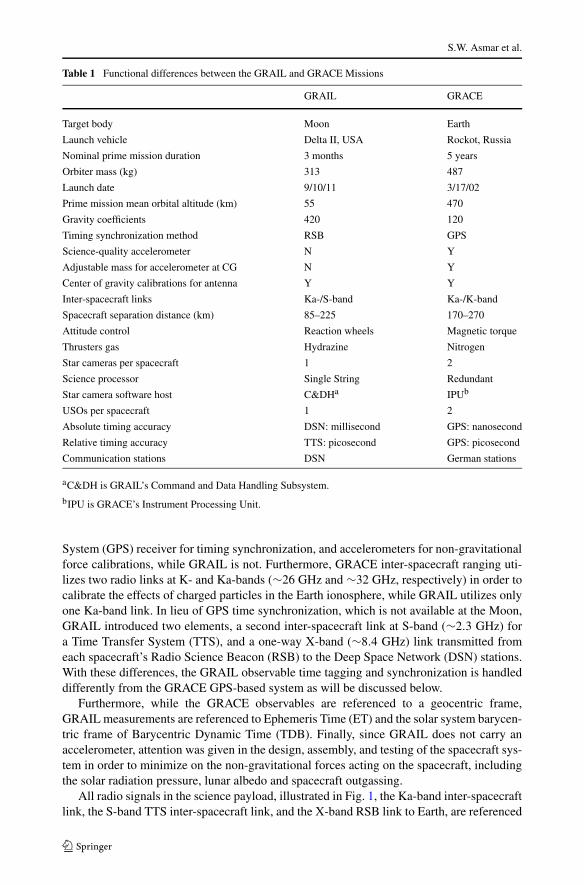
Table 1 Functional differences between the GRAIL and GRACE Missions

GRAIL GRACE

Target body Moon Earth

Launch vehicle Delta II, USA Rockot, Russia

Nominal prime mission duration 3 months 5 years

Orbiter mass (kg) 313 487

Launch date 9/10/11 3/17/02

Prime mission mean orbital altitude (km) 55 470

Gravity coefficients 420 120

Timing synchronization method RSB GPS

Science-quality accelerometer N Y

Adjustable mass for accelerometer at CG N Y

Center of gravity calibrations for antenna Y Y

Inter-spacecraft links Ka-/S-band Ka-/K-band

Spacecraft separation distance (km) 85–225 170–270

Attitude control Reaction wheels Magnetic torque

Thrusters gas Hydrazine Nitrogen

Star cameras per spacecraft 1 2

Science processor Single String Redundant

Star camera software host C&DHa IPUb

USOs per spacecraft 1 2

Absolute timing accuracy DSN: millisecond GPS: nanosecond

Relative timing accuracy TTS: picosecond GPS: picosecond

Communication stations DSN German stations

aC&DH is GRAIL’s Command and Data Handling Subsystem.

bIPU is GRACE’s Instrument Processing Unit.

System (GPS) receiver for timing synchronization, and accelerometers for non-gravitationalforce calibrations, while GRAIL is not. Furthermore, GRACE inter-spacecraft ranging uti-lizes two radio links at K- and Ka-bands (∼26 GHz and ∼32 GHz, respectively) in order tocalibrate the effects of charged particles in the Earth ionosphere, while GRAIL utilizes onlyone Ka-band link. In lieu of GPS time synchronization, which is not available at the Moon,GRAIL introduced two elements, a second inter-spacecraft link at S-band (∼2.3 GHz) fora Time Transfer System (TTS), and a one-way X-band (∼8.4 GHz) link transmitted fromeach spacecraft’s Radio Science Beacon (RSB) to the Deep Space Network (DSN) stations.With these differences, the GRAIL observable time tagging and synchronization is handleddifferently from the GRACE GPS-based system as will be discussed below.

Furthermore, while the GRACE observables are referenced to a geocentric frame,GRAIL measurements are referenced to Ephemeris Time (ET) and the solar system barycen-tric frame of Barycentric Dynamic Time (TDB). Finally, since GRAIL does not carry anaccelerometer, attention was given in the design, assembly, and testing of the spacecraft sys-tem in order to minimize on the non-gravitational forces acting on the spacecraft, includingthe solar radiation pressure, lunar albedo and spacecraft outgassing.

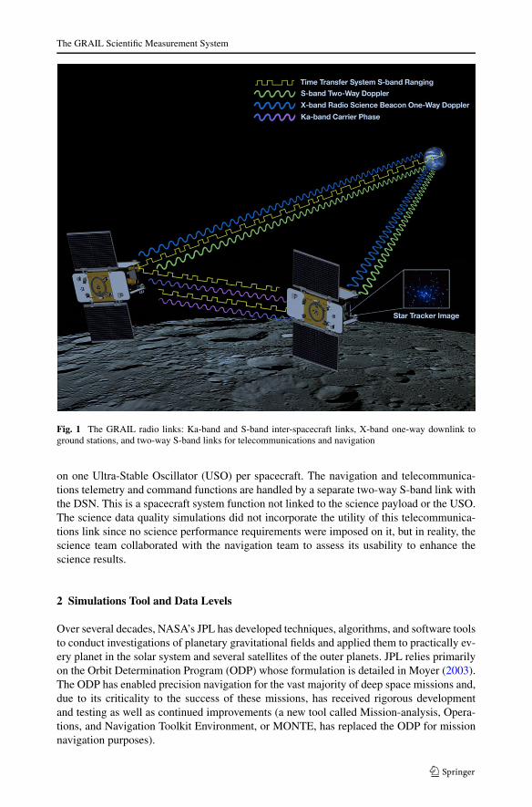
All radio signals in the science payload, illustrated in Fig. 1, the Ka-band inter-spacecraftlink, the S-band TTS inter-spacecraft link, and the X-band RSB link to Earth, are referenced

The GRAIL Scientific Measurement System

Fig. 1 The GRAIL radio links: Ka-band and S-band inter-spacecraft links, X-band one-way downlink toground stations, and two-way S-band links for telecommunications and navigation

on one Ultra-Stable Oscillator (USO) per spacecraft. The navigation and telecommunica-tions telemetry and command functions are handled by a separate two-way S-band link withthe DSN. This is a spacecraft system function not linked to the science payload or the USO.The science data quality simulations did not incorporate the utility of this telecommunica-tions link since no science performance requirements were imposed on it, but in reality, thescience team collaborated with the navigation team to assess its usability to enhance thescience results.

2 Simulations Tool and Data Levels

Over several decades, NASA’s JPL has developed techniques, algorithms, and software toolsto conduct investigations of planetary gravitational fields and applied them to practically ev-ery planet in the solar system and several satellites of the outer planets. JPL relies primarilyon the Orbit Determination Program (ODP) whose formulation is detailed in Moyer (2003).The ODP has enabled precision navigation for the vast majority of deep space missions and,due to its criticality to the success of these missions, has received rigorous developmentand testing as well as continued improvements (a new tool called Mission-analysis, Opera-tions, and Navigation Toolkit Environment, or MONTE, has replaced the ODP for missionnavigation purposes).

S.W. Asmar et al.

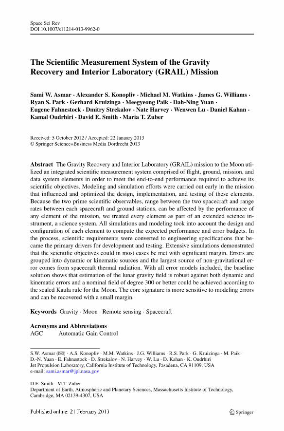
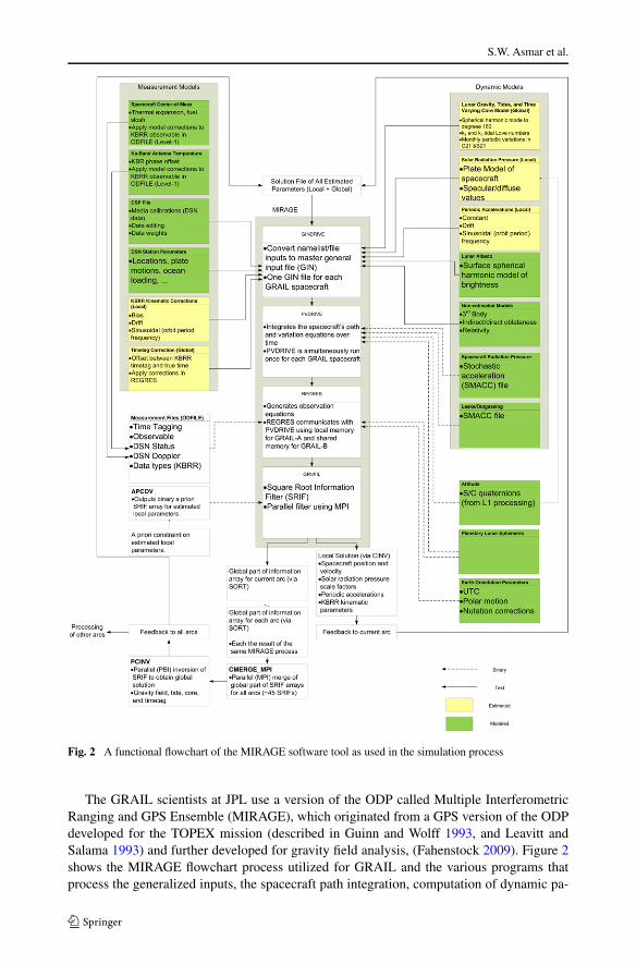
Fig. 2 A functional flowchart of the MIRAGE software tool as used in the simulation process

The GRAIL scientists at JPL use a version of the ODP called Multiple InterferometricRanging and GPS Ensemble (MIRAGE), which originated from a GPS version of the ODPdeveloped for the TOPEX mission (described in Guinn and Wolff 1993, and Leavitt andSalama 1993) and further developed for gravity field analysis, (Fahenstock 2009). Figure 2shows the MIRAGE flowchart process utilized for GRAIL and the various programs thatprocess the generalized inputs, the spacecraft path integration, computation of dynamic pa-

The GRAIL Scientific Measurement System

rameter partials, and the data observables. This figure documents the necessary interfacesbetween the software elements and input/output files as well as the relevant computationalparameters and has been a key figure for the simulations peer-review process. There are threesubsets of programs that integrate the spacecraft motion, process the spacecraft observationsand filter or estimate the spacecraft state and related parameters using the observations.

To determine the spacecraft dynamical path, the program numerically integrates thespacecraft Cartesian state by including all known forces acting on the spacecraft, suchas gravity, solar pressure, lunar albedo, and spacecraft thrusting. The spacecraft state andthe force model partial derivatives (e.g., gravity harmonics) that are later estimated areintegrated using the variable order Adams method described in Krogh (1973). The non-rotating International Celestial Reference Frame (ICRF) defines the inertial coordinate sys-tem, which is nearly equal to the Earth’s mean equator and equinox at the epoch of J2000.

The GRAIL data are categorized in 3 levels, also shown in of Zuber et al. (2013, thisissue). Level 0 is the raw data acquired by the spacecraft science payload, the LGRS, andDSN Doppler. Level 1 is the expanded, edited and calibrated data. Level 1 processing is theconversion from Level 0 files to Level 1 files. Level 1 processing also applies a time tagconversion, time of flight correction, and phase center offset, as well as generates instan-taneous range-rate and range-acceleration observables by numerical differentiation of thebiased range observables. Level 2 is the gravity field spherical harmonic expansion; level 2processing refers to the production of Level 2 data. The simulations described herein emu-late the generation of Levels 1 and 2 GRAIL mission data.

3 Gravity Model Representation

Gravitational fields provide a key tool for probing the interior structure of planets. The lunargravity, when combined with topography, leads to geophysical models that address impor-tant phenomena such as the structure of the crust and lithosphere, the asymmetric lunarthermal evolution, subsurface structure of impact basins and the origin of mascons, and thetemporal evolution of crustal brecciation and magmatism. Long-wavelength gravity mea-surements can place constraints on the presence of a lunar core.

A gravitational field represents variations in the gravitational potential of a planet andgravity anomalies at its surface. It can be mathematically represented via coefficients of aspherical harmonic expansion whose degree and order reflect the surface resolution. A fieldof degree 180, for example, represents a half-wavelength, or spatial block size, surface reso-lution of 30 km; for degree n, the resolution is 30×180/n km. The gravitational potential inspherical harmonic form is represented in the body-fixed reference frame with normalizedcoefficients (Cnm, Snm) is represented after Heiskanen and Moritz (1967) and Kaula (1966)as:

U = GM

r+ GM

r

∞∑

n=1

n∑

m=0

(Re

r

)n

P nm(sinϕlat )[Cnm cos(mλ) + Snm sin(mλ)

](1)

G is the gravitational constant, M is the mass of the central body, r is the radial distancecoordinate, m is the order, P nm are the fully normalized associated Legendre polynomials,Re is the reference radius of the body, ϕlat is the latitude, and λ is the longitude. The gravitycoefficients are normalized so that the integral of the harmonic squared equals the area ofa unit sphere, and are related to the un-normalized coefficients by Kaula (1966), where δ is

S.W. Asmar et al.

the Kronecker delta:(

Cnm

Snm

)=

[(n − m)!(2n + 1)(2 − δ0m)

(n + m)!]1/2(

Cnm

Snm

)= fnm

(Cnm

Snm

)(2)

There exist singularities at the pole in the partials of the gravity acceleration with respect tothe spacecraft position when using the Legendre polynomials as a function of latitude. Toaccommodate this, MIRAGE uses a nonsingular formulation of the gravitational potential,including recursion relations given by Pines (1973), in calculation of the acceleration andpartials.

The gravitational potential also accounts for tides caused by a perturbing body. Thesecond-degree tidal potential acting on a satellite at position �r relative to the central body,with the perturbing body (e.g., Sun and Earth for GRAIL) at position �rp , is:

U = k2GMp

R

R6

r3r3p

[3

2(r · rp)2 − 1

2

](3)

where k2 is the second degree potential Love number, Mp is the mass of the perturbing bodycausing the tide, and R is the equatorial radius of the central body. Tides raised on the Moonby the Sun are two orders-of-magnitude smaller than tides raised by the Earth. The acceler-ation due to constant lunar tides is modeled using a spherical harmonics representation:

�Cnm − i�Snm = knm

2n + 1

∑

j

GMj

GM

Rn+1M

rn+1mj

Pnm(sinϕj )e−imλj (4)

Simplifying, the non-dissipative tides contribute time-varying components to second degreeand order normalized coefficients as follows (McCarthy and Petit 2003):

�J 2 = −k20

√1

5

GMpR3

GMr3p

[3

2sin2 ϕp − 1

2

]

�C21 = k21

√3

5

GMpR3

GMr3p

sinϕp cosϕp cosλp

�S21 = k21

√3

5

GMpR3

GMr3p

sinϕp cosϕp sinλp (5)

�C22 = k22

√3

20

GMpR3

GMr3p

cos2 ϕp cos 2λp

�S22 = k22

√3

30

GMpR3

GMr3p

cos2 ϕp sin 2λp

Here, ϕp and λp are the latitude and longitude of the perturbing body on the surface ofthe central body. Separate Love numbers have been used for each order, though they are ex-pected to be equal (k20 = k21 = k22). Degree-3 Love number solutions have been investigatedand their effect is barely detectable.

The tidal potential consists of a variable term and a constant or permanent term. De-pending on choice of convention, the constant term may or may not be included in thecorresponding gravity coefficient. The MIRAGE-generated gravity fields do not include the

The GRAIL Scientific Measurement System

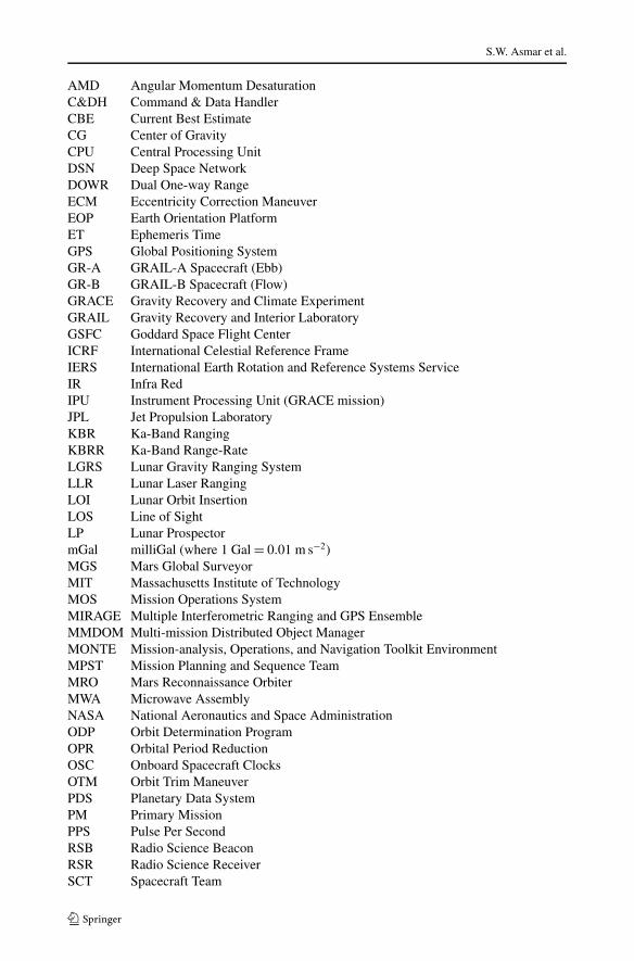
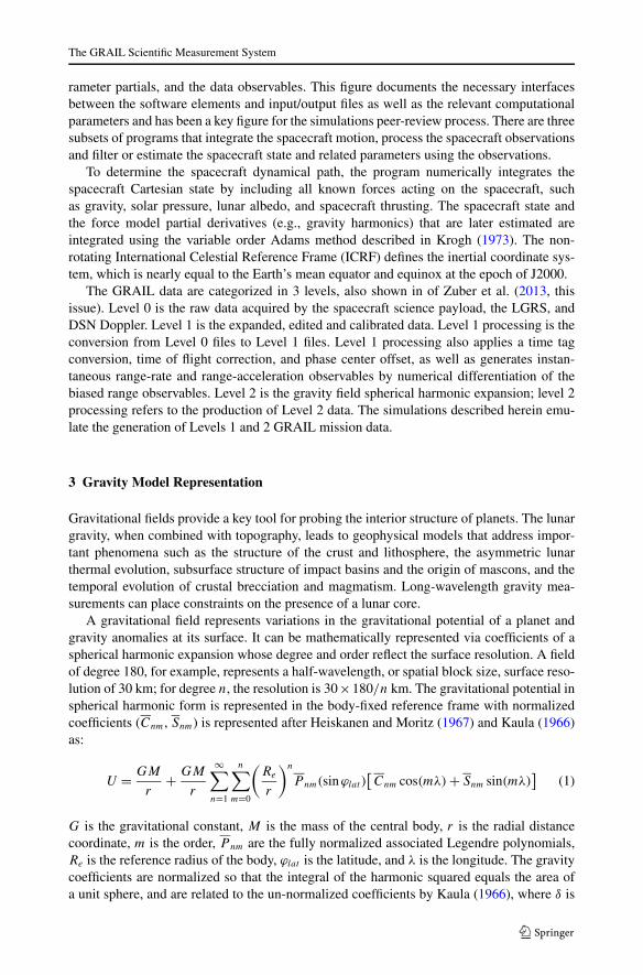
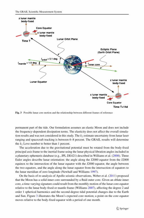
Fig. 3 Possible lunar core motion and the relationship between different frames of reference

permanent part of the tide. Our formulation assumes an elastic Moon and does not includethe frequency-dependent dissipation terms. The elasticity does not affect the overall simula-tion results and was not considered in this study. The k2 estimate uncertainty from lunar laserranging and spacecraft tracking is between 6–8 percent. The GRAIL results will determinethe k2 Love number to better than 1 percent.

The acceleration due to the gravitational potential must be rotated from the body-fixedprincipal axis frame to the inertial frame using the lunar physical libration angles included ina planetary ephemeris database (e.g., JPL DE421) described in Williams et al. (2008). ThreeEuler angles describe lunar orientation: the angle along the J2000 equator from the J2000equinox to the intersection of the lunar equator with the J2000 equator, the angle betweenthe two equators, and the angle along the lunar equator from the intersection of equators tothe lunar meridian of zero longitude (Newhall and Williams 1997).

On the basis of re-analysis of Apollo seismic observations, Weber et al. (2011) proposedthat the Moon has a solid inner core surrounded by a fluid outer core. Given an oblate innercore, a time-varying signature could result from the monthly motion of the lunar core equatorrelative to the lunar body-fixed or mantle frame (Williams 2007), affecting the degree 2 andorder 1 spherical harmonics and the second-degree tidal potential changes due to the Earthand Sun. Figure 3 illustrates the Moon’s expected core motion; a point on the core equatormoves relative to the body-fixed equator with a period of one month.

S.W. Asmar et al.

Due to the pole offset of the core and mantle frame, the core motion introduces a monthlysignature in the C21 and S21 gravity coefficients as follows:

�C21 = α21 cos(ωt + ϕ), (6)

�S21 = β21 cos(ωt + ϕ) (7)

where �C21,�S21 is the monthly gravitational potential oscillation due to a possible solidinner core with an axis of rotation tilted relative to the mantle’s axis, included in all simu-lations, ω is the frequency and ϕ is the phase of this periodic signature. For the latter, weassume a priori knowledge when estimating the amplitudes of the C21 and S21 signatures(α21 and β21) along with the gravity field and tidal Love number. If the inner core had anequilibrium figure for tide and spin distortion, then the ratio of amplitudes for C21 and S21

signatures would be 4. While this ratio is not assumed, it has been used to set requirementsfor amplitude uncertainties. We investigated both the uncertainty of the core amplitudes andthe differences of the estimated values with the a priori values. These estimated amplitudesplus the tidal Love numbers encapsulate the results of GRAIL’s science investigations ad-dressing the deep interior.

4 Model Estimation and Dynamical Integration

JPL’s gravity field estimation process relies on two primary data types: a link between thespacecraft and Earth, which is a one-way X-band link, and an inter-spacecraft link calledthe Ka-band Range (KBR). The latter’s first derivative, the Ka-band Range Rate (KBRR),precisely measures the relative movement of Ebb and Flow, which permits estimation of thelunar gravity field. The combined measurement of two sets of ranging data, one measuredby Ebb and a second by Flow, is called the Dual One-Way Range (DOWR) measurement.Ebb and Flow are tracked from Earth by the DSN, which produces Doppler data used todetermine the absolute position of each spacecraft:

zd = ρse · ρse, (8)

zs = ρba · ρba (9)

where ρse represents the vector from spacecraft to the DSN station and ρba represents thevector from Ebb to Flow.

The estimation of the gravity field follows the same steps as the orbit determinationprocess in navigation but involves many more parameters and methods that may constrainthe gravity field and other model parameters to obtain the most realistic solution. Althoughthe planetary gravity field solutions often require a Kaula power law constraint (Kaula 1966),the uniform and global coverage of the KBRR data does not require a constraint in oursimulations except for solutions of high degree (i.e., degree ∼270) where a small power-type constraint was applied.

Letting �r and �v be the position and velocity vectors of the spacecraft relative to the centralbody, the software integrates the second order differential equations

�r = �f (�r, �v, �q) = ∇U(�r) + �fpm + �fin-pm + �fin-obl + �fsrp + �falb + �fatt + �frel + · · · (10)

Here, �f (�r, �v, �q) is the total acceleration of the spacecraft and �q are all the constant ( �q = 0)model parameters to be estimated (e.g., gravity harmonic coefficients). Contributions to the

The GRAIL Scientific Measurement System

total acceleration include the acceleration of the spacecraft relative to the central body dueto the gravitational potential of the central body ∇U(�r), the spacecraft acceleration due toother solar system bodies treated as point masses �fpm, the indirect point mass accelerationof the central body in the solar system barycentric frame due to the other planets and naturalsatellites �fin-pm, the indirect oblateness acceleration of the central body (e.g., Moon) due toanother body’s oblateness (e.g., Earth) �fin-obl , the acceleration of the spacecraft due to solarradiation pressure �fsrp , the acceleration due to lunar albedo �falb , the acceleration due tospacecraft gas thrusting for attitude control maneuvers (usually for de-spinning angular mo-mentum wheels) �fatt , and the pseudo-acceleration due to general relativity corrections �frel .Other accelerations also exist and may include spacecraft thermal forces, infrared radiation,tides, and empirical, usually periodic, acceleration models. Specific acceleration models thathave been taken into account are described below.

4.1 Acceleration Due to Solar Radiation Pressure

Each spacecraft is modeled with five single-sided flat plates to model the acceleration due tosolar radiation pressure (SRP) as detailed in Fahnestock et al. (2012) and Park et al. (2012).For each plate, the acceleration is computed as:

asrp = CSs

msr2sp

(Fnun + Frus), (11)

Fn = −A(2κdvd + 4κsvs cosα) cosα, (12)

Fr = −A(1 − 2κsvs) cosα. (13)

The acceleration due to SRP is on the order of 10−10 km/s2. It is separable from the effectof gravity in the estimation process. With a ray-tracing technique to model self-shadowingon the spacecraft bus and on-board telemetry of the power system to detect entry and exitfrom lunar shadow, the SRP accelerations can be determined to a few percent level.

4.2 Acceleration Due to Spacecraft Thermal Radiation:

For a flat plate component, the acceleration due to spacecraft thermal re-radiation is:

astr = −2 × 10−6Aσsb

3mscεT 4un. (14)

This is used to convert from any given plate’s surface temperature to its accelerationcontribution.

4.3 Acceleration Due to Lunar Albedo and Thermal Emission

The element of acceleration on a spacecraft due to lunar radiation pressure from a point P

on the surface of the Moon can be computed (from Park et al. 2012) as:

dalrp = H(Fnun + Fr rps)cosψ

πr2ps

dAplanet . (15)

For reflected sunlight (albedo):

H = CSm cosψs

msr2ms

N∑

�=0

�∑

m=0

(CA

�m cosmλp + SA�m sinmλp

)P�m(sinϕp), (16)

S.W. Asmar et al.

and for thermal emission (infrared):

H = C

4msr2ms

N∑

�=0

�∑

m=0

(CE

�m cosmλp + SE�m sinmλp

)P�m(sinϕp). (17)

The albedo map is a constant field whereas the thermal map is a function of local lunartime because of topographic variation; the thermal map derived using the measurementsfrom Lunar Reconnaissance Orbiter’s Diviner Lunar Radiometer Experiment data. For thisreason, the following simplified thermal emission model was derived for the simulation ofthe total error budget:

H =⎧⎨

⎩

CσsbT 4max cosψs

4msr2csL

, if ψs ≤ 89.5◦,CσsbT 4

min4msr

2csL

, otherwise,(18)

where Tmax = 382.86 K and Tmin = 95 K. Thermal maps were computed at the local noon-time when the Sun is at 0◦ longitude and 0◦ latitude.

4.4 Acceleration Due to Un-modeled Forces

The acceleration due to un-modeled forces is used to represent the errors in the non-gravitational forces from solar pressure, spacecraft thermal radiation, lunar radiation, andspacecraft outgassing and is represented as the periodic acceleration formulation:

auf = (Pr + Cr1 cos θ + Cr2 cos 2θ + Sr1 sin θ + Sr2 sin 2θ)er

+ (Pt + Ct1 cos θ + Ct2 cos 2θ + St1 sin θ + St2 sin 2θ)et

+ (Pn + Cn1 cos θ + Cn2 cos 2θ + Sn1 sin θ + Sn2 sin 2θ)en, (19)

where er , et , and en represent the radial, transverse, and normal unit-vectors, respectivelyand θ denotes the angle from the ascending node of the spacecraft orbit on the EME2000plane to the spacecraft. The periodic acceleration is nominally set to zero in the initial tra-jectory integration and is used to estimate the errors in the non-gravitational accelerations.The terms Pi represent the constant accelerations during the time interval that the corre-sponding periodic acceleration model is active. The terms (Ci1, Si1) and (Ci2, Si2) representthe once-per-orbit and twice-per-orbit acceleration amplitudes, respectively.

In addition to integrating the spacecraft position and velocity, MIRAGE integrates thevariational equations to estimate the epoch state and constant parameters. Following nomen-clature in Tapley et al. (2004a, 2004b), the nominal trajectory is given by:

X∗(t) =⎛

⎝�r∗(t)�v∗(t)�q∗

⎞

⎠ . (20)

The first order differential equation to integrate in order to determine the nominal orbitis:

X∗(t) =⎛

⎝�v∗

�f (�r∗, �v∗, �q∗)0

⎞

⎠ = F(X∗, t

). (21)

The GRAIL Scientific Measurement System

The variation of the trajectory from its nominal path is x(t) = X(t) − X∗(t) and thelinearized equations:

x(t) = A(t)x(t) =(

∂F (t)

∂X(t)

)∗x(t) (22)

The integrated solution is the state transition matrix Φ(t, t0), which relates the deviationfrom the nominal path at epoch t0 to the deviation from the nominal path at time t for the 6position and velocity epoch parameters matrix (U6×6) and the p constant model parameters(V6×6):

x(t) = Φ(t, t0)x(t0) =[

U6×6 V6×6

0p×6 Ip×p

]x(t0). (23)

The second order differential equations that MIRAGE integrates for each GRAIL space-craft include the 3 position variables of Eq. (10), 18 variables representing the changes inposition and velocity due to small changes in epoch position and velocity which define thematrix U6×6, and three equations for each dynamic parameter or constant from being esti-mated. For a complete gravity field of degree and order n, the total number of gravity fieldparameters is given by (n − 1)(n + 3), or, for example, 32,757 parameters for a 180 degreeand order field.

5 Processing and Filtering of Observations

After numerical integration, MIRAGE processes Doppler and range observations. FollowingTapley et al. (2004a), the general form of the observation equation is

Y = G(X, t) + ε, (24)

where Y is the actual observation, G(X, t) is a mathematical expression to calculate themodeled observation value, and ε is the observation error. The DSN Doppler data is not aninstantaneous velocity measurement, but is processed in similar fashion to a range observ-able and is given by a differenced range measurement for two-way Doppler as

G(X, t) = ((r12 + r23)e − (r12 + r23)s

)/�t + · · · (25)

where r12 is the uplink range transmitted by the ground station and received at the space-craft, and r23 is the downlink range from the spacecraft to the earth station, with subscriptsdenoting the end and start of the Doppler count interval, �t . To process a Doppler obser-vation, we must solve the light time equation in a solar system barycentric frame, i.e., findthe original transmit time at the first station and the receive time at the spacecraft usingan iterative procedure. Equation (25) requires DSN calibrations for Earth ionospheric andtropospheric refraction (Mannucci et al. 1998), and corrections for relativistic propagationdelay due to the Sun and planets, solar plasma delays due to the solar corona of the Sun, andany measurement biases.

The dual one-way phase measurement between Ebb and Flow can be converted to abiased range, by an algorithm first developed by Kim (2000). Our lunar gravity recoveryprocess ingests instantaneous range-rate, modeled as a projection of the velocity differencevector, r12, along the line-of-sight unit vector,

�e12.

G(X, t) = ρ = r12 • �e12 (26)

S.W. Asmar et al.

Processing observables also requires the linearized form of Eq. (24). Given an observ-able Y , we compute a nominal observable Y ∗(t) based on an input nominal orbit, and cal-culate an observation residual y:

y = Y − Y ∗(t) (27)

Using the state transition matrix to map to the epoch time, Eq. (24) is then written as

y =(

∂G

∂X

)Φ(t, t0)x0 + ε = Hx0 + ε. (28)

Based on the vector of residuals y and partials matrix H , the MIRAGE filter solves for astate X that minimizes these ε error terms.

The calculation of the nominal DSN Doppler observable and related partials in Eq. (28)involves the precise location of the Earth station in a solar system barycentric ICRF frameas shown in Yuan et al. (2001). The Earth-fixed coordinate system is consistent with theInternational Earth Rotation and Reference Systems Service (IERS) terrestrial referenceframe labeled ITRF93 as shown in Boucher et al. (1994). The rotation of the Earth-fixedcoordinates of the DSN locations to the Earth centered inertial system requires a series ofcoordinate transformations due to precession as in the IAU 1976 model described in Lieskeet al. (1977) and nutation of the mean pole as in the IAU 1980 nutation theory described inWahr (1981) and Seidelmann (1982) plus daily corrections to the model from the JPL EarthOrientation Platform (EOP) product of Folkner et al. (1993), rotation of the Earth as in Aokiet al. (1982) and Aoki and Kinoshita (1983) and UTC-UT1R corrections of the JPL EOP file,and polar motion of the rotation axis. The JPL EOP product is derived from the Very LongBaseline Interferometry (VLBI) and Lunar Laser Ranging (LLR) observations and includesEarth rotation and polar motion calibrations and, in addition, nutation correction parametersnecessary to determine inertial station locations to the level of a few centimeters.

The body-fixed ITRF93 DSN station locations have been determined with VLBI mea-surements and conventional and GPS surveying. The coordinate uncertainties are about 4 cmfor DSN stations that have participated in regular VLBI experiments, and about 10 cm forother stations; Folkner (1996) also provides the antenna phase center offset vector for eachDSN station. These DSN station locations are consistent with the NNR-NEWVAL1 platemotion model (Argus and Gordon 1991). The variations of DSN station coordinates causedby solid Earth tide, ocean tide loading, and rotational deformation due to polar motion arecorrected according to the IERS standards for 1992 (McCarthy and Petit 2003).

Once the observation equations are found, MIRAGE estimates the spacecraft state andother parameters using a weighted Square Root Information Filter (SRIF), see Lawson andHanson (1995). SRIF computation time dominates MIRAGE processing, and for the largerplanetary gravity fields of the Moon we run on two Beowulf Linux clusters (a 28-nodemachine with 112 CPU cores and a 45-node machine with 360 CPU cores). In normal form,the least-squares solution is given by:

x = (HT WH + P −1

ap

)−1HT Wy (29)

W is the weight matrix for the observations and Pap is the a priori covariance matrix of theparameters being estimated. In the MIRAGE SRIF filter, the solution equation is kept in theform:

Rx = z (30)

The GRAIL Scientific Measurement System

R is the upper triangular square-root of the information array and R and z are related to thenormal equations as:

RT R = HT WH + P −1ap , (31)

z = (RT

)−1HT Wy (32)

and the covariance P of the solution (inverse of the information array) is given by:

P = R−1(R−1

)T(33)

We separate observations for gravity field determination into disjoint time spans calleddata arcs. Two-day-long data arcs are typical. The parameters estimated in the arc-by-arcgravity solutions consist of arc-dependent local variables: spacecraft state, solar radiationpressure coefficients, etc., and global variables common to all data arcs: gravity coefficients,tide parameters, etc. Merging the global parameter portion of a sequence of data arc squareroot information arrays produces a solution equivalent to solving for a single set of globalparameters plus independent arc-specific local parameters (Kaula 1966).

When solving for a large number of parameters, convergence is very sensitive to a priorivalues and uncertainties. If the spacecraft initial state is poorly known and a filter tries tosolve for both the trajectory and a high-resolution gravity field at the same time, the iterationmay never converge. In order to avoid this problem, the local parameters are first estimated,and once a solution is obtained, the global parameters are estimated.

For each spacecraft, the local parameters consist of the spacecraft initial state, the solarradiation pressure scale factor, two constant SRP scaling terms orthogonal to the spacecraft-to-Sun vector, fifteen periodic acceleration terms for every two hours, four inter-satelliterange-rate measurement correction terms for every two hours, and constant Earth-basedDoppler bias and drift rate. Local parameters are used to constrain non-gravitational effectsand measurement biases and are chosen based on experience. The global parameters consistof three inter-satellite range-rate time-tag biases, degree 2 and 3 Love numbers, degree 2 andorder 1 amplitudes of periodic tidal signature, Moon’s mass (GM), and a 150 × 150 gravityfield (approximately 23,000 parameters). The time-tag biases represent the offset betweenthe DSN time and a KBRR time-tag derived from the spacecraft clock.

Due to the accumulation of spacecraft angular momentum, maneuvers for Angular Mo-mentum Desaturations (AMD) take place periodically. AMD maneuvers disrupt the quietenvironment for gravity measurement and break the arc of data to be processed. Since weexpect maneuvers, and to avoid numerical noise limitations on trajectory integration, wepostulate 2-day arcs in our simulations. As described in Park et al. (2012), for each 2-dayarc, we first estimate and re-estimate local parameters for each arc until convergence. Hav-ing converged on local parameters, we then compute SRIF arrays containing both local andglobal parameters for each arc, combine, and estimate, re-compute, re-combine, re-estimate,repeating until convergence.

6 Modeling Parameters

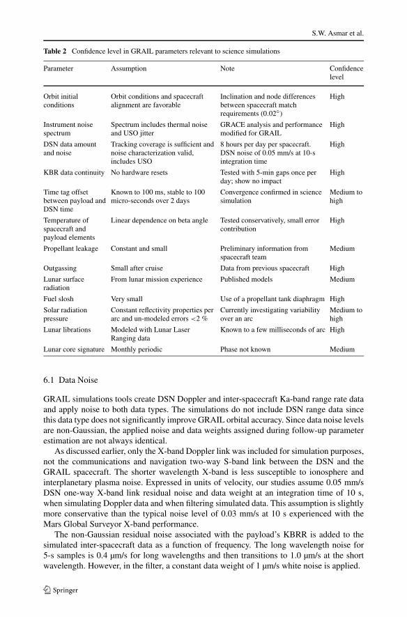
The input parameters to the simulations of the GRAIL mission are discussed below, groupedin the categories of data noise, data coverage, data arcs, orbital parameters, dynamic errors,and kinematic errors. To show the types of issues the simulation team was addressing, Ta-ble 2 lists a summary of parameters relevant to the simulation results and our model confi-dence in each one.

S.W. Asmar et al.

Table 2 Confidence level in GRAIL parameters relevant to science simulations

Parameter Assumption Note Confidencelevel

Orbit initialconditions

Orbit conditions and spacecraftalignment are favorable

Inclination and node differencesbetween spacecraft matchrequirements (0.02◦)

High

Instrument noisespectrum

Spectrum includes thermal noiseand USO jitter

GRACE analysis and performancemodified for GRAIL

High

DSN data amountand noise

Tracking coverage is sufficient andnoise characterization valid,includes USO

8 hours per day per spacecraft.DSN noise of 0.05 mm/s at 10-sintegration time

High

KBR data continuity No hardware resets Tested with 5-min gaps once perday; show no impact

High

Time tag offsetbetween payload andDSN time

Known to 100 ms, stable to 100micro-seconds over 2 days

Convergence confirmed in sciencesimulation

Medium tohigh

Temperature ofspacecraft andpayload elements

Linear dependence on beta angle Tested conservatively, small errorcontribution

High

Propellant leakage Constant and small Preliminary information fromspacecraft team

Medium

Outgassing Small after cruise Data from previous spacecraft High

Lunar surfaceradiation

From lunar mission experience Published models Medium

Fuel slosh Very small Use of a propellant tank diaphragm High

Solar radiationpressure

Constant reflectivity properties perarc and un-modeled errors <2 %

Currently investigating variabilityover an arc

Medium tohigh

Lunar librations Modeled with Lunar LaserRanging data

Known to a few milliseconds of arc High

Lunar core signature Monthly periodic Phase not known Medium

6.1 Data Noise

GRAIL simulations tools create DSN Doppler and inter-spacecraft Ka-band range rate dataand apply noise to both data types. The simulations do not include DSN range data sincethis data type does not significantly improve GRAIL orbital accuracy. Since data noise levelsare non-Gaussian, the applied noise and data weights assigned during follow-up parameterestimation are not always identical.

As discussed earlier, only the X-band Doppler link was included for simulation purposes,not the communications and navigation two-way S-band link between the DSN and theGRAIL spacecraft. The shorter wavelength X-band is less susceptible to ionosphere andinterplanetary plasma noise. Expressed in units of velocity, our studies assume 0.05 mm/sDSN one-way X-band link residual noise and data weight at an integration time of 10 s,when simulating Doppler data and when filtering simulated data. This assumption is slightlymore conservative than the typical noise level of 0.03 mm/s at 10 s experienced with theMars Global Surveyor X-band performance.

The non-Gaussian residual noise associated with the payload’s KBRR is added to thesimulated inter-spacecraft data as a function of frequency. The long wavelength noise for5-s samples is 0.4 µm/s for long wavelengths and then transitions to 1.0 µm/s at the shortwavelength. However, in the filter, a constant data weight of 1 µm/s white noise is applied.

The GRAIL Scientific Measurement System

6.2 Data Coverage and Data Arcs

As a baseline, we simulated 8 hours of DSN daily tracking data for each spacecraft, non-overlapping, for a total of 16 hours. This DSN coverage provides information on absoluteorbit for Ebb or Flow and improves long wavelength gravity field solutions, including thelunar core parameters, but contributes minimally to the global and regional science require-ments. The coverage of the KBRR data is assumed to be continuous. Obtaining 16 hours ofDSN coverage per day, every day, for one mission is considered very challenging due to theloading on the DSN but the requirements were accepted since the prime mission duration isrelatively short, on the order of 3 months.

Since successive momentum dumps occur typically two days apart, GRAIL simulationsassume a two-day data arc length, starting from an epoch of 4 March 2012 (actual epoch var-ied). Longer arcs are typically desirable but the momentum dumps are their natural bound-aries.

6.3 Orbital Parameters

During the 82-day Science Phase, the Moon rotates three times underneath the GRAIL orbit.The collection of gravity data over one complete rotation, 27.3 days, is called one mappingcycle. Ebb and Flow are in a common near-polar, near-circular orbit with a mean altitude ofapproximately 55 km during the prime mission. However, as described in Roncoli and Fujii(2010) the periapsis altitude ranges from approximately 16 km to 51 km above a referencelunar sphere. The Ebb-Flow separation distance is designed to slowly vary. For approxi-mately the first half of the mission, they drift apart and their separation distance increasesfrom ∼85 to ∼225 km and then, with only one small orbit trim maneuver, they drift to-wards each other and the distance decreases to ∼65 km near the end of the mission. Theshorter separation distance is optimum for data exploring the local and regional spatial fea-tures while the segment around the maximum separation is optimum for the determinationof the global studies such as the lunar core parameters, which are the Love number and theperiodic signature of degree 2. The separation distances are designed to ensure that there isno degradation of the Ka-band signal due to multipath off the lunar surface and, accordingto Roncoli and Fujii (2010), a shorter spacecraft separation is required because of the lowerspacecraft altitude.

The spacecraft separation contains a drift in order to reduce the resonance effects corre-sponding to the harmonic of the separation distance. Resonance effect degradation occursat harmonic degrees of the form N = 360/(D/30) where D is the spacecraft separation.This corresponds to degrees 54, 108, and 162 for a 200-km separation distance. For a 50-kmseparation, the resonance occurs much later, starting at degree 216.

The spacecraft inclination varies between approximately 88.4 and 89.85 degrees with atwice-per-month periodic signature. The average inclination, approximately 89.1 degrees,is offset from a perfectly polar orbit to improve the determination of low degree harmoniccoefficients, but kept to a minimum to reduce the gap in data coverage at the poles.

The GRAIL science orbital phase is limited in part by a solar beta angle constraint of49 degree imposed by the capability of the electrical power system; the spacecraft cannotgenerate sufficient power from the solar arrays for angles below this constraint. Figure 14of Roncoli and Fujii (2010) illustrates the time history of the solar beta angle as well as therelationship between beta angle and the duration of solar eclipse during the science phase;eclipse durations are a maximum at the beginning and end and no solar eclipses when thesolar beta angle is near 90 degrees near the middle. For the simulations the Sun-angle is

S.W. Asmar et al.

represented after Park et al. (2012) with the inclination computed with respect to the lunarpole vector, as:

β = 90◦ − cos−1(eh · rsm) (34)

To separate the non-gravitational signature from gravitational effects, a β angle of 90◦ isoptimal. The spacecraft enters terminator crossing at β ∼ 76◦, and for β-angles less thanthis, modeling non-gravitational forces becomes more difficult, as the perturbations changerapidly due to partial shadowing of the orbit.

6.4 Dynamic Errors

The MIRAGE filter estimates both local parameters that are dependent for each data arcand global parameters that are common to all data arcs. The local dynamic parameters thatare estimated include three dimensionless parameters for the solar pressure model of eachspacecraft, a constant scale factor for the force along the sun-spacecraft direction with anominal value of 1.0 and an a priori uncertainty of 0.10 or 10 % of the solar pressure force,and a scale factor for each off normal directions with a nominal value of 0.0 and an a prioriuncertainty of 0.02 or 2 % of the overall solar pressure force. The solar pressure is modeledas a box-wing plate model with appropriate specular and diffuse coefficient values for eachplate. Since both spacecraft are nearly identical, the solutions for the solar pressure scalefactors are expected to be nearly equal. Several gravity solutions were also generated withstrong a priori correlations between the two spacecraft solar pressure solutions to force themto be nearly equal. This constraint improved the core parameter uncertainties by about 30 %but had little effect on the global and regional gravity requirements. The baseline approach,however, is to treat the solar pressure solution of each spacecraft independently.

To account for un-modeled residual solar pressure errors, 15 periodic coefficients areestimated for each spacecraft for each arc with a priori amplitude equal to ∼2 % of the solarpressure force, or 3 × 10−12 km/s2. The coefficients include constant, once per revolutionand twice per revolution amplitudes for the radial, orbit normal, and along the velocitydirections.

The lunar albedo model is not part of the baseline simulations results but albedo errorswere independently investigated and found to be minimal. The albedo surface representationis given by the 10th degree spherical harmonic expansion of Floberhagen et al. (1999).The lunar surface thermal re-radiation is also investigated and is similar in size to albedo.Another non-gravitational force to be considered for GRAIL is the thermal radiation forceas a result of heating on the spacecraft; this force is assumed to be small.

In the estimation of the gravity field, we assume a nominal gravity field and a truth gravityfield. For the early simulation, the lunar gravity model derived from the Lunar Prospectormission to degree and order 150 and designated LP150Q in Konopliv et al. (2001) was usedas both the nominal and truth models. Simulations since then have also used the smallerLP100J lunar gravity model to degree 100 as the nominal model to test convergence to theLP150Q truth model for different modeling assumptions.

The global dynamic parameters that are estimated include a gravity field to a given de-gree, the second-degree Love numbers, and the periodic amplitudes of C21 and S21 for coredetection. In order to reduce computation time, the globally estimated gravity field was todegree 150 and extrapolated the results to degree 180. With current assumptions about dataquality, it is expected that the gravity field will be recovered to higher than degree and order300, which would make the Moon the body with the highest known gravity resolution in theuniverse.

The GRAIL Scientific Measurement System

6.5 Kinematic Errors

In addition to dynamic errors, which directly affect the spacecraft orbit because of a force,there are kinematic errors that affect the KBRR or DSN Doppler observables directly. Mostof the kinematic corrections are estimated as local parameters that affect only that data arc.For every GRAIL orbit period of ∼2 hours, a KBRR bias, drift, and cosine and sine onceper revolution amplitudes are estimated. For a 2-day arc this amounts to 48 parametersbeing estimated. No a priori constraint is applied to these parameters. For each arc, oneDSN Doppler bias and one drift parameter are estimated to correct the USO frequency forthe X-band one-way Doppler.

The very important kinematic error of timing offsets is addressed in a separate sectionbelow. Other kinematic errors are investigated by introducing noise or systematic trends inthe KBRR residuals. The KBRR noise spectrum includes error contributions from the USOand spacecraft attitude jitter and the simulation account for them with a spectrum rangingfrom 0.4 µm/s at the long-wave-length to 1 µm/s at the short wavelength. Errors due to theoffset of the phase center from the line connecting the center-of-mass from each spacecraftare minimized by actively pointing the spacecraft to align the phase centers. The changes inthe temperature of the payload antenna and related hardware are modeled as a systematictrend in the observables. The current models we have investigated are sinusoidal once perorbit tones of 80 µm, a twice per orbit tone, and a triangular shaped twice per orbit signature.Amplitudes of all of these depend on the Sun angle. There is also a small error due to a shiftreactive to the Ka-band system. These errors have a small effect on the core parameters anda negligible effect on the global and regional requirements. Errors due to sloshing of the fuelin the spacecraft fuel tank are expected to be negligible.

7 Modeling System Contributions

GRAIL utilized an integrated scientific measurement system comprised of flight, ground,mission, and data system elements in order to meet the end-to-end performance requiredfor achieving the scientific objectives. Simulations leading to end-to-end error budgets wereused to optimize the design, implementation, and testing of these elements. Because theinter-spacecraft range and range-rate observables and the range-rate between each spacecraftand ground stations can be affected by the performance of all elements of the mission, theywere all treated as parts of an extended science instrument or a science system.

7.1 Flight System

The flight system is the spacecraft, which is comprised of the orbiters and science payload.The orbiter is comprised of the spacecraft bus, heritage from the Experimental SatelliteSystem 11 (XSS-11) mission, and subsystems described in Hoffman (2009). At the heart ofthe flight system is the LGRS payload. Its design and performance are detailed in Klipsteinet al. (2013, this issue). Key components of the GRAIL payload, such as the USO and RSB,are discussed here in the context of the quality of radio links, Doppler data, timing effects,and end-to-end error budgets.

As discussed above, to assess the ability of the flight system to meet the science require-ments, all known sources of dynamic and kinematic error were assessed for their possiblecontributions to the uncertainty of simulated solutions for the gravity field and time vary-ing tidal and core parameters. Fahnestock et al. (2012) described how early calculations

S.W. Asmar et al.

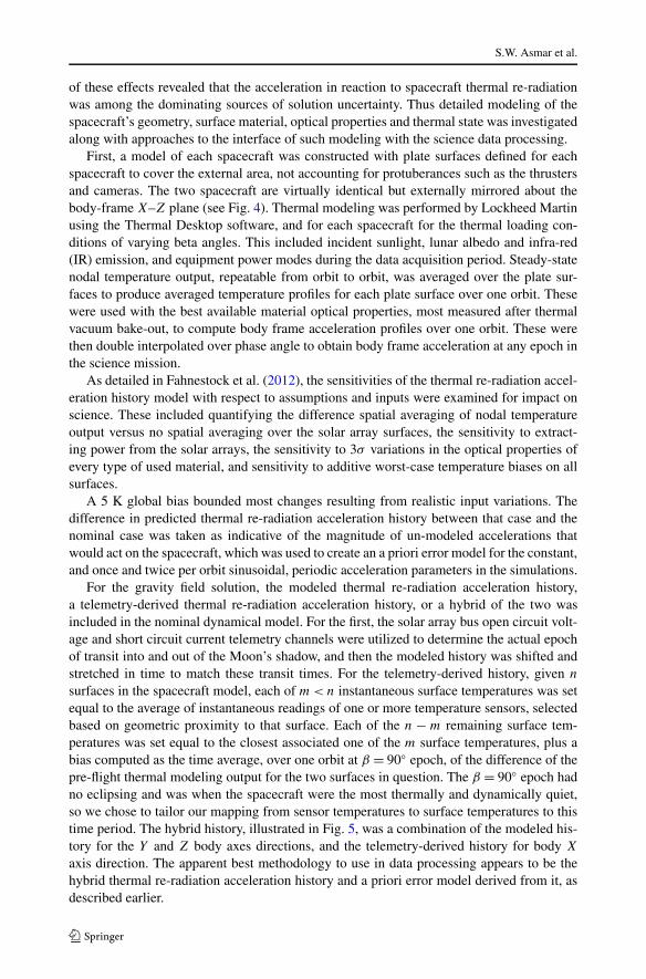
of these effects revealed that the acceleration in reaction to spacecraft thermal re-radiationwas among the dominating sources of solution uncertainty. Thus detailed modeling of thespacecraft’s geometry, surface material, optical properties and thermal state was investigatedalong with approaches to the interface of such modeling with the science data processing.

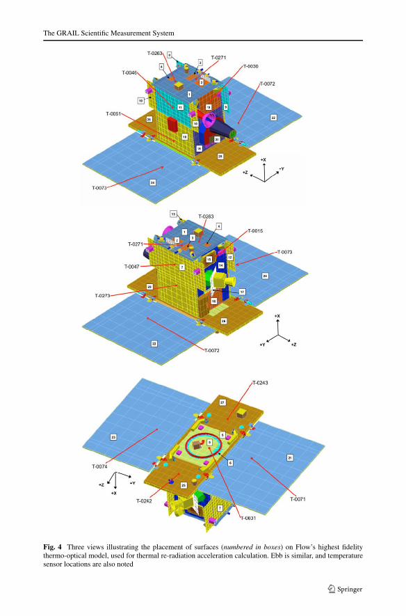
First, a model of each spacecraft was constructed with plate surfaces defined for eachspacecraft to cover the external area, not accounting for protuberances such as the thrustersand cameras. The two spacecraft are virtually identical but externally mirrored about thebody-frame X–Z plane (see Fig. 4). Thermal modeling was performed by Lockheed Martinusing the Thermal Desktop software, and for each spacecraft for the thermal loading con-ditions of varying beta angles. This included incident sunlight, lunar albedo and infra-red(IR) emission, and equipment power modes during the data acquisition period. Steady-statenodal temperature output, repeatable from orbit to orbit, was averaged over the plate sur-faces to produce averaged temperature profiles for each plate surface over one orbit. Thesewere used with the best available material optical properties, most measured after thermalvacuum bake-out, to compute body frame acceleration profiles over one orbit. These werethen double interpolated over phase angle to obtain body frame acceleration at any epoch inthe science mission.

As detailed in Fahnestock et al. (2012), the sensitivities of the thermal re-radiation accel-eration history model with respect to assumptions and inputs were examined for impact onscience. These included quantifying the difference spatial averaging of nodal temperatureoutput versus no spatial averaging over the solar array surfaces, the sensitivity to extract-ing power from the solar arrays, the sensitivity to 3σ variations in the optical properties ofevery type of used material, and sensitivity to additive worst-case temperature biases on allsurfaces.

A 5 K global bias bounded most changes resulting from realistic input variations. Thedifference in predicted thermal re-radiation acceleration history between that case and thenominal case was taken as indicative of the magnitude of un-modeled accelerations thatwould act on the spacecraft, which was used to create an a priori error model for the constant,and once and twice per orbit sinusoidal, periodic acceleration parameters in the simulations.

For the gravity field solution, the modeled thermal re-radiation acceleration history,a telemetry-derived thermal re-radiation acceleration history, or a hybrid of the two wasincluded in the nominal dynamical model. For the first, the solar array bus open circuit volt-age and short circuit current telemetry channels were utilized to determine the actual epochof transit into and out of the Moon’s shadow, and then the modeled history was shifted andstretched in time to match these transit times. For the telemetry-derived history, given n

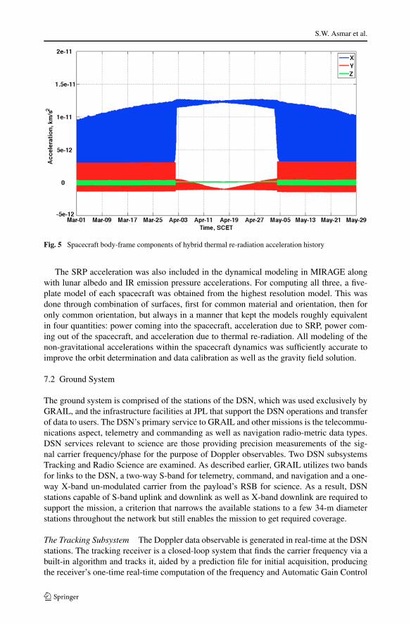
surfaces in the spacecraft model, each of m < n instantaneous surface temperatures was setequal to the average of instantaneous readings of one or more temperature sensors, selectedbased on geometric proximity to that surface. Each of the n − m remaining surface tem-peratures was set equal to the closest associated one of the m surface temperatures, plus abias computed as the time average, over one orbit at β = 90◦ epoch, of the difference of thepre-flight thermal modeling output for the two surfaces in question. The β = 90◦ epoch hadno eclipsing and was when the spacecraft were the most thermally and dynamically quiet,so we chose to tailor our mapping from sensor temperatures to surface temperatures to thistime period. The hybrid history, illustrated in Fig. 5, was a combination of the modeled his-tory for the Y and Z body axes directions, and the telemetry-derived history for body X

axis direction. The apparent best methodology to use in data processing appears to be thehybrid thermal re-radiation acceleration history and a priori error model derived from it, asdescribed earlier.

The GRAIL Scientific Measurement System

Fig. 4 Three views illustrating the placement of surfaces (numbered in boxes) on Flow’s highest fidelitythermo-optical model, used for thermal re-radiation acceleration calculation. Ebb is similar, and temperaturesensor locations are also noted

S.W. Asmar et al.

Fig. 5 Spacecraft body-frame components of hybrid thermal re-radiation acceleration history

The SRP acceleration was also included in the dynamical modeling in MIRAGE alongwith lunar albedo and IR emission pressure accelerations. For computing all three, a five-plate model of each spacecraft was obtained from the highest resolution model. This wasdone through combination of surfaces, first for common material and orientation, then foronly common orientation, but always in a manner that kept the models roughly equivalentin four quantities: power coming into the spacecraft, acceleration due to SRP, power com-ing out of the spacecraft, and acceleration due to thermal re-radiation. All modeling of thenon-gravitational accelerations within the spacecraft dynamics was sufficiently accurate toimprove the orbit determination and data calibration as well as the gravity field solution.

7.2 Ground System

The ground system is comprised of the stations of the DSN, which was used exclusively byGRAIL, and the infrastructure facilities at JPL that support the DSN operations and transferof data to users. The DSN’s primary service to GRAIL and other missions is the telecommu-nications aspect, telemetry and commanding as well as navigation radio-metric data types.DSN services relevant to science are those providing precision measurements of the sig-nal carrier frequency/phase for the purpose of Doppler observables. Two DSN subsystemsTracking and Radio Science are examined. As described earlier, GRAIL utilizes two bandsfor links to the DSN, a two-way S-band for telemetry, command, and navigation and a one-way X-band un-modulated carrier from the payload’s RSB for science. As a result, DSNstations capable of S-band uplink and downlink as well as X-band downlink are required tosupport the mission, a criterion that narrows the available stations to a few 34-m diameterstations throughout the network but still enables the mission to get required coverage.

The Tracking Subsystem The Doppler data observable is generated in real-time at the DSNstations. The tracking receiver is a closed-loop system that finds the carrier frequency via abuilt-in algorithm and tracks it, aided by a prediction file for initial acquisition, producingthe receiver’s one-time real-time computation of the frequency and Automatic Gain Control

The GRAIL Scientific Measurement System

(AGC). Within its design threshold for dynamic conditions and signal-to-noise ratio, theoutput of the receiver is useful with a quantifiable Doppler noise that ranges between 0.02and 0.1 mm/s. For GRAIL simulations, the X-band, USO driven link is associated withDoppler noise of 0.05 mm/s. If the threshold is exceeded, the receiver loses lock and dataare not recoverable.

Radio Science Receiver Designed specifically for Radio Science experiments described inan overview by Asmar (2010), the DSN’s Radio Science Receiver (RSR) is at the heart of anopen-loop reception/recoding subsystem that preserves the raw qualities of the electromag-netic wave propagating from the spacecraft source to the DSN stations. The digital receiverneither locks onto the carrier signal nor makes real-time decisions about its frequency oramplitude. Instead, it down-converts the signal in a predictions-driven heterodyne methodand records the raw complex samples into files for users’ post-pass processing. Asmar et al.(2005) describes the RSR usage and typical performance derived from other missions.

The use of the RSR proved to be critical for enhancing the quantity and quality of GRAILX-band Doppler data in two ways: (1) practically double the amount of RSB data receivedby the DSN by an unofficial use of the concept of multiple-spacecraft per aperture, wherethe DSN station scheduled to track Ebb, for example, also views Flow and vice versa, and(2) contribute to understanding the various timing effects, as explained at length in Sect. 8.GRAIL funded the development of 3 portable RSRs for use throughout the DSN in supportof GRAIL data acquisition and timing synchronization.

7.3 Mission System

The mission operations system is comprised of the JPL and DSN infrastructure as well asthe Lockheed Martin operations. Since the mission design affects science data quality, thefollowing factors had to be very carefully considered: spacecraft altitude and spatial varia-tion of the altitude, spacecraft separation distance, orbit inclination, ground track separation,mission duration, number of maneuvers, time separation of maneuvers, AMD separation,and amount of ground station coverage. Mission design, navigation, deep space stations,and the ground data system critically contribute to the quality of science data. Specifics ofeach factor were described above and additional details on the mission system can be foundin Roncoli and Fujii (2010), Hatch et al. (2010), Beerer and Havens (2012), and Zuber et al.(2013, this issue).

7.4 Data System

The GRAIL Science Data System (SDS) is comprised of all project hardware and softwaretools that contribute to the quality of the science data. Sine the SDS team is the first team toassess the quality of the data on a daily basis, it provides immediate feedback to the MissionSystem on the health of the spacecraft, payload, or ground system in case action is requiredto address an anomaly.

Zuber et al. (2013, this issue) provides a functional block diagram of the SDS that showsthe data flow from all the sources to the final science users and the archives of the PlanetaryData System. For science data processing, delivery, and archiving, the SDS is organizedto provide daily support including weekends in order to handle the data volume as well asprevent any oversight of anomalies for any extended period of time.

S.W. Asmar et al.

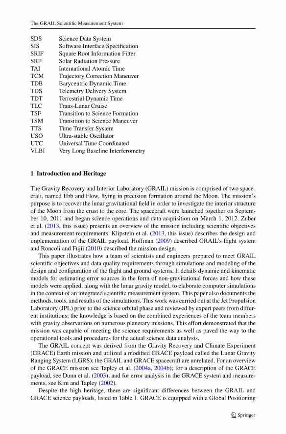
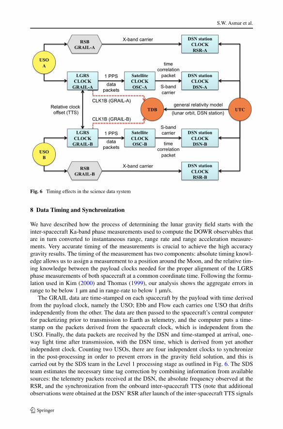
Fig. 6 Timing effects in the science data system

8 Data Timing and Synchronization

We have described how the process of determining the lunar gravity field starts with theinter-spacecraft Ka-band phase measurements used to compute the DOWR observables thatare in turn converted to instantaneous range, range rate and range acceleration measure-ments. Very accurate timing of the measurements is crucial to achieve the high accuracygravity results. The timing of the measurement has two components: absolute timing knowl-edge allows us to assign a measurement to a position around the Moon, and the relative tim-ing knowledge between the payload clocks needed for the proper alignment of the LGRSphase measurements of both spacecraft at a common coordinate time. Following the formu-lation used in Kim (2000) and Thomas (1999), our analysis shows the aggregate errors inrange to be below 1 µm and in range-rate to below 1 µm/s.

The GRAIL data are time-stamped on each spacecraft by the payload with time derivedfrom the payload clock, namely the USO; Ebb and Flow each carries one USO that driftsindependently from the other. The data are then passed to the spacecraft’s central computerfor packetizing prior to transmission to Earth as telemetry, and the computer puts a time-stamp on the packets derived from the spacecraft clock, which is independent from theUSO. Finally, the data packets are received by the DSN and time-stamped at arrival, one-way light time after transmission, with the DSN time, which is derived from yet anotherindependent clock. Counting two USOs, there are four independent clocks to synchronizein the post-processing in order to prevent errors in the gravity field solution, and this iscarried out by the SDS team in the Level 1 processing stage as outlined in Fig. 6. The SDSteam estimates the necessary time tag correction by combining information from availablesources: the telemetry packets received at the DSN, the absolute frequency observed at theRSR, and the synchronization from the onboard inter-spacecraft TTS (note that additionalobservations were obtained at the DSN’ RSR after launch of the inter-spacecraft TTS signals

The GRAIL Scientific Measurement System

edge to deduce the absolute time on-board and correlate it to the known USO drift resultingin micro-second level of accuracy, orders of magnitude better than time correlation packetinformation).

For the purpose of the simulations, it is assumed that the a priori clock offset knowledgeis 100 milliseconds, constant over one month, and that the reconstruction of the time tagoffset is ∼20 microseconds. To achieve such accuracies, the RSB was added to the sciencepayload to transmit a one-way X-band un-modulated sine-wave signal generated by the USOand recorded by the DSN’s RSR. The RSR measurement of the frequency bias is <10−5 Hzand standard deviation = 10−3 Hz.

The DSN clocks are synchronized with the highly stable Coordinated Universal Time(UTC) standard. GRAIL’s data processing, on the other hand, utilizes Barycentric Dynam-ical Time (TDB). The timing analysis derives a time correlation between the LGRS clocksand the TDB time scale, to be provided as a Level 1 ancillary data product called CLK1B.To produce CLK1B relating LGRS and TDB, we preprocess the timing data types and runthem through a non-causal Kalman filter.

The LGRS clock on each spacecraft is driven by the USO for maximum stability, whichis 3 × 10−13 over integration times of 1 to 100 seconds, expressed in Allan Deviation. Thisclock, however, does not report the absolute time but reports readout with respect to theclock startup epoch with errors from the drift of the USO. Relying on the nearly quadraticbehavior of the onboard clock and an assessment of relativistic contributions, we believethat this system enables determining the relative time on Ebb vs. Flow with a bias < 10−7 sand standard deviation = 9 × 10−11 s.

The Onboard Spacecraft Clock (OSC) is derived from a crystal oscillator with inferiorstability to the USO. The onboard computer tags LGRS timing data packets with OSC time,including the LGRS 1 Pulse Per Second (PPS) packet. Ebb and Flow transmit time corre-lation packets to DSN stations where the arrival time is recorded in UTC, which providesa time correlation between the OSC and UTC. The DSN uses very stable hydrogen maserclocks and time-stamps the arrival of telemetry and tracking data in the UTC frame, whichis tied to the International Atomic Time (TAI) frame. Based on DSN monitoring reports,the real-time timing performance of DSN time-tags is at the microsecond level and post-processing analysis improves the performance to the 10−9 second level.

By combining the LGRS/OSC and OSC/UTC time correlation products, a time correla-tion between LGRS time and UTC can be determined and the OSC clock drops out. BecauseOSC error is under one microsecond over intervals shorter than one second, the stabilitycharacteristics of the OSC do not limit LGRS and UTC correlation accuracy. Consideringpossible unknown timing delays in packet transmission, we expect a measurement bias ofup to 100 milliseconds, and standard deviation of up to 30 milliseconds.

9 Relativistic Effects

Turyshev et al. (2013) has developed a realization of astronomical relativistic referenceframes in the solar system and its application to the GRAIL mission. A model was devel-oped for the necessary space-time coordinate transformations for light time computationsaddressed practical aspects of the implementation and all relevant relativistic coordinatetransformations needed to describe the motion of the GRAIL spacecraft and to compute ob-servable quantities. Relativistic effects contributing to the double one-way range observable,which is derived from one-way signal travel times between the two GRAIL spacecraft wereaccounted for and a general relativistic model for this fundamental observable of GRAIL,

S.W. Asmar et al.

accurate to 1 µm and range-rate to 1 µm/s were also developed. The formulation justifiesthe basic assumptions behind the design of the GRAIL mission and may also be used inpost-processing to further improve the results after the mission is complete.

It was recognized early during GRAIL’s development phase that due to the expected highaccuracy of ranging data, models of its observables must be formulated within the frame-work of Einstein’s general theory of relativity in order to avoid significant model discrep-ancy. The ultimate observable model must correctly describe all the timing events occurringduring the science operations of the mission for the links to Earth as well as the inter-spacecraft links. The model must take into account the different times at which the eventshave to be computed, involving the time of transmission of the Ka-band signal at one of thespacecraft, say Ebb, at the reception of this signal by its twin, Flow. In addition, the modelmust include a description of the process of transmitting S-band and X-band signals fromboth spacecraft and reception of this signal at a DSN tracking station.

Relevant points regarding relativistic corrections at the level of accuracy required byGRAIL include: (1) for a spacecraft around the Moon, we can model proper time treatingthe Moon as a point mass; (2) JPL’s long-standing ODP models designed for proper timeof a station on Earth are already sufficiently accurate, with no changes required; (3) up toa constant bias, computing one-way range from DOWR requires a pair of corrections fromone-way light time to instantaneous distance. It suffices to iteratively solve for light time interms of instantaneous distance, by re-computing transmission position bearing in mind theelapsed light time, in the presence of the Shapiro delay.

Turyshev et al. (2013) also notes that measuring the signal frequency involves computingthree numbers: the derivative of proper time at the receiver with respect to coordinate timeof reception, the derivative of proper time at the transmitter with respect to coordinate timeof transmission, and the derivative of coordinate time of reception with respect to coordinatetime of transmission. The first number must be modified to account for the fact that the clockat the DSN receiver attempts to synchronize with UTC time, rather than simply acting as aTDB receiver placed on the surface of the earth. The effect of the Earth’s and the Moon’sgravity on the third term will be below our level of error; if we did choose to include themit would certainly suffice to use a point mass.

10 Results of Simulations

10.1 A Priori Assumptions and Kaula Constraints

The a priori uncertainties for the models used in the simulations are summarized in Table 3.Furthermore, we assume that the KBRR data have σs = 1 µm/s uncertainty at 5-second counttime, and the DSN Doppler tracking uncertainty at 10-second count time σd = 0.05 mm/s,obtained from previous payload and flight experience. The KBRR data give an averageaccuracy of 2×10−10 km/s2, which is equivalent to 0.002 mGal in the gravity measurement.

Gravity field estimates often require a constraint by the Kaula rule (Kaula 1966). In thisstudy, we assume the Kaula constraint to be 2.5 × 10−4/n2. Note that the Kaula constraintapproximates the root-mean-square (RMS) of the spherical harmonics coefficients, i.e.,

RMSn =√

σ 2n

2n + 1, (35)

for the degree variance σ 2n = ∑n

m=0(C2nm + S

2nm).

The GRAIL Scientific Measurement System

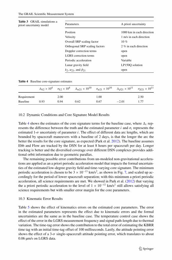
Table 3 GRAIL simulations apriori uncertainty model Parameters A priori uncertainty

Position 1000 km in each direction

Velocity 1 m/s in each direction

Overall SRP scaling factor 10 %

Orthogonal SRP scaling factors 2 % in each direction

Doppler correction terms open

LGRS correction terms open

Periodic acceleration Variable

Lunar gravity field LP150Q solution

k2, α21, and β21 open

Table 4 Baseline core-signature estimates

�k2 × 104 σk2 × 104 �α21 × 1010 σα21 × 1010 �β21 × 1011 σβ21 × 1011

Requirement 2.00 1.00 2.50

Baseline 0.93 0.94 0.62 0.67 −2.01 1.77

10.2 Dynamic Conditions and Core Signature Model Results

Table 4 shows the estimates of the core signature terms for the baseline case, where �i rep-resents the difference between the truth and the estimated parameter i and σi represents theestimated 1-σ uncertainty of parameter i. The effect of different data arc lengths, which arebounded by spacecraft maneuvers with a baseline of 2 days, is that the longer the arc thebetter the results for the core signature, as expected (Park et al. 2012). The baseline assumesEbb and Flow are tracked by the DSN for at least 8 hours per spacecraft per day. Longertracking is better and the diversified coverage over different DSN complexes provides addi-tional orbit information due to geometric parallax.

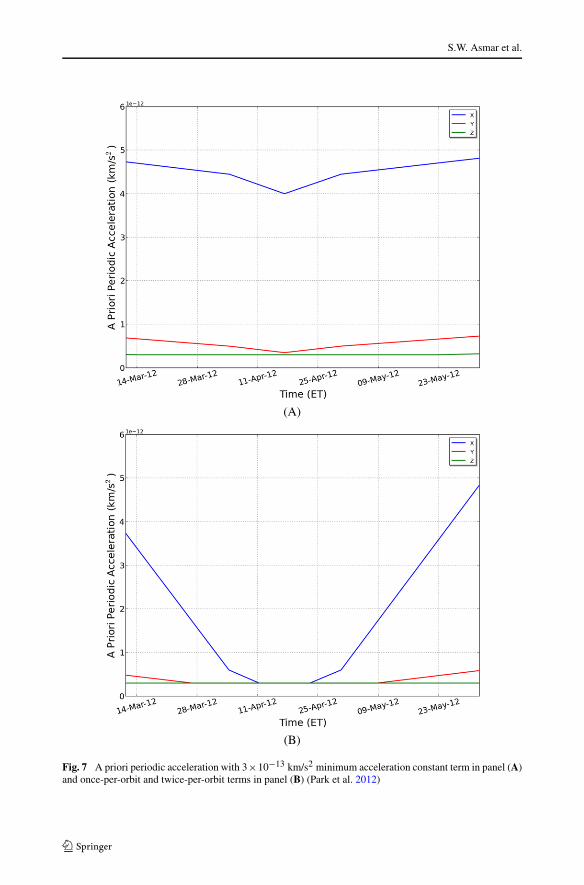
The remaining possible error contributions from un-modeled non-gravitational accelera-tions are applied as an a priori periodic acceleration model that impacts the formal uncertain-ties of the estimated low-degree gravity field and time-varying core signature. The minimumperiodic acceleration is chosen to be 3 × 10−13 km/s2, as shown in Fig. 7, and scaled up ac-cordingly for the period of lower spacecraft separation; with this minimum a priori periodicacceleration, all science requirements are met. We showed in Park et al. (2012) that varyingthe a priori periodic acceleration to the level of 1 × 10−12 km/s2 still allows satisfying allscience requirements but with smaller error margin for the core parameters.

10.3 Kinematic Error Results

Table 5 shows the effect of kinematics errors on the estimated core parameters. The errorin the estimated parameters represents the effect due to kinematic errors and the formaluncertainties are the same as in the baseline case. The temperature control case shows theeffect of the error in the LGRS measurement frequency and signal path-length due to thermalvariation. The time-tag error shows the contribution to the total error of estimating the KBRRtime tag with an initial time-tag offset of 100 milliseconds. Lastly, the attitude pointing errorshows the effect of a 3-σ single-spacecraft attitude pointing error, which translates to about0.06 µm/s on LGRS data.

S.W. Asmar et al.

(A)

(B)

Fig. 7 A priori periodic acceleration with 3×10−13 km/s2 minimum acceleration constant term in panel (A)and once-per-orbit and twice-per-orbit terms in panel (B) (Park et al. 2012)

The GRAIL Scientific Measurement System

Table 5 Effect of kinematicserrors on estimated coreparameters

Cases �k2 × 104 �α21 × 1010

Temperature control 0.05 0.01

Time-tag error 0.02 0.02

Attitude pointing error 0.20 0.10

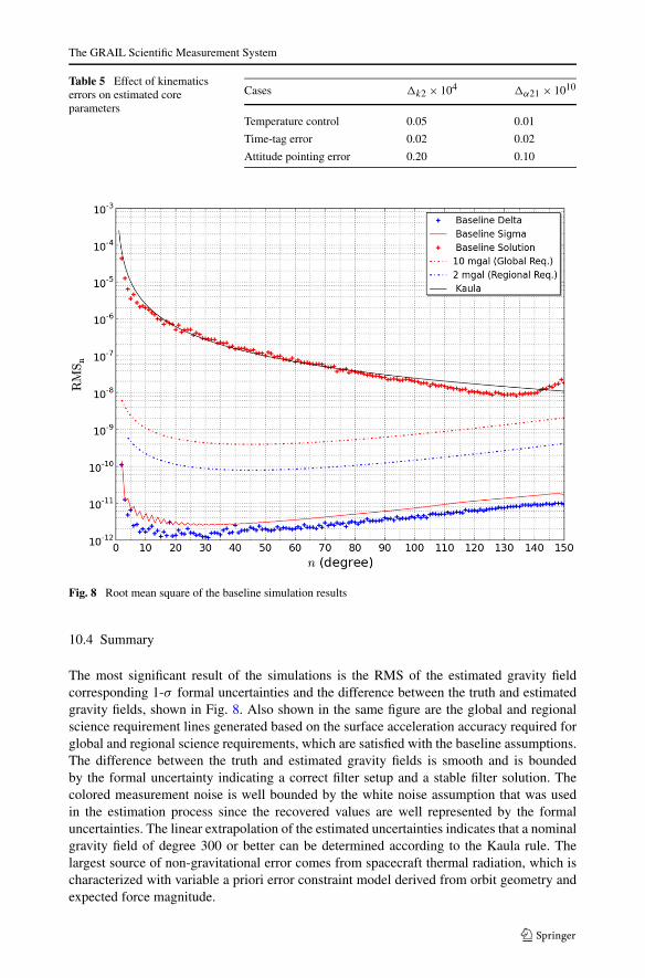
Fig. 8 Root mean square of the baseline simulation results

10.4 Summary

The most significant result of the simulations is the RMS of the estimated gravity fieldcorresponding 1-σ formal uncertainties and the difference between the truth and estimatedgravity fields, shown in Fig. 8. Also shown in the same figure are the global and regionalscience requirement lines generated based on the surface acceleration accuracy required forglobal and regional science requirements, which are satisfied with the baseline assumptions.The difference between the truth and estimated gravity fields is smooth and is boundedby the formal uncertainty indicating a correct filter setup and a stable filter solution. Thecolored measurement noise is well bounded by the white noise assumption that was usedin the estimation process since the recovered values are well represented by the formaluncertainties. The linear extrapolation of the estimated uncertainties indicates that a nominalgravity field of degree 300 or better can be determined according to the Kaula rule. Thelargest source of non-gravitational error comes from spacecraft thermal radiation, which ischaracterized with variable a priori error constraint model derived from orbit geometry andexpected force magnitude.

S.W. Asmar et al.

With all error models included, detailed and numerous simulations show that estimatingthe lunar gravity field is robust against dynamic and kinematic errors and meets the highaccuracy lunar gravity requirements by at least an order of magnitude. A nominal lunargravity field of degree 300 or better can be achieved according to the scaled Kaula rulefor the Moon. The core signature is more sensitive to modeling errors and depends on howaccurately the spacecraft dynamics can be modeled; the requirement can be achieved with asmall margin.

Acknowledgements The GRAIL mission is supported by the NASA Discovery Program under contractsto the Massachusetts Institute of Technology and the Jet Propulsion Laboratory. The work described in thispaper was mostly carried out at Jet Propulsion Laboratory, California Institute of Technology, under contractwith the National Aeronautics and Space Administration. The authors thank colleagues who have contributedto this work or reviewed it, especially at JPL: Duncan McPherson, Ralph Roncoli, William Folkner, KevinBarltrop, Charles Dunn, William Klipstein, Randy Dodge, William Bertch, Daniel Klein, Dong Shin, StefanEsterhausin, Slava Turyshev, Tom Hoffman, Charles Bell, Hoppy Price, Neil Dahya, Joseph Beerer, GlenHavens, Robert Gounley, Ruth Fragoso, Susan Kurtik, Behzad Raofi, and Dolan Highsmith. From LockheedMartin Space Systems Company (Denver): Stu Spath, Tim Linn, Ryan Olds, Dave Eckart, and Brad Haack,Kevin Johnson, Carey Parish, Chris May, Rob Chambers, Kristian Waldorff, Josh Wood, Piet Kallemeyn,Angus McMechan, Cavan Cuddy, and Steve Odiorne. From the NASA Goddard Space Flight Center: FrankLemoine and David Rowlands, and from the University of Texas: Byron Tapley and Srinivas Bettadpur.

References

S. Aoki, H. Kinoshita, Note on the relation between the equinox and Guinot’s non-rotating origin. Celest.Mech. 29, 335–360 (1983)

S. Aoki, B. Guinot, G.K. Kaplan, H. Kinoshita, D. McCarthy, P.K. Seidelmann, The new definition of univer-sal time. Astron. Astrophys. 105, 359–361 (1982)

D.F. Argus, R.G. Gordon, No-net-rotation model of current plate velocities incorporating plate motion modelNUVEL-1. Geophys. Res. Lett. 18, 2039–2042 (1991)

S.W. Asmar, Radio as a science tool. Proc. IEEE 98, 10 (2010)S.W. Asmar, J.W. Armstrong, L. Iess, P. Tortora, Spacecraft Doppler tracking: noise budget and achievable

accuracy in precision radio science observations. Radio Sci. 40 (2005). doi:10.1029/2004RS003101J.G. Beerer, G.G. Havens, Operation the dual-orbiter GRAIL mission to measure the Moon’s gravity, in

SpaceOps 2012 Conference, Stockholm, Sweden, June 2012C. Boucher, Z. Altamimi, L. Duhem, Results and analysis of the ITRF93. IERS Technical Note, 18, Obser-

vatoire de Paris, 1994C. Dunn, W. Bertiger, Y. Bar-Sever, S. Desai, B. Haines, D. Kuang, G. Franklin, I. Harris, G. Kruizinga,

T. Meehan, S. Nandi, D. Nguyen, T. Rogstad, J.B. Thomas, J. Tien, L. Romans, M. Watkins, S.C. Wu,S. Bettadpur, J. Kim, Instrument of GRACE: GPS augments gravity measurements. GPS World 14,16–28 (2003)

E.G. Fahnestock, Comprehensive gravity and dynamics model determination of binary asteroid systems, inAmerican Astronomical Society, DPS Meeting 41, #50.11 (2009)

E.G. Fahnestock, R.S. Park, D.-N. Yuan, A.S. Konopliv, Spacecraft thermal and optical modeling impactson estimation of the GRAIL lunar gravity field, in AIAA/AAS Astrodynamics Specialist Conference,Minneapolis, MN, AIAA, August 13–16, 2012, pp. 2012–4428

R. Floberhagen, P. Visser, F. Weischede, Lunar albedo forces modeling and its effect on low lunar orbit andgravity field determination. Adv. Space Res. 23, 378–733 (1999)

W.M. Folkner, DSN station locations and uncertainties. JPL TDA Progress Report, 42-128, 1-34, Jet Propul-sion Laboratory, California Institute of Technology, Pasadena, CA, 1996

W.M. Folkner, J.A. Steppe, S.H. Oliveau, Earth orientation parameter file description and usage. Interof-fice Memorandum 335.1-11-93 (internal document), Jet Propulsion Laboratory, California Institute ofTechnology, Pasadena, CA, 1993

J. Guinn, P. Wolff, TOPEX/Poseidon operational orbit determination results using global positioning satel-lites, in AAS/AIAA Astrodynamics Specialists Conference (1993). AAS-93-573

S. Hatch, R. Roncoli, T. Sweetser, GRAIL trajectory design: lunar orbit insertion through science, in AIAAGuidance, Navigation, and Control Conference, Toronto, Ontario, Canada, August 2010. AIAA 2010-8385

The GRAIL Scientific Measurement System

W.A. Heiskanen, H. Moritz, Physical geodesy. Bull. Géod. 86(1), 491–492 (1967)T.L. Hoffman, GRAIL: gravity mapping the Moon, in Aerospace Conference, 2009 IEEE, Big Sky, MT, 7–14

March 2009. ISBN 978-1-4244-2622-5W.M. Kaula, Theory of Satellite Geodesy (Blaisdell, Waltham, 1966). 124 pp.J. Kim, Simulation study of a low-low satellite-to-satellite tracking mission. Ph.D. dissertation, Univ. of Texas

at Austin, May 2000J. Kim, B. Tapley, Error analysis of a low-low satellite-to-satellite tracking mission. J. Guid. Control Dyn.

25(6), 1100–1106 (2002)W.M. Klipstein, B.W. Arnold, D.G. Enzer, A.A. Ruiz, J.Y. Yien, R.T. Wang, C.E. Dunn, The lunar gravity

ranging system for the gravity recovery and interior laboratory (GRAIL) mission. Space Sci. Rev. (2013,this issue)

A.S. Konopliv, S.W. Asmar, E. Carranza, D.N. Yuan, W.L. Sjogren, Recent gravity models as a result of thelunar prospector mission. Icarus 150, 1–18 (2001)

F.T. Krogh, Changing stepsize in the integration of differential equations using modified divided differences.JPL Tech. Mem. No. 312, Section 914 (internal document), Jet Propulsion Laboratory, California Insti-tute of Technology, Pasadena, CA, 1973

C.L. Lawson, R.J. Hanson, Solving Least Squares Problems. SIAM Classics in Applied Mathematics, vol. 15(Society for Industrial and Applied Mathematics, Philadelphia, 1995)

R. Leavitt, A. Salama, Design and implementation of software algorithms for TOPEX/POSEIDON ephemerisrepresentation, in AIAA/AAS Astrodynamics Specialists Conference (1993). AAS-93-724

J.H. Lieske, T. Lederle, W. Fricke, B. Morando, Expressions for the precession quantities based upon the IAU(1976) system of astronomical constants. Astron. Astrophys. 58, 1–16 (1977)

A.J. Mannucci, B.D. Wilson, D.-N. Yuan, C.H. Ho, U.J. Lindqwister, T.F. Runge, A global mapping techniquefor GPS-derived ionospheric total electron content measurements. Radio Sci. 33(3), 565–582 (1998)

D.D. McCarthy, G. Petit (eds.), IERS Conventions, IERS Technical Note, vol. 32 (2003)T.D. Moyer, Formulation for Observed and Computed Values of Deep Space Network Data Types for Navi-

gation (Wiley, Hoboken, 2003). 576 pp.X.X. Newhall, J.G. Williams, Estimation of the lunar physical librations. Celest. Mech. Dyn. Astron. 66,

21–30 (1997)R.S. Park, S.W. Asmar, E.G. Fahnestock, A.S. Konopliv, W. Lu, M.M. Watkins, Gravity recovery and interior

laboratory simulations of static and temporal gravity field. J. Spacecr. Rockets 49, 390–400 (2012)S. Pines, Uniform representation of the gravitational potential and its derivatives. AIAA J. 11, 1508–1511

(1973)R. Roncoli, K. Fujii, Mission design overview for the gravity recovery and interior laboratory (GRAIL)

mission, in AIAA Guidance, Navigation, and Control Conference, Toronto, Ontario, Canada, August2010. AIAA 2010-8383

P.K. Seidelmann, 1980 IAU theory of nutation: the final report of the IAU working group on nutation. Celest.Mech. 27, 79–106 (1982)

B.D. Tapley, B. Schutz, G. Born, Statistical Orbit Determination (Elsevier, Boston, 2004a). 547 pp.B.D. Tapley, S. Bettadpur, M. Watkins, C. Reigber, The gravity recovery and climate experiment: mission

overview and early results. Geophys. Res. Lett. 31 (2004b). doi:10.1029/2004GL019920B.J. Thomas, An analysis of gravity-field estimation based on intersatellite dual-1-way biased ranging. JPL

Publication 98–15, May 1999S.G. Turyshev, V.T. Toth, M.V. Sazhin, General relativistic observables of the GRAIL mission. Phys. Rev. D

87, 024020 (2013)J.M. Wahr, The forced nutations of an elliptical, rotating, elastic, and oceanless Earth. Geophys. J. R. Astron.

Soc. 64, 705–727 (1981)R.C. Weber, P.-Y. Lin, E.J. Garnero, Q. Williams, P. Lognonne, Seismic detection of the lunar core. Science

331, 309–313 (2011). doi:10.1126/science.1199375J.G. Williams, A scheme for lunar inner core detection. Geophys. Res. Lett. 34, L03202 (2007).

doi:10.1029/2006GL028185J.G. Williams, D.H. Boggs, W.M. Folkner, DE421 lunar orbit, physical librations, and surface coordinates.

JPL IOM 335-JW, DB, WF-20080314-001, March 14, 2008D.-N. Yuan, W. Sjogren, A. Konopliv, A. Kucinskas, Gravity field of mars: a 75th degree and order model.

J. Geophys. Res. 106(E10), 23377–23401 (2001)M.T. Zuber, D.E. Smith, D.H. Lehman, T.L. Hoffman, S.W. Asmar, M.M. Watkins, Gravity recovery and

interior laboratory (GRAIL): mapping the lunar interior from crust to core. Space Sci. Rev. (2013, thisissue). doi:10.1007/s11214-012-9952-7