9Internal Wavesand Small-ScaleProcesses

Walter Munk

9.1 Introduction

Gravity waves in the ocean's interior are as commonas waves at the sea surface-perhaps even more so, forno one has ever reported an interior calm.

Typical scales for the internal waves are kilometersand hours. Amplitudes are remarkably large, of theorder of 10 meters, and for that reason internal wavesare not difficult to observe; in fact they are hard not toobserve in any kind of systematic measurements con-ducted over the appropriate space-time scales. Theyshow up also where they are not wanted: as short-period fluctuations in the vertical structure of temper-ature and salinity in intermittent hydrocasts.

I believe that Nansen (1902) was the first to reportsuch fluctuations;l they were subsequently observedon major expeditions of the early nineteen hundreds:the Michael Sars expedition in 1910, the Meteor ex-peditions in 1927 and 1938, and the Snellius expeditionin 1929-1930. [A comprehensive account is given inchapter 16 of Defant (1961a)]. In all of these observa-tions the internal waves constitute an undersampledsmall-scale noise that is then "aliased" into the largerspace- time scales that are the principal concern of clas-sical oceanography.

From the very beginning, the fluctuations in the hy-drocast profiles were properly attributed to internalwaves. The earliest theory had preceded the observa-tions by half a century. Stokes (1847) treated internalwaves at the interface between a light fluid overlayinga heavy fluid, a somewhat minor extension of the the-ory of surface waves. The important extension to thecase of a vertical mode structure in continuously strat-ified fluids goes back to Rayleigh (1883). But the dis-creteness in the vertical sampling by hydrocasts led toan interpretation in terms of just the few gravestmodes, with the number of such modes increasing withthe number of sample depths (giving j equations in junknowns). And the discreteness in sampling time ledto an interpretation in terms of just a few discretefrequencies, with emphasis on tidal frequencies.

The development of the bathythermograph in 1940made it possible to repeat soundings at close intervals.Ufford (1947) employed three vessels from which bath-ythermograph lowerings were made at 2-minute inter-vals! In 1954, Stommel commenced three years of tem-perature observations offshore from Castle Harbor,Bermuda, initially at half-hour intervals, later at 5-min-ute intervals. 2 Starting in 1959, time series of isothermdepths were obtained at the Navy Electronics Labora-tory (NEL) oceanographic tower off Mission Beach, Cal-ifornia, using isotherm followers (Lafond, 1961) in-stalled in a 200-m triangle (Cox, 1962).

By this time oceanographers had become familiarwith the concepts of continuous spectra (long before

264Walter Munk

�II_____I____�_ _ _ _

routinely applied in the fields of optics and acoustics),and the spectral representation of surface waves hadproven very useful. It became clear that internal waves,too, occupy a frequency continuum, over some six oc-taves extending from inertial to buoyant frequencies.[The high-frequency cutoff had been made explicit byGroen (1948).] With regard to the vertical modes, thereis sufficient energy in the higher modes that for manypurposes the discrete modal structure can be replacedby an equivalent three-dimensional continuum.

We have already referred to the measurements byUfford and by Lafond at horizontally separated points.Simultaneous current measurements at vertically sep-arated points go back to 1930 Ekman and Helland-Hansen, 1931). In all these papers there is an expressionof dismay concerning the lack of resemblance betweenmeasurements at such small spatial separations of os-cillations with such long periods. I believe (from dis-cussions with Ekman in 1949) that this lack of coher-ence was the reason why Ekman postponed for 23 years(until one year before his death) the publication of"Results of a Cruise on Board the 'Armauer Hansen' in1930 under the Leadership of Bjrnm Helland-Hansen"(Ekman, 1953). But the decorrelation distance is justthe reciprocal of the bandwidth; waves separated inwavenumber by more than Ak interfere destructivelyat separations exceeding (Ak)-. The small observedcoherences are simply an indication of a large band-width.

The search for an analytic spectral model to describethe internal current and temperature fluctuations goesback over many years, prompted by the remarkablesuccess of Phillips's (1958) saturation spectrum for sur-face waves. I shall mention only the work of Murphyand Lord (1965), who mounted temperature sensors inan unmanned submarine at great depth. They foundsome evidence for a spectrum depending on scalarwavenumber as k-5'3, which they interpreted as theinertial subrange of homogeneous, isotropic turbu-lence. But the inertial subrange is probably not appli-cable (except perhaps at very small scales), and thefluctuations are certainly not homogeneous and notisotropic.

Briscoe (1975a) has written a very readable accountof developments in the early 1970s. The interpretationof multipoint coherences in terms of bandwidth wasthe key for a model specturm proposed by Garrett andMunk (1972b). The synthesis was purely empirical,apart from being guided by dimensional considerationsand by not violating gross requirements for the finite-ness of certain fundamental physical properties. Sub-sequently, the model served as a convenient "straw-man" for a wide variety of moored, towed and"dropped" experiments, and had to be promptly mod-ified [Garrett and Munk (1975), which became known

as GM75 in the spirit of planned obsolescence]. Therehave been further modifications [see a review paper byGarrett and Munk (1979)]; the most recent version issummarized at the end of this chapter.

The best modem accounts on internal waves are byO. M. Phillips '(1966b), Phillips (1977a), and Turner(1973a). Present views of the time and space scales ofinternal waves are based largely on densely sampledmoored, towed, and dropped measurements. The pi-oneering work with moorings was done at site D in thewestern North Atlantic (Fofonoff, 1969; Webster,1968). Horizontal tows of suspended thermistor chains(Lafond, 1963; Charnock, 1965) were followed by towedand self-propelled isotherm-following "fishes" (Katz,1973; McKean and Ewart, 1974). Techniques fordropped measurements were developed along a numberof lines: rapidly repeated soundings from the stableplatform FLIP by Pinkel (1975), vertical profiling ofcurrents from free-fall instruments by Sanford (1975)and Sanford, Drever, and Dunlap (1978), and verticalprofiling of temperature from a self-contained yo-yoingcapsule by Cairns and Williams (1976). The three-di-mensional IWEX (internal wave experiment) array isthe most ambitious to date (Briscoe, 1975b). These ex-periments have served to determine selected parame-ters of model spectra; none of them so far, not evenIWEX, has been sufficiently complete for a straight-forward and unambiguous transform into the multi-dimensional (co,k)-spectrum. The FLIP measurementscome closest, giving an objective spectrum in the twodimensions o, k, with fragmentary information on ka,k,. Otherwise only one-dimensional spectra can beevaluated from any single experiment, and one is backto model testing. Yet in spite of these observationalshortcomings, there is now evidence for some degreeof universality of internal wave spectra, suggesting thatthese spectra may be shaped by a saturation process(the interior equivalent of whitecaps), rather than byexternal generation processes.

Internal waves have surface manifestations consist-ing of alternate bands of roughened and smooth water(Ewing, 1950; Hughes, 1978), and these appear to bevisible from satellites (figure 9.1). High-frequency sonarbeams are a powerful tool for measuring internal waverelated processes in the upper oceans (figures 9.2, 9.3).The probing of the deep ocean interior by acoustics isultimately limited by scintillations. due to internalwaves (Flatte et al., 1979; Munk and Wunsch, 1979)just as the "diffraction-limited" telescope has its di-mensions set by the small-scale variability in the upperatmosphere.

It will be seen that internal waves are a lively subject.The key is to find the connections between internalwaves and other ocean processes. The discovery of everfiner scales, down to the scale of molecular processes,

265Internal Waves

Figure 9.I SEASAT synthetic aperture radar image off Cabo area. The pattern in the right top area is most likely formedSan Lzaro, Baja California (24°48'N, 112°18'W) taken on 7 by internal waves coming into the 50 fathom line. (I amJuly 1978. Scale of image nearly matches that of bathymetric indebted to R. Bernstein for this figure.)

CT UT23 24 25 23 24

I i1 -_ I 1 I I 1

I I I

(

30 -

Ar'

on

Aet 'C . $'''-ae*

_ ~ ~ ~ ~ : ' 4 __.. '_ ' " '' -e ' ' ' : n,. ; ': 7'

,,-:ta:? , ,) ': ,. 7 : .. ,, .. ~, ."? ;,

0 5 10

Time (min)

Figure 9.2 The water column is insonified with a narrowdownward sonar beam of 200 kHz (wavelength 0.75 cm). Thedark band is presumably a back-scattering layer convolutedby shear instabilities. In a number of places the instabilitieshave created density inversions. This is confirmed by the twoo-t-profiles. The acoustic reflection from the sinking CTDalong the steeply slanting lines shows the depth-time historyof the rr,-profiles. The profiling sound source was suspendedfrom a drifting ship. The horizontal distance between over-turning events was estimated to be 60-70 m. (I am indebtedto Marshall Orr of Woods Hole Oceanographic Institution forthis figure; see Haury, Briscoe, and Orr, 1979.)

266Walter Munk

0

15

Ev:

^s_ __Il_·C

: · � ..

ti,

A h

I

o, ' '_

has been a continuing surprise to the oceanographiccommunity for 40 years. Classical hydrographic castsemployed reversing (Nansen) bottles typically at 100-m intervals in the upper oceans beneath the thermo-cline, and half-kilometer intervals at abyssal depths.Only the gross features can be so resolved. Modemsounding instruments (BT, STD, CTD) demonstrateda temperature and salinity3 fine structure down to me-ter scales. An early clue to microstructure was thesteppy traces on the smoked slides of bathythermo-graphs. These steps were usually attributed to "stylusstiction," and the instruments suitably repaired.

Free-fall apparatus sinking slowly (-0.1 ms-}) andemploying small, rapid-response (-0.01 s) transducers,subsequently resolved the structure down to centime-ter scales and beyond. The evolving terminology

gross structure:fine structure:microstructure:

a,CW

larger than 100 m vertical1 m to 100 m verticalless than 1 m vertical

01 02 03 04

II June 1977 (hr)

is then largely based on what could be resolved in agiven epoch (see chapter 14). The fine-structure meas-urements of temperature and salinity owe much oftheir success to the evolution of the CTD (Brown,1974). The pioneering microscale measurements weredone by Woods (1968a) and by Cox and his collaborators(Gregg and Cox, 1972; Osborn and Cox, 1972). Meas-urements of velocity fine structure down to a few me-ters have been accomplished by Sanford (1975) andSanford, Drever, and Dunlap (1978). Osborn (1974,1980) has resolved the velocity microstructure between40 and 4 cm. Evidently velocity and temperature struc-ture have now been adequately resolved right down tothe scales for which molecular processes become dom-inant. At these scales the dissipation of energy andmean-square temperature gradients is directly propor-tional to the molecular coefficients of viscosity andthermal diffusivity. The dissipation scale for salinityis even smaller (the haline diffusivity is much smallerthan the thermal diffusivity) and has not been ade-quately resolved. The time is drawing near when weshall record the entire fine structure and microstruc-ture scales of temperature, salinity and currents [andhence of the buoyancy frequency N(z) and of Richard-son number Ri(z)] from a single free-fall apparatus.

Perhaps the discovery of very fine scales couldhave been anticipated. There is an overall ocean bal-ance between the generation and dissipation of mean-square gradients. Eckart (1948) refers to the balancingprocesses as stirring and mixing. Garrett (1979) has putit succinctly: "Fluctuations in ocean temperature pro-duced by surface heating and cooling, and in salinitydue to evaporation, precipitation, run-off and freezing,are stirred into the ocean by permanent current sys-tems and large scale eddies." Mixing ultimately occurs

Figure 9.3 Measurements of Doppler vs. range were made at2-minute intervals with a quasi-horizontal 88-kHz soundbeam mounted on FLIP at a depth of 87 m. Bands of alternat-ing positive and negative Doppler in velocity contours) arethe result of back scatter from particles drifting toward andaway from the sound source (the mean drift has been re-moved). The velocities are almost certainly associated withinternal wave-orbital motion. The range-rate of positive ornegative bands gives the appropriate projection of phase ve-locity. The measurements are somewhat equivalent to suc-cessive horizontal tows at 3000 knots! (I am indebted to Rob-ert Pinkel of Scripps Institution of Oceanography for thisfigure.)

through dissipation by "molecular action on small-scale irregularities produced by a variety of processes."The microstructure (where the mean-square gradientslargely reside) are then a vital component of oceandynamics. This leaves open the question whether mix-ing is important throughout the ocean, or whether itis concentrated at ocean boundaries and internal fronts,or in intense currents an extensive discussion may befound in chapter 8).

What are the connections between internal wavesand small-scale ocean structure? Is internal wavebreaking associated with ocean microstructure? Isthere an associated flux of heat and salt, and hencebuoyancy? Does the presence of internal waves in ashear flow lead to an enhanced momentum flux, whichcan be parameterized in the form of an eddy viscosity?What are the processes of internal-wave generation anddecay? I feel that we are close to having these puzzlesfall into place (recognizing that oceanographic "break-throughs" are apt to take a decade), and I am uncom-fortable with attempting a survey at this time.

Forty years ago, internal waves played the role of anattractive nuisance: attractive for their analytical ele-

267Internal Waves

gance and their accessibility to a variety of experimen-tal methods, a nuisance for their interference withwhat was then considered the principal task of physicaloceanography, namely, charting the "mean" densityfield. Twenty years from now I expect that internalwaves will be recognized as being intimately involvedwith the vertical fluxes of heat, salt, and momentum,and so to provide a vital link in the understanding ofthe mean fields of mass and motion in the oceans.

9.1.1 Preview of This ChapterWe start with the traditional case of a two-layer ocean,followed by a discussion of continuous stratification:constant buoyancy frequency N, N decreasing withdepth, a maximum N (thermocline), a double maxi-mum. Conditions are greatly altered in the presence ofquite moderate current shears. Short (compliant) inter-nal waves have phase velocities that are generallyslower than the orbital currents associated with thelong (intrinsic) internal waves, and thus are subject tocritical layer processes. There is further nonlinear cou-pling by various resonant interactions.

Ocean fine structure is usually the result of internal-wave straining, but in some regions the fine structureis dominated by intrusive processes. Microstructure isconcentrated in patches and may be the residue ofinternal wave breaking. Little is known about thebreaking of internal waves. Evidently, there are twolimiting forms of instability leading to breaking: ad-vective instability and shear instability.

The chapter ends with an attempt to estimate theprobability of wave breaking, and of the gross verticalmixing and energy dissipation associated with thesehighly intermittent events. An important fact is thatthe Richardson number associated with the internalwave field is of order 1. Similarly the wave field iswithin a small numerical factor of advective instabil-ity. Doubling the mean internal wave energy can leadto a large increase in the occurrence of breaking events;halving the wave energy could reduce the probabilityof breaking to very low levels. This would have theeffect of maintaining the energy level of internal waveswithin narrow limits, as observed. But the analysis isbased on some questionable assumptions, and the prin-cipal message is that we do not understand the prob-lem.

9.2 Layered Ocean

We start with the conventional discussion of internalwaves at the boundary between two fluids of differentdensity. The configuration has perhaps some applica-tion to the problem of long internal waves in the ther-mocline, and of short internal waves in a stepwise finestructure.

Following Phillips (1977a), this can be treated as alimiting case of a density transition from p, above z =-h to pi beneath z = -h, with a transition thickness8h (figure 9.4). The vertical displacement {(z) has a peakat the transition, and the horizontal velocity u z)changes sign, forming a discontinuity (vortex sheet) inthe limit 8h -O 0. For the second mode (not shown), C(z)changes sign within the transition layer and u(z)changes sign twice; this becomes unphysical in thelimit Ah - 0. For higher modes the discontinuities areeven more pathological, and so a two-layer ocean isassociated with only the gravest internal mode.

For the subsequent discussion it is helpful to give asketch of how the dependent variables are usually de-rived and related. The unknowns are u,v,w,p (aftereliminating the density perturbation), where p is thedeparture from hydrostatic pressure. The four un-knowns are determined by the equations of motion andcontinuity (assuming incompressibility). The linear-ized x,y equations of motion are written in the tradi-tional f-plane; for the vertical equation it is now stan-dard [since the work of Eckart (1960)] to display thedensity stratification in terms of the buoyancy (orBrunt-Vaisala) frequency

(9.1)

thus giving

Ow = 1 P- N 2= 0.

Ot po t

The last term will be recognized as the buoyancy force-g 8ppo of a particle displaced upwards by an amountl = fwdt.

For propagating waves of the form (z) expi(kx - t)the equations can beand §5.7) into

combined (Phillips, 1977a, §5.2

o U- U -'

o o

'l

p N-_Z i

+ ' l 0

iif~

iH

Figure 9.4 A sharp density transition from p, to PI takes placebetween the depths -z = h - 8h and -z = h + 18h. This isassociated with a delta-like peak in buoyancy frequency N(z).Amplitudes of vertical displacement 4(z), horizontal velocityu(z), and shear u'(z) = duldz are sketched for the gravestinternal wave mode.

268Walter Munk

-g['--[~ -(d~jz diabaticl l

d2-- + Nk2 - =o. (9.2)dz2 w 2 -f 2

The linearized boundary conditions are 0 = 0 at thesurface and bottom.

A simple case is that of f = 0 and N = 0 outside thetransition layer. We have then

C. = A sinhkz,

1 = B sinhk(z + H),

above and below the transition layer, respectively. Theconstants A and B are determined by patching the ver-tical displacement at the transition layer:

u = =a at z = -h.

The dispersion relation is found by integrating Eq. (9.2)across the transition layer:

C - 1 = -k24 N(Z) - W2

- 9(g- p - 28h) at z = -h,

transition where N reaches a maximum, but just theopposite is true. To prove this, we use the condition ofincompressibility, iku(z) - io4' = 0, and equation (9.2)to obtain

U = c = N 2z) - kak o~~~~c (9.3)

and so u' - N2 for small wIN; accordingly u'/N variesas N. Thus the layers of largest gravitational stability(largest N) are also the layers of largest shear instability(largest u'/NI).

9.3 Continuously Stratified Ocean

The simplest case is that of constant N. The solutionto (9.2) is

4(z) = a sinmz, m2 = k2N '2 -(a _2 f2 (9.4)

with m so chosen that ; vanishes at z = -H. Solvingfor to2,

where 5' ddz. In the limit of small k h, that is, forwaves long compared to the transition thickness, theforegoing equations lead to the dispersion relation

g(2plp)kcothkh + cothk(H - h)

For a lower layer that is deep as compared to a wave-length, the denominator becomes cothk(h - H) + 1.If the upper layer is also deep, it becomes 1 + 1, and

1 p 1 k P lk P'- P,2 p 2 g(pt + p.)'

As p, - 0, O2 --) gk, which is the familiar expressionfor surface waves in deep water.

The case of principal interest here is that of an iso-lated density transition 8p << p and k 8h << 1. Theno2 = tgk 8pip. The vertical displacement is a maximumat the transition and dies off with distance & from thetransition as a exp( -kl&l).

A question of interest is the variation of Richardsonnumber across the transition layer. We know from thework of Miles and Howard [see Miles (1963)] that fora transition p(z) and a steady u(z) of the kind shown infigure 9.4, the flow becomes unstable to disturbancesof length scale h if Ri < . I find it convenient to referto the root-reciprocal Richardson number

Ri-1 2 = Iu'/NI,

so that large values imply large instabilities (as for Rey-nolds numbers); the critical value is u'/N = 2. Onewould think offhand that u'/N is a minimum at the

2 k2N2 + mjf 2

o= m + k2' mH = jrr,mJ +k

j = 1,2,.... (9.5)

This dispersion relation is plotted in figure 9.5. Thevertical displacements for the first and third mode areshown in figure 9.6. Very high modes (and the oceanis full of them) in the deep interior are many wave-lengths removed from the boundaries, and we can ex-pect the waves to be insensitive to the precise config-uration of top and bottom. The discrete dispersion %w(k)is then replaced by an equivalent continuous dispersionc(k, m).

The standard expressions for the particle velocitiesu,w and the group velocities c with componentsol/Ok, aOwOm as functions of the propagation vector

N

C,

k (cpkm)

Figure 9.5 The dispersion Blwk) [equation (9.5)], for modesj = 1, 10, 100, 1000, corresponding to vertical wavenumbersm = 0.1, 1, 10, 100 cpkm in an ocean of depth 5 km. The in-ertial frequency is taken at f = 0.0417 cph (1 cpd), and thebuoyancy frequency at N = 1 cph.

269Internal Waves

10

N _

U

-z

-H

C (z)

Figure 9.6 Vertical displacements i(z) in a constant-N ocean,for modes = 1 and i = 3.

z

near inertialfrequency

kI>8

x

Cg

znear buoyancyfrequency

i,k

Cg

Figure 9.7 The wavenumber vector k = (k, m) and group ve-locity cg near the inertial frequency to = f + E) and near thebuoyancy frequency {to = N - E}, respectively. A packet ofwave energy is projected on the (x, z)-plane. Crests and troughsin the wave packet are in a plane normal to k, and travel withphase velocity c in the direction k. The wave packet travelswith group velocity cg at right angles to k, thus sliding side-ways along the crests and troughs. The particle velocity u (notshown) is in the planes at right angles to k.

k = (k, m) are easy to derive, but hard to visualize. Con-sider a wave packet (figure 9.7) with crests and troughsalong planes normal to the paper and inclined withrespect to the (x, z)-axis as shown. The phase velocityis in the direction k normal to the crests, but the groupvelocity cg is parallel to the crests, and the wave packetslides sideways. k is inclined to the horizontal by

m (N 2- a1/2tan 8 = = (2_f2 (9.6a)

and so the angle is steep for inertial waves (o = f + E)and flat for buoyancy waves (0o = N - E). The energypacket is propagated horizontally for inertial waves,and vertically for buoyancy waves, but the group ve-locity goes to zero at both limits.

The flow u = (u, w) takes place in the plane of thecrest and troughs. For inertial waves, particles move inhorizontal circles. The orbits become increasingly el-liptical with increasing frequency, and for buoyancywaves the particle orbits are linear along the z-axis, inthe direction of cg. The wavenumber k is always nor-mal to both cg and u. [The nonlinear field accelerations(u V)u vanish for an isolated elementary wave train,leading to the curiosity that the linear solution is anexact solution.] Readers who find it difficult to visu-alize (or believe) these geometric relations should referto the beautiful laboratory demonstrations of Mowbrayand Rarity (1967).

It is not surprising, then, that internal waves will dounexpected things when reflected from sloping bound-aries. The important property is that the inclination 0relative to the x-axis depends only on frequency [equa-tion (9.6a)]. Since frequency is conserved upon reflec-tion, incident and reflected 0 must be symmetric withrespect to a level surface rather than with respect tothe reflecting surface. At the same time the flow u forthe combined incident and reflected wave must be par-allel to the reflecting boundary. For a given co, there isa special angle for which the orbital flow is parallel tothe boundary. This requires that the boundary be in-clined at a slope

tan/i(z) = tan(900- =0) =[:z - L2] (9.6b)

It can be shown that for slopes steeper than /, theenergy of "shoreward" traveling internal waves is re-flected "seaward": for slopes of less than /3, the energyis forward reflected. Repeated reflections in a wedge-shaped region such as the ocean on the continentalslope can lead to an accumulation of energy at eversmaller scales (Wunsch, 1969). For a given slope, wecan expect an amplification of the internal waves atthe frequency co determined by (9.6b). Wunsch (1972b)has suggested that a peak in the spectrum of temper-ature fluctuations measured southeast of Bermuda

270Walter Munk

! i 1�

o0l

could be so explained. Pertinent values are N =

2.6 cph, f = 0.045 cph, and i- 13°. Equation (9.6b)gives o = 0.59 cph, in agreement with the observedspectral peak at 0.5 cph.

9.4 Turning Depths and Turning Latitudes

Figure 9.8 shows the situation for an ocean with vari-able N(z). For frequencies that are less than N through-out the water column, the displacements are similar tothose for constant N (figure 9.6) except that the posi-tions of the maxima and zeros are displaced somewhatupward, and that the relative amplitudes are somewhatlarger at depth. The important modification occurs forfrequencies that exceed N(z) somewhere within thewater column. At the depths ZT where o = NIZT), calledturning depths, we have the situation shown to theright in figure 9.8. Equation (9.2) is locally of the formC' + z = 0 wherez is now a rescaled vertical coordinaterelative to ZT. The solution (called an Airy function)has an inflection point at the turning depth (here z =0), is oscillatory above the turning depth, and is expo-nentially damped beneath. The amplitudes are some-what larger just above the turning depth than at greaterdistance, but nothing very dramatic happens.

The refraction of a propagating wave packet is illus-trated in figure 9.9. As the packet moves into depthsof diminishing N(z) the crests and troughs turn steeper,and the direction of energy propagation becomes morenearly vertical. The waves are totally reflected at theturning depth ZT where = N(zT). Modal solutions;(z) x exp i(kx - ot) with 6(z) as illustrated in figure9.8 can be regarded as formed by superposition of prop-agating waves with equal upward and downward en-ergy transport. The wave energy remains trapped be-tween the surface and the turning depth.

The common situation for the deep ocean is themain thermocline associated with a maximum in N(z).Internal waves with frequencies less than this maxi-mum are in a waveguide contained between upper andlower turning depths. For relatively high (but stilltrapped) frequencies the sea surface and bottom bound-aries play a negligible role, and the wave solutions canbe written in a simple form (Eriksen, 1978). The bottomboundary condition (9.5) for a constant-N ocean, e.g.,mjH = jr, j = 1,2,..., is replaced in the WKB approxi-mation by

n0

-z

0

WI, W

~z~I

C=W,

Figure 9.8 Vertical displacements (z) in a variable-N ocean,for modes i = 1 and i = 3. o, is taken to be less than N(z) atall depths. o2 is less than N(z) in the upper oceans above z =-z, only.

-z

N-N(z)

Figure 9.9 Propagation of a wave packet in a variable-N(z)ocean without shear (U = constant). The turning depth ZT

occurs when w = N(zT).

u-_z

k

. . -

IN" w 24\ 112 Figure g.romjb = is l) /2 = rN/No, 19.7) ocean with

C(c).where b is a representative thermocline (or stratifica-tion) scale. Equation (9.7) assures an exponential atten-uation outside the waveguide. For the case of a doublepeak in N(z) with maxima N1 and N2, the internal waveenergy is concentrated first at one thermocline, then

Propagation of a wave packet in a constant-Nshear. The critical depth z, occurs where U =

27IInternal Waves

.

I

the other, migrating up and down with a frequencyIN - N2,I (Eckart, 1961). This is similar to the behaviorof two loosely coupled oscillators. The quantum-me-chanical analogy is that of two potential minima andthe penetration of the potential barrier between them.

There is a close analogy between the constant- andvariable-N ocean, and the constant- and variable-focean (the f-plane and /3-plane approximations). For afixed , the condition co = f = 2 sin T determines theturning latitude T. Eastward-propagating internalgravity waves have solutions of the formn(y)4(z) expi(kx - cot). The equation governing the localnorth-south variation is (Munk and Phillips, 1968)

4' + yr- = 0, " = d2 /qdy2,

where y is the poleward distance (properly scaled) fromthe turning latitude. This is in close analogy with theup-down variation near the turning depth, which isgoverned by

" + z4 = 0, 4" = d24/dz2.

Thus il(y) varies from an oscillatory to an exponentiallydamped behavior as one goes poleward across the turn-ing latitude. Poleward-traveling wave packets are re-flected at the turning latitude.

From an inspection of figure 9.7, it is seen that theroles of horizontal and vertical displacements are in-

()

._

C

-m.

terchanged in the N(z) and f(y) turning points. In theN(z) case the motion is purely vertical; in the f(y) casethe motion is purely horizontal (with circular polari-zation).

It has already been noted that nothing dramatic isobserved in the spectrum of vertical displacement (orpotential energy) near o = N-only a moderate en-hancement, which can be reconciled to the behavior ofthe Airy function (Desaubies, 1975; Cairns and Wil-liams, 1976). Similarly we might expect only a mod-erate enhancement in the spectrum of horizontal mo-tion (or kinetic energy) near co = f. In fact, the spectrumis observed to peak sharply. If the horizontal motion iswritten as a sum of rotary components (Gonella, 1972),it is found that the peak is associated with negativerotation (clockwise in the northern hemisphere).

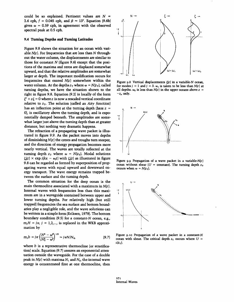
I have made a parallel derivation of the spectra at thetwo turning points (figure 9.11), assuming horizontallyisotropic wave propagation within the entire equatorialwaveguide. It turns out that the buoyancy peak is infact much smaller than the inertial peak at moderatelatitudes. But at very low latitude the inertial peakvanishes. This is in accord with the equatorial obser-vations by Eriksen (1980). Fu (1980) gives an interestingdiscussion of the relative contributions to the spectralpeak at the local inertial frequency co = foca from twoprocesses: (1) local generation of resonant inertial

N i/2

N max 2

.if .2f .5f f 2f 5f

wFigure 9.II Enhancement of the kinetic-energy spectrum(left) and of the potential-energy spectrum (right) at the iner-tial and buoyancy frequencies, respectively. The inertial spec-

.2N .5N N 2N

trum is drawn for latitudes 1°, 5°, 10 °, 30°, 45 °. The buoyancyspectrum is drawn for two depths, corresponding to N = , 4

times the maximum buoyancy frequency.

272Walter Munk

if C- II I �- - - __ _ _�__

waves co = ocal; and (2) remote generation of waves ofthe same frequency o = fiocal at lower latitudes (wheref < focal}. Figure 9.11 is drawn for case 2 under theassumption that the equatorial waveguide is filled withhorizontally isotropic, freely propagating radiation.Take the curve marked 30°, say. Then for o > f astation at lat. 30° is within the equatorial waveguide;for co < f the spectrum is the result of evanescentextensions from a waveguide bounded by lower lati-tudes. Over rough topography and in regions of strongsurface forcing, the case can be made for local genera-tion of the inertial peak. It would seem that the buoy-ancy peak at mid-depth must always be associated withremote generation.

9.5 Shear

Internal waves are greatly modified by an underlyingshear flow.4 A variable U(z) can have a more traumaticeffect on internal waves than a variable Niz). For readycomparison with figure 9.9 showing the effect of avariable N(z) on a traveling wave packet, we havesketched in figure 9.10 the situation for a wave packettraveling in the direction of an increasing U(z). As thewave packet approaches the "critical depth" zc wherethe phase velocity (in a fixed frame of reference) equalsthe mean flow, c = U(zc), the vertical wavenumberincreases without limit (as will be demonstrated).

For the present purpose we might as well avoid ad-ditional complexities by setting f = 0. The theoreticalstarting point is the replacement of Ot by Ot + Ua, +w Oz in the linearized equations of motion. The resultis the Taylor-Goldstein equation [Phillips (1977a, p.248)]:

d% N U" - =dz (U - C)2 U - c =

dzd2Udz 2 I

-oo0

-z

u (z)-0

0

C (z) ~0

I+

Figure 9.I2 First mode vertical displacements (z) in aCouette flow (constant U' and constant N), for U'/N = 0, + 1.Waves move from left to right, and U is positive in the direc-tion of wave propagation. (Thorpe, 1978c.)

-z

U

-h

F

L

N(z) - , U'(z)--0

0 +

o

Do

I

Figure 9.I3 Similar to figure 9.12, but with U' and N confinedto a narrow transition layer.

(9.8)

where c is the phase velocity in a fixed reference frame.(This reduces to

d2 f Nk2_ - o 2

d2 + k2 = 0dz--' + (9.9)

for U = 0.) The singularity at the critical depth whereU = c is in contrast with the smooth turning-pointtransition at N = o; this is the analytic manifestationof the relative severity of the effect of a variable U(z)versus that of a variable N(z).

Thorpe (1978c) has computed the wave function ;(z)for (1) the case of constant N and U' and (2) the casewhere N and U' are confined to a narrow transitionlayer. The results are shown in figures 9.12 and 9.13.The profiles are noticeably distorted relative to the case

273Internal Waves

\

r

-H.

> -·::�:

A

-- UN-

of zero shear, with the largest amplitudes displacedtoward the level at which the mean speed (in the di-rection of wave propagation) is the greatest. Finite-am-plitude waves have been examined for the case 2.Where there is a forward5 flow in the upper level (in-cluding the limiting case of zero flow), the waves havenarrow crests and flat troughs, like surface waves; withbackward flow in the upper layer, the waves have flatcrests and narrow troughs. Wave breaking is discussedlater.

9.5.1 Critical Layer Processes 6

The pioneering work is by Bretherton (1966c), and byBooker and Bretherton (1967). Critical layers have beenassociated with the occurrence of clear-air turbulence;their possible role with regard to internal waves in theoceans has not been given adequate attention.

Following Phillips (1977a), let

ohF =kU + w,co k

= (k2 + m 2 )1 2 = cos

designate the frequency in a fixed reference frame. U(z)is the mean current relative to this fixed frame, andtoF - kU = o is the intrinsic frequency [as in (9.5)], asit would be measured from a reference frame driftingwith the mean current U(z).

Bretherton (1966c) has given the WKB solutions forwaves in an ocean of constant N and slowly varyingU. [It is important to note the simplification to (9.8)when U" = 0 at the critical layer.] Near the criticiallayer depth z,, the magnitudes of w, u, and of the ver-tical displacement vary as

w - IZ - zCl'"', u -IZ - ZC{-1/2,

The quantities OF and k are constant in this problem,but m and ot are not. The vertical wavenumber in-creases, whereas the intrinsic frequency decreases as awave packet approaches its critical layer:

m - Iz - zc,-', ° - Iz - Z.

A sketch of the trajectory is given in figure 9.10. Wavesare refracted by the shear and develop large verticaldisplacements (even though w -- 0), large horizontalvelocities u, and very large induced vertical shears u'.This has implications for the dissipation and breakingof internal waves.

For Ri > , Booker and Bretherton (1967) derived anenergy transmission coefficient

p = exp(-27rRi - ¼). (9.11)

In the usual case, U' << 2N so that Ri >> and p issmall. This is interpreted as wave energy and momen-tum being absorbed by the mean flow at z,. As Ri -+o, p -- 0, consistent with the WKB prediction of Breth-

erton (1966c) that a wave packet approaches but neverreaches the critical layer.

The small coefficient of transmission for Richardsonnumbers commonly found in the ocean implies thatthe critical layer inhibits the vertical transfer of waveenergy. This effect has been verified in the laboratoryexperiments of Bretherton, Hazel, Thorpe, and Wood(1967). When rotation is introduced, the energy andmomentum delivered to the mean flow may altema-tively be transferred from high-frequency to low-fre-quency waves (if the time scales are appropriate). Thusit is possible that some sort of pumping mechanismmay exist for getting energy into, for example, the high-mode, quasi-inertial internal waves. This mechanismcan be compared with McComas and Bretherton's(1977) parametric instability, a weakly nonlinear inter-action (section 9.6).

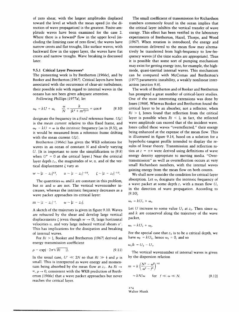
The work of Bretherton and of Booker and Brethertonhas prompted a great number of critical-layer studies.One of the most interesting extensions was done byJones (1968). Whereas Booker and Bretherton found thecritical layer to be an absorber, not a reflector, whenRi > , Jones found that reflection from the criticallayer is possible when Ri < ; in fact, the reflectedwave amplitude can exceed that of the incident wave.Jones called these waves "overreflected," their energybeing enhanced at the expense of the mean flow. Thisis illustrated in figure 9.14, based on a solution for ahyperbolic-tangent profile intended to display the re-sults of linear theory. Transmission and reflection ra-tios at z = + were derived using definitions of waveenergy density appropriate to moving media. "Over-transmission" as well as overreflection occurs at verysmall Richardson numbers, with the internal wavesgaining energy from the mean flow on both counts.

We shall now consider the condition for critical-layerabsorption. Let co, designate the intrinsic frequency ofa wave packet at some depth z, with a mean flow U,in the direction of wave propagation. According to(9.10),

)F = k U + 1.

Let U increase to some value U2 at z2. Then since F

and k are conserved along the trajectory of the wavepacket,

cOF = k U 2 + 02

For the special case that z 2 is to be a critical depth, wehave J)F = kU 2, hence o2 = 0, and so

o/lk = U 2 - U.

The vertical wavenumber of internal waves is givenby the dispersion relation

(N2 - c2) 1/2

m =k ( 2 f2

" kNo for f << c << N. (9.12)

274Walter Munk

I _ �_rlll __ _ I_ ___

- - ZC-1/2.

for critical layer processes as rms u from the internalwaves themselves. The internal wave spectrum is thendivided into two parts: (1) the intrinsic part m < mc,which contains most of the energy, and (2) the com-pliant part m > m,, which is greatly modified by in-teraction with the intrinsic flow field. The phase speedfor critical reflection is

(9.14)CC = rmsu,

and the critical wavenumber is

mc = N/rmsu. (9.15)

Ri

Figure 9.I4 Fractional internal wave energy reflected andtransmitted through a mean shear flow U = Utanh(z/d) atconstant N, as a function of the minimum Richardson numberRi = Nd2/U2o. Internal wave energy is lost to the mean flowfor RI2 + TI 2 < 1, orRi > O.:L8; internal wave energy is gainedfrom the mean flow for R < 0.18. The plot is drawn forRi = 2a2, where a = kd is the dimensionless horizontal wave-number. This corresponds to a wave packet traveling at aninclination of 45° at z = o-. (Ri = a2 corresponds to thelimiting case of vertical group velocity to +x.) (I am indebtedto D. Broutman for this figure.)

There is the separate question whether the internalwaves at the critical layer will be underreflected, justreflected, or overreflected, and this depends on the am-bient Richardson number. In the underreflected casethere is a flux of energy from the compliant to theintrinsic waves. In the overreflected case the flow isthe other way. For an equilibrium configuration, onemay want to look for a transmission coefficient p nearunity, and the exponential behavior of p(Ri) will thenset narrow bounds to the ambient spectrum. But thisgets us into deep speculation, and had better be left tothe end of this chapter.

9.6 Resonant Interactions

For critical absorption within the interval Az overwhich the mean flow varies by A U, we replace co/k byA U, and obtain the critical vertical wavenumber

mc = N/A U. (9.13)

R. Weller (personal communication) has analyzed amonth of current measurements off California for theexpected difference A U =- U2 - U,1 in a velocity com-ponent (either of the two components) at two levelsseparated by Az = z2 - z,. The observations are, ofcourse, widely scattered, but the following values giverepresentative magnitudes:

Az in mAU in cm s-1

0 10 25 500 4 7' 100 7 10 12

10015 (upper 100 m)15 (100-300 m depth)

For AU = 10 cms - 1 and N = 0.01 s- (6 cph), (9.13)gives mc = 10-3 cm-l (16 cpkm). Internal waves withvertical wavelengths of less than 60 m are subject tocritical-layer interactions;.

A large fraction of the measured velocity differenceA U can be ascribed to the flow field u (z) of the internalwaves themselves, and deduced from the model spec-tra. The expected velocity difference increases to /2times the rms value as the separation increases to thevertical coherence scale, which is of order 100 m. Heremost of the contribution comes from low frequenciesand low wavenumbers. I am tempted to interpret A U

Up to this point the only interactions considered arethose associated with critical layers. In the literaturethe focus has been on the resonant interaction of wavetriads, using linearized perturbation theory. There aretwo ways in which critical layer interactions differfrom resonant interactions: (1) compliant waves of anywavenumber and any frequency are modified, as longas c equals u somewhere in the water column; and (2)the modification is apt to be large (the ratio u/c beinga very measure of nonlinearity). For the wave triads,the interaction is (1) limited to specific wavenumbersand frequencies, and (2) assumed to be small in theperturbation treatment. 7 To borrow some words ofO. M. Phillips (1966b), the contrast is between the"strong, promiscuous interactions" in the critical layerand the "weak, selective interactions" of the triads.

The conditions for resonance are

k l + k2 = k, 01 + (02 = (03,

where ki = (k,li, mi), and all frequencies satisfy thedispersion relation wco(k,). Resonant interactions arewell demonstrated in laboratory experiments. For atransition layer (as in figure 9.4), Davis and Acrivos(1967) have found that a first-order propagating mode,which alternately raises and lowers the transitionlayer, was unstable to resonant interactions, leading toa rapid growth of a second-order mode, which alter-nately thickens and thins the transition layer like a

275Internal Waves

propagating link sausage. Martin, Simmons, andWunsch (1972) have demonstrated a variety of resonanttriads for a constant-N stratification.

Among the infinity of possible resonant interactions,McComas and Bretherton (1977) have been able toidentify three distinct classes that dominate the com-puted energy transfer under typical ocean conditions.Figure 9.15 shows the interacting propagation vectorsin (k, m )-space. The associated frequencies o areuniquely determined by the tilt of the vectors, in ac-cordance with (9.4). Inertial frequencies (between f and2f, say) correspond to very steep vectors, buoyancy fre-quencies (between 2N and N) to flat vectors, as shown.

Elastic scattering tends to equalize upward anddownward energy fluxes for all but inertial frequencies.Suppose that k3 is associated with waves generatednear the sea surface propagating energy downward (atright angles to k3, as in figure 9.7). These are scatteredinto k,, with the property m, = -m3, until the upwardenergy flux associated with k, balances the downwardflux by k3. The interaction involves a near-intertialwave k2 with the property m2 2m3. (The reader willbe reminded of Bragg scattering from waves having halfthe wavelength of the incident and back-scattered ra-diation.) Similarly, for bottom-generated k, waves withupward energy fluxes, elastic scattering will transferenergy into k3 waves.

Induced diffusion tends to fill in any sharp cutoffsat high wavenumber. The interaction is between twoneighboring wave vectors of high wavenumber and fre-quency, k, and k3, and a low-frequency low-wavenum-ber vector k2 . Suppose the k2 waves are highly ener-getic, and that the wave spectrum drops sharply forwavenumbers just exceeding Ik3 l, such as Ikll. This in-teraction leads to a diffusion of action (energy/w) intothe low region beyond k31, thus causing k, to grow atthe expense of k2.

Parametric subharmonic instability transfers energyfrom low wavenumbers k2 to high wavenumbers k, ofhalf the frequency, co = 2-, ultimately pushing energyinto the inertial band at high vertical wavenumber.The interaction involves two waves k, and k3 of nearlyopposite wavenumbers and nearly equal frequencies.The periodic tilting of the isopycnals by k2 varies thebuoyancy frequency at twice the frequency of ki andk3 . (The reader will be reminded of the response of apendulum whose support is vertically oscillated attwice the natural frequency.)

The relaxation (or interaction) time is the ratio ofthe energy density at a particular wavenumber to thenet energy flux to (or from) this wavenumber. Theresult depends, therefore, on the assumed spectrum.For representative ocean conditions, McComas (inpreparation) finds the relaxation time for elastic scat-tering to be extremely short, of the order of a period,and so up- and downgoing energy flux should be in

balance. This result does not apply to inertial frequen-cies, consistent with observations by Leaman and San-ford (1975) of a downward flux at these frequencies.The relaxation time for induced diffusion is typicallya fraction of a period! (This is beyond the assumptionof the perturbation treatment.) Any spectral bump isquickly wiped out. The conclusion is that the resonantinteractions impose strong restraints on the possibleshapes of stable spectra.

In a challenging paper, Cox and Johnson (1979)have drawn a distinction between radiative and dif-fusive transports of internal wave energy. In the ex-amples cited so far, energy in wave packets is radiatedat group velocity in the direction of the group velocity.But suppose that wave-wave interactions randomizethe direction of the group velocity. Then eventuallythe wave energy is spread by diffusion rather than ra-diation. The relevant diffusivity is K = (c), where ris the relaxation time of the nonlinear interactions.Cox and Johnson have estimated energy diffusivitiesand momentum diffusivities (viscosities); they findthat beyond 100 km from a source, diffusive spreadingis apt to dominate over radiative spreading. There is aninteresting analogy to crystals, where it is known thatenergy associated with thermal agitation is spread bydiffusion rather than by radiation. The explanation liesin the anharmonic restoring forces between molecules,which bring about wave-wave scattering at room tem-peratures with relaxation times in the nanoseconds.

9.7 Breaking

This is the most important and least understood aspectof our survey. Longuet-Higgins has mounted a broadlybased fundamental attack on the dynamics of breakingsurface waves, starting with Longuet-Higgins and Fox(1977), and this will yield some insight into the inter-nal-wave problems. At the present time we depend onlaboratory experiments with the interpretation of theresults sometimes aided by theoretical considerations.

Figure 9.16 is a cartoon of the various stages in anexperiment performed by Thorpe (1978b). A densitytransition layer is established in a long rectangulartube. An internal wave maker generates waves of thefirst vertical mode. Before the waves have reached thefar end of the tube, the tube is tilted through a smallangle to induce a slowly accelerating shear flow. Theunderlying profiles of density, shear, and vertical dis-placement correspond roughly to the situation in figure9.13.

For relatively steep waves in a weak positive8 shear,the waves have sharpened crests. At the position of thecrest, the density profile has been translated upwardand steepened (B1). There is significant wave energyloss in this development (Thorpe, 1978c, figure 10).

276Walter Munk

-- I - I ·I�----·I