1

The Schrödinger Equation in Three Dimensions Particle in a Rigid Three-Dimensional Box (Cartesian Coordinates) To illustrate the solution of the time-independent Schrödinger equation (TISE) in three dimensions, we start with the simple problem of a particle in a rigid box. This is the three-dimensional version of the problem of the particle in a one-dimensional, rigid box. In one dimension, the TISE is written as

2 2

2

( ) ( ) ( ) ( ).2d x

U x x E xm dx

ψ ψ ψ− + = (1)

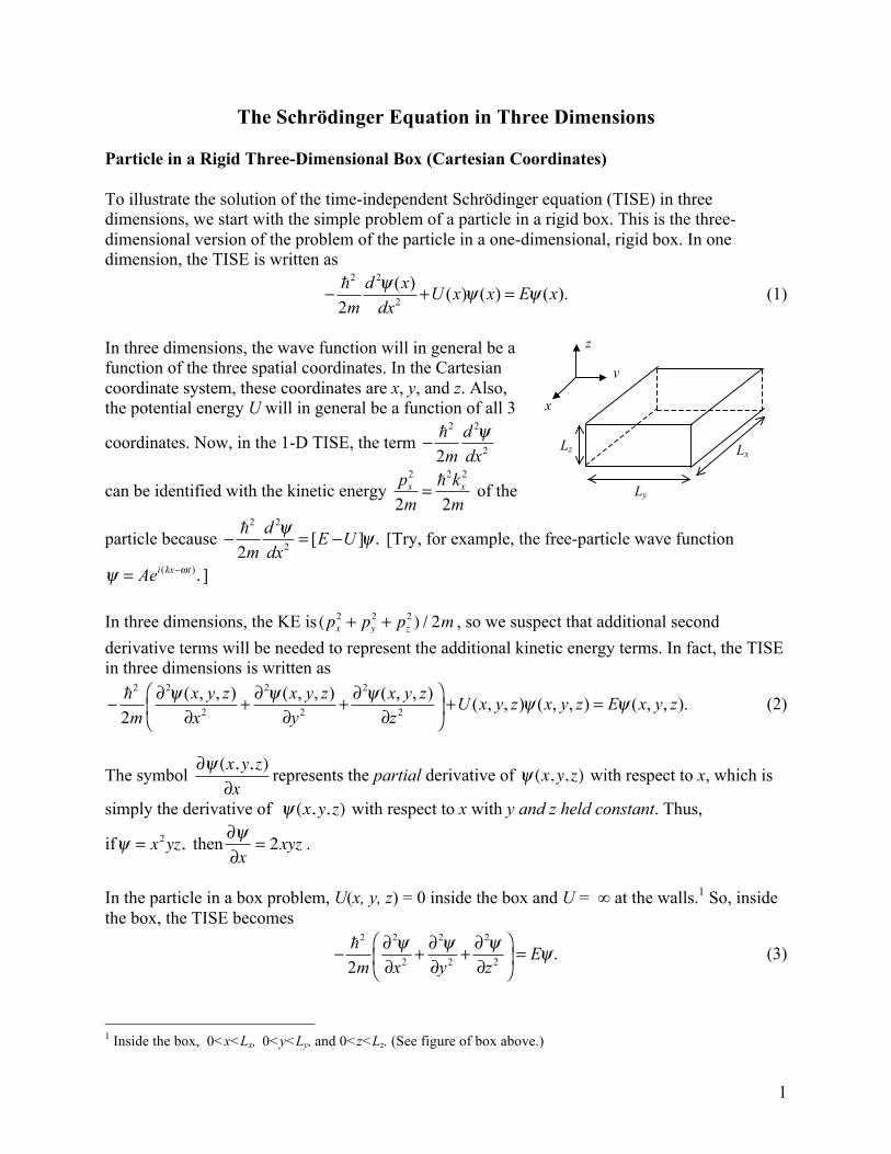
In three dimensions, the wave function will in general be a function of the three spatial coordinates. In the Cartesian coordinate system, these coordinates are x, y, and z. Also, the potential energy U will in general be a function of all 3

coordinates. Now, in the 1-D TISE, the term 2 2

22d

m dxψ−

can be identified with the kinetic energy 2 2 2

2 2x xp km m

= of the

particle because 2 2

2 [ ] .2d

E Um dx

ψ ψ− = − [Try, for example, the free-particle wave function ( ) .i kx tAe ωψ −= ]

In three dimensions, the KE is (px

2 + py2 + pz

2 ) / 2m , so we suspect that additional second derivative terms will be needed to represent the additional kinetic energy terms. In fact, the TISE in three dimensions is written as

2 2 2 2

2 2 2

( , , ) ( , , ) ( , , ) ( , , ) ( , , ) ( , , ).2

x y z x y z x y zU x y z x y z E x y z

m x y zψ ψ ψ ψ ψ

⎛ ⎞∂ ∂ ∂− + + + =⎜ ⎟∂ ∂ ∂⎝ ⎠

(2)

The symbol ∂ψ (x, y, z)

∂xrepresents the partial derivative of ψ (x, y, z) with respect to x, which is

simply the derivative of ψ (x, y, z) with respect to x with y and z held constant. Thus,

ifψ = x2yz, then∂ψ∂x

= 2xyz .

In the particle in a box problem, U(x, y, z) = 0 inside the box and U = ∞ at the walls.1 So, inside the box, the TISE becomes

2 2 2 2

2 2 2 .2

Em x y z

ψ ψ ψ ψ⎛ ⎞∂ ∂ ∂− + + =⎜ ⎟∂ ∂ ∂⎝ ⎠

(3)

1 Inside the box, 0<x<Lx, 0<y<Ly, and 0<z<Lz. (See figure of box above.)

Ly

Lx Lz

z

x

y

2

To solve partial differential equations (the TISE in 3D is an example of these equations), one can employ the method of separation of variables. We write ψ (x, y, z) = X(x)Y (y)Z(z), (4) where X is a function of x only, Y is a function of y only, and Z is a function of z only. Substituting for ψ in Eq. (3) yields

2 2 2 2

2 2 2( ) ( ) ( ) ( ) ( ) ( ) ( ) ( ) ( ).2

d X d Y d ZY y Z z X x Y z X x Y y EX x Y y Z z

m dx dy dz⎡ ⎤

− + + =⎢ ⎥⎣ ⎦

(5)

Note that the partial derivatives have disappeared, since X, Y, and Z are functions of one variable

only. Dividing both sides by 2

( ) ( ) ( )2X x Y y Z z

m− yields

2 2 2

2 2 2 2

1 1 1 2 .d X d Y d Z mEX dx Y dy Z dz

⎡ ⎤+ + = −⎢ ⎥

⎣ ⎦ (6)

For a given solution, E is a constant. Further, note that the first term in the square brackets is a function of x only, the second term is a function of y only, and the third term is a function of z only. For Eq. (6) to be valid for all values of x, y, and z, each of the three terms must be constant. If this were not true, and, for example, all the terms were variable, then if one held y and z constant and changed x, the sum on the left hand side of the equation would change, violating the equation. Eq. (6) therefore becomes three separated ordinary differential equations:

1Xd 2Xdx2

= −k x2 , (7)

1Yd 2Ydy2

= −k y2 , (8)

and

1Zd 2Zdz2

= −k z2 , (9)

with

2 2 22

2 .x y zmE

k k k+ + =

(10)

The separation constants are written as−k x

2 , −k y2 , and −k z

2 in analogy with the 1-D particle in a box problem. Eqs. (7), (8), and (9) are identical to the equation obtained in the 1-D problem and the boundary conditions are the same. For example, X(x) = 0 at x = 0 and x = Lx since the wave functions cannot penetrate the wall. The boundary condition at x = 0 leads to X(x) = A1sin kxx.

The boundary condition at x = Lx leads to kx =nxπLx

, where nx = 1, 2,… Similar solutions are

obtained for Y(y) and Z(z). Hence, we find that

3

ψ (x, y, z) = Asin nxπ xLx

⎛⎝⎜

⎞⎠⎟sin

nyπ yLy

⎛

⎝⎜⎞

⎠⎟sin

nzπ zLz

⎛⎝⎜

⎞⎠⎟, (11)

and from Eq. (10), we find the energy

22 22 2

.2

yx z

x y z

nn nE

m L L Lπ ⎡ ⎤⎛ ⎞⎛ ⎞ ⎛ ⎞⎢ ⎥= + +⎜ ⎟⎜ ⎟ ⎜ ⎟⎜ ⎟⎢ ⎥⎝ ⎠⎝ ⎠ ⎝ ⎠⎣ ⎦

(12)

The integers nx, ny, and nz are called quantum numbers. These quantum numbers specify the quantum states of the system. Thus, we can label the wave functions and energies according to the values of the quantum numbers: ψ nxnynz

; Enxnynz.

The ground state energy is

22 22 2

1111 1 1 .

2 x y z

Em L L Lπ ⎡ ⎤⎛ ⎞⎛ ⎞ ⎛ ⎞⎢ ⎥= + +⎜ ⎟⎜ ⎟ ⎜ ⎟⎜ ⎟⎢ ⎥⎝ ⎠⎝ ⎠ ⎝ ⎠⎣ ⎦

(13)

If the box is a cube, then Lx = Ly = Lz = L, and the energy becomes

( )2 2

2 2 22 .

2x y zn n n x y zE n n nmLπ= + + (14)

The ground state energy is then 2 2

111 2

3 .2

EmLπ=

Degeneracy For the next higher energy level up from the ground state, there are 3 distinct wave functions or quantum states of the cubical box that have this energy:ψ 211, ψ 121, ψ 112 . These quantum states are distinct because their probability densities are different. (E.g.,

ψ 2112 = A 2 sin2 2π x

L⎛⎝⎜

⎞⎠⎟sin2 π y

L⎛⎝⎜

⎞⎠⎟sin2 π z

L⎛⎝⎜

⎞⎠⎟≠

A 2 sin2 π xL

⎛⎝⎜

⎞⎠⎟sin2 2π y

L⎛⎝⎜

⎞⎠⎟2

sin2 π zL

⎛⎝⎜

⎞⎠⎟= ψ 121

2 .) The occurrence of more than one distinct

quantum states (wave functions) with the same energy is called degeneracy. In the case of the particle in a rigid, cubical box, the next-lowest energy level is three-fold degenerate.

2 2

211 121 112 2

3 .E E EmLπ= = = (15)

. Note that the ground state is non-degenerate. Further, the three-fold degeneracy of the first-excited state is removed if Lx ≠ Ly ≠ Lz . Degeneracy is intimately connected to symmetry: the

4

greater the symmetry of the system, the higher the degeneracy of the quantum states. [See www.falstad.com for simulations.] Contour Maps Contours represent lines of equal probability density. See the contour maps for the 2-D rigid box in the Taylor et al. textbook. The Three Dimensional Central-Force Problem Ultimately, our aim is to solve the TISE for an atomic system. The simplest atomic system is a one-electron atom in which a single electron is bound to the nucleus. In this case, the potential energy

U(x, y, z) =U(r) = −kZe2

r. (16)

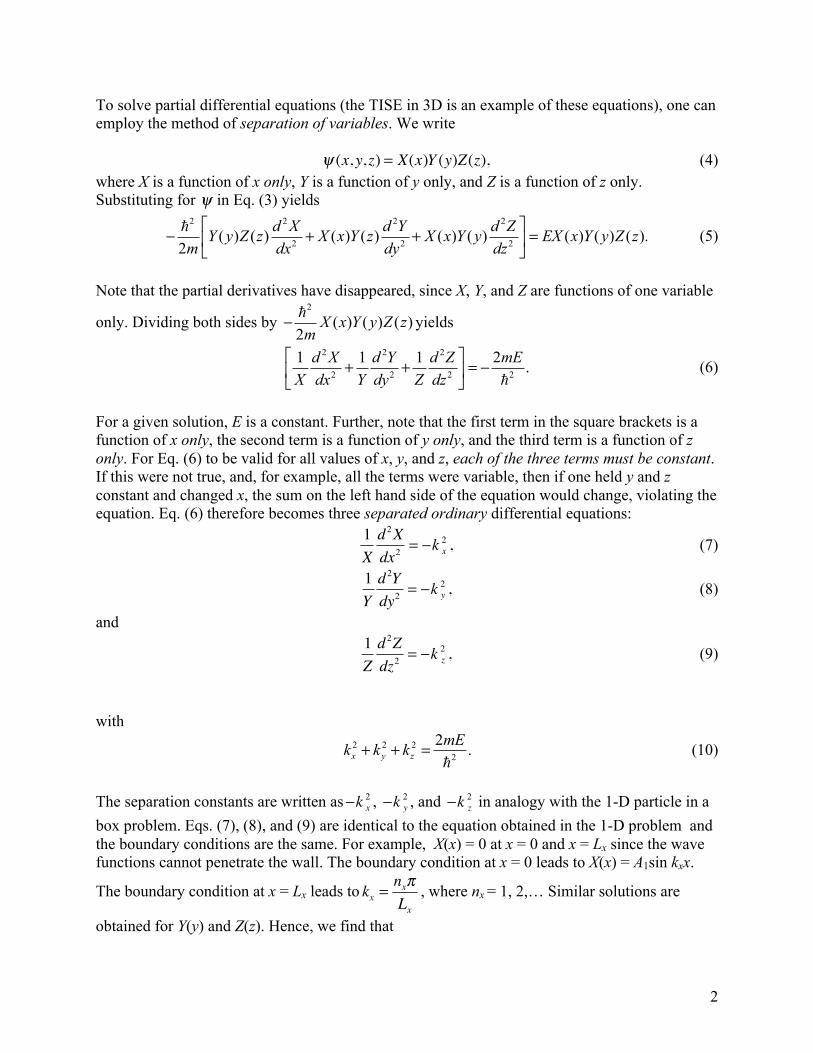
The potential energy is a function of only the radial distance r. The corresponding force is directed along –

r . Such a force (in this case, the electrostatic force) is called a central force. Note that U is spherically symmetric since it depends only on r. Thus, classically, in a one-electron atomic system in which no external forces act, one does not expect the energy E to depend on the angular position of the electron, only on the radial distance from the nucleus. Because of the spherical symmetry, the solution to the TISE is tractable if we use spherical polar coordinates rather than Cartesian coordinates. In the spherical coordinate system, the coordinates are r, θ, andφ , where r is the radial distance, θ is the polar angle, and φ is the azimuthal angle. For a spherically symmetric potential energy U(r), the TISE cannot be solved using separation of variables in Cartesian coordinates. In spherical coordinates, however, the TISE is separable, and this is the solution we shall study. It turns out that even though the TISE is separable in spherical coordinates, the solution is complicated and we shall not go into all the mathematical details of the solution. Rather, we shall concentrate on the physics. In spherical coordinates, the TISE for a spherically symmetric potential is given by

2 2 2

2 2 2 2 2

1 1 1( ) sin ( ) ,2 sin sin

r U r Er r r r

ψ ψψ θ ψ ψµ θ θ θ θ φ⎛ ⎞∂ ∂ ∂ ∂⎛ ⎞− + + + =⎜ ⎟⎜ ⎟∂ ∂ ∂ ∂⎝ ⎠⎝ ⎠

(17)

+Ze

–e

z

y

x

r

P

φ

θ

cos siny r θ φ=

cos cosx r θ φ=

cosz r θ=

5

where ψ ≡ψ (r,θ,φ)and the mass is taken to be the reduced massµ . [Recall that this accounts for the slight motion of the nucleus.] Using separation of variables, we seek a solution of the form ψ (r,θ,φ) = R(r)Θ(θ)Φ(φ). (18) Substituting in the TISE and separating yields

1Φd 2Φdφ 2

= −ml2 , (19)

1sinθ

ddθ

sinθ dΘdθ

⎛⎝⎜

⎞⎠⎟+ l(l +1) − ml

2

sin2θ⎡

⎣⎢

⎤

⎦⎥Θ = 0, (20)

and

2 2

2 2 2

2 ( 1)( ) ( ) 0,2

d l lrR U r E rRdr r

µµ

⎡ ⎤+− + − =⎢ ⎥⎣ ⎦

(21)

where in Eq. (19), the separation constant is 2m− and in Eq. (20), the separation constant is l(l +1) . Note that neither the θ nor the φ equation contains U(r). Thus, these equations are valid for all central force potential energies.

We can solve Eq. (19) easily. We first rewrite it as d 2Φdφ 2

+ ml2Φ = 0, the solution of which is

Φ = Aeiml (φ+δ ). (22) In Eq. (22), A and δ are integration constants. The boundary condition is that Ф has to be single-valued, i.e., Φ(φ) = Φ(φ + 2πn),where n is an integer. This means that ei(2πnml ) = 1, (23) i.e., ml = 0, ±1, ± 2,... (24) Angular Momentum The angular wave function Φ = Aeimlφ reminds us of the 1-D free-particle wave function (time suppressed) ψ (x) = Beikx , which we can write as /( ) ipxx Beψ = , where p k= is the particle's linear momentum. Similarly, we can write /( ) ziLAe φφΦ = , where .z lL m= is the z-component of the angular momentum. The important thing to note is that Lz is quantized for a particle with angular wave function Ф, i.e., it can assume only discrete values lm , where ml = 0, ±1, ±2, … is the quantum number associated with Lz (magnetic quantum number). In separating the θ-dependent part of the TISE, the separation constant was taken to be l(l+1). It turns out that the solutions to the θ-equation, i.e., the Θ(θ), are of two kinds. One kind remains finite for all 0 ≤ θ ≤ π for non-negative integer values of l and the other kind blows up at θ = 0 and π. Thus, only in the case of the first kind will physically meaningful solutions be obtained. The θ-equation is known as the associated Legendre equation, and the physically acceptable

6

solutions are the associated Legendre functions of the first kind,Plml (θ) . Note that these functions

depend on both l and ml. In fact, the solutions impose the condition l ≥ ml . The physical interpretation of this is that the magnitude of the orbital angular momentum

L is quantized for a

particle with angular wave functionΘ(θ) : ( 1) ,L l l= +

(25)

or, 2 2( 1) . ( 0, 1, 2,...)L l l l= + = (26) The integer l is the orbital angular momentum quantum number. As seen before, the z-component of

L is quantized according to

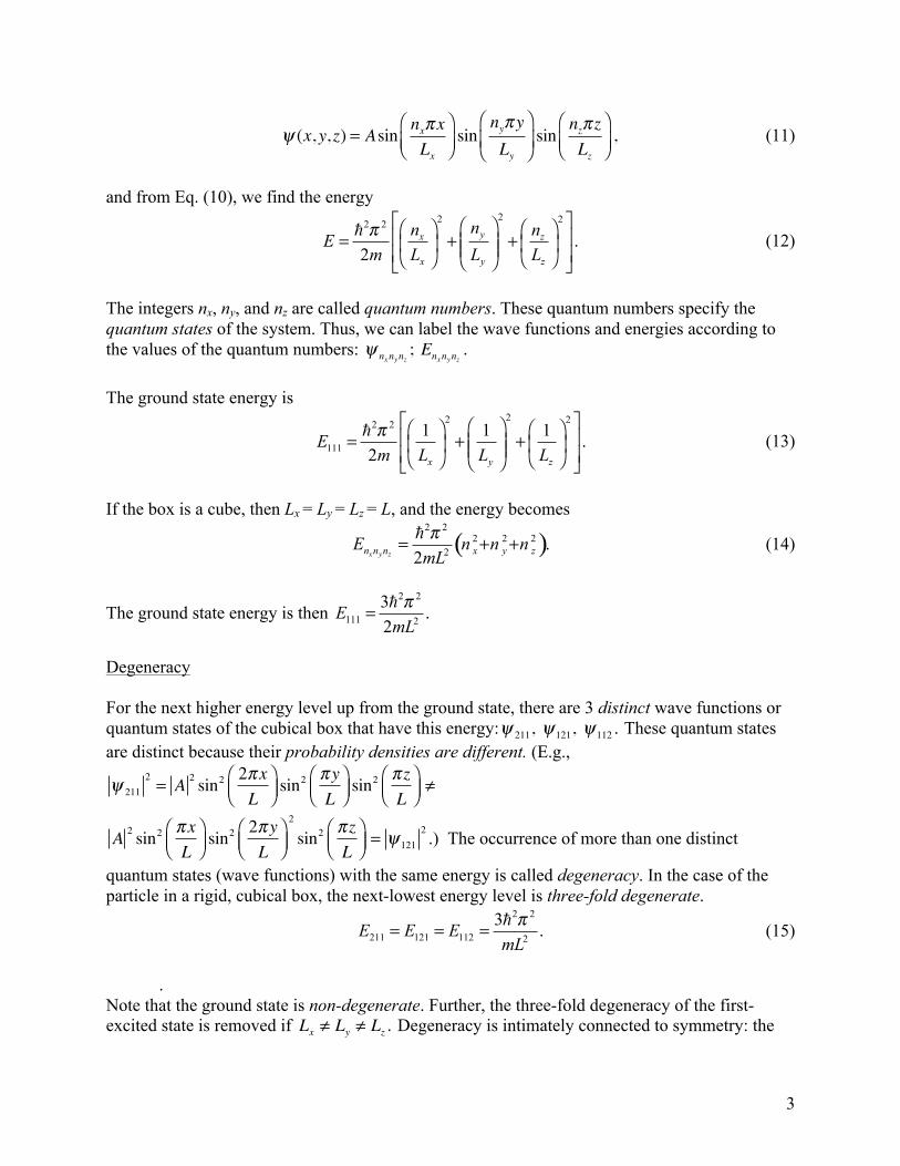
. ( , 1,..., 1, )z l lL m m l l l l= = − − + − (27) Vector Model To visualize the implications of angular momentum quantization, a classical picture, i.e., the vector model, is quite useful. If θ is the polar angle that

L makes with the z-axis, then

cos .( 1) ( 1)l lz m mL

L l l l lθ = = =

+ +

(28)

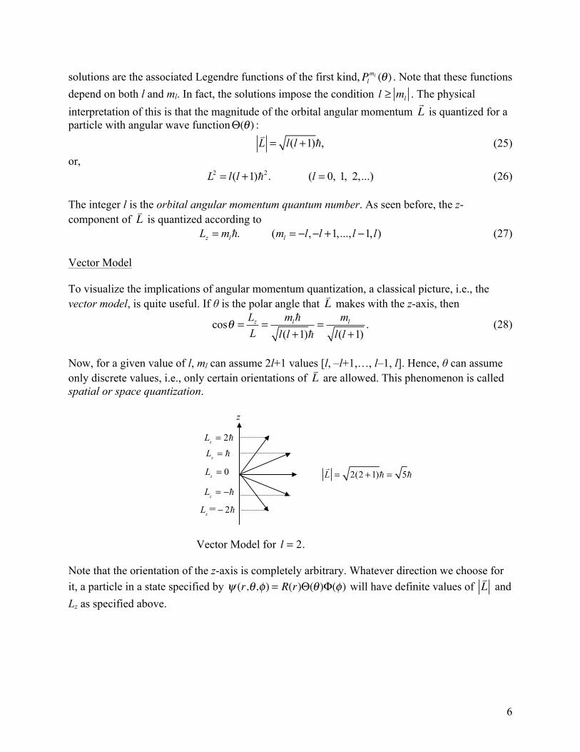
Now, for a given value of l, ml can assume 2l+1 values [l, –l+1,…, l–1, l]. Hence, θ can assume only discrete values, i.e., only certain orientations of

L are allowed. This phenomenon is called

spatial or space quantization.

Vector Model for l = 2. Note that the orientation of the z-axis is completely arbitrary. Whatever direction we choose for it, a particle in a state specified by ψ (r,θ,φ) = R(r)Θ(θ)Φ(φ) will have definite values of

L and

Lz as specified above.

z

2(2 1) 5L = + =

2zL =

zL =

0zL =

2=zL − zL = −

7

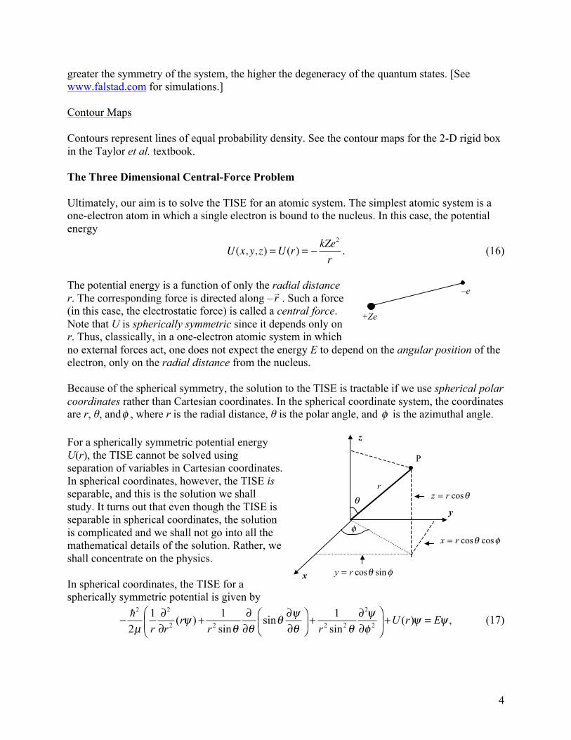
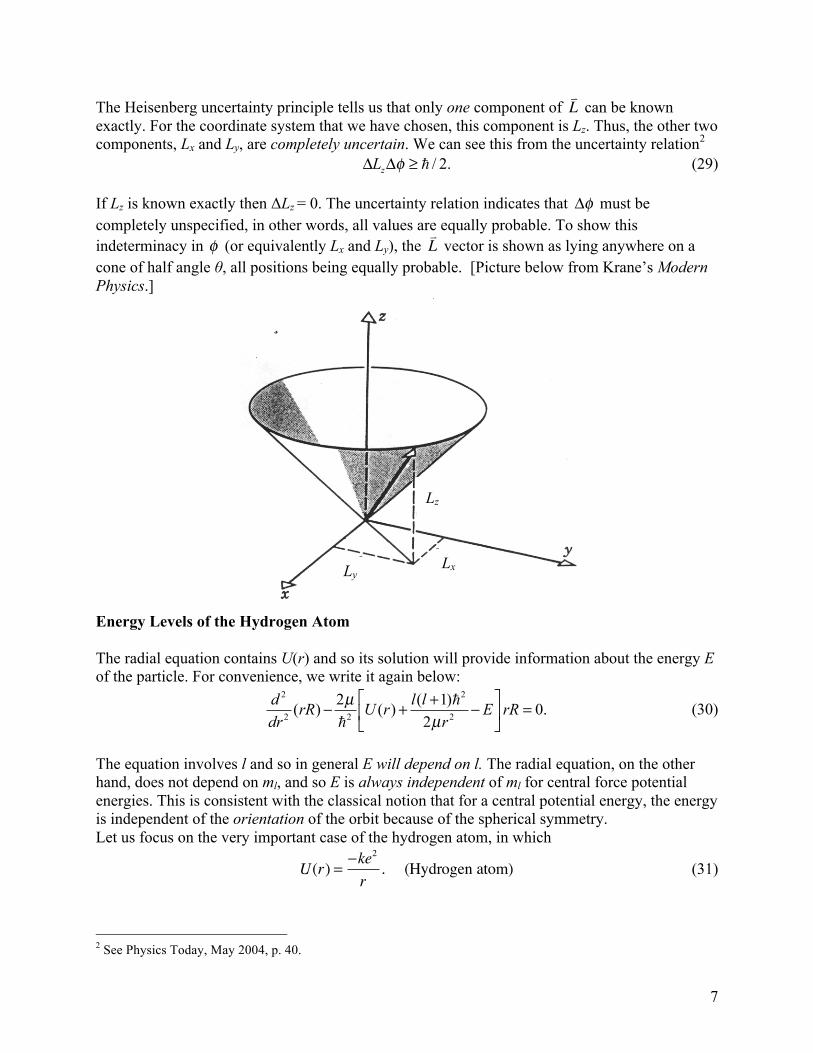
The Heisenberg uncertainty principle tells us that only one component of L can be known

exactly. For the coordinate system that we have chosen, this component is Lz. Thus, the other two components, Lx and Ly, are completely uncertain. We can see this from the uncertainty relation2 / 2.zL φΔ Δ ≥ (29) If Lz is known exactly then ΔLz = 0. The uncertainty relation indicates that Δφ must be completely unspecified, in other words, all values are equally probable. To show this indeterminacy in φ (or equivalently Lx and Ly), the

L vector is shown as lying anywhere on a

cone of half angle θ, all positions being equally probable. [Picture below from Krane’s Modern Physics.]

Energy Levels of the Hydrogen Atom The radial equation contains U(r) and so its solution will provide information about the energy E of the particle. For convenience, we write it again below:

2 2

2 2 2

2 ( 1)( ) ( ) 0.2

d l lrR U r E rRdr r

µµ

⎡ ⎤+− + − =⎢ ⎥⎣ ⎦

(30)

The equation involves l and so in general E will depend on l. The radial equation, on the other hand, does not depend on ml, and so E is always independent of ml for central force potential energies. This is consistent with the classical notion that for a central potential energy, the energy is independent of the orientation of the orbit because of the spherical symmetry. Let us focus on the very important case of the hydrogen atom, in which

U(r) = −ke2

r. (Hydrogen atom) (31)

2 See Physics Today, May 2004, p. 40.

Lz

Lx Ly

8

The resulting radial equation can be solved analytically, and for physically meaningful bound-state solutions satisfying the requisite boundary conditions (R 0→ as r→∞ , which is equivalent to normalizability), one finds quantized energies:

2 2

2 2 2

( ) 1 13.6 eV . (Hydrogen atom)2keE

n nµ= − = −

(32)

The number n is a third quantum number called the principal quantum number, which can assume the integer values n = 1, 2, 3, …. The physically acceptable solutions to the radial equation also require that l can have the values3 l = 0,1, 2, ..., n −1. (Hydrogen atom) (33) The solutions to the radial equation are the radial functions Rnl(r), which are related to the associated Laguerre functions. Notice that E is independent of ml and l. The independence of l is a special characteristic of the 1/r potential energy. We shall see that in the case of multielectron atoms in which the potential is approximately central but not 1/r, E does in fact depend on l. It is also important to note that the energy levels predicted by the TISE are exactly the same as those predicted by the Bohr model, which are known to be correct for the hydrogen atom. The values of the quantum numbers n, l, and ml arose from boundary conditions on the separated functions Rnl, Θlml

, and Φml. The complete wave function for the hydrogen atom is then

ψ nlm (r,θ,ψ ) = Rnl (r)Θml(θ)Φml

(φ). (34) The product of Θlml

(θ) and Φml(φ) is called the spherical harmonics:

Ylml(θ,φ) = Θml

(θ)Φml(φ). (35)

Each quantum state is uniquely specified by the values of the three quantum numbers. Atomic states are labeled with a number-letter code which specifies the values of the quantum numbers n and l. This labeling is known as spectroscopic notation. The number in the code is the value of n. The letter that follows designates the value of l: l = 0 is designated by s (sharp); l = 1 by p (principal), l = 2 by d (diffuse); and l = 3 by f (fundamental). For higher values of l, the code continues alphabetically, e.g., l = 4 is designated by g, l = 5 by h, and so on. We shall use spectroscopic notation to label the wave functions corresponding to each quantum state of the hydrogen atom and construct an energy-level diagram showing the ordering of the energies of the quantum states. We start with the ground state. In the ground state of the H atom, n = 1. This implies that l = 0 and ml = 0. Thus, the ground state is the 1s state. Note also that the ground state is non-degenerate, i.e., the degeneracy = 1, since l = ml = 0.4 For n = 2, l can have two values: 0 and 1. For l = 0, ml = 0 and this is the 2s state. For l = 1, we have three possible value of ml: -1, 0, +1. Hence, there are three 2p states. We see that there are four wave functions (quantum states) for n

3 l has to be limited because for a given energy the angular momentum cannot be arbitrarily large. 4 Note that L = 0 for ground state which differs from Bohr model prediction of L= , The TISE’s value is supported by experiment. Also, actually, there is a degeneracy due to spin.

9

= 2. All four states have the same energy, since E is independent of l and ml. Hence, the energy level for n = 2 (first excited state) is four-fold degenerate. For n = 3, we have one 3s state, three 3p states and five 3d states [ml = -2, -1, 0, +1, +2]. Thus, the degeneracy of the n = 3 energy level is 1+3+5 = 9. In general, the degeneracy of the nth energy level is n2. [Show picture from Taylor et al.] We shall now investigate the probability densities of hydrogenic wave functionsψ nlml

(r,θ,φ) . Hydrogen Atom Wave Functions – Probability Densities In three dimensions, the probability density is a probability per unit volume. Hence, the probability of finding the electron in a volume element dV at position (r, θ,φ ) is

dP(r,θ,φ) = ψ nlml

2dV

= Rnl (r)2 Θlml

(θ)2Φml

(φ)2r2 sinθdrdθdφ. (36)

Notice that

Φml(φ)

2= A 2 eimlφ

2= A 2 . (37)

Hence, the probability of finding the electron within dV at a specified position is always independent of φ. It is very useful to examine the probability that the electron is at a certain distance r from the nucleus, regardless of the values of θ andφ . More precisely, we wish to find the probability that an electron is between r and r +dr, i.e., within the volume of a thin spherical shell. To do this, we first find the volume dV of the spherical shell and then multiply it by Rnl (r)

2 . Now for a spherical shell, dV = 4πr2dr. (38) Then, the required probability is given by P(r)dr = R(r) 2 4πr2dr, (39) where P(r) = 4πr2 R(r) 2 (40) is the radial probability density. [Show picture, Krane, p. 185] Example: (Example 7.3, Krane) Prove that the most likely distance from the origin of an electron in a n = 2, l =1 (2p) state of H atom is 4aB.

10

Solution: P(r) = 4πr2 R21

2 . Since we wish to find the value of r where P(r) is maximized, we need to find dP(r)dr

and set if equal to zero. Now P(r) = (const.) r4e−r /aB . [The multiplicative constants are not

important in solving dP(r)dr

= 0 .] Thus dP(r)dr

= C 4r3e−r /aB + r4 −1aBe−r /aB

⎛⎝⎜

⎞⎠⎟

⎡

⎣⎢

⎤

⎦⎥ = 0.

Thus, Cr3e−r /a0 4 − ra0

⎡

⎣⎢

⎤

⎦⎥ = 0 , i.e., r = 0, ∞ , or r = 4aB. Obviously, r = 0 or ∞ do not give a

maximum, since P(r) = 0 at those values of r. We conclude that P(r) is maximum when r = 4aB. [Show picture, p. 185, Krane (again); Eisberg & Resnick.] In general, as n increases, the position of the highest peak of P(r), i.e., the most probable radial distance for the electron, moves to larger values. The electron is therefore farther from the nucleus on average. This can also be seen by calculating the expectation value of r:

r = r0

∞

∫ P(r)dr. (41)

[Show Figs. in Taylor et al. and Eisberg & Resnick.] While r and rmp (most probable) are certainly different for the various states corresponding to the same n (e.g., 2s, 2p), this variation is relatively small compared to the variation in r (and rmp) for different n. Hence, one can identify a spatial shell with each n. A shell represents a range of distances within which the electron is most likely to be found. [Show diagram.] For example, if the electron is in a quantum state for which n = 2, it is very likely to be found in the n = 2 spatial shell. One can also specify “energy shells” which are groups of quantum states with similar energies. In the H atom (and all one-electron atoms), energy shells and spatial shells are identical because of the degeneracy of the levels for each n. However, in multielectron atoms, E does depend on l quite strongly in some cases, and states with different n can have similar energies. Angular Probability Density As remarked previously, s states have l = 0 and ml = 0. Mathematically, this means the functions

( ) and ( )l lm mθ φΘ Φ are both constants, i.e., independent of θ and φ , respectively. Hence,

ψ n00 has only a radial dependence and so is spherically symmetric. This means the probability

density ψ n002 is spherically symmetric. Physically, l = ml = 0 implies that L = 0, i.e., the

electron has zero angular momentum. L = 0 is consistent with spherically symmetry, since the L

vector picks out a direction in space. Classically, L is fixed and perpendicular to the plane of the

orbit for central force motion. Hence, specifying L immediately tells you the plane of the orbit.

In quantum mechanics, L cannot be precisely specified according to the uncertainty principle,

11

but if it is non-zero, ψ nlml

2will no longer be spherically symmetric (the “orbit” becomes more

planar). Recall, however, that the probability density ψ nlml

2 is always independent ofφ .

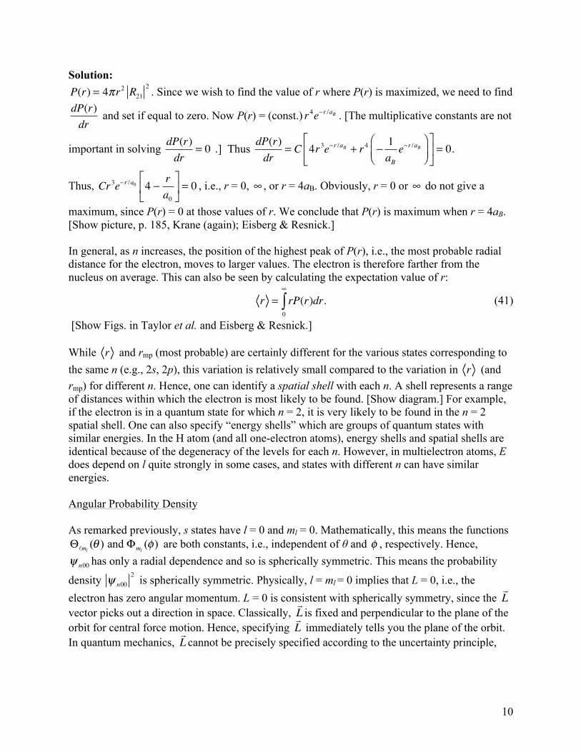
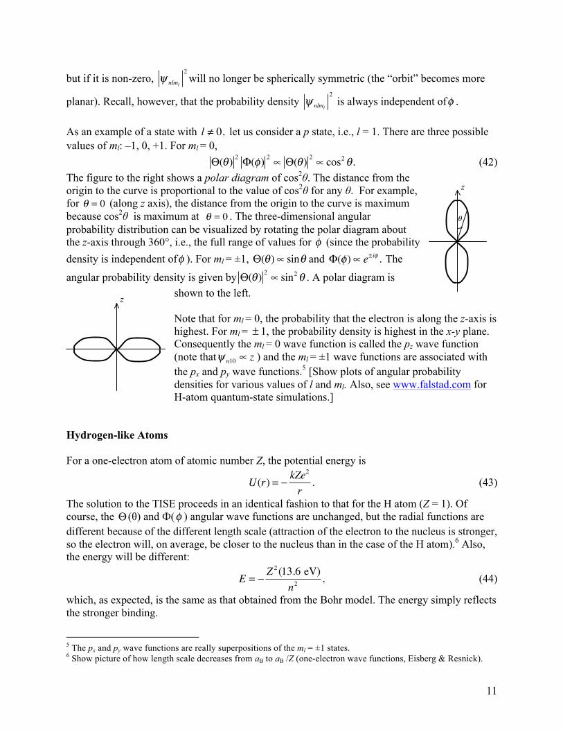
As an example of a state with l ≠ 0, let us consider a p state, i.e., l = 1. There are three possible values of ml: –1, 0, +1. For ml = 0, Θ(θ) 2 Φ(φ) 2 ∝ Θ(θ) 2 ∝ cos2θ. (42) The figure to the right shows a polar diagram of cos2θ. The distance from the origin to the curve is proportional to the value of cos2θ for any θ. For example, for θ = 0 (along z axis), the distance from the origin to the curve is maximum because cos2θ is maximum at θ = 0 . The three-dimensional angular probability distribution can be visualized by rotating the polar diagram about the z-axis through 360°, i.e., the full range of values for φ (since the probability density is independent ofφ ). For ml = ±1, Θ(θ)∝ sinθ and Φ(φ)∝ e± iφ . The

angular probability density is given by Θ(θ) 2 ∝ sin2θ . A polar diagram is shown to the left. Note that for ml = 0, the probability that the electron is along the z-axis is highest. For ml = ± 1, the probability density is highest in the x-y plane. Consequently the ml = 0 wave function is called the pz wave function (note thatψ n10 ∝ z ) and the ml = ±1 wave functions are associated with the px and py wave functions.5 [Show plots of angular probability densities for various values of l and ml. Also, see www.falstad.com for H-atom quantum-state simulations.]

Hydrogen-like Atoms For a one-electron atom of atomic number Z, the potential energy is

U(r) = −kZe2

r. (43)

The solution to the TISE proceeds in an identical fashion to that for the H atom (Z = 1). Of course, the Θ (θ) and Ф(φ ) angular wave functions are unchanged, but the radial functions are different because of the different length scale (attraction of the electron to the nucleus is stronger, so the electron will, on average, be closer to the nucleus than in the case of the H atom).6 Also, the energy will be different:

E = −Z 2 (13.6 eV)

n2 , (44)

which, as expected, is the same as that obtained from the Bohr model. The energy simply reflects the stronger binding.

5 The px and py wave functions are really superpositions of the ml = ±1 states. 6 Show picture of how length scale decreases from aB to aB /Z (one-electron wave functions, Eisberg & Resnick).

z

θ

z