The scenario of two-dimensional instabilities of the ... · actuators, dielectric barrier discharge (DBD) type. EHD actuators can add momentum to the ow around an object in regions

6th Theoretical Fluid Mechanics Conference, June 27-30, 2011, Honolulu, HI

The scenario of two-dimensional instabilities of the

cylinder wake under EHD forcing: A linear stability

analysis

Juan D’Adamo‡, Leo M. Gonzalez†, Alejandro Gronskis‡, and Guillermo Artana‡

†Canal de Ensayos Hidrodinamicos, School of Naval Arquitecture, Universidad Politecnica de Madrid, Spain‡Laboratorio de Fluidodinamica. Facultad de Ingenierıa. Universidad de Buenos Aires, Argentina

Abstract

We propose to study the stability properties of a wake air flow forced by electrohydrodynamic (EHD)actuators, dielectric barrier discharge (DBD) type. EHD actuators can add momentum to the flow aroundan object in regions close to the wall. As the forcing frequencies, characteristic of DBD, are much higherthan the natural shedding frequency of the flow (kHz vs. Hz), we consider in this work the forcing actuationas stationary. The actuators are disposed symmetrically near the boundary layer separation point.We study the flow around a cylinder modified by EHD actuators experimentally by means of particle imagevelocimetry (PIV) measures and also computationally by solving the generalized eigenvalue problem obtainedfrom linearized Navier-Stokes equations. In the numerical part, the presence of the EHD actuators has beenimplemented as a boundary condition on the cylinder surface. The base flow obtained computationallyusing this boundary condition has been compared with the experimental one in order to match the controlparameters from both methodologies. Once the base flow agreement has been verified, the Hopf bifurcationproduced when the flow starts the vortex shedding has been studied by different methods: first, when thebaseflow is obtained from experimental snapshots, the evolution of the amplitude velocity oscillations ismonitored; second, when the baseflow is computationally obtained, a global linearized eigenvalue problem issolved for the instability study. Finally, the critical parameters have been compared.

I. Introduction.

The simply geometry and the complex behavior that exhibits the flow around a cylinder represents, forlow Reynolds numbers (Re = U0D/ν < 190), a prototypical 2D wake flow. The regime is identified withthe Benard von Karman (BvK) vortex street, when the flow breaks its time continuous invariance at thebifurcation Re = 48.5. In this case, the velocity field in the whole flow domain oscillates with the same globalfrequency and its harmonics, related to the appearance of a sufficiently large region of absolute instabilityin the near wake. As the oscillation amplitudes depend on the monitored position, the area that containsnon zero oscillation amplitude points defines an instability region. Previous studies Zielinska et al.1 andWesfreid et al. (1996),2 characterized the behavior of this region determining scale laws for its nonlinearevolution as functions of the Reynolds number.The flow features can be altered by forcing parameters that may be varied smoothly and accurately to giverise different regimes. In this sense, we study this benchmark in order to characterize flow control in wakesby means of electrohydrodynamical actuators (EHD). EHD actuators for flow control have been receivingspecial attention in the last years, as reviewed by Moreau (2007).3 Among all the types of low-energy plasmaactuators, one can notice a group of actuators that produces surface discharges. With these devices the goalis usually to use an electric wind produced by the plasma in order to modify the properties of the boundarylayer close to the wall. A particular type of discharge is the surface dielectric barrier discharge (DBD). This

1 of 18

American Institute of Aeronautics and Astronautics

discharge has been perfected for the first time in air at atmospheric pressure by Masuda(1979)4 for ioniccharging of particles. Roth (1998) et al. used it for airflow applications at the end of the 1990s,5 characterizingthe momentum injected for flat plate and airfoil flows. Later, Thomas et al.(2006)6 applied the DBD for thebluff body flow control. In their results, the authors showed drastic reductions of the flow separation andthe associated Karman vortex shedding. On the other hand, some hypothesis on the dynamics of the DBDforcing arose from a computational study validated with PIV experiments in Gonzalez et al.(2009).7 Froma stability analysis for a bluff body flow, with no vortex shedding, the forcing is introduced numerically as amoving surface boundary condition. In this line, the work by Gronskis (2009)8 analyzed numerical modelsfor DBD forced flows for a cylinder at low Reynolds numbers (Re < 200).We intend with this work to optimize the DBD control device by analyzing the stability properties of the flow.For this reason, we study the possibility of suppressing the vortex sheading when a DBD actuator controlsthe flow. The work has been carried out from both experimental and computational points of view. Globalmodes evolves as the mean flow is modified by external parameters, Barkley (2006)9 introduced hypothesisto consider the mean flow as a base flow for 2D stability analysis. In this way, the mean flow representsa marginal stability state and defines the frequency and amplitude of the wake oscillations. The nonlinearsaturation of the oscillatory instability is achieved by Reynolds stresses from the mean flow modification.Khor et al. (2008)10 and Leontini et al. (2010)11 support these hypothesis from experimental and numericaldata for Re up to 600. These ideas have been applied to analyze forced wakes. Previous studies on thestability properties of forced wakes, Thiria and Wesfreid (2007)12(2009),13 confirmed that a nonlinear criticalbehavior takes place under forcing. Indeed, a bifurcation scenario reappears as the forcing action stabilizesthe wake fluctuations, in their case, a rotary oscillation. Figure 1, adapted from,12 shows how the globalmodes develop under forcing. The control actuation is represented by a vertical line for Re > Rec, thatvaries the reverse flow region when it is present.An interesting interpretation of the influence of a generic slip boundary condition on the wake dynamics wasdone by Legendre in,14 where shedding transition is interpreted as a critical accumulation of surface vorticity.In this context, we pursue the characterization of the DBD control actuator to complete an understandingwhich will eventually lead to a more effective energy consumption. We organize the work as it follows:in section II we describe the experimental setup to produce the DBD discharge as well as the method tomeasure the velocity fields of the flow, in section III we detail the characteristics of the problem, boundaryconditions and baseflow properties, in section IV the numerical methodology to perform the linear global isdescribed, in section V the results obtained in both approaches are shown and compared, at last we resumesome conclusions and formulate perspectives for future works.

Figure 1. The reverse flow region LR behind the cylinder evolves nonlinear with Re, as it is modified by themean flow. A new bifurcation scenario appears under forcing conditions.

II. Experimental setup.

The experimental set-up consists of a flow around a circular cylinder at low Reynolds number, Re ∼ 200.The velocity field measurements were undertaken with the cylinder placed in a closed loop wind tunnel with

2 of 18


a test section of 50× 50cm2, where the air velocity is Uo ' 0.17 m/s.The EHD actuator was mounted on the surface of a polymethyl methacrylate cylinder tube with external

diameter D =20 mm. The tube wall was 2 mm thick.

Figure 2. Schematic of the EHD actuator: Electrodes disposed flush-mounted. Electric circuit and inputsignal detail.

The electric circuit is composed of a signal generator, an audio amplifier and an ignition coil to give adischarge at VEHD = 10kV and a frequency of fEHD = 5.6 kHz. The signal amplitude is then modulated bybursting the signal as showed by Figure 2. A second frequency arises fBurst = 1/TBurst and the electricalenergy delivered by the device is characterized by a duty cycle (DC = T1/TBurst). Special care was takento assure a stationary input as fBurst fflow, being fflow the vortex shedding frequency (' 1.5Hz, as theStrouhal number St = fD/U0 ' 0.2). In short, the flow control parameter is the Duty Cycle (DC) inputthat modulates the ”ionic wind” momentum.

(a) No forcing. (b) Flow under DBD actuation.

Figure 3. Instantaneous PIV velocity fields. The region of interest contains 140×86 vectors, scaled to representthe flow more clearly. Contour levels corresponds to the velocity modulus.

Quantitative measurements were performed using 2D Particle Image Velocimetry (PIV) on a verticalplane placed at mid-span of the cylinder. Image acquisition and PIV calculation were done using a LaVisionsystem, composed of an ImagerPro 1600×1200 CCD camera with a 12-bit dynamic range capable of recordingdouble-frame pairs of images at ∼ 8Hz and a two rod Nd:YAG (15mJ) pulsed laser synchronized by acustomized PC using LaVision DaVis 7.1 software. Laser sheet width was about 1mm in the test section.The whole 300mm × 200mm imaging region (about 12× 8D) gives a spatial resolution of 0.06D as showedin Figure 3. All image acquisitions where done using the double-frame mode with a time lapse between thetwo frames (dt) set to 7ms.Given the flow natural frequency, its dynamic behavior is well resolved by the PIV measures for the selected

3 of 18


acquisition frequency.

III. Problem definition.

The geometry has been non-dimensionalized with the cylinder diameter D. The computational geometryis defined by a rectangle placed with dimensions L = 20 and H = 49. The center of the cylinder is placed atthe middle of the box and 8 units ahead of the inflow boundary, see figure 4.

Figure 4. Computational setup: dimensions and boundary conditions.

The plasma actuation takes place in a thin layer compared to cylinder diameter. This enables to subdividethe problem into two main regions. An inner region where the forcing occurs and an outer region (where wewill perform the numerical simulations) in which electric forces can be disregarded. A kinematic compatibilitycondition can be imposed at the boundary separating both regions. We assume in our case that normalvelocity is null and that no discontinuity in tangential velocities exists. We further assume that the law thatquantifies the tangential velocity distribution is governed from the parameters that determine the dischargein the inner region. In this work no modeling of the inner region based on plasma physics is proposed. Thelaw is determined in our study directly from experiments. The boundary condition is approximated by thesimplified log-normal function:17

v = Aef(x)+1−ef(x)τ (1)

and

f(x) = −2x− x0

W(2)

where x varies from 0 to D/2, τ is a tangential unit vector defined as clockwise at the top part of thecylinder and anticlockwise for the bottom part. The boundary velocity v(x) depends on three parameters:A, W and x0. W is related to the pulse width, A is related to the pulse amplitude and x0 is related tothe position of the maximum velocity, see figure 5. In the present study W = 0.1 and x0 = 0.35 were fixedaccording to experimental measurements17 and the influence of the pulse amplitude A was explored as acontrol parameter.

Thus for the outer problem the boundary can be divided in three parts: ΓD composed by the left(inflow),upper and lower boundaries where velocity V = (1, 0) has been prescribed; ΓN composed by the right(outflow)boundary where natural boundary conditions(NBC) have been used, (see equation 6) and for the cylinderboundary ΓC we prescribe a slip velocity imposed by the plasma actuator (in correspondence with theactuated thin layer), see equations (1-2).

A. Base flow calculation.

The modifications introduced by the plasma actuator are experimentally measured by the mean flow fieldvariations. For this goal, 400 snapshots have been obtained which contains al least 30 shedding periods.We observe, in Figure 6 that the near wake region behind the cylinder enlarges under increasing voltage.The streamlines get close further downstream when it is applied the higher EHD actuation, resulting thatthe mean flow resembles more to the stationary solution, characterized by a long recirculation zone as it inFigure 1 scheme.

4 of 18


Figure 5. Representation of the boundary condition used to approximate the velocity profiles observed closeto the wall when air is actuated. See equations (1-2)

(a) Flow without forcing (b) Flow under DBD actuation. DC=10

(c) Flow under DBD actuation. DC=16 (d) Flow under DBD actuation. DC=22

Figure 6. Mean flow velocity vector field and velocity modulus in contours.

5 of 18


First we calculate the mean flow with a time average over the total number of experimental snapshotsobtained. Second, we determine the position (xmax, ymax) where the root mean square of the velocity fieldis maximum. Third, we plot the root mean square of the velocity field for y = ymax along the horizontalaxis. This third step is repeated for different values of the duty cycle (DC) parameter when DBD stationaryforcing is used. We observe in Figure 7 that increments on DC leads to decrements in the mode amplitudeand accordingly its position displaces downstream, proving the flow stabilization. From a certain threshold,the behavior is quite different as shows the curve corresponding to DC=28.

Figure 7. Amplitude of the velocity oscillations u′x at y = ymax along the horizontal axis, for different values

of the DBD forcing parameter (DC).

From the evolution of the oscillating amplitude, we can determine a critical value for the forcing parameterDC. From Figure 8(a), we confirm the hypothesis for the von Karman modes evolution when they are forcedtoward stabilization. The ratio Amax/Xmax decreases almost linearly from DC = 10 up to DC = 22 andwe can estimate a critical value from the linear approximation (DCC ' 27.5). With this value we constructthe scaling law for (DCC −DC) in Figure 8(b).

am/x

m

0

0.02

0.04

0.06

0.08

0.1

0.12

0.14

0

0.02

0.04

0.06

0.08

0.1

0.12

0.14

DBD DC5 10 15 20 25 30

5 10 15 20 25 30

from PIV measures

Linear Fit

(a) Determination of critical value for DC

am/x

m

0

0.02

0.04

0.06

0.08

0.1

0.12

0.14

0

0.02

0.04

0.06

0.08

0.1

0.12

0.14

DBD (DCC −DC)0 5 10 15 20

0 5 10 15 20

from PIV measures

Linear Fit

(b) Scaling law from am/xm evolution.

Figure 8. Scaling law for DC parameter.

We remark that further increases of DC parameter produces the flow to behave qualitatively differentas we expected from our hypothesis. Figure 9 shows how Von Karman mode has been suppressed andfluctuations remain in the cylinder wall neighborhood. Indeed, the momentum added from the cylinderwall induces higher velocities and the velocity profiles downstream prevent self-sustained oscillations. Theinstability is confined to a region very close to the wall, Figure 9(a) shows an instantaneous velocity field forDC=28 and Figure 9(b) the mean flow for the corresponding forcing.

6 of 18


(a) Instantaneous velocity field DC=28.Contours represents velocity modulus.

(b) Mean flow under DBD actuation DC=28. Con-tours represents velocity modulus.

Figure 9. Beyond the bifurcation a qualitatively different dynamics takes place in the flow.

IV. Numerical study.

The equations governing incompressible flows are written in primitive-variables formulation as follows

DuDt

= −∇p+1Re∇2u in Ω, (3)

∇ · u = 0 in Ω, (4)u = U on ΓD, (5)

−pn +1Re∇u · n = 0 on ΓN . (6)

Here Ω is the computational domain, ΓD is the part of its boundary where Dirichlet boundary conditionsrepresented by U are imposed, ΓN is the part of the boundary where the ”natural” boundary conditions(6) are imposed, n is the vector normal to the boundary ΓN , the material derivative operator is defined asusual, D

Dt = ∂∂t + uj

∂∂xj

, and repeated indices imply summation.

A. The steady laminar basic flows

The two-dimensional equations of motion are solved in the laminar regime at appropriate Re regions, inorder to compute steady basic flows (u, p) whose stability will subsequently be investigated. The equationsread

DuDt

= −∇p+1Re∇2u in Ω, (7)

∇ · u = 0 in Ω, (8)u = f on ΓD, (9)

−pn +1Re∇u · n = 0 on ΓN . (10)

In the problem solved in what follows, the basic flow velocity vector is (u1, u2, 0)T, i.e. its componentalong the spatial direction x3 is taken to be zero u3 = 0, and all components are taken to be independentof this spatial direction, ∂ui

∂x3= 0. The consequence is that the linearized equations of motion defining the

BiGlobal stability problem to be solved may be expressed by real operators, as will be discussed shortly.In this case the basic flow is obtained by time-integration of the system (7-8) by a Semi-Lagrangian secondorder finite element solver ADFC,18 starting from rest and being driven by the boundary conditions.

7 of 18


B. The linear systems

The basic flow is perturbed by small-amplitude velocity ui and kinematic pressure p perturbations, as follows

u = u + εu + c.c. p = p+ εp+ c.c., (11)

where ε 1 and c.c. denotes conjugate of the complex quantities (u, p). Substituting into equations (3-4), subtracting the basic flow equations (7-8), and linearizing, the equations for the perturbation quantitiesare obtained

DuDt

+ u∇u = −∇p+1Re∇2u, (12)

∇ · u = 0, (13)

with DDt = ∂

∂t + uj∂∂xj

. The boundary conditions used for this system are

u = 0 on ΓD ∪ ΓC (14)

−pn +1Re

∂u∂n

= 0 on ΓN . (15)

1. Eigenvalue Problem (EVP) formulation and solution methodology

The separability of temporal and spatial derivatives in (12-13) permits introduction of an explicit harmonictemporal dependence of the disturbance quantities into these equations, according to the Ansatz

u = u(x, y)eiβzeωt, (16)p = p(x, y)eiβzeωt, (17)

where a temporal formulation has been adopted, considering β a real wavenumber parameter, while ω isthe complex eigenvalue sought. Substitution into (12-13) results in

uj

∂

∂xj+∂u1

∂x+ iβu3 −

1Re

(∂2

∂x2j

− β2

)u1 + u2

∂u1

∂y+∂p

∂x= −ωu1, (18)

uj∂

∂xj+∂u2

∂y+ iβu3 −

1Re

(∂2

∂x2j

− β2

)u2 + u1

∂u2

∂x+∂p

∂y= −ωu2, (19)

uj∂

∂xj+ iβu3 −

1Re

(∂2

∂x2j

− β2

)u3 + u1

∂u3

∂x+ u2

∂u3

∂y+ iβp = −ωu3, (20)

∂u1

∂x+∂u2

∂y+ iβu3 = 0. (21)

In the case of a basic flow velocity vector with components (u1, u2, 0) only on the plane normal to thewavenumber vector, it is possible to deduce a real eigenvalue problem, by the redefinition of the out-of-planevelocity component19

u3 ≡ iu3.

This converts the system (18-21) into one with real coefficients. Defining

αii =

uj

∂

∂xj+∂ui∂xi− 1Re

(∂2

∂x2j

− β2

), j = 1, 2. (22)

(no Einstein summation implied for index i), the left-hand side of the system can be represented by thereal non-symmetric operator A as

8 of 18


A =

α11

∂u1∂y 0 ∂

∂x∂u2∂x α22 0 ∂

∂y

0 0 α33 −β∂∂x

∂∂y β 0

. (23)

After the variational formulation, details of which are presented in appendix, the real operator A, whichis represented by a (3N +NL)2 matrix, becomes

A =

Fij + C11

ij C12ij 0 −λxij

C21ij Fij + C22

ij 0 −λyij0 0 Fij −βDij

λxji λyji βDji 0

i, j = 1, · · · 4. (24)

where Fij ≡ γij +(Rij + β2Mij

). The real symmetric operator B is also introduced by

B =

Mij 0 0 0

0 Mij 0 00 0 Mij 00 0 0 0

, i, j = 1, · · · , N (25)

whereM represents the mass matrix; the elements of all matrices introduced in (24) and (25) are presentedin the appendix. The system (18-21) is thus transformed into the real generalized eigenvalue problem forthe determination of ω,

A

u1

u2

u3

p

= −ωB

u1

u2

u3

p

. (26)

The real generalized eigenvalue problem (26) has either real or complex solutions, corresponding tostationary (ωi = 0) or traveling (ωi 6= 0) modes. Since the operators A and B are real in this class ofproblems, the generalized eigenvalue problem (26) has either real or complex conjugate pairs of solutions.On the other hand, real arithmetic suffices for the calculation and storage of (and subsequent operationswith) the nonzero elements of the matrices A and B.

From a linear stability analysis point of view, the most important eigenvalues are those closest to the axisωr = 0 and here an iterative method has been used for their determination. Specifically, the well-establishedin BiGlobal linear instability problems19 Arnoldi algorithm has been used, see20 for details.

All computations have been performed serially on a 3.0GHz Intel P-IV PC. A typical leading dimensionof matrix A used in the present analyses is DIM(A) ≡ 3N + NL = O(7 × 104), while only the nonzeroelements of this matrix, O(9× 106), and those of its LU decomposition are stored.

V. Results.

A. Base flow results.

The first task is to compare the computational results obtained for a forcing parameter A with the experi-mental results obtained when the DC parameter was varied. In figure 10, the horizontal components of thecomputationally calculated flow are shown for A = 0.5 and A = 1. If we look at the cylinder perimeter themaximum actuation area can be appreciated.

In figure 11 different wake cuts are shown for different couples of control parameters A = 1, 1.5, 2 andDC = 6, 12, 30. For each cut the computational and the average experimental velocity have been comparedat Re = 235. As we can appreciated from the figures the agreement between the experimental measurements

9 of 18


Figure 10. Horizontal component of the stationary baseflow velocity field u1 for A=0.5(right) and A=1(left)computed by ADFC

and the computed values is quite good, specially taking into account the simplicity of the boundary controlmodel that mimics the presence of the plasma actuator.

In figures 12 and 13 the root mean square of the experimental and the computational have been calculatedfor different values of the respective control parameters A and DC when the Reynolds number has been keptfixed at Re = 235. In figure 12, we can appreciate that when the parameter A is increased the root meansquare decreases and the area of maximum variation moves away from the cylinder. It is also remarkable toobserve how beyond a certain critical value of the control parameter A (two highest values), the root meansquare of the flow falls to zero.

The efficiency of the control parameter can be also appreciated when the root mean square is calculatedfrom the experimental values, see figure 13. The maximum oscillation moves towards higher x values and itsvalue decreases when the DC is increased. This tendency is maintained until we reach the highest value ofthe control parameter when the structure of the flow changes drastically. We can assume that experimentallya zero root mean square flow is not possible due to the intrinsic instability of the perturbed inflow. Therefore,the critical change in the experimental configuration must be detected when the root mean square curve hasan abrupt change.

Using the comparison results obtained before, the corresponding values of A and DC are plotted in figure14. This picture shows, one of the most important results of this work where the two control parameters,computational and experimental, are finally related.

Once the control parameters have been related when can plot the root mean square evolution for bothapproaches. In figure 15, the evolution of the root mean square with the control parameter is monitoredcomputationally and experimentally. As we can appreciated the linear fit of both approaches give a criticalparameter which is not far from the other.

B. Vortex suppression and Hopf bifurcation.

As a validation case for the computational stability code, the critical Reynolds number when no control isacting has been tested. As it was obtained in the seminal paper by Barkley and Henderson,21 a criticalReynolds number Re = 47 has been obtained, in excellent agreement with previous studies.

For other flows where the control parameter is not zero, the value of A has been increased from A = 0.1until A = 2. The stability analysis is able to calculate the damping rate and the frequency of a large numberof flow perturbation modes. In figure 16 the frequency of the least stable mode and the damping rate ofthat mode have been represented. Two conclusions can be obtained from these figures, first the frequencyof the least stable mode increases when the control parameter is increased. Second, the damping rate showsa linear dependance on the Reynolds number when the control parameter is kept constant.

The main result of our investigation is illustrated in figure 17, where the neutral stability curve in the(Re,A) plane has been plotted and the stability regions are distinguishable. The main conclusion inferredfrom figure 17 is that the plasma control mechanism delays the onset vortex shedding. The actuator effectis significant, and small increments of the control parameter A lead to large changes in the critical Reynoldsnumber, with a very sharp increase for A > 1.5.

10 of 18


Figure 11. Comparison of the horizontal average velocity profiles at A=1(top), A=1.5(middle) andA=2(bottom)

11 of 18


Figure 12. Root mean square of the velocity profiles with numerical results. A varies from 0.6 to 2.

Figure 13. Root mean square of the velocity profiles with experimental results. DC varies from 0 to 28.

Figure 14. Correlation between the experimental and computational control parameters A and DC.

12 of 18


Figure 15. Dependance of the root mean square with the forcing parameter.

Figure 16. Frequency(left) and damping rate(right) of the least stable mode vs. Reynolds number

Figure 17. Control parameter A vs. critical Reynolds number.

13 of 18


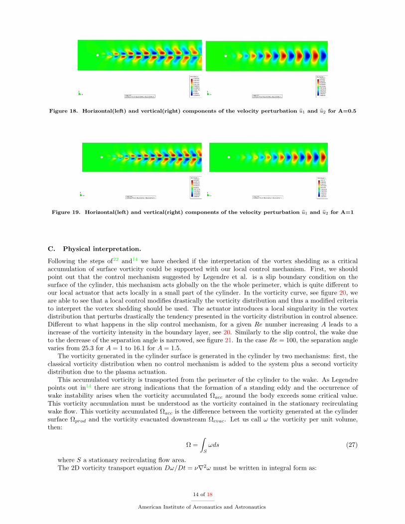
Figure 18. Horizontal(left) and vertical(right) components of the velocity perturbation u1 and u2 for A=0.5

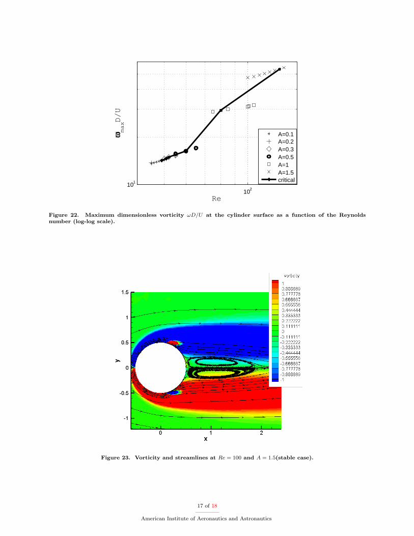
Figure 19. Horizontal(left) and vertical(right) components of the velocity perturbation u1 and u2 for A=1

C. Physical interpretation.

Following the steps of22 and14 we have checked if the interpretation of the vortex shedding as a criticalaccumulation of surface vorticity could be supported with our local control mechanism. First, we shouldpoint out that the control mechanism suggested by Legendre et al. is a slip boundary condition on thesurface of the cylinder, this mechanism acts globally on the the whole perimeter, which is quite different toour local actuator that acts locally in a small part of the cylinder. In the vorticity curve, see figure 20, weare able to see that a local control modifies drastically the vorticity distribution and thus a modified criteriato interpret the vortex shedding should be used. The actuator introduces a local singularity in the vortexdistribution that perturbs drastically the tendency presented in the vorticity distribution in control absence.Different to what happens in the slip control mechanism, for a given Re number increasing A leads to aincrease of the vorticity intensity in the boundary layer, see 20. Similarly to the slip control, the wake dueto the decrease of the separation angle is narrowed, see figure 21. In the case Re = 100, the separation anglevaries from 25.3 for A = 1 to 16.1 for A = 1.5.

The vorticity generated in the cylinder surface is generated in the cylinder by two mechanisms: first, theclassical vorticity distribution when no control mechanism is added to the system plus a second vorticitydistribution due to the plasma actuation.

This accumulated vorticity is transported from the perimeter of the cylinder to the wake. As Legendrepoints out in14 there are strong indications that the formation of a standing eddy and the occurrence ofwake instability arises when the vorticity accumulated Ωacc around the body exceeds some critical value.This vorticity accumulation must be understood as the vorticity contained in the stationary recirculatingwake flow. This vorticity accumulated Ωacc is the difference between the vorticity generated at the cylindersurface Ωprod and the vorticity evacuated downstream Ωevac. Let us call ω the vorticity per unit volume,then:

Ω =∫S

ωds (27)

where S a stationary recirculating flow area.The 2D vorticity transport equation Dω/Dt = ν∇2ω must be written in integral form as:

14 of 18


2 2.5 3−15

−10

−5

0

5

10

arc

Vor

ticity

A=0.1A=0.2A=0.3No actuation

Figure 20. Vorticity intensity at Re = 50 for the upper half of the cylinder, the arc parameter s ∈ [π/2, π]. Thedot green vertical line references the maximum control actuation.

Figure 21. Vorticity contour lines at Re = 100 at A = 0.5(top) and A = 1(bottom).

15 of 18


∫S

∂ω

∂tds+

∮L

ω(v · n)dl =∫S

ν∇2ωds (28)

where L is the closed material curve that limits the recirculation area S. Using also the Gauss theoremfor the viscous term, we have: ∫

S

∂ω

∂tds =

∮L

(ν∇ω · n− ωv · n) dl (29)

On the left hand side we have the accumulated vorticity in our recirculating flow area taking into accountthe viscous dissipation, on the other side we have the difference between the injected vorticity and theevacuated vorticity. This equation can be simplified as:

Ωacc = Ωprod − Ωevac (30)

According to Legendre when Ωacc exceeds a critical value the vortex shedding occurs. In the absence ofcontrol the accumulated vorticity can be related to the maximum value of the vorticity at the wall. Thecriterium that sustains that stability is related to the maximum accumulated vorticity can then be expressedin terms of a maximum value of vorticty at the wall. In our case, under forcing conditions the criterium basedon the maximum vorticity at the cylinder surface ωmax does not work so straight forward and it should bemodified. With our plasma control mechanism the vorticity distribution is far from being smooth as in theslip case and the singularity introduced by the actuator breaks the natural vorticity transport mechanism.The vorticity region that feeds the recirculation area is basically coming from the vorticity accumulatedin the body surface, when the plasma control is introduced a vorticity maximum appears in the cylindersurface. The presence of this local vorticity maximum in the cylinder surface prevents the natural transportmechanism from the production area to the wake area. The local maximum in the vorticity due to theactuator changes the sign of the vorticity gradient in a local area and consequently the natural transportmechanism. In this paper the maximum vorticity on the body surface criterium has been tested, see figure22, but the results obtained do not present such a concluding aspect as the ones presented by Legendre. Themaximum dimensionless vorticity results higher when the control parameter increases. Thus applying thecriterium of maximum vorticity at the wall and contrary to numerical simulation results and experimentsthe flow could not be stabilized when increasing actuation. Probably, and future works should point thisdirection, a more complex criterion inspired in the right hand side terms of the equation 29 should be defined.This means that with the plasma control used here, is not easy to define such criterion and the linear stabilityanalysis is the most appropriate tool to predict the vortex shedding.

It is worth mentioning that another big advantage of the linear stability analysis performed here is thatthe transition from two-dimensional flow to three dimensional flow can be easily studied by changing thevalue of the β = 2π/Lz parameter. In this work, in all flows close to the critical conditions, the β parameterhas been varied from β = [0, 10D] and no three-dimensional instability has been found. This result meansthat, different to the work performed by Legendre14 where the two-dimensionality of the flow was taken asan assumption, in this case the possible three-dimensional transition is taken into account in the analysisand no evidence was found.

VI. Conclusions.

In this work, we performed experimental and direct numerical simulations to study the influence of aplasma actuator on the dynamics of the two-dimensional wake behind a circular cylinder. The plasmaactuation takes place in a thin layer compared to cylinder diameter. This enables to subdivide the problemin two regions. A thin inner region where the forcing occurs and an outer region where electric forces canbe disregarded. A kinematic comptability condition has to be imposed at the boundary separating bothregions. We assume in our case that normal velocity is null and that no discontinuity in tangential velocitiesexists. No modelling of the inner region is proposed and the mathematical law that quantifies the tangentialvelocity distribution is determined from experiments. The presence of the plasma control delays the vortexshedding in the wake, makes the recirculation zone longer, alters the vorticity distribution on the cylinderand increases the shedding frequency. The critical control parameters where the vortex shedding is obtainedhas been studied as a function of the Reynolds number with a linear stability analysis of the Navier-Stokesequations. The derived generalized eigenvalue problem has been solved by an iterative Arnoldi method

16 of 18


102101

Re

ωmaxD/U

A=0.1A=0.2A=0.3A=0.5A=1A=1.5critical

Figure 22. Maximum dimensionless vorticity ωD/U at the cylinder surface as a function of the Reynoldsnumber (log-log scale).

Figure 23. Vorticity and streamlines at Re = 100 and A = 1.5(stable case).

17 of 18


and the critical modes, damping rates and frequencies of the dominant modes of the spectrum have beenobtained.

This three dimensional linear stability approach is also able to predict if the flow turns from 2D into a3D flow and we finally concluded that in our Reynolds number range no unstable 3D transition has beenfound. Therefore the presence of the actuator keeps the flow two-dimensional for all cylinder lengths.

The neutral stability curve that separates the stable region where no vortex shedding is present from theother periodic region has been calculated and a good agreement has been obtained with experiments.

Acknowledgments

We would like to acknowledge the financial support made available by the Universidad Politecnica deMadrid through the Mobility Research Programm UPM-2010. Leo M. Gonzalez wants to thank EusebioValero for the financial support to attend this Conference.

References

1Zielinska, B. and Wesfreid, J., “On the spatial structure of global modes in wake flow,” Physics of Fluids, Vol. 7, 1995,pp. 1418.

2Wesfreid, J., Goujon-Durand, S., and Zielinska, B., “Global mode behavior of the streamwise velocity in wakes.” Journalde Physique Paris II , Vol. 6, 1996., pp. 1343–1357.

3Moreau, E., “Airflow control by non thermal plasma actuators,” J. Phys. D: Appl. Phys., Vol. 40, 2007, pp. 605–36.4S. Masuda, M. W., “Ionic charging of very high resistivity spherical particle,” J. Electrostatics, Vol. 6, 1979, pp. 57–67.5Roth, J., Sherman, D., and Wilkinson, S., “Boundary layer flow control with a one atmosphere uniform glow discharge

surface plasma,” AIAA Meeting (Reno, USA, January 1998) paper #98-0328 , 1998.6Thomas, F., Koslov, A., and Corke, T., “Plasma actuators for bluff body flow control,” AIAA Meeting (San Francisco,

USA, June 2006) paper #2006-2845 , 2006.7Gonzalez, L. M., Artana, G., Gronskis, A., and D’Adamo, J., “A computational moving surface analogy of an electro-

dynamic control mechanism in bluff bodies,” Global Flow Instability and Flow Control IV, Crete, Greece, September 2009 ,2009.

8Gronskis, A., “Modelos numericos para el estudio de flujos externos controlados con actuadores EHD,” PhD Thesis. FIUBA, Jul 2009, pp. 1–293.

9Barkley, D., “Linear analysis of the cylinder wake mean flow,” Europhysics Letters, Vol. 75, No. 5, 2006, pp. 750–756.10Khor, M., Sheridan, J., Thompson, M., and Hourigan, K., “Global frequency selection in the observed time-mean wakes

of circular cylinders,” J. Fluid Mech, Vol. 601, 2008, pp. 425–441.11Leontini, J., Thompson, M., and Hourigan, K., “A numerical study of global frequency selection in the time-mean wake

of a circular cylinder,” J. Fluid Mech, Vol. 645, 2010, pp. 435–446.12Thiria, B. and Wesfreid, J., “Stability properties of forced wakes,” J. Fluid Mech, Vol. 579, 2007, pp. 137–161.13Thiria, B. and Wesfreid, J. E., “Physics of temporal forcing in wakes,” J Fluid Struct , Vol. 25, No. 4, Jun 2009, pp. 654–

665.14Legendre, D., Lauga, E., and Magnaudet, J., “Influence of slip on the dynamics of two-dimensional wakes,” J. Fluid

Mech, Vol. 633, (2009), pp. 437–447.15Moreau, E., “Airflow control by non-thermal plasma actuators.” J. Phys. D: Appl. Phys., Vol. 39 1, 2006, pp. 262.16E. Moreau, R. S. and Artana, G., “Electric wind produced by surface plasma actuators: a new dielectric barrier discharge

based on a three-electrode geometry.” J. Phys. D: Appl. Phys., Vol. 11, 2008, pp. 12pp.17Bermudez, M. M., Sosa, R., Grondona, D., Marquez, A., Kelly, H., and Artana, G., “Study of a pseudo-empirical model

approach to characterize plasma actuators,” Journal of Physics Conference Series, Vol. in press, 2010.18L.M., R. A. G., ADFC Navier-Stokes Solver , http://adfc.sourceforge.net/, 1999.19Theofilis, V., “Advances in global linear instability analysis of nonparallel and three-dimensional flows,” Prog. Aero. Sci.,

Vol. 39, 2003, pp. 249–315.20Gonzalez L, Theofilis V, and Gomez-Blanco R, “Finite-element numerical methods for viscous incompressible BiGlobal

linear instability analysis on unstructured meshes,” AIAA Journal , Vol. 45, No. 4, April 2007, pp. 840–855.21Barkley, D. and Henderson, R. D., “Three-dimensional Floquet stability analysis of the wake of a circular cylinder,”

Journal of Fluid Mechanics, Vol. 322, 1996, pp. 215–241.22Leal, L., “Vorticity transport and wake structure for bluff bodies at finite Reynolds number,” Phys. Fluids A 1 , 1989,

pp. 124–131.

18 of 18


Documents

The scenario of two-dimensional instabilities of the ... · actuators, dielectric barrier discharge (DBD) type. EHD actuators can add momentum to the ow around an object in regions