Embed Size (px)
Citation preview
Logical Methods in Computer ScienceVol. 5 (1:3) 2009, pp. 1–38www.lmcs-online.org
Submitted Apr. 22, 2008Published Feb. 19, 2009
THE SAFE LAMBDA CALCULUS
WILLIAM BLUM AND C.-H. LUKE ONG
Oxford University Computing Laboratory – School of Informatics, University of Edinburgh, UKe-mail address: [email protected]
Oxford University Computing Laboratory, Oxford, UKe-mail address: [email protected]
Abstract. Safety is a syntactic condition of higher-order grammars that constrains oc-currences of variables in the production rules according to their type-theoretic order. Inthis paper, we introduce the safe lambda calculus, which is obtained by transposing (andgeneralizing) the safety condition to the setting of the simply-typed lambda calculus. Incontrast to the original definition of safety, our calculus does not constrain types (to behomogeneous). We show that in the safe lambda calculus, there is no need to renamebound variables when performing substitution, as variable capture is guaranteed not tohappen. We also propose an adequate notion of β-reduction that preserves safety. In thesame vein as Schwichtenberg’s 1976 characterization of the simply-typed lambda calculus,we show that the numeric functions representable in the safe lambda calculus are exactlythe multivariate polynomials; thus conditional is not definable. We also give a characteri-zation of representable word functions. We then study the complexity of deciding beta-etaequality of two safe simply-typed terms and show that this problem is PSPACE-hard. Fi-nally we give a game-semantic analysis of safety: We show that safe terms are denoted byP-incrementally justified strategies. Consequently pointers in the game semantics of safeλ-terms are only necessary from order 4 onwards.
Introduction
Background. The safety condition was introduced by Knapik, Niwinski and Urzyczynat FoSSaCS 2002 [19] in a seminal study of the algorithmics of infinite trees generatedby higher-order grammars. The idea, however, goes back some twenty years to Damm[10] who introduced an essentially equivalent1 syntactic restriction (for generators of wordlanguages) in the form of derived types. A higher-order grammar (that is assumed to behomogeneously typed) is said to be safe if it obeys certain syntactic conditions that constrainthe occurrences of variables in the production (or rewrite) rules according to their type-theoretic order. Though the formal definition of safety is somewhat intricate, the condition
1998 ACM Subject Classification: F.3.2, F.4.1.Key words and phrases: lambda calculus, higher-order recursion scheme, safety restriction, game
semantics.Some of the results presented here were first published in TLCA proceedings [8].1See de Miranda’s thesis [12] for a proof.
LOGICAL METHODSl IN COMPUTER SCIENCE DOI:10.2168/LMCS-5 (1:3) 2009c© W. Blum and C.-H. L. OngCC© Creative Commons
2 W. BLUM AND C.-H. L. ONG
itself is manifestly important. As we survey in the following, higher-order safe grammarscapture fundamental structures in computation and offer clear algorithmic advantages:
• Word languages. Damm and Goerdt [11] have shown that the word languages generatedby order-n safe grammars form an infinite hierarchy as n varies over the natural numbers.The hierarchy gives an attractive classification of the semi-decidable languages: Levels 0,1 and 2 of the hierarchy are respectively the regular, context-free, and indexed languages(in the sense of Aho [5]), although little is known about higher orders.
Remarkably, for generating word languages, order-n safe grammars are equivalent toorder-n pushdown automata [11], which are in turn equivalent to order-n indexed gram-mars [24, 25].
• Trees. Knapik et al. have shown that the Monadic Second Order (MSO) theories of treesgenerated by safe (deterministic) grammars of every finite order are decidable2.
They have also generalized the equi-expressivity result due to Damm and Goerdt [11]to an equivalence result with respect to generating trees: A ranked tree is generated by anorder-n safe grammar if and only if it is generated by an order-n pushdown automaton.
• Graphs. Caucal [9] has shown that the MSO theories of graphs generated3 by safe gram-mars of every finite order are decidable. Recently Hague et al. have shown that the MSOtheories of graphs generated by order-n unsafe grammars are undecidable, but decidingtheir modal mu-calculus theories is n-EXPTIME complete [17].
Overview. In this paper, we examine the safety condition in the setting of the lambdacalculus. Our first task is to transpose it to the lambda calculus and express it as anappropriate sub-system of the simply-typed theory. A first version of the safe lambdacalculus has appeared in an unpublished technical report [4]. Here we propose a moregeneral and cleaner version where terms are no longer required to be homogeneously typed(see Section 1 for a definition). The formation rules of the calculus are designed to maintaina simple invariant: Variables that occur free in a safe λ-term have orders no smaller thanthat of the term itself. We can now explain the sense in which the safe lambda calculus is safeby establishing its salient property: No variable capture can ever occur when substitutinga safe term into another. In other words, in the safe lambda calculus, it is safe to usecapture-permitting substitution when performing β-reduction.
There is no need for new names when computing β-reductions of safe λ-terms, becauseone can safely “reuse” variable names in the input term. Safe lambda calculus is thuscheaper to compute in this naıve sense. Intuitively one would expect the safety constraintto lower the expressivity of the simply-typed lambda calculus. Our next contribution is togive a precise measure of the expressivity deficit of the safe lambda calculus. An old resultof Schwichtenberg [34] says that the numeric functions representable in the simply-typedlambda calculus are exactly the multivariate polynomials extended with the conditionalfunction. In the same vein, we show that the numeric functions representable in the safelambda calculus are exactly the multivariate polynomials.
2It has recently been shown [30] that trees generated by unsafe deterministic grammars (of every finiteorder) also have decidable MSO theories. More precisely, the MSO theory of trees generated by order-nrecursion schemes is n-EXPTIME complete.
3These are precisely the configuration graphs of higher-order pushdown systems.
THE SAFE LAMBDA CALCULUS 3
Our last contribution is to give a game-semantic account of the safe lambda calculus.Using a correspondence result relating the game semantics of a λ-term M to a set of tra-versals [30] over a certain abstract syntax tree of the η-long form of M (called computationtree), we show that safe terms are denoted by P-incrementally justified strategies. In sucha strategy, pointers emanating from the P-moves of a play are uniquely reconstructiblefrom the underlying sequence of moves and the pointers associated to the O-moves therein:Specifically, a P-question always points to the last pending O-question (in the P-view) of agreater order. Consequently pointers in the game semantics of safe λ-terms are only neces-sary from order 4 onwards. Finally we prove that a β-normal λ-term is safe if and only ifits strategy denotation is (innocent and) P-incrementally justified.
1. The safe lambda calculus
Higher-order safe grammars. We first present the safety restriction as it was originallydefined [19]. We consider simple types generated by the grammar A ::= o | A → A. Byconvention, → associates to the right. Thus every type can be written as A1 → · · · → An →o, which we shall abbreviate to (A1, · · · , An, o) (in case n = 0, we identify (o) with o). Wewill also use the notation An → B for every types A,B and positive natural number n > 0defined by induction as: A1 → B = A → B and An+1 → B = A → (An → B). The orderof a type is given by ord o = 0 and ord(A → B) = max(ordA + 1, ordB). We assume aninfinite set of typed variables. The order of a typed term or symbol is defined to be theorder of its type. The set of applicative terms over a set of typed symbols is defined as itsclosure under the application operation (i.e., if M : A → B and N : A are in the closurethen so does MN : B).
A (higher-order) grammar is a tuple 〈Σ,N ,R, S〉, where Σ is a ranked alphabet (inthe sense that each symbol f ∈ Σ is assumed to have type or → o where r is the arity off) of terminals; N is a finite set of typed non-terminals; S is a distinguished ground-typesymbol of N , called the start symbol; R is a finite set of production (or rewrite) rules, onefor each non-terminal F : (A1, . . . , An, o) ∈ N , of the form Fz1 . . . zm → e where each zi(called parameter) is a variable of type Ai and e is an applicative term of type o generatedfrom the typed symbols in Σ ∪ N ∪ {z1, . . . , zm}. We say that the grammar is order-n justin case the order of the highest-order non-terminal is n.
We call higher-order recursion scheme a higher-order grammar that is deterministic(i.e., for each non-terminal F ∈ N there is exactly one production rule with F on the lefthand side). Higher-order recursion schemes are used as generators of infinite trees. Thetree generated by a recursion scheme G is a possibly infinite applicative term, butviewed as a Σ-labelled tree; it is constructed from the terminals in Σ, and is obtained byunfolding the rewrite rules of G ad infinitum, replacing formal by actual parameters eachtime, starting from the start symbol S. See e.g. [19] for a formal definition.
g
a g
a h
h...
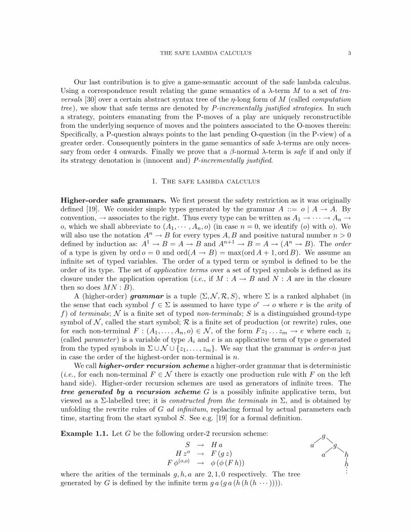
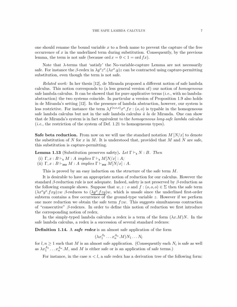
Example 1.1. Let G be the following order-2 recursion scheme:
S → H aH zo → F (g z)
F φ(o,o) → φ (φ (F h))
where the arities of the terminals g, h, a are 2, 1, 0 respectively. The treegenerated by G is defined by the infinite term g a (g a (h (h (h · · · )))).
4 W. BLUM AND C.-H. L. ONG
A type (A1, · · · , An, o) is said to be homogeneous if ordA1 ≥ ordA2 ≥ · · · ≥ ordAn,and each A1, . . . , An is homogeneous [19]. We reproduce the following Knapik et al.’sdefinition [19].
Definition 1.2 (Safe grammar). (All types are assumed to be homogeneous.) A term oforder k > 0 is unsafe if it contains an occurrence of a parameter of order strictly less than k,otherwise the term is safe. An occurrence of an unsafe term t as a subexpression of a termt′ is safe if it is in the context · · · (ts) · · · , otherwise the occurrence is unsafe. A grammaris safe if no unsafe term has an unsafe occurrence at a right-hand side of any production.
Example 1.3. (i) Take H : ((o, o), o) and f : (o, o, o); the following rewrite rules are unsafe(In each case we underline the unsafe subterm that occurs unsafely):
G(o,o) x → H (f x)
F ((o,o),o,o,o) z x y → f (F (F z y) y (z x))x
(ii) The order-2 grammar defined in Example 1.1 is unsafe.
Safety adapted to the lambda calculus. We assume a set Ξ of higher-order constants.We use sequents of the form Γ ⊢Ξ
$ M : A to represent term-in-context where Γ is the
context and A is the type of M . For convenience, we shall omit the superscript from ⊢Ξs
whenever the set of constants Ξ is clear from the context. The subscript in ⊢Ξ$ specifies
which type system is used to form the judgement: We use the subscript ‘st’ to refer to thetraditional system of rules of the Church-style simply-typed lambda calculus augmentedwith constants from Ξ. We will introduce a new subscripts for each type system that wedefine. For simplicity we write (A1, · · · , An, B) to mean A1 → · · · → An → B, where B isnot necessarily ground.
Definition 1.4. (i) The safe lambda calculus is a sub-system of the simply-typed lambdacalculus. It is defined as the set of judgements of the form Γ ⊢s M : A that are derivablefrom the following Church-style system of rules:
(var)x : A ⊢s x : A
(const)⊢s f : A
f ∈ Ξ (wk)Γ ⊢s M : A
∆ ⊢s M : AΓ ⊂ ∆
(appas)Γ ⊢asa M : A→ B Γ ⊢s N : A
Γ ⊢asa M N : B(δ)
Γ ⊢s M : A
Γ ⊢asa M : A
(app)Γ ⊢asa M : A→ B Γ ⊢s N : A
Γ ⊢s M N : BordB ≤ ordΓ
(abs)Γ, x1 : A1, . . . , xn : An ⊢asa M : B
Γ ⊢s λxA1
1 . . . xAnn .M : (A1, . . . , An, B)
ord(A1, . . . , An, B) ≤ ord Γ
where ord Γ denotes the set {ord y : y ∈ Γ} and “c ≤ S” means that c is a lower-bound ofthe set S. The subscripts in ⊢s and ⊢asa stand for “safe” and “almost safe application”.
(ii) The sub-system that is defined by the same rules in (i), such that all types thatoccur in them are homogeneous, is called the homogeneous safe lambda calculus.
(iii) We say that a term M is safe if the judgement Γ ⊢s M : T is derivable in the safelambda calculus for some context Γ and type T .
THE SAFE LAMBDA CALCULUS 5
The safe lambda calculus deviates from the standard definition of the simply-typedlambda calculus in a number of ways. First the rule (abs) can abstract several variablesat once. (Of course this feature alone does not alter expressivity.) Crucially, the sideconditions in the application rule and abstraction rule require the variables in the typingcontext to have orders no smaller than that of the term being formed. We do not imposeany constraint on types. In particular, type-homogeneity, which was an assumption of theoriginal definition of safe grammars [19], is not required here. Another difference is that weallow Ξ-constants to have arbitrary higher-order types.
Example 1.5 (Kierstead terms). Consider the terms M1 = λf ((o,o),o).f(λxo.f(λyo.y)) and
M2 = λf ((o,o),o).f(λxo.f(λyo.x)). The term M2 is not safe because in the subterm f(λyo.x),the free variable x has order 0 which is smaller than ord(λyo.x) = 1. On the other hand,M1 is safe.
It is easy to see that valid typing judgements of the safe lambda calculus satisfy thefollowing simple invariant:
Lemma 1.6. If Γ ⊢s M : A then every variable in Γ occurring free in M has order at leastordM .
Definition 1.7. A term is an almost safe applications if it is safe or if it is of the formN1 . . . Nm for some m ≥ 1 where N1 is not an application and for every 1 ≤ i ≤ m, Ni issafe.
A term is almost safe if either it is an almost safe application, or if it is of the formλxA1
1 . . . xAnn .M for n ≥ 1 and some almost safe application M .
An almost safe application is not necessarily safe but it can be used to form a safe termby applying sufficiently many safe terms to it. An almost safe term can be turned intoa safe term by either applying sufficiently many safe terms (if it is an application), or byabstracting sufficiently many variables (if it is an abstraction).
We have the following immediate lemma:
Lemma 1.8. A term M is
(i) an almost safe application iff there is a derivation of Γ ⊢asa M : T for some Γ, T ;
(ii) almost safe iff Γ ⊢asa M : T or if M ≡ λxA1
1 . . . xAnn .N and Γ ⊢asa N : T for some
Γ, T .
In particular, terms constructed with the rule (appas) are almost safe applications.
When restricted to the homogeneously-typed sub-system, the safe lambda calculus cap-tures the original notion of safety due to Knapik et al. in the context of higher-order gram-mars:
Proposition 1.9. Let G = 〈Σ,N ,R, S〉 be a grammar and let e be an applicative term
generated from the symbols in N ∪Σ∪{ zA1
1 , · · · , zAmm }. A rule Fz1 . . . zm → e in R is safe
(in the original sense of Knapik et al.) if and only if z1 : A1, · · · , zm : Am ⊢Σ∪Ns e : o is a
valid typing judgement of the homogeneous safe lambda calculus.
Proof. We show by induction that
6 W. BLUM AND C.-H. L. ONG
(i) z1, . . . , zm ⊢asa t : A is a valid judgement of the homogeneous safe lambda calculuscontaining no abstraction if and only if in the Knapik sense, all the occurrences of unsafesubterms of t are safe occurrences.
(ii) z1, . . . , zm ⊢s t : A is a valid judgement of the homogeneous safe lambda calculuscontaining no abstraction if and only if in the Knapik sense, all the occurrences of unsafesubterms of t are safe occurrences, and all parameters occurring in t have order greater thanord t.The constant and variable rule are trivial. Application case: By definition, a term t0 . . . tnis Knapik-safe iff for all 0 ≤ i ≤ n, all the occurrences of unsafe subterms of ti are safeoccurrences (in the Knapik sense), and for all 1 ≤ j ≤ n, the operands occurring in tjhave order greater than ord tj. The (appas) rule and the induction hypothesis permit us toconclude.
Now since e is an applicative term of ground type, the previous result gives: z1, . . . , zm ⊢s
e : o is a valid judgement of the homogeneous safe lambda calculus iff all the occurrencesof unsafe subterms of e are safe occurrences, which by definition of Knapik-safety is in turnequivalent to saying that the rule Fz1 . . . zm → e is safe.
In what sense is the safe lambda calculus safe? It is an elementary fact that when per-forming β-reduction in the lambda calculus, one must use capture-avoiding substitution,which is standardly implemented by renaming bound variables afresh upon each substi-tution. In the safe lambda calculus, however, variable capture can never happen (as thefollowing lemma shows). Substitution can therefore be implemented simply by capture-permitting replacement, without any need for variable renaming. In the following, we writeM{N/x} to denote the capture-permitting substitution4 of N for x in M .
Lemma 1.10 (No variable capture). There is no variable capture when performing capture-permitting substitution of N for x in M provided that Γ, x : B ⊢s M : A and Γ ⊢s N : B arevalid judgements of the safe lambda calculus.
Proof. We proceed by structural induction on M . The variable, constant and applicationcases are trivial. For the abstraction case, suppose M ≡ λy.R where y = y1 . . . yp. If x ∈ ythen M{N/x} = M and there is no variable capture.
Otherwise, x 6∈ y. By Lemma 1.8 R is of the form M1 . . .Mm for some m ≥ 1where M1 is not an application and for every 1 ≤ i ≤ m, Mi is safe. Thus we haveM{N/x} ≡ λy.M1{N/x} . . . Mm{N/x}. Let i ∈ {1..m}. By the induction hypothesis thereis no variable capture in Mi{N/x}. Thus variable capture can only happen if the follow-ing two conditions are met: (i) x occurs freely in Mi, (ii) some variable yi for 1 ≤ i ≤ poccurs freely in N . By Lemma 1.6, (ii) implies ord yi ≥ ordN = ordx and since x 6∈ y,condition (i) implies that x occurs freely in the safe term λy.R thus by Lemma 1.6 we haveordx ≥ ordλy.R ≥ 1 + ord yi > ord yi which gives a contradiction.
Remark 1.11. A version of the No-variable-capture Lemma also holds in safe grammars, asis implicit in (for example Lemma 3.2 of) the original paper [19].
Example 1.12. In order to contract the β-redex in the term
f : (o, o, o), x : o ⊢st (λϕ(o,o)xo.ϕ x)(f x) : (o, o)
4This substitution is done by textually replacing all free occurrences of x in M by N without performingvariable renaming. In particular for the abstraction case we have (λy1 . . . yn.M){N/x} = λy1 . . . yn.M{N/x}when x 6∈ {y1 . . . yn}.
THE SAFE LAMBDA CALCULUS 7
one should rename the bound variable x to a fresh name to prevent the capture of the freeoccurrence of x in the underlined term during substitution. Consequently, by the previouslemma, the term is not safe (because ordx = 0 < 1 = ord fx).
Note that λ-terms that ‘satisfy’ the No-variable-capture Lemma are not necessarilysafe. For instance the β-redex in λyozo.(λxo.y)z can be contracted using capture-permittingsubstitution, even though the term is not safe.
Related work: In her thesis [12], de Miranda proposed a different notion of safe lambdacalculus. This notion corresponds to (a less general version of) our notion of homogeneoussafe lambda calculus. It can be showed that for pure applicative terms (i.e., with no lambda-abstraction) the two systems coincide. In particular a version of Proposition 1.9 also holdsin de Miranda’s setting [12]. In the presence of lambda abstraction, however, our system is
less restrictive. For instance the term λf (o,o,o)xo.fx : (o, o) is typable in the homogeneoussafe lambda calculus but not in the safe lambda calculus a la de Miranda. One can showthat de Miranda’s system is in fact equivalent to the homogeneous long-safe lambda calculus(i.e., the restriction of the system of Def. 1.21 to homogeneous types).
Safe beta reduction. From now on we will use the standard notation M [N/x] to denotethe substitution of N for x in M . It is understood that, provided that M and N are safe,this substitution is capture-permitting.
Lemma 1.13 (Substitution preserves safety). Let Γ ⊢s N : B. Then
(i) Γ, x : B ⊢s M : A implies Γ ⊢s M [N/x] : A;(ii) Γ, x : B ⊢asa M : A implies Γ ⊢asa M [N/x] : A.
This is proved by an easy induction on the structure of the safe term M .
It is desirable to have an appropriate notion of reduction for our calculus. However thestandard β-reduction rule is not adequate. Indeed, safety is not preserved by β-reduction asthe following example shows. Suppose that w, z : o and f : (o, o, o) ∈ Σ then the safe term(λxoyo.fxy)zw β-reduces to (λyo.fzy)w, which is unsafe since the underlined first-ordersubterm contains a free occurrence of the ground-type variable z. However if we performone more reduction we obtain the safe term fzw. This suggests simultaneous contractionof “consecutive” β-redexes. In order to define this notion of reduction we first introducethe corresponding notion of redex.
In the simply-typed lambda calculus a redex is a term of the form (λx.M)N . In thesafe lambda calculus, a redex is a succession of several standard redexes:
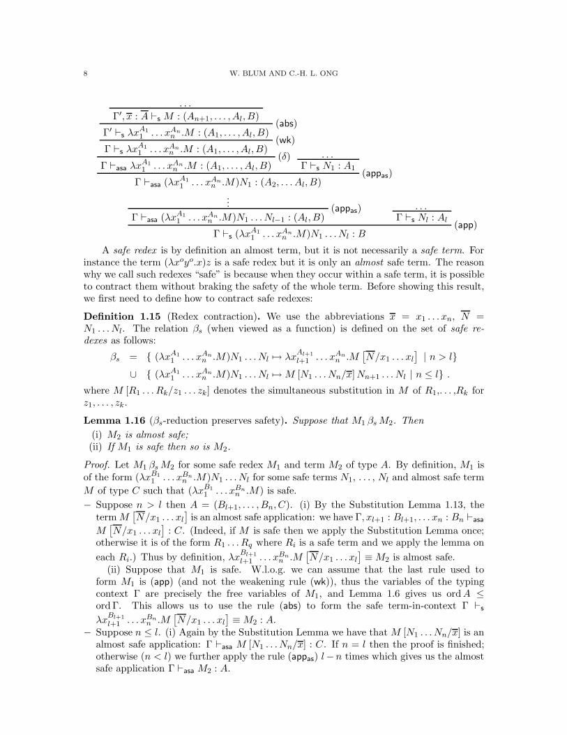
Definition 1.14. A safe redex is an almost safe application of the form
(λxA1
1 . . . xAnn .M)N1 . . . Nl
for l, n ≥ 1 such that M is an almost safe application. (Consequently each Ni is safe as well
as λxA1
1 . . . xAnn .M , and M is either safe or is an application of safe terms.)
For instance, in the case n < l, a safe redex has a derivation tree of the following form:
8 W. BLUM AND C.-H. L. ONG
. . .
Γ′, x : A ⊢s M : (An+1, . . . , Al, B)(abs)
Γ′ ⊢s λxA1
1 . . . xAnn .M : (A1, . . . , Al, B)
(wk)Γ ⊢s λx
A1
1 . . . xAnn .M : (A1, . . . , Al, B)
(δ)Γ ⊢asa λx
A1
1 . . . xAnn .M : (A1, . . . , Al, B)
. . .Γ ⊢s N1 : A1
(appas)Γ ⊢asa (λxA1
1 . . . xAnn .M)N1 : (A2, . . . Al, B)
... (appas)Γ ⊢asa (λxA1
1 . . . xAnn .M)N1 . . . Nl−1 : (Al, B)
. . .Γ ⊢s Nl : Al
(app)Γ ⊢s (λxA1
1 . . . xAnn .M)N1 . . . Nl : B
A safe redex is by definition an almost term, but it is not necessarily a safe term. Forinstance the term (λxoyo.x)z is a safe redex but it is only an almost safe term. The reasonwhy we call such redexes “safe” is because when they occur within a safe term, it is possibleto contract them without braking the safety of the whole term. Before showing this result,we first need to define how to contract safe redexes:
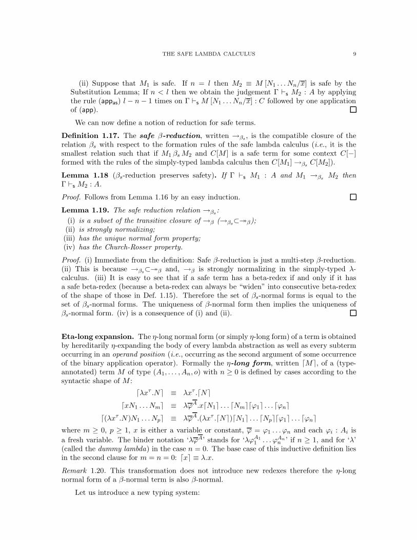
Definition 1.15 (Redex contraction). We use the abbreviations x = x1 . . . xn, N =N1 . . . Nl. The relation βs (when viewed as a function) is defined on the set of safe re-dexes as follows:
βs = { (λxA1
1 . . . xAnn .M)N1 . . . Nl 7→ λx
Al+1
l+1 . . . xAnn .M
[N/x1 . . . xl
]| n > l}
∪ { (λxA1
1 . . . xAnn .M)N1 . . . Nl 7→M [N1 . . . Nn/x]Nn+1 . . . Nl | n ≤ l} .
where M [R1 . . . Rk/z1 . . . zk] denotes the simultaneous substitution in M of R1,. . . ,Rk forz1, . . . , zk.
Lemma 1.16 (βs-reduction preserves safety). Suppose that M1 βsM2. Then
(i) M2 is almost safe;(ii) If M1 is safe then so is M2.
Proof. Let M1 βsM2 for some safe redex M1 and term M2 of type A. By definition, M1 isof the form (λxB1
1 . . . xBnn .M)N1 . . . Nl for some safe terms N1, . . . , Nl and almost safe term
M of type C such that (λxB1
1 . . . xBnn .M) is safe.
− Suppose n > l then A = (Bl+1, . . . , Bn, C). (i) By the Substitution Lemma 1.13, thetermM
[N/x1 . . . xl
]is an almost safe application: we have Γ, xl+1 : Bl+1, . . . xn : Bn ⊢asa
M[N/x1 . . . xl
]: C. (Indeed, if M is safe then we apply the Substitution Lemma once;
otherwise it is of the form R1 . . . Rq where Ri is a safe term and we apply the lemma on
each Ri.) Thus by definition, λxBl+1
l+1 . . . xBnn .M
[N/x1 . . . xl
]≡M2 is almost safe.
(ii) Suppose that M1 is safe. W.l.o.g. we can assume that the last rule used toform M1 is (app) (and not the weakening rule (wk)), thus the variables of the typingcontext Γ are precisely the free variables of M1, and Lemma 1.6 gives us ordA ≤ord Γ. This allows us to use the rule (abs) to form the safe term-in-context Γ ⊢s
λxBl+1
l+1 . . . xBnn .M
[N/x1 . . . xl
]≡M2 : A.
− Suppose n ≤ l. (i) Again by the Substitution Lemma we have that M [N1 . . . Nn/x] is analmost safe application: Γ ⊢asa M [N1 . . . Nn/x] : C. If n = l then the proof is finished;otherwise (n < l) we further apply the rule (appas) l−n times which gives us the almostsafe application Γ ⊢asa M2 : A.
THE SAFE LAMBDA CALCULUS 9
(ii) Suppose that M1 is safe. If n = l then M2 ≡ M [N1 . . . Nn/x] is safe by theSubstitution Lemma; If n < l then we obtain the judgement Γ ⊢s M2 : A by applyingthe rule (appas) l − n− 1 times on Γ ⊢s M [N1 . . . Nn/x] : C followed by one applicationof (app).
We can now define a notion of reduction for safe terms.
Definition 1.17. The safe β-reduction, written →βs, is the compatible closure of the
relation βs with respect to the formation rules of the safe lambda calculus (i.e., it is thesmallest relation such that if M1 βs M2 and C[M ] is a safe term for some context C[−]formed with the rules of the simply-typed lambda calculus then C[M1] →βs
C[M2]).
Lemma 1.18 (βs-reduction preserves safety). If Γ ⊢s M1 : A and M1 →βsM2 then
Γ ⊢s M2 : A.
Proof. Follows from Lemma 1.16 by an easy induction.
Lemma 1.19. The safe reduction relation →βs:
(i) is a subset of the transitive closure of →β (→βs⊂։β);
(ii) is strongly normalizing;(iii) has the unique normal form property;(iv) has the Church-Rosser property.
Proof. (i) Immediate from the definition: Safe β-reduction is just a multi-step β-reduction.(ii) This is because →βs
⊂։β and, →β is strongly normalizing in the simply-typed λ-calculus. (iii) It is easy to see that if a safe term has a beta-redex if and only if it hasa safe beta-redex (because a beta-redex can always be “widen” into consecutive beta-redexof the shape of those in Def. 1.15). Therefore the set of βs-normal forms is equal to theset of βs-normal forms. The uniqueness of β-normal form then implies the uniqueness ofβs-normal form. (iv) is a consequence of (i) and (ii).
Eta-long expansion. The η-long normal form (or simply η-long form) of a term is obtainedby hereditarily η-expanding the body of every lambda abstraction as well as every subtermoccurring in an operand position (i.e., occurring as the second argument of some occurrenceof the binary application operator). Formally the η-long form, written ⌈M⌉, of a (type-annotated) term M of type (A1, . . . , An, o) with n ≥ 0 is defined by cases according to thesyntactic shape of M :
⌈λxτ .N⌉ ≡ λxτ .⌈N⌉
⌈xN1 . . . Nm⌉ ≡ λϕA.x⌈N1⌉ . . . ⌈Nm⌉⌈ϕ1⌉ . . . ⌈ϕn⌉
⌈(λxτ .N)N1 . . . Np⌉ ≡ λϕA.(λxτ .⌈N⌉)⌈N1⌉ . . . ⌈Np⌉⌈ϕ1⌉ . . . ⌈ϕn⌉
where m ≥ 0, p ≥ 1, x is either a variable or constant, ϕ = ϕ1 . . . ϕn and each ϕi : Ai is
a fresh variable. The binder notation ‘λϕA’ stands for ‘λϕA1
1 . . . ϕAnn ’ if n ≥ 1, and for ‘λ’
(called the dummy lambda) in the case n = 0. The base case of this inductive definition liesin the second clause for m = n = 0: ⌈x⌉ ≡ λ.x.
Remark 1.20. This transformation does not introduce new redexes therefore the η-longnormal form of a β-normal term is also β-normal.
Let us introduce a new typing system:

10 W. BLUM AND C.-H. L. ONG
Definition 1.21. We define the set of long-safe terms by induction over the followingsystem of rules:
(varl)x : A ⊢l x : A
(constl)⊢l f : A
f ∈ Ξ (wkl)Γ ⊢l M : A
∆ ⊢l M : AΓ ⊂ ∆
(appl)Γ ⊢l M : (A1, . . . , An, B) Γ ⊢l N1 : A1 . . . Γ ⊢l Nn : An
Γ ⊢l MN1 . . . Nn : BordB ≤ ord Γ
(absl)Γ, x1 : A1, . . . , xn : An ⊢l M : B
Γ ⊢l λxA1
1 . . . xAnn .M : (A1, . . . , An, B)
ord(A1, . . . , An, B) ≤ ord Γ
The subscript in ⊢l stands for “long-safe”. This terminology is deliberately suggestiveof a forthcoming lemma. Note that long-safe terms are not necessarily in η-long normalform.
Observe that the system of rules from Def. 1.21 is a sub-system of the typing system ofDef. 1.4 where the application rule is restricted the same way as the abstraction rule (i.e.,it can perform multiple applications at once provided that all the variables in the contextof the resulting term have order greater than the order of the term itself). Thus we clearlyhave:
Lemma 1.22. If a term is long-safe then it is safe.
In general, long-safety is not preserved by η-expansion. For instance we have ⊢l λyozo.y :
(o, o, o) but performing one eta-expansion produces the term λxo.(λyozo.y)x : (o, o, o) whichis not long-safe. On the other hand, η-reduction (of one variable) preserves long-safety:
Lemma 1.23 (η-reduction of one variable preserves long-safety). Γ ⊢l λϕτ .M ϕ : A with ϕ
not occurring free in s implies Γ ⊢l M : A.
Proof. Suppose Γ ⊢l λϕτ .M ϕ : A. If M is an abstraction then by construction of M is
necessarily safe. If M ≡ N0 . . . Np with p ≥ 1 then again, since λϕτ .N0 . . . Npϕ is safe,each of the Ni is safe for 0 ≤ i ≤ p and for every variable z occurring free in λϕ.M ϕ,ord z ≥ ord(λϕτ .M ϕ) = ordM . Since ϕ does not occur free in M , the terms M andλϕτ .M ϕ have the same set of free variables, thus we can use the application rule to formΓ′ ⊢l N0 . . . Np : A where Γ′ consists of the typing-assignments for the free variables of M .The weakening rules permits us to conclude Γ ⊢l M : A.
Lemma 1.24 (η-long expansion preserves long-safety). Γ ⊢l M : A then Γ ⊢l ⌈M⌉ : A.
Proof. First we observe that for every variable or constant x : A we have x : A ⊢l ⌈x⌉ : A.We show this by induction on ordx. It is verified for every ground type variable x sincex = ⌈x⌉. Step case: x : A with A = (A1, . . . , An, o) and n > 0. Let ϕi : Ai be fresh variablesfor 1 ≤ i ≤ n. Since ordAi < ordx the induction hypothesis gives ϕi : Ai ⊢l ⌈ϕi⌉ : Ai.Using (wkl) we obtain x : A,ϕ : A ⊢l ⌈ϕi⌉ : Ai. The application rule gives x : A,ϕ : A ⊢l
x⌈ϕ1⌉ . . . ⌈ϕn⌉ : o and the abstraction rule gives x : A ⊢l λϕ.x⌈ϕ1⌉ . . . ⌈ϕn⌉ = ⌈x⌉ : A.We now prove the lemma by induction on M . The base case is covered by the previous
observation. Step case:
• M ≡ xN1 . . . Nm with x : (B1, . . . , Bm, A), A = (A1, . . . , An, o) for some m ≥ 0, n > 0and Ni : Bi for 1 ≤ i ≤ m. Let ϕi : Ai be fresh variables for 1 ≤ i ≤ n. By theprevious observation we have ϕi : Ai ⊢l ⌈ϕi⌉ : Ai, the weakening rule then gives us
THE SAFE LAMBDA CALCULUS 11
Γ, ϕ : A ⊢l ⌈ϕi⌉ : Ai. Since the judgement Γ ⊢l xN1 . . . Nm : A is formed using the(appl) rule, each Nj must be long-safe for 1 ≤ j ≤ m, thus by the induction hypothesis
we have Γ ⊢l ⌈Nj⌉ : Bj and by weakening we get Γ, ϕ : A ⊢l ⌈Nj⌉ : Bj. The (appl)
rule then gives Γ, ϕ : A ⊢l x⌈N1⌉ . . . ⌈Nm⌉⌈ϕ1⌉ . . . ⌈ϕn⌉ : o. Finally the (absl) rule givesΓ ⊢l λϕ.x⌈N1⌉ . . . ⌈Nm⌉⌈ϕ1⌉ . . . ⌈ϕn⌉ ≡ ⌈M⌉ : A, the side-condition of (absl) being verifiedsince ord ⌈s⌉ = ord s.
• M ≡ N0 . . . Nm where N0 is an abstraction and m ≥ 1. The eta-long normal form is⌈M⌉ ≡ λϕ.⌈N0⌉ . . . ⌈Nm⌉⌈ϕ1⌉ . . . ⌈ϕn⌉ for some fresh variables ϕ1, . . . , ϕn. Again, usingthe induction hypothesis we can easily derive Γ ⊢l ⌈M⌉ : A.
• M ≡ ληB.N where N of type C and is not an abstraction. The induction hypothesisgives Γ, η : B ⊢l ⌈N⌉ : C and using (absl) we get Γ ⊢l λη.⌈N⌉ ≡ ⌈M⌉ : A.
Remark 1.25.
(i) The converse of this lemma does not hold: performing η-reduction over a large ab-straction does not in general preserve long-safety. (This does not contradict Lemma1.23 which states that safety is preserved when performing η-reduction on an abstrac-tion of a single variable.) A counter-example is λf (o,o,o)g((o,o,o),o).g(λxo.fx), which is
not long-safe but whose eta-normal form λf (o,o,o)g((o,o,o),o).g(λxoyo.fxy) is long-safe.There are also closed terms in eta-normal form that are not long-safe but have anη-long normal form that is long-safe! Take for instance the closed βη-normal termλf (o,(o,o),o,o)g((o,o),o,o,o),o).g(λy(o,o)xo.fxy).
(ii) After performing η-long expansion of a term, all the occurrences of the application ruleare made long-safe. Thus if a term remains not long-safe after η-long expansion, thismeans that some variable occurrence is not bound by the first following application ofthe (abs) rule in the typing tree.
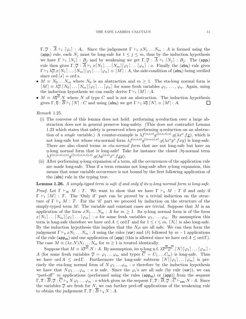
Lemma 1.26. A simply-typed term is safe if and only if its η-long normal form is long-safe.
Proof. Let Γ ⊢st M : T . We want to show that we have Γ ⊢s M : T if and only ifΓ ⊢l ⌈M⌉ : T . The ‘Only if’ part can be proved by a trivial induction on the struc-ture of Γ ⊢s M : T . For the ‘if’ part we proceed by induction on the structure of thesimply-typed term M : The variable and constant cases are trivial. Suppose that M is anapplication of the form xN1 . . . Nm : A for m ≥ 1. Its η-long normal form is of the formx⌈N1⌉ . . . ⌈Nm⌉⌈ϕ1⌉ . . . ⌈ϕm⌉ : o for some fresh variables ϕ1, . . .ϕm. By assumption thisterm is long-safe therefore we have ordA ≤ ordΓ and for 1 ≤ i ≤ m, ⌈Ni⌉ is also long-safe.By the induction hypothesis this implies that the Nis are all safe. We can then form thejudgement Γ ⊢s xN1 . . . Nm : A using the rules (var) and (δ) followed by m− 1 applicationsof the rule (appas) and one application of (app) (this is allowed since we have ordA ≤ ord Γ).The case M ≡ (λx.N)N1 . . . Nm for m ≥ 1 is treated identically.
Suppose thatM ≡ λxB.N : A. By assumption, its η-long n.f. λxBϕC .⌈N⌉⌈ϕ1⌉ . . . ⌈ϕm⌉ :A (for some fresh variables ϕ = ϕ1 . . . ϕm and types C = C1 . . . Cm) is long-safe. Thuswe have ordA ≤ ord Γ. Furthermore the long-safe subterm ⌈N⌉⌈ϕ1⌉ . . . ⌈ϕm⌉ is pre-cisely the eta-long normal form of N ϕ1 . . . ϕm : o therefore by the induction hypothesiswe have that Nϕ1 . . . ϕm : o is safe. Since the ϕi’s are all safe (by rule (var)), we can“peel-off” m applications (performed using the rules (appas) or (app)) from the sequentΓ, x : B,ϕ : C ⊢s N ϕ1 . . . ϕm : o which gives us the sequent Γ, x : B,ϕ : C ⊢asa N : A. Sincethe variables ϕ are fresh for N , we can further peel-off applications of the weakening ruleto obtain the judgement Γ, x : B ⊢s N : A.
12 W. BLUM AND C.-H. L. ONG
Finally since we have ordA ≤ ord Γ, we can use the rule (abs) to form the sequent
Γ ⊢s λxB .N : A.
Proposition 1.27. A term is safe if and only if its η-long normal form is safe.
Proof.
(If): Γ ⊢s ⌈M⌉ : T =⇒ Γ ⊢l ⌈M⌉ : T By Lemma 1.26 (only if),
=⇒ Γ ⊢s M : T By Lemma 1.26 (if).
(Only if): Γ ⊢s M : T =⇒ Γ ⊢l ⌈M⌉ : T By Lemma 1.26 (only if),
=⇒ Γ ⊢s ⌈M⌉ : T By Lemma 1.22.
The type inhabitation problem. It is well known that the simply-typed lambda cal-culus corresponds to intuitionistic implicative logic via the Curry-Howard isomorphism.The theorems of the logic correspond to inhabited types, and every inhabitant of a typerepresents a proof of the corresponding formula. Similarly, we can consider the fragmentof intuitionistic implicative logic that corresponds to the safe lambda calculus under theCurry-Howard isomorphism; we call it the safe fragment of intuitionistic implicative logic.
We would like to compare the reasoning power of these two logics, in other words, todetermine which types are inhabited in the lambda calculus but not in the safe lambdacalculus.5
If types are generated from a single atom o, then there is a positive answer: Everytype generated from one atom that is inhabited in the lambda calculus is also inhabited inthe safe lambda calculus. Indeed, one can transform any unsafe inhabitant M into a safeone of the same type as follows: Compute the eta-long beta normal form of M . Let x bean occurrence of a ground-type variable in a subterm of the form λx.C[x] where λx is thebinder of x and for some context C[−] different from the identity (defined as C[R] ≡ Rfor all R). We replace the subterm λx.C[x] by λx.x in M . This transformation is soundbecause both C[x] and x are of the same ground type. We repeat this procedure untilthe term stabilizes. This procedure clearly terminates since the size of the term decreasesstrictly after each step. The final term obtained is safe and of the same type as M .
This argument cannot be generalized to types generated from multiple atoms. Infact there are order-3 types with only 2 atoms that are inhabited in the simply-typedlambda calculus but not in the safe lambda calculus. Take for instance the order-3 type(((b, a), b), ((a, b), a), a) for some distinct atoms a and b. It is only inhabited by the followingfamily of terms which are all unsafe:
λf ((b,a),b)g((a,b),a).g(λxa1.f(λyb
1.x1))
λf ((b,a),b)g((a,b),a).g(λxa1.f(λyb
1.g(λxa2 .y1)))
λf ((b,a),b)g((a,b),a).g(λxa1.f(λyb
1.g(λxa2 .f(λyb
2.xi))) where i = 1, 2
λf ((b,a),b)g((a,b),a).g(λxa1.f(λyb
1.g(λxa2 .f(λyb
2.g(λxa3 .yi))) where i = 1, 2
. . .
5This problem was raised to our attention by Ugo dal Lago.
THE SAFE LAMBDA CALCULUS 13
Another example is the type of function composition. For any atom a and naturalnumber n ∈ N, we define the types na as follows: 0a = a and (n + 1)a = na → a. Takethree distinct atoms a, b and c. For any i, j, k ∈ N, we write σ(i, j, k) to denote the type
σ(i, j, k) ≡ (ia → jb) → (jb → kc) → ia → kc .
For all i, j, k, this type is inhabited in the lambda calculus by the “function compositionterm”:
λxyz.y(x z) .
This term is safe if and only if i ≥ j (for the subterm x z is safe iff i = ord(ia) = ord z ≥ord(x z) = ord(jb) = j). In the case i < j, the type σ(i, j, k) may still be safely inhabited.For instance σ(1, 3, 4) is inhabited by the safe term
λx1a→3by3b→4cz1c .y(x(λua.u)) .
The order-4 type σ(0, 2, 0), however, is only inhabited by the unsafe term λxyz.y(xz).Statman showed [35] that the problem of deciding whether a type defined over an
infinite number of ground atoms is inhabited (or equivalently of deciding validity of anintuitionistic implicative formula) is PSPACE-complete. The previous observations suggestthat the validity problem for the safe fragment of implicative logic may not be PSPACE-hard.
2. Expressivity
2.1. Numeric functions representable in the safe lambda calculus. Natural num-bers can be encoded in the simply-typed lambda calculus using the Church Numerals: eachn ∈ N is encoded as the term n = λs(o,o)zo.snz of type I = ((o, o), o, o) where o is a groundtype. We say that a p-ary function f : N
p → N, for p ≥ 0, is represented by a termF : (I, . . . , I, I) (with p+ 1 occurrences of I) if for all mi ∈ N, 0 ≤ i ≤ p we have:
F m1 . . .mp =β f(m1, . . . ,mp) .
Schwichtenberg [34] showed the following:
Theorem 2.1 (Schwichtenberg, 1976). The numeric functions representable by simply-typed lambda-terms of type I → . . . → I using the Church Numeral encoding are exactly themultivariate polynomials extended with the conditional function.
If we restrict ourselves to safe terms, the representable functions are exactly the multi-variate polynomials:
Theorem 2.2. The functions representable by safe lambda-expressions of type I → . . . → Iare exactly the multivariate polynomials.
Proof. Natural numbers are encoded as the Church Numerals: n = λsz.snz for eachn ∈ N. Addition: For n,m ∈ N, n+m = λα(o,o)xo.(nα)(mαx). Multiplication: n.m =
λα(o,o).n(mα). These terms are all safe, furthermore function composition can be safely en-coded: take a function g : N
n → N represented by safe term G of type In → I and functionsf1, . . . , fn : N
p → N represented by safe terms F1, . . . Fn respectively then the composedfunction (x1, · · · , xp) 7→ g(f1(x1, . . . , xp), . . . , fn(x1, . . . , xp)) is represented by the safe termλc1 . . . cp.G(F1c1 . . . cp) . . . (Fnc1 . . . cp). Hence any multivariate polynomial P (n1, . . . , nk)can be computed by composing the addition and multiplication terms as appropriate.
14 W. BLUM AND C.-H. L. ONG
For the converse, let U be a safe lambda-term of type I → I → I. The generalizationto terms of type In → I for every n ∈ N is immediate (they correspond to polynomials withn variables). By Lemma 1.27, safety is preserved by η-long normal expansion therefore wecan assume that U is in η-long normal form.
Let N τΣ denote the set of safe η-long β-normal terms of type τ with free variables in
Σ, and AτΣ for the set of β-normal terms of type τ with free variables in Σ and of the
form ϕs1 . . . sm for some variable ϕ : (A1, . . . , Am, o) where m ≥ 0 and for all 1 ≤ i ≤ m,
si ∈ NAi
Σ . Observe that the set AoΣ contains only safe terms but the sets Aτ
Σ in general maycontain unsafe terms. Let Σ denote the alphabet {x, y : I, z : o, α : o → o}. By an easyreasoning (See the term grammar construction of Zaionc [37]), we can derive the followingequations inducing a grammar over the set of terminals Σ ∪ {λxyαz., λz.} that generates
precisely the terms of N(I,I,I)∅ :
N(I,I,I)∅ → λxyαz.Ao
Σ
AoΣ → z | A
(o,o)Σ Ao
Σ
A(o,o)Σ → α | AI
Σ N(o,o)Σ
N(o,o)Σ → λz.Ao
Σ
AIΣ → x | y .
The key rule is the fourth one: had we not imposed the safety constraint the right-hand side
would instead be of the form λwo.A(o,o)Σ∪{w:o}. Here the safety constraint imposes to abstract
all the ground type variables occurring freely, thus only one free variable of ground typecan appear in the term and we can choose it to be named z up to α-conversion.
We extend the notion of representability to terms of type o, (o, o) and I with freevariables in Σ as follows: A function f : N
2 → N is represented by (i) Σ ⊢st F : o if and
only if for all m,n ∈ N, F [m,n/x, y] =β αf(m,n)z; (ii) Σ ⊢st G : (o, o) iff G[m,n/x, y] =β
λz.αf(m,n)z; (iii) Σ ⊢st H : I iff H[m,n/x, y] =β λαz.αf(m,n)z.
We now show by induction on the grammar rules that any term generated by thegrammar represents some polynomial: Base case: The term x and y represent the projectionfunctions (m,n) 7→ m and (m,n) 7→ n respectively. The term α and z represent the constantfunctions (m,n) 7→ 1 and (m,n) 7→ 0 respectively. Step case: The first and fourth rule aretrivial: for F ∈ Ao
Σ, the terms λz.F and λxyαz.F represent the same function as F . Wenow consider the second and third rule. We observe that for m, p, p′ ≥ 0 we have
(i) m (λz.αpz) =β λz.αm·pz; (ii) (λz.αpz)(αp′z) =β α
p+p′z .
Suppose that F ∈ AIΣ and G ∈ N
(o,o)Σ represent the functions f and g respectively then
by (i), FG represents the function f × g. If F ∈ A(o,o)Σ and G ∈ N o
Σ represent the functionsf and g then by (ii), FG represents the function f + g.
Hence U represents some polynomial: for all m,n ∈ N we have U m n =β λαz.αp(m,n)z
where p(m,n) =∑
0≤k≤dmiknjk for some ik, jk ≥ 0, d ≥ 0.
Corollary 2.3. The conditional operator C : I → I → I → I satisfying:
C t y z →β
{y, if t→β 0 ;z, if t→β n+ 1 .
is not definable in the simply-typed safe lambda calculus.
THE SAFE LAMBDA CALCULUS 15
Example 2.4. The term λFGHαx.F (λy.Gαx)(Hαx) used by Schwichtenberg [34] to definethe conditional operator is unsafe since the underlined subterm, which is of order 1, occursat an operand position and contains an occurrence of x of order 0.
Remark 2.5.
(i) This corollary tells us that the conditional function is not definable when numbers arerepresented by the Church Numerals. It may still be possible, however, to representthe conditional function using a different encoding for natural numbers. One way tocompensate for the loss of expressivity caused by the safety constraint is to introducecountably many domains of representation for natural numbers. Such a technique isused to represent the predecessor function in the simply-typed lambda calculus [14].
(ii) The boolean conditional can be represented in the safe lambda calculus as follows:We encode booleans by terms of type B = (o, o, o). The two truth values are thenrepresented by λxoyo.x and λxoyo.y and the conditional operator is given by the termλFBGBHBxoyo.F (Gxy)(H xy).
(iii) It is also possible to define a conditional operator behaving like the conditional operatorC in the second-order lambda calculus [14]: natural numbers are represented by termsn ≡ Λt.λst→tzt.sn(z) of type J ≡ ∆t.(t→ t) → (t→ t) and the conditional is encodedby the term λF JGJHJ .F J (λuJ .G) H. Whether this term is safe or not cannot beanswered just yet as we do not have a notion of safety for second-order typed terms.
2.2. Word functions definable in the safe lambda calculus. Schwichtenberg’s resulton numeric functions definable in the lambda calculus was extended to richer structures:Zaionc studied the problem for word functions, then functions over trees and eventually thegeneral case of functions over free algebras [20, 39, 38, 37, 40]. In this section we considerthe case of word functions expressible in the safe lambda calculus.
Word functions. We consider a binary alphabet Σ = {a, b}. The result of this sectionnaturally extends to all finite alphabets. We consider the set Σ∗ of all words over Σ. Theempty words is denoted ǫ. We write |w| to denote the length of the word w ∈ Σ∗. For anyk ∈ N we write k to denote the word a . . . a with k occurrences of a, so that |k| = k. Forany n ≥ 1 and k ≥ 0, we write c(n, k) for the n-ary function (Σ∗)n → Σ∗ that maps allinputs to the word k. We consider various word functions. Let x, y, z be words over Σ:
• Concatenation app : (Σ∗)2 → Σ∗. The word app(x, y) is the concatenation of x and y.• Substitution sub : (Σ∗)3 → Σ∗. The word sub(x, y, z) is obtained from x by substituting
the word y for all occurrences of a and z for all occurrences of b. Formally:
sub(ǫ, y, z) = ǫ ,
sub(ax, y, z) = app(y, sub(x, y, z)) ,
sub(bx, y, z) = app(z, sub(x, y, z)) .
• Prefix-cut cuta : Σ∗ → Σ∗. The word cuta x is the maximal prefix of x containing onlythe letter ’a’. Formally:
cuta(ǫ) = ǫ ,
cuta(ax) = app(a, cuta(x)) ,
cuta(bx) = ǫ .
16 W. BLUM AND C.-H. L. ONG
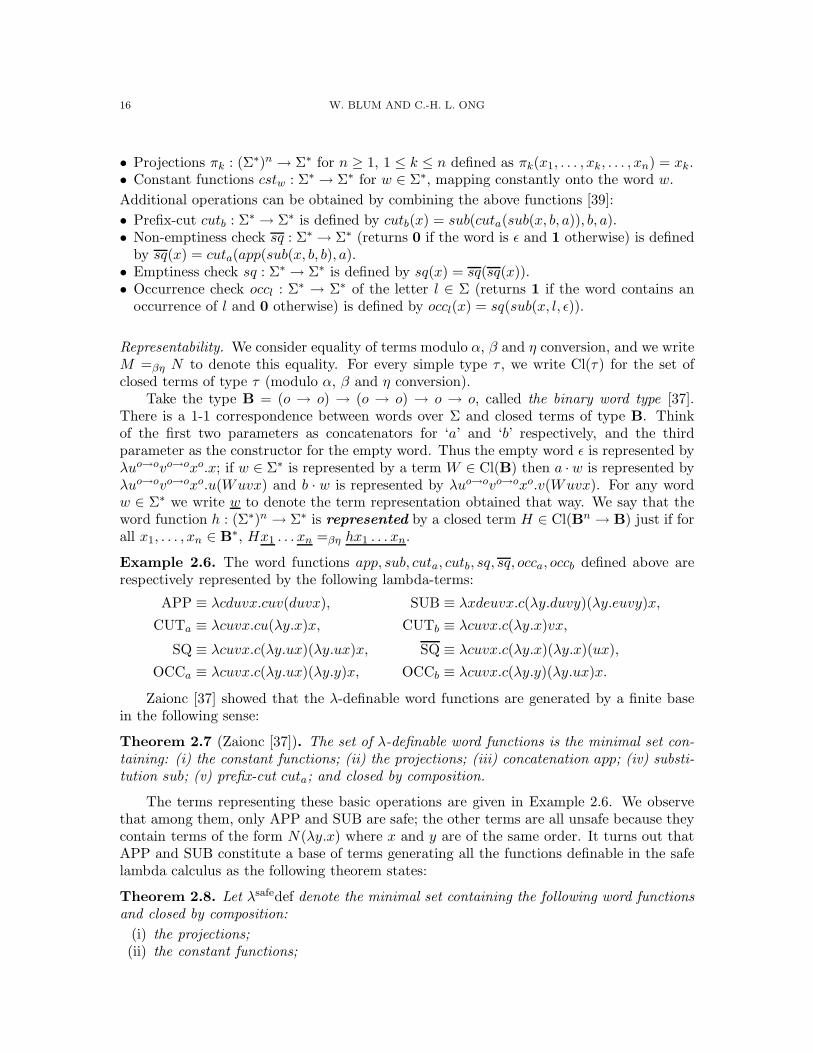
• Projections πk : (Σ∗)n → Σ∗ for n ≥ 1, 1 ≤ k ≤ n defined as πk(x1, . . . , xk, . . . , xn) = xk.• Constant functions cstw : Σ∗ → Σ∗ for w ∈ Σ∗, mapping constantly onto the word w.
Additional operations can be obtained by combining the above functions [39]:
• Prefix-cut cutb : Σ∗ → Σ∗ is defined by cutb(x) = sub(cuta(sub(x, b, a)), b, a).• Non-emptiness check sq : Σ∗ → Σ∗ (returns 0 if the word is ǫ and 1 otherwise) is defined
by sq(x) = cuta(app(sub(x, b, b), a).• Emptiness check sq : Σ∗ → Σ∗ is defined by sq(x) = sq(sq(x)).• Occurrence check occl : Σ∗ → Σ∗ of the letter l ∈ Σ (returns 1 if the word contains an
occurrence of l and 0 otherwise) is defined by occl(x) = sq(sub(x, l, ǫ)).
Representability. We consider equality of terms modulo α, β and η conversion, and we writeM =βη N to denote this equality. For every simple type τ , we write Cl(τ) for the set ofclosed terms of type τ (modulo α, β and η conversion).
Take the type B = (o → o) → (o → o) → o → o, called the binary word type [37].There is a 1-1 correspondence between words over Σ and closed terms of type B. Thinkof the first two parameters as concatenators for ‘a’ and ‘b’ respectively, and the thirdparameter as the constructor for the empty word. Thus the empty word ǫ is represented byλuo→ovo→oxo.x; if w ∈ Σ∗ is represented by a term W ∈ Cl(B) then a ·w is represented byλuo→ovo→oxo.u(Wuvx) and b · w is represented by λuo→ovo→oxo.v(Wuvx). For any wordw ∈ Σ∗ we write w to denote the term representation obtained that way. We say that theword function h : (Σ∗)n → Σ∗ is represented by a closed term H ∈ Cl(Bn → B) just if forall x1, . . . , xn ∈ B∗, Hx1 . . . xn =βη hx1 . . . xn.
Example 2.6. The word functions app, sub, cuta, cutb, sq, sq, occa, occb defined above arerespectively represented by the following lambda-terms:
APP ≡ λcduvx.cuv(duvx), SUB ≡ λxdeuvx.c(λy.duvy)(λy.euvy)x,
CUTa ≡ λcuvx.cu(λy.x)x, CUTb ≡ λcuvx.c(λy.x)vx,
SQ ≡ λcuvx.c(λy.ux)(λy.ux)x, SQ ≡ λcuvx.c(λy.x)(λy.x)(ux),
OCCa ≡ λcuvx.c(λy.ux)(λy.y)x, OCCb ≡ λcuvx.c(λy.y)(λy.ux)x.
Zaionc [37] showed that the λ-definable word functions are generated by a finite basein the following sense:
Theorem 2.7 (Zaionc [37]). The set of λ-definable word functions is the minimal set con-taining: (i) the constant functions; (ii) the projections; (iii) concatenation app; (iv) substi-tution sub; (v) prefix-cut cuta; and closed by composition.
The terms representing these basic operations are given in Example 2.6. We observethat among them, only APP and SUB are safe; the other terms are all unsafe because theycontain terms of the form N(λy.x) where x and y are of the same order. It turns out thatAPP and SUB constitute a base of terms generating all the functions definable in the safelambda calculus as the following theorem states:
Theorem 2.8. Let λsafedef denote the minimal set containing the following word functionsand closed by composition:
(i) the projections;(ii) the constant functions;
THE SAFE LAMBDA CALCULUS 17
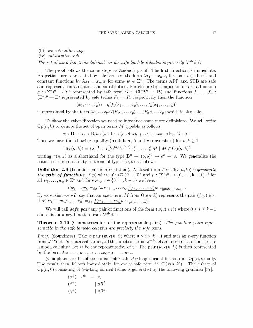
(iii) concatenation app;(iv) substitution sub.
The set of word functions definable in the safe lambda calculus is precisely λsafedef.
The proof follows the same steps as Zaionc’s proof. The first direction is immediate:Projections are represented by safe terms of the form λx1 . . . xn.xi for some i ∈ {1..n}, andconstant functions by λx1 . . . xn.w for some w ∈ Σ∗. The terms APP and SUB are safeand represent concatenation and substitution. For closure by composition: take a functiong : (Σ∗)n → Σ∗ represented by safe term G ∈ Cl(Bn → B) and functions f1, . . . , fn :(Σ∗)p → Σ∗ represented by safe terms F1, . . . Fn respectively then the function
(x1, · · · , xp) 7→ g(f1(x1, . . . , xp), . . . , fn(x1, . . . , xp))
is represented by the term λc1 . . . cp.G(F1c1 . . . cp) . . . (Fnc1 . . . cp) which is also safe.
To show the other direction we need to introduce some more definitions. We will writeOp(n, k) to denote the set of open terms M typable as follows:
c1 : B, . . . cn : B, u : (o, o), v : (o, o), xk−1 : o, . . . , x0 : o ⊢st M : o .
Thus we have the following equality (modulo α, β and η conversions) for n, k ≥ 1:
Cl(τ(n, k)) = {λcB1 . . . cB
n u(o,o)v(o,o)xo
k−1 . . . xo0.M | M ∈ Op(n, k)}
writing τ(n, k) as a shorthand for the type Bn → (o, o)2 → ok → o. We generalize thenotion of representability to terms of type τ(n, k) as follows:
Definition 2.9 (Function pair representation). A closed term T ∈ Cl(τ(n, k)) represents
the pair of functions (f, p) where f : (Σ∗)n → Σ∗ and p : (Σ∗)n → {0, . . . ,k − 1} if forall w1, . . . , wn ∈ Σ∗ and for every i ∈ {0 . . . , k − 1} we have:
Tw1 . . . wn =βη λuvxk−1 . . . x0.f(w1, . . . , wn)uvx|p(w1,...,wn)| .
By extension we will say that an open term M from Op(n, k) represents the pair (f, p) justif M [w1 . . . wn/c1 . . . cn] =βη f(w1, . . . , wn)uvx|p(w1,...,wn)|.
We will call safe pair any pair of functions of the form (w, c(n, i)) where 0 ≤ i ≤ k− 1and w is an n-ary function from λsafedef.
Theorem 2.10 (Characterization of the representable pairs). The function pairs repre-sentable in the safe lambda calculus are precisely the safe pairs.
Proof. (Soundness). Take a pair (w, c(n, i)) where 0 ≤ i ≤ k− 1 and w is an n-ary functionfrom λsafedef. As observed earlier, all the functions from λsafedef are representable in the safelambda calculus: Let w be the representative of w. The pair (w, c(n, i)) is then representedby the term λc1 . . . cnuvxk−1 . . . x0.wc1 . . . cnuvxi.
(Completeness) It suffices to consider safe β-η-long normal terms from Op(n, k) only.The result then follows immediately for every safe term in Cl(τ(n, k)). The subset ofOp(n, k) consisting of β-η-long normal terms is generated by the following grammar [37]:
(αki ) Rk → xi
(βk) | uRk
(γk) | vRk
18 W. BLUM AND C.-H. L. ONG
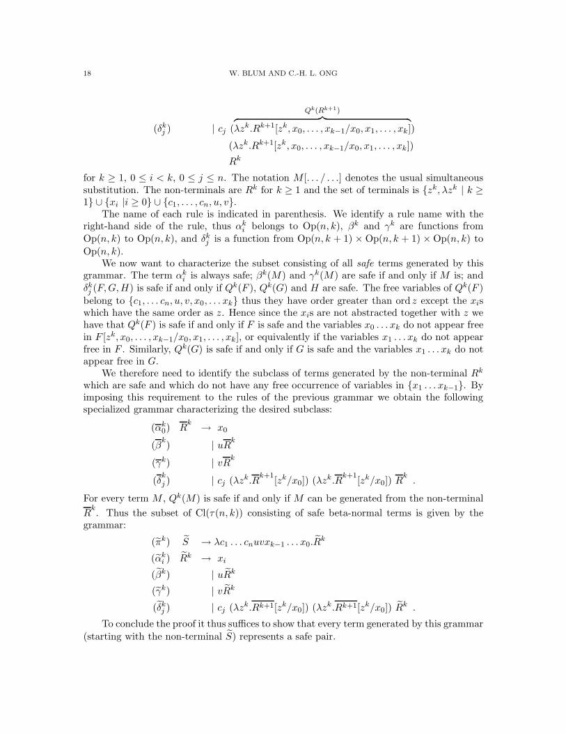
(δkj ) | cj (
Qk(Rk+1)︷ ︸︸ ︷λzk.Rk+1[zk, x0, . . . , xk−1/x0, x1, . . . , xk])
(λzk.Rk+1[zk, x0, . . . , xk−1/x0, x1, . . . , xk])
Rk
for k ≥ 1, 0 ≤ i < k, 0 ≤ j ≤ n. The notation M [. . . / . . .] denotes the usual simultaneoussubstitution. The non-terminals are Rk for k ≥ 1 and the set of terminals is {zk, λzk | k ≥1} ∪ {xi |i ≥ 0} ∪ {c1, . . . , cn, u, v}.
The name of each rule is indicated in parenthesis. We identify a rule name with theright-hand side of the rule, thus αk
i belongs to Op(n, k), βk and γk are functions fromOp(n, k) to Op(n, k), and δk
j is a function from Op(n, k + 1) × Op(n, k + 1) × Op(n, k) to
Op(n, k).We now want to characterize the subset consisting of all safe terms generated by this
grammar. The term αki is always safe; βk(M) and γk(M) are safe if and only if M is; and
δkj (F,G,H) is safe if and only if Qk(F ), Qk(G) and H are safe. The free variables of Qk(F )
belong to {c1, . . . cn, u, v, x0, . . . xk} thus they have order greater than ord z except the xiswhich have the same order as z. Hence since the xis are not abstracted together with z wehave that Qk(F ) is safe if and only if F is safe and the variables x0 . . . xk do not appear freein F [zk, x0, . . . , xk−1/x0, x1, . . . , xk], or equivalently if the variables x1 . . . xk do not appearfree in F . Similarly, Qk(G) is safe if and only if G is safe and the variables x1 . . . xk do notappear free in G.
We therefore need to identify the subclass of terms generated by the non-terminal Rk
which are safe and which do not have any free occurrence of variables in {x1 . . . xk−1}. Byimposing this requirement to the rules of the previous grammar we obtain the followingspecialized grammar characterizing the desired subclass:
(αk0) R
k→ x0
(βk) | uR
k
(γk) | vRk
(δk
j ) | cj (λzk.Rk+1
[zk/x0]) (λzk.Rk+1
[zk/x0]) Rk.
For every term M , Qk(M) is safe if and only if M can be generated from the non-terminal
Rk. Thus the subset of Cl(τ(n, k)) consisting of safe beta-normal terms is given by the
grammar:
(πk) S → λc1 . . . cnuvxk−1 . . . x0.Rk
(αki ) Rk → xi
(βk) | uRk
(γk) | vRk
(δkj ) | cj (λzk.Rk+1[zk/x0]) (λzk.Rk+1[zk/x0]) R
k .
To conclude the proof it thus suffices to show that every term generated by this grammar
(starting with the non-terminal S) represents a safe pair.
THE SAFE LAMBDA CALCULUS 19
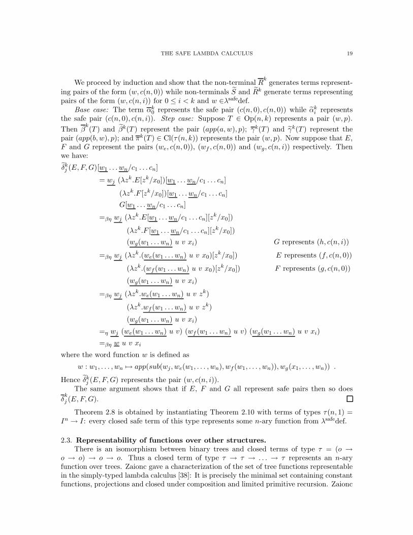
We proceed by induction and show that the non-terminal Rk
generates terms represent-
ing pairs of the form (w, c(n, 0)) while non-terminals S and Rk generate terms representingpairs of the form (w, c(n, i)) for 0 ≤ i < k and w ∈λsafedef.
Base case: The term αk0 represents the safe pair (c(n, 0), c(n, 0)) while αk
i representsthe safe pair (c(n, 0), c(n, i)). Step case: Suppose T ∈ Op(n, k) represents a pair (w, p).
Then βk(T ) and βk(T ) represent the pair (app(a,w), p); γk(T ) and γk(T ) represent the
pair (app(b, w), p); and πk(T ) ∈ Cl(τ(n, k)) represents the pair (w, p). Now suppose that E,F and G represent the pairs (we, c(n, 0)), (wf , c(n, 0)) and (wg, c(n, i)) respectively. Thenwe have:
δkj (E,F,G)[w1 . . . wn/c1 . . . cn]
= wj (λzk.E[zk/x0])[w1 . . . wn/c1 . . . cn]
(λzk.F [zk/x0])[w1 . . . wn/c1 . . . cn]
G[w1 . . . wn/c1 . . . cn]
=βη wj (λzk.E[w1 . . . wn/c1 . . . cn][zk/x0])
(λzk.F [w1 . . . wn/c1 . . . cn][zk/x0])
(wg(w1 . . . wn) u v xi) G represents (h, c(n, i))
=βη wj (λzk.(we(w1 . . . wn) u v x0)[zk/x0]) E represents (f, c(n, 0))
(λzk.(wf (w1 . . . wn) u v x0)[zk/x0]) F represents (g, c(n, 0))
(wg(w1 . . . wn) u v xi)
=βη wj (λzk.we(w1 . . . wn) u v zk)
(λzk.wf (w1 . . . wn) u v zk)
(wg(w1 . . . wn) u v xi)
=η wj (we(w1 . . . wn) u v) (wf (w1 . . . wn) u v) (wg(w1 . . . wn) u v xi)
=βη w u v xi
where the word function w is defined as
w : w1, . . . , wn 7→ app(sub(wj , we(w1, . . . , wn), wf (w1, . . . , wn)), wg(x1, . . . , wn)) .
Hence δkj (E,F,G) represents the pair (w, c(n, i)).
The same argument shows that if E, F and G all represent safe pairs then so does
δkj (E,F,G).
Theorem 2.8 is obtained by instantiating Theorem 2.10 with terms of types τ(n, 1) =In → I: every closed safe term of this type represents some n-ary function from λsafedef.
2.3. Representability of functions over other structures.
There is an isomorphism between binary trees and closed terms of type τ = (o →o → o) → o → o. Thus a closed term of type τ → τ → . . . → τ represents an n-aryfunction over trees. Zaionc gave a characterization of the set of tree functions representablein the simply-typed lambda calculus [38]: It is precisely the minimal set containing constantfunctions, projections and closed under composition and limited primitive recursion. Zaionc
20 W. BLUM AND C.-H. L. ONG
showed that the same characterization holds for the general case of functions expressed over(different) free algebras [39, 40] (they are again given by the minimal set containing constantfunctions, projections and closed under composition and limited primitive recursion). Thisresult subsumes Schwichtenberg’s result on definable numeric functions as well as Zaionc’sown results on definable word and tree functions.
We have seen that constant functions, projections and composition can be encoded bysafe terms. Limited primitive recursion, however, cannot be encoded in the safe lambdacalculus (It can be used to define the conditional operator and the cuta word function). Weexpect an appropriate restriction to limited recursion to characterize the functions over freealgebras representable in the safe lambda calculus.
3. Complexity of the safe lambda calculus
This section is concerned with the complexity of the beta-eta equivalence problem forthe safe lambda calculus: Given two safe lambda-terms, are they equivalent up to βη-conversion?
3.1. Statman’s result. Let exph(m) denote the tower-of-exponential function defined by
induction as exp0(m) = m and exph+1(m) = 2exph(m). A program is elementary recursive
if its run-time can be bounded by expK(n) for some constant K where n is the length ofthe input.
We recall the definition of finite type theory. We define D0 = {true, false} and Dk+1 =P(Dk) (i.e., the powerset of Dk). For k ≥ 0, we write xk, yk and zk to denote variablesranging over Dk. Prime formulae are x0, true ∈ y1, false ∈ y1, and xk ∈ yk+1. Formulaeare built up from prime formulae using the logical connectives ∧,∨,→,¬ and the quantifiers∀ and ∃. Meyer showed that deciding the validity of such formulae requires nonelementarytime [26].
A famous result by Statman states that deciding the βη-equality of two first-ordertypable lambda-terms is not elementary recursive [36]. The proof proceeds by encodingthe Henkin quantifier elimination of type theory in the simply-typed lambda calculus andby appealing to Meyer’s result [26]. Simpler proofs have subsequently been given: one byMairson [23] and another by Loader [22]. Both proceed by encoding the Henkin quantifierelimination procedure in the lambda calculus, as in the original proof, but their use of listiteration to implement quantifier elimination makes them much easier to understand.
It turns out that all these encodings rely on unsafe terms: Statman’s encoding usesthe conditional function sg which is not definable in the safe lambda calculus [8]; Mairson’sencoding uses unsafe terms to encode both quantifier elimination and set membership, andLoader’s encoding uses unsafe terms to build list iterators. We are thus led to conjecturethat finite type theory (see definition in Sec. 3.2) is intrinsically unsafe in the sense thatevery encoding of it in the lambda calculus is necessarily unsafe. Of course this conjecturedoes not rule out the possibility that another non-elementary problem is encodable in thesafe lambda calculus.
THE SAFE LAMBDA CALCULUS 21
3.2. Mairson’s encoding. We refer the reader to Mairson’s original paper [23] for a de-tailed account of his encoding. We show here why Mairson’s encoding does not work inthe safe lambda calculus. We then introduce a variation that eliminates some of the un-safety. Although the resulting encoding does not suffice to interpret type theory in thesafe lambda calculus, it enables another interesting encoding: that of the True QuantifierBoolean Formula (TQBF) problem. This implies that deciding beta-eta equality of safeterms is PSPACE-hard.
3.2.1. Sources of unsafety. In Mairson’s encoding, boolean values are encoded by terms oftype B = σ → σ → σ for some type σ, and variables of order k ≥ 0 are encoded by termsof type ∆k defined as ∆0 ≡ B and ∆k+1 ≡ (∆k → τ → τ) → τ → τ for any type τ . Usingthis encoding, unsafety manifests itself in three different places:
(i) Set membership: The prime formula “xk ∈ yk+1” is encoded by a term-in-context ofthe form
x : ∆k, y : ∆k+1 ⊢st y(λz∆k .M(x, z))F : ∆k → ∆k+1 → ∆0 (3.1)
for some term F and term M(x, z) containing free occurrences of x and z. This isunsafe because the free occurrence of x in M(x, z) is not abstracted together with z.
(ii) Quantifier elimination is implemented using a list iterator Dk+1 of type ∆k+2 whichacts like the foldr function (from functional programming) over the list of all elementsof Dk. Thus nested quantifiers in the formula are encoded by nested list iterations.This can be source of unsafety, for instance the formula “∀x0.∃y0.x0 ∨ y0” is encodedas
⊢st D0(λx∆0 .AND(D0(λy
∆0 .OR(x ∨ y))F )) T : B
for some terms AND, OR, F and T and where the type τ is instantiated as B. Thisterm is unsafe due to the underlined occurrence which is unsafely bound.
More generally, nested binding will be encoded safely if and only if every variable xin the formula is bound by the first quantifier ∃z or ∀z satisfying ord z ≥ ordx in thepath to the root of the formula AST. So for example if set-membership were safelyencodable then the interpretation of “∀xk.∃yk+1.xk ∈ yk+1” would be unsafe whereasthat of “∀yk+1.∃xk.xk ∈ yk+1” would be safe.
(iii) Elements of the type hierarchy. The base set D0 of booleans is represented by a safeterm D0 of type ∆0. Higher-order sets Dk for k ≥ 1 are represented by unsafe termsDk: they are constructed from D0 using a powerset construction that is unsafe.
The second source of unsafety can be easily overcome, the idea is as follows. Weintroduce multiple domains of representation for a given formula. An element of Dk isthereby represented by countably many terms of type ∆n
k where n ∈ N indicates the levelof the domain of representation. The type ∆n
k is defined in such a way that its orderstrictly increases as n grows. Furthermore, there exists a term that can lower the domainof representation of a given term. Thus each formula variable can have a different domainof representation, and since there are infinitely many such domains, it is always possible tofind an assignment of representation domains to variables such that the resulting encodingterm is safe.
There is no obvious way to eliminate unsafety in the two other cases however. Forinstance in the case of set-membership, Mairson’s encoding (3.1) could be made safe by
22 W. BLUM AND C.-H. L. ONG
appealing to a term that changes the domain of representation of an encoded higher-ordervalue of the type-hierarchy. Unfortunately, such transformation is intrinsically unsafe!
In the following paragraphs we present in detail a variation over Mairson’s encoding inwhich quantifier elimination is safely encoded.
3.2.2. Encoding basic boolean operations. Let o be a base type and define the family oftypes σ0 ≡ o, σn+1 ≡ σn → σn satisfying ordσn = n. Booleans are encoded over domainsBn ≡ σn → o→ o→ o for n ≥ 0, each type Bn being of order n+1. We write in+1 to denotethe term λxσn .x of type σn+1 for n ≥ 0. The truth values true and false are representedby the following terms parameterized by n ∈ N:
T n ≡ λuσnxoyo.x : Bn
Fn ≡ λuσnxoyo.y : Bn .
Clearly these terms are safe. Moreover the following relations hold for all n, n′ ≥ 0:
λuσn′ .T n+1 in+1 →β Tn′
λuσn′ .Fn+1 in+1 →β Fn′
.
It is then possible to change the domain of representation of a Boolean value from a higher-level to another arbitrary level using the conversion term:
Cn+17→n′
0 ≡ λmBn+1uσn′ .m in+1 : Bn+1 → Bn′
so that if a term M of type Bn, for n ≥ 1, is beta-eta convertible to T n (resp. Fn) then
Cn 7→n′
0 M of type Bn′ is beta-eta convertible to T n′(resp. Fn′
).
Observe that although Cn+17→n′
0 is safe for all n, n′ ≥ 0, if we apply a variable to it thenthe resulting term-in-context
x : Bn+1 ⊢st Cn+17→n′
0 x : Bn
is safe if and only if ordBn+1 ≥ ordBn′ , that is to say if and only if the transformationdecreases the domain of representation of x.
Boolean functions are encoded by the following closed safe terms parameterized by n:
ANDn ≡ λpBnqBnuσnxoyo.p u (q u x y) y : Bn → Bn → Bn
ORn ≡ λpBnqBnuσnxoyo.p u x (q u x y) : Bn → Bn → Bn
NOT n ≡ λpBnuσnxoλyo.p u y x : Bn → Bn → Bn .
3.2.3. Coding elements of the type hierarchy. For every n ∈ N we define the hierarchy oftype ∆n
k as follows: ∆n0 ≡ Bn and ∆n
k+1 ≡ ∆nk∗ where for a given type α, α∗ = (α → τ →
τ) → τ → τ for any type τ . We encode an occurrence xk of a formula variable by a termvariable xk of type ∆n
k for some level of domain representation n ∈ N. Following Mairson’sencoding, each set Dk is represented by a list Dn
k consisting of all its elements:
Dn0 ≡ λcBn→τ→τeτ .c T n (c Fn e) : ∆n
1
Dnk+1 ≡ powerset∆n
kDn
k : ∆nk+2
where
powersetα ≡ λA∗(α→α∗∗→α∗∗)→α∗∗→α∗∗
.
THE SAFE LAMBDA CALCULUS 23
A∗ doubleα (λcα∗→τ→τbτ .c (λc′α→τ→τ b′τ .b′) b)
: ((α → α∗∗ → α∗∗) → α∗∗ → α∗∗) → α∗∗
doubleα ≡ λxα l(α∗→τ→τ)→τ→τ cα
∗→τ→τ bτ .
l(λeα∗
.c (λc′α→τ→τ b′τ .c′ x (e c′ b′)))(l c b)
: α→ α∗∗ → α∗∗ .
(In the definition of Dnk+1, to see why it is possible to apply powerset∆n
kand Dn
k one needsto understand that the term Dn
k is of type ∆nk+1 polymorphic in τ . The application can
thus be typed by taking τ ≡ ∆nk+2 in the term Dn
k .)Observe that the term double is unsafe because the underlined variable occurrence x is
not bound together with c′. Consequently for all n ≥ 0, Dn0 is safe and Dn
k is unsafe for allk > 0.
3.2.4. Quantifier elimination. Terms of type ∆nk+1 are now used as iterators over lists of
elements of type ∆nk and we set τ ≡ Bn in the type ∆n
k+1 in order to iterate a level-nBoolean function. Since ord∆n
k ≥ ord Bn for all n, all the instantiations of the termsDn
k will be safe (although the terms Dnk themselves are not safe for k > 1). Following
[23], quantifier elimination interprets the formula ∀xk.Φ(xk) as the iterated conjunction
Cn 7→00
(Dn
k(λx∆nk .ANDn(Φx))T n
)where Φ is the interpretation of Φ and n is the repre-
sentation level chosen for the variable xk. Similarly we interpret ∃xk.Φ(xk) by the iterated
disjunction Cn 7→00
(Dn
k (λx∆nk .ANDn(Φx))T n
).
3.2.5. Encoding the formula. Given a formula of type theory, it is possible to encode it inthe lambda calculus by inductively applying the above encodings of boolean operations andquantifiers on the formula; each variable occurrence in the formula being assigned somedomain of representation.
We now show that there exists an assignment of representation domains for each variable
occurrence such that the resulting term is safe. Let xkpp . . . xk1
1 for p ≥ 1 be the list ofvariables appearing in the formula, given in order of appearance of their binder in the
formula (i.e., xkpp is bound by the leftmost binder). We fix the domain of representation of
each variable as follows. The right-most variable xk1
1 is encoded in the domain ∆0k1
; and if
for 1 ≤ i < p the domain of representation of xki
i is ∆lkl
then the domain of representation
of xki+1
i+1 is defined as ∆l′
ki+1where l′ is the smallest natural number such that ord∆l′
ki+1is
strictly greater than ord ∆lki
.This way, since variables that are bound first have higher order, variables that are
bound in nested list-iterations—corresponding to nested quantifiers in the formula—areguaranteed to be safely bound.
Example 3.1. The formula ∀x0.∃y0.x0∨y0, which is encoded by an unsafe term in Mairson’sencoding, is represented in our encoding by the safe term
⊢s C17→00
(D1
0 (λx∆10 .AND0(D0
0 (λy∆00 .OR0(OR0 (C17→0
0 x) y)) F 0)) T 1)
: B0 .
24 W. BLUM AND C.-H. L. ONG
3.2.6. Set-membership. To complete the interpretation of prime formulae, we need to showhow to encode set membership. Unfortunately, the introduction of multiple domains of rep-resentation does not permit us to completely eliminate the unsafety of Mairson’s encodingof set membership.
Indeed, adapting Mairson’s encoding of set membership requires the ability to performconversion of domains of representation for higher-order sets (not only for Boolean values).
The conversion term Cn+17→n′
0 can be generalized to higher-order sets as follows:
Cn 7→n′
k+1 ≡ λm∆nk+1u∆n
k→τ→τvτ .m(λz∆n
kwτ .u(Cn 7→n′
k z)w)v : ∆nk+1 → ∆n′
k+1
where k ≥ 0. Unfortunately this term is safe if and only if n = n′ (The largest underlinedsubterm is safe just when n ≥ n′ and the other underline subterm is safe just when n′ ≥ n).Hence at higher-orders, all the non-trivial conversion terms are unsafe.
If the terms Cn 7→n′
k+1 , k ≥ 0, n 6= n′ were safely representable then the encoding wouldgo as follows: We set τ ≡ B0 in the types ∆n
k+1 for all n, k ≥ 0 in order to iterate a level-0
Boolean function. Firstly, the formulae “true ∈ y1” and “false ∈ y1” can be encodedby the safe terms y1(λx0.OR0 x0)F 0 and y1(λx0.OR0(NOT 0 x0))F 0 respectively. For thegeneral case “xk ∈ yk+1” we proceed as in Mairson’s proof [23]: we introduce lambda-termsencoding set equality, set membership and subset tests, and we further parameterize theseencodings by a natural number n.
membern+1k+1 ≡ λx∆n+1
k y∆n+1
k+1 .(Cn+17→nk+1 y) (λz∆n
k .OR0(eqnk (Cn+17→n
k x) z)) F 0
: ∆n+1k → ∆n+1
k+1 → B0
subsetnk+1 ≡ λx∆nk+1y∆n
k+1.x (λx∆nk .AND0(membern
k+1 x y)) T0
: ∆nk+1 → ∆n
k+1 → B0
eqn0 ≡ λxBn .λyBn .Cn 7→0
0 (ORn(ANDn x y)(ANDn(NOT n x)(NOT n y)))
: Bn → Bn → B0
eqnk+1 ≡ λx∆n
k+1 y∆nk+1.(λop∆n
k+1→∆n
k+1→B0 .AND0(op x y)(op y x)) subsetnk+1
: ∆nk+1 → ∆n
k+1 → B0 .
The variables in the definition of eqnk+1 and subsetnk+1 are safely bounds. Moreover, the
occurrence of x in membern+1k+1 is now safely bound—which was not the case in Mairson’s
original encoding—thanks to the fact that the representation domain of z is lower than thatof x. The formula xk ∈ yk+1 can then be encoded as
x : ∆nk , y : ∆n′
k+1 ⊢st memberuk+1 (Cn 7→u
k x) (Cn′ 7→uk+1 y) : B0
for some n, n′ ≥ 2 and u = min(n, n′) + 1.Unfortunately this encoding is not completely safe because, as mentioned before, the
conversion term Cn 7→uk is unsafe for k ≥ 1, n 6= u. We conjecture that the set-membership
function is intrinsically unsafe.
3.3. PSPACE-hardness. We observe that instances of the True Quantified Boolean For-mulae satisfaction problem (TQBF) are special instances of the decision problem for finitetype theory. These instances correspond to formulae in which set membership is not allowed
THE SAFE LAMBDA CALCULUS 25
and variables are all taken from the base domain D0. As we have shown in the previous sec-tion, such restricted formulae can be safely encoded in the safe lambda calculus. Thereforesince TQBF is PSPACE-complete we have:
Theorem 3.2. Deciding βη-equality of two safe lambda-terms is PSPACE-hard.
Example 3.3. Using the encoding where τ is set to B0 in the types ∆nk for all k, n ≥ 0,
the formula ∀x∃y∃z(x ∨ y ∨ z) ∧ (¬x ∨ ¬y ∨ ¬z) is represented by the safe term:
⊢s D20(λx
B2 .AND0
(D10(λy
B1 .OR0
(D00(λz
B0 .OR0
(AND0(OR0(OR0 (C27→00 x) (C17→0
0 y))z)
(OR0(OR0(NEG0(C27→00 x))(NEG0(C17→0
0 y)))(NEG0 z)))
)F 0)
)F 0)
)T 0
: B0 .
Remark 3.4. The Boolean satisfaction problem (SAT) is just a particular instance of TQBFwhere formulae are restricted to use only existential quantifiers, thus the safe lambda cal-culus is also NP-hard. Asperti gave an interpretation of SAT in the simply-typed lambdacalculus but his encoding relies on unsafe terms [6].
Remark 3.5. (i) Because the safety condition restricts expressivity in a non-trivial way,one can reasonably expect the beta-eta equivalence problem to have a lower complexityin the safe case than in the normal case; this intuition is strengthened by our failedattempt to encode type theory in the safe lambda calculus. No upper bounds is knownat present. On the other hand our PSPACE-hardness result is probably a coarse lowerbound; it would be interesting to know whether we also have EXPTIME-hardness.
(ii) Statman showed [36] that when restricted to some finite set of types, the beta-etaequivalence problem is PSPACE-hard. Such result is unlikely to hold in the safelambda calculus. This is suggested by the fact that we had to use the entire typehierarchy to encode TQBF in the safe lambda calculus. In fact we expect the beta-etaequivalence problem for safe terms to have a complexity lower than PSPACE whenrestricted to any finite set of types.
(iii) The normalization problem (“Given a (safe) term M , what is its β-normal form?”)is non-elementary. Indeed, let τ−2 ≡ o and for n ≥ −1, τn ≡ τn−1 → τn−1. Fork, n ∈ N, let k
ndenote the kth Church Numeral λsτn−1zτn−2 .s(· · · (s(s z) · · · ) (with k
applications of s) of type τn. Then for n ≥ 1, the safe term 2n−1
2n−2
· · · 20
of type τ0
has size O(n) and its normal form expn(1)0
has size O(expn(1)).Thus in the simply-typed lambda calculus, beta-eta equivalence is essentially as
hard as normalization. We do not know if this is the case in the safe lambda calculus.(iv) A related problem is that of beta-reduction: “Given a β-normal term M1 and a term
M2, does M2 β-reduce to M1?”. It is known to be PSPACE-complete when restrictedto order-3 terms [33], but no complexity result is known for higher orders. The safe casecan potentially give rise to interesting complexity characterizations at higher-orders.
26 W. BLUM AND C.-H. L. ONG
4. A game-semantic account of safety
Our aim is to characterize safety by game semantics. We shall assume that the readeris familiar with the basics of game semantics; for an introduction, we recommend Abramskyand McCusker’s tutorial [3]. Recall that a justified sequence over an arena is an alternatingsequence of O-moves and P-moves such that every move m, except the opening move, has apointer to some earlier occurrence of the move m0 such that m0 enables m in the arena. Aplay is just a justified sequence that satisfies Visibility and Well-Bracketing. A basic resultin game semantics is that λ-terms are denoted by innocent strategies, which are strategiesthat depend only on the P-view of a play. The main result (Theorem 4.11) of this section isthat if a λ-term is safe, then its game semantics (is an innocent strategy that) is, what wecall, P-incrementally justified. In such a strategy, pointers emanating from the P-moves of aplay are uniquely reconstructible from the underlying sequence of moves and pointers fromthe O-moves therein: Specifically a P-question always points to the last pending O-question(in the P-view) of a greater order.
The proof of Theorem 4.11 depends on a Correspondence Theorem (see the Appendix)that relates the strategy denotation of a λ-term M to the set of traversals over a souped-upabstract syntax tree of the η-long form of M . In the language of game semantics, traversalsare just (concrete representations of) the uncovering (in the sense of Hyland and Ong [18])of plays in the strategy denotation.
The useful transference technique between plays and traversals was originally introducedby the second author [30] for studying the decidability of monadic second-order theoriesof infinite structures generated by higher-order grammars (in which the Σ-constants orterminal symbols are at most order 1, and uninterpreted). In the Appendix, we present anextension of this framework to the general case of the simply-typed lambda calculus withfree variables of any order. A new traversal rule is introduced to handle nodes labelledwith free variables. Also new nodes are added to the computation tree to account for theanswer moves of the game semantics, thus enabling the framework to model languages withinterpreted constants such as PCF (by adding traversal rules to handle constant nodes).
Incrementally-bound computation tree. In the context of higher-order grammars, thecomputation tree is defined as the unravelling of the finite graph representing the longtransform of the grammar [30]. Similarly we define the computation tree of a λ-term as anabstract syntax tree of its η-long normal form. We write l〈t1, . . . , tn〉 with n ≥ 0 to denotethe ordered tree with a root labelled l with n child-subtrees t1, . . . , tn. In the following weconsider arbitrary simply-typed terms.
Definition 4.1. The computation tree τ(M) of a simply-typed term Γ ⊢st M : T withvariable names in a countable set V is a tree with labels in
{@} ∪ V ∪ {λx1 . . . xn | x1, . . . , xn ∈ V, n ∈ N}
defined from its η-long form as follows. Suppose x = x1 . . . xn for n ≥ 0 then
for m ≥ 0, z ∈ V: τ(λxA.zs1 . . . sm : o) = λx〈z〈τ(s1), . . . , τ(sm)〉〉
for m ≥ 1: τ(λxA.(λyτ .t)s1 . . . sm : o) = λx〈@〈τ(λyτ .t), τ(s1), . . . , τ(sm)〉〉 .
Example 4.2. Take ⊢st λfo→o.(λuo→o.u)f : (o→ o) → o→ o.
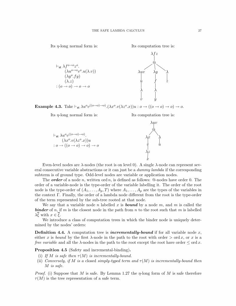
THE SAFE LAMBDA CALCULUS 27
Its η-long normal form is: Its computation tree is:
⊢st λfo→ozo.
(λuo→ovo.u(λ.v))(λyo.fy)(λ.z)
: (o→ o) → o→ o
λfz
@
λuv
u
λ
v
λy
f
λ
y
λ
z
Example 4.3. Take ⊢st λuov((o→o)→o).(λxo.v(λzo.x))u : o→ ((o→ o) → o) → o.
Its η-long normal form is: Its computation tree is:
⊢st λuov((o→o)→o).
(λxo.v(λzo.x))u: o→ ((o→ o) → o) → o
λuv
@
λx
v
λz
x
λ
u
Even-level nodes are λ-nodes (the root is on level 0). A single λ-node can represent sev-eral consecutive variable abstractions or it can just be a dummy lambda if the correspondingsubterm is of ground type. Odd-level nodes are variable or application nodes.
The order of a node n, written ordn, is defined as follows: @-nodes have order 0. Theorder of a variable-node is the type-order of the variable labelling it. The order of the rootnode is the type-order of (A1, . . . , Ap, T ) where A1, . . . , Ap are the types of the variables inthe context Γ. Finally, the order of a lambda node different from the root is the type-orderof the term represented by the sub-tree rooted at that node.
We say that a variable node n labelled x is bound by a node m, and m is called thebinder of n, if m is the closest node in the path from n to the root such that m is labelledλξ with x ∈ ξ.
We introduce a class of computation trees in which the binder node is uniquely deter-mined by the nodes’ orders:
Definition 4.4. A computation tree is incrementally-bound if for all variable node x,either x is bound by the first λ-node in the path to the root with order > ordx, or x is afree variable and all the λ-nodes in the path to the root except the root have order ≤ ordx.
Proposition 4.5 (Safety and incremental-binding).
(i) If M is safe then τ(M) is incrementally-bound.(ii) Conversely, if M is a closed simply-typed term and τ(M) is incrementally-bound then
M is safe.
Proof. (i) Suppose that M is safe. By Lemma 1.27 the η-long form of M is safe thereforeτ(M) is the tree representation of a safe term.
28 W. BLUM AND C.-H. L. ONG
In the safe lambda calculus, the variables in the context with the lowest order must beall abstracted at once when using the abstraction rule. Since the computation tree mergesconsecutive abstractions into a single node, any variable x occurring free in the subtreerooted at a node λξ different from the root must have order greater or equal to ordλξ.Conversely, if a lambda node λξ binds a variable node x then ordλξ = 1 + maxz∈ξ ord z >
ordx.Let x be a bound variable node. Its binder occurs in the path from x to the root,
therefore, according to the previous observation, x must be bound by the first λ-nodeoccurring in this path with order > ordx. Let x be a free variable node then x is notbound by any of the λ-nodes occurring in the path to the root. Once again, by the previousobservation, all these λ-nodes except the root have order smaller than ordx. Hence τ isincrementally-bound.
(ii) Let M be a closed term such that τ(M) is incrementally-bound. W.l.o.g. we canassume that M is in η-long form. We prove that M is safe by induction on its structure.The base case M ≡ λξ.x for some variable x is trivial. Step case: If M ≡ λξ.N1 . . . Np. Leti range over 1..p. We have Ni ≡ ληi.N
′i for some non-abstraction term N ′
i . By the induction
hypothesis, λξ.Ni = λξηi.N′i is a safe closed term, and consequently N ′
i is necessarily safe.Let z be a free variable of N ′
i not bound by ληi in Ni. Since τ(M) is incrementally-boundwe have ord z ≥ ordλη1 = ordNi, thus we can abstract the variables η1 using (abs) whichshows that Ni is safe. Finally we conclude ⊢s M = λξ.N1 . . . Np : T using the rules (app)and (abs).
The assumption that M is closed is necessary. For instance for x, y : o, the computationtrees τ(λxy.x) and τ(λy.x) are both incrementally-bound but λxy.x is safe and λy.x is not.
P-incrementally justified strategy. We now consider the game-semantic model of thesimply-typed lambda calculus. The strategy denotation of a term-in-context Γ ⊢st M : T iswritten [[Γ ⊢st M : T ]]. We define the order of a move m, written ordm, to be the length ofthe path from m to its furthest leaf in the arena minus 1. (There are several ways to definethe order of a move; the definition chosen here is sound in the current setting where eachquestion move in the arena enables at least one answer move.)
Definition 4.6. A strategy σ is said to be P-incrementally justified if for every plays q ∈ σ where q is a P-question, q points to the last unanswered O-question in psq withorder strictly greater than ord q.
Note that although the pointer is determined by the P-view, the choice of the moveitself can be based on the whole history of the play. Thus P-incremental justification doesnot imply innocence.
The definition suggests an algorithm that, given a play of a P-incrementally justifieddenotation, uniquely recovers the pointers from the underlying sequence of moves and fromthe pointers associated to the O-moves therein. Hence:
Lemma 4.7. In P-incrementally justified strategies, pointers emanating from P-moves aresuperfluous.
Example 4.8. Copycat strategies, such as the identity strategy idA on game A or theevaluation map evA,B of type (A⇒ B) ×A→ B, are all P-incrementally justified.6
6In such strategies, a P-move m is justified as follows: Either m points to the preceding move in theP-view or the preceding move is of smaller order and m is justified by the second last O-move in the P-view.
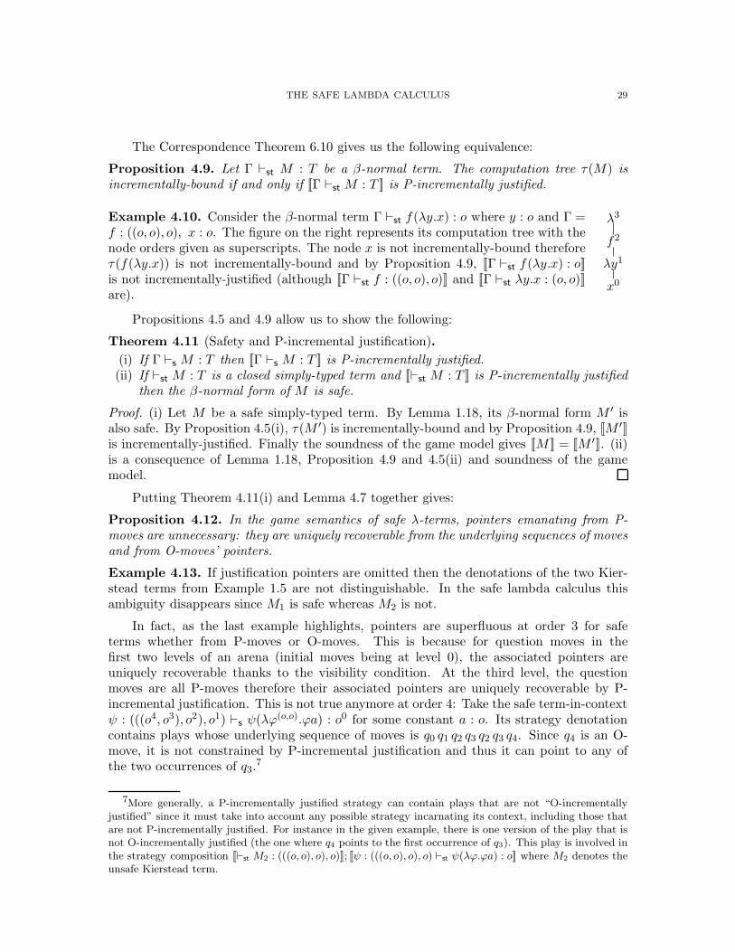
THE SAFE LAMBDA CALCULUS 29
The Correspondence Theorem 6.10 gives us the following equivalence:
Proposition 4.9. Let Γ ⊢st M : T be a β-normal term. The computation tree τ(M) isincrementally-bound if and only if [[Γ ⊢st M : T ]] is P-incrementally justified.
λ3
f2
λy1
x0
Example 4.10. Consider the β-normal term Γ ⊢st f(λy.x) : o where y : o and Γ =f : ((o, o), o), x : o. The figure on the right represents its computation tree with thenode orders given as superscripts. The node x is not incrementally-bound thereforeτ(f(λy.x)) is not incrementally-bound and by Proposition 4.9, [[Γ ⊢st f(λy.x) : o]]is not incrementally-justified (although [[Γ ⊢st f : ((o, o), o)]] and [[Γ ⊢st λy.x : (o, o)]]are).
Propositions 4.5 and 4.9 allow us to show the following:
Theorem 4.11 (Safety and P-incremental justification).
(i) If Γ ⊢s M : T then [[Γ ⊢s M : T ]] is P-incrementally justified.(ii) If ⊢st M : T is a closed simply-typed term and [[⊢st M : T ]] is P-incrementally justified
then the β-normal form of M is safe.
Proof. (i) Let M be a safe simply-typed term. By Lemma 1.18, its β-normal form M ′ isalso safe. By Proposition 4.5(i), τ(M ′) is incrementally-bound and by Proposition 4.9, [[M ′]]is incrementally-justified. Finally the soundness of the game model gives [[M ]] = [[M ′]]. (ii)is a consequence of Lemma 1.18, Proposition 4.9 and 4.5(ii) and soundness of the gamemodel.
Putting Theorem 4.11(i) and Lemma 4.7 together gives:
Proposition 4.12. In the game semantics of safe λ-terms, pointers emanating from P-moves are unnecessary: they are uniquely recoverable from the underlying sequences of movesand from O-moves’ pointers.
Example 4.13. If justification pointers are omitted then the denotations of the two Kier-stead terms from Example 1.5 are not distinguishable. In the safe lambda calculus thisambiguity disappears since M1 is safe whereas M2 is not.
In fact, as the last example highlights, pointers are superfluous at order 3 for safeterms whether from P-moves or O-moves. This is because for question moves in thefirst two levels of an arena (initial moves being at level 0), the associated pointers areuniquely recoverable thanks to the visibility condition. At the third level, the questionmoves are all P-moves therefore their associated pointers are uniquely recoverable by P-incremental justification. This is not true anymore at order 4: Take the safe term-in-contextψ : (((o4, o3), o2), o1) ⊢s ψ(λϕ(o,o).ϕa) : o0 for some constant a : o. Its strategy denotationcontains plays whose underlying sequence of moves is q0 q1 q2 q3 q2 q3 q4. Since q4 is an O-move, it is not constrained by P-incremental justification and thus it can point to any ofthe two occurrences of q3.
7
7More generally, a P-incrementally justified strategy can contain plays that are not “O-incrementallyjustified” since it must take into account any possible strategy incarnating its context, including those thatare not P-incrementally justified. For instance in the given example, there is one version of the play that isnot O-incrementally justified (the one where q4 points to the first occurrence of q3). This play is involved inthe strategy composition [[⊢st M2 : (((o, o), o), o)]]; [[ψ : (((o, o), o), o) ⊢st ψ(λϕ.ϕa) : o]] where M2 denotes theunsafe Kierstead term.
30 W. BLUM AND C.-H. L. ONG
Towards a fully abstract game model. The standard game models which have beenshown to be fully abstract for PCF [2, 18] are of course also fully abstract for the restrictedlanguage safe PCF. One may ask, however, whether there exists a fully abstract model withrespect to safe context only. Such model may be obtained by considering P-incrementallyjustified strategies—which have been shown to compose [7]. Its is reasonable to think thatO-moves also needs to be constrained by the symmetrical O-incremental justification, whichcorresponds to the requirement that contexts are safe. This line of work is still in progress.
Safe PCF and safe Idealised Algol. PCF is the simply-typed lambda calculus aug-mented with basic arithmetic operators, if-then-else branching and a family of recursioncombinator YA : ((A,A), A) for every type A. We define safe PCF to be PCF where theapplication and abstraction rules are constrained in the same way as the safe lambda cal-culus. This language inherits the good properties of the safe lambda calculus: No variablecapture occurs when performing substitution and safety is preserved by the reduction rulesof the small-step semantics of PCF.
Correspondence. The computation tree of a PCF term is defined as the least upper-bound ofthe chain of computation trees of its syntactic approximants [3]. It is obtained by infinitelyexpanding the Y combinator, for instance τ(Y (λfx.fx)) is the tree representation of theη-long form of the infinite term (λfx.fx)((λfx.fx)((λfx.fx)(. . .
It is straightforward to define the traversal rules modeling the arithmetic constants ofPCF. Just as in the safe lambda calculus we had to remove @-nodes in order to reveal thegame-semantic correspondence, in safe PCF it is necessary to filter out the constant nodesfrom the traversals. The Correspondence Theorem for PCF says that the revealed gamesemantics is isomorphic to the set of traversals disposed of these superfluous nodes. Thiscan easily be shown for term approximants. It is then lifted to full PCF using the continuityof the function T rv( )↾⊛ from the set of computation trees (ordered by the approximationordering) to the set of sets of justified sequences of nodes (ordered by subset inclusion).Finally computation trees of safe PCF terms are incrementally-bound thus we have
Theorem 4.14. Safe PCF terms have P-incrementally justified denotations.
Similarly, we can define safe IA to be safe PCF augmented with the imperative featuresof Idealized Algol (IA for short) [32]. Adapting the game-semantic correspondence andsafety characterization to IA seems feasible although the presence of the base type var,whose game arena comN×exp has infinitely many initial moves, causes a mismatch betweenthe simple tree representation of the term and its game arena. It may be possible toovercome this problem by replacing the notion of computation tree by a “computationdirected acyclic graph”.
The possibility of representing plays without some or all of their pointers under thesafety assumption suggests potential applications in algorithmic game semantics. Ghicaand McCusker [15] were the first to observe that pointers are unnecessary for representingplays in the game semantics of the second-order finitary fragment of Idealized Algol (IA2
for short). Consequently observational equivalence for this fragment can be reduced to theproblem of equivalence of regular expressions. At order 3, although pointers are necessary,deciding observational equivalence of IA3 is EXPTIME-complete [29, 28]. Restricting theproblem to the safe fragment of IA3 may lead to a lower complexity.
THE SAFE LAMBDA CALCULUS 31
5. Further work and open problems
The safe lambda calculus is still not well understood. Many basic questions remain.What is a (categorical) model of the safe lambda calculus? Does the calculus have inter-esting models? What kind of reasoning principles does the safe lambda calculus support,via the Curry-Howard Isomorphism? Does the safe lambda calculus characterize a com-plexity class, in the same way that the simply-typed lambda calculus characterizes thepolytime-computable numeric functions [21]? Is the addition of unsafe contexts to safe onesconservative with respect to observational (or contextual) equivalence?
With a view to algorithmic game semantics and its applications, it would be interest-ing to identify sublanguages of Idealised Algol whose game semantics enjoy the propertythat pointers in a play are uniquely recoverable from the underlying sequence of moves.We name this class PUR. IA2 is the paradigmatic example of a PUR-language. Anotherexample is Serially Re-entrant Idealized Algol [1], a version of IA where multiple uses ofarguments are allowed only if they do not “overlap in time”. We believe that a PUR lan-guage can be obtained by imposing the safety condition on IA3. Murawski [27] has shownthat observational equivalence for IA4 is undecidable; is observational equivalence for safeIA4 decidable?
Acknowledgment. We thank Ugo dal Lago for the insightful discussions we had during hisvisit at the Oxford University Computing Laboratory in March 2008, and the anonymousreferees for helpful comments.
References
[1] S. Abramsky. Semantics via game theory. In Marktoberdorf International Summer School, 2001. Lectureslides.
[2] S. Abramsky, P. Malacaria, and R. Jagadeesan. Full abstraction for PCF. In Theoretical Aspects of
Computer Software, pages 1–15, 1994.[3] S. Abramsky and G. McCusker. Game semantics. In H. Schwichtenberg and U. Berger, editors, Logic
and Computation: Proceedings of the 1997 Marktoberdorf Summer School, pages 1–56. Springer-Verlag,1998. Lecture notes.
[4] K. Aehlig, J. G. de Miranda, and C.-H. L. Ong. Safety is not a restriction at level 2 for string languages.Technical report, University of Oxford, 2004.
[5] A. V. Aho. Indexed grammars – an extension of context-free grammars. J. ACM, 15(4):647–671, 1968.[6] A. Asperti. P = NP, up to sharing.[7] W. Blum. The Safe Lambda Calculus. PhD thesis, University of Oxford, forthcoming.[8] W. Blum and C.-H. L. Ong. The safe lambda calculus. In S. R. D. Rocca, editor, TLCA, volume 4583
of Lecture Notes in Computer Science, pages 39–53. Springer, 2007.[9] D. Caucal. On infinite terms having a decidable monadic theory. Lecture Notes in Computer Science,
2420:165–176, 2002.[10] W. Damm. The IO- and OI-hierarchy. TCS, 20:95–207, 1982.[11] W. Damm and A. Goerdt. An automata-theoretical characterization of the OI-hierarchy. Information
and Control, 71(1-2):1–32, 1986.[12] J. G. de Miranda. Structures generated by higher-order grammars and the safety constraint. D.Phil
thesis, University of Oxford, 2006.[13] A. Dimovski, D. R. Ghica, and R. Lazic. Data-abstraction refinement: A game semantic approach. In
C. Hankin and I. Siveroni, editors, SAS, volume 3672 of Lecture Notes in Computer Science, pages102–117. Springer, 2005.
[14] S. Fortune, D. Leivant, and M. O’Donnell. The expressiveness of simple and second-order type struc-tures. J. ACM, 30(1):151–185, 1983.
32 W. BLUM AND C.-H. L. ONG
[15] D. R. Ghica and G. McCusker. Reasoning about idealized algol using regular languages. In Proceedings
of 27th International Colloquium on Automata, Languages and Programming ICALP 2000, volume 1853of LNCS, pages 103–116. Springer-Verlag, 2000.
[16] W. Greenland. Game Semantics for Region Analysis. PhD thesis, University of Oxford, 2004.[17] M. Hague, A. S. Murawski, C.-H. L. Ong, and O. Serre. Collapsible pushdown automata and recursive
schemes. LICS, pages 452–461, 2008.[18] J. M. E. Hyland and C.-H. L. Ong. On full abstraction for PCF: I, II, and III. Information and Com-
putation, 163(2):285–408, December 2000.[19] T. Knapik, D. Niwinski, and P. Urzyczyn. Higher-order pushdown trees are easy. In FOSSACS’02, pages
205–222. Springer, 2002. LNCS Vol. 2303.[20] D. Leivant. Functions over free algebras definable in the simply typed lambda calculus. Theor. Comput.
Sci., 121(1&2):309–322, 1993.[21] D. Leivant and J.-Y. Marion. Lambda calculus characterizations of poly-time. In M. Bezem and J. F.
Groote, editors, TLCA, volume 664 of Lecture Notes in Computer Science, pages 274–288. Springer,1993.
[22] R. Loader. Notes on simply typed lambda calculus, February 1998.[23] H. G. Mairson. A Simple Proof of a Theorem of Statman. TCS, 103(2):387–394, 1992.[24] A. N. Maslov. The hierarchy of indexed languages of an arbitrary level. Soviet Math. Dokl., 15:1170–
1174, 1974.[25] A. N. Maslov. Multilevel stack automata. Problems of Information Transmission, 12:38–43, 1976.[26] A. R. Meyer. The inherent computational complexity of theories of ordered sets. In Proc. Int’l. Cong.
of Mathematicians, volume 2, pages 477–482, August 1974.[27] A. S. Murawski. On program equivalence in languages with ground-type references. In Logic in Computer
Science, 2003. Proceedings. 18th Annual IEEE Symposium on, pages 108–117, 22-25 June 2003.[28] A. S. Murawski and I. Walukiewicz. Third-order idealized algol with iteration is decidable. In V. Sassone,
editor, FoSSaCS, volume 3441 of Lecture Notes in Computer Science, pages 202–218. Springer, 2005.[29] C.-H. L. Ong. An approach to deciding observational equivalence of algol-like languages. Ann. Pure
Appl. Logic, 130(1-3):125–171, 2004.[30] C.-H. L. Ong. On model-checking trees generated by higher-order recursion schemes. In Proceedings of
IEEE Symposium on Logic in Computer Science., pages 81–90. Computer Society Press, 2006. Extendedabstract.
[31] C.-H. L. Ong. On model-checking trees generated by higher-order recursion schemes (technical report).Preprint, 42 pp, 2006.
[32] J. C. Reynolds. The essence of algol. In J. W. de Bakker and J. C. van Vliet, editors, Algorithmic
Languages, pages 345–372. IFIP, North-Holland, Amsterdam, 1981.[33] A. Schubert. The complexity of beta-reduction in low orders. Proceedings TLCA 2001, pages 400–414,
2001.[34] H. Schwichtenberg. Definierbare funktionen im lambda-kalkul mit typen. Archiv Logik Grundlagen-
forsch, 17:113–114, 1976.[35] R. Statman. Intuitionistic propositional logic is polynomial-space complete. Theoretical Computer Sci-
ence, 9(1):67–72, July 1979.[36] R. Statman. The typed lambda-calculus is not elementary recursive. Theoretical Computer Science,
9(1):73–81, July 1979.[37] M. Zaionc. Word operation definable in the typed lambda-calculus. Theor. Comput. Sci., 52:1–14, 1987.[38] M. Zaionc. On the lambda-definable tree operations. In C. Bergman, R. D. Maddux, and D. Pigozzi,
editors, Algebraic Logic and Universal Algebra in Computer Science, volume 425 of Lecture Notes in
Computer Science, pages 279–292. Springer, 1988.[39] M. Zaionc. Lambda-definability on free algebras. Ann. Pure Appl. Logic, 51(3):279–300, 1991.[40] M. Zaionc. Lambda representation of operations between different term algebras. Lecture Notes in
Computer Science, pages 91–105, 1995.
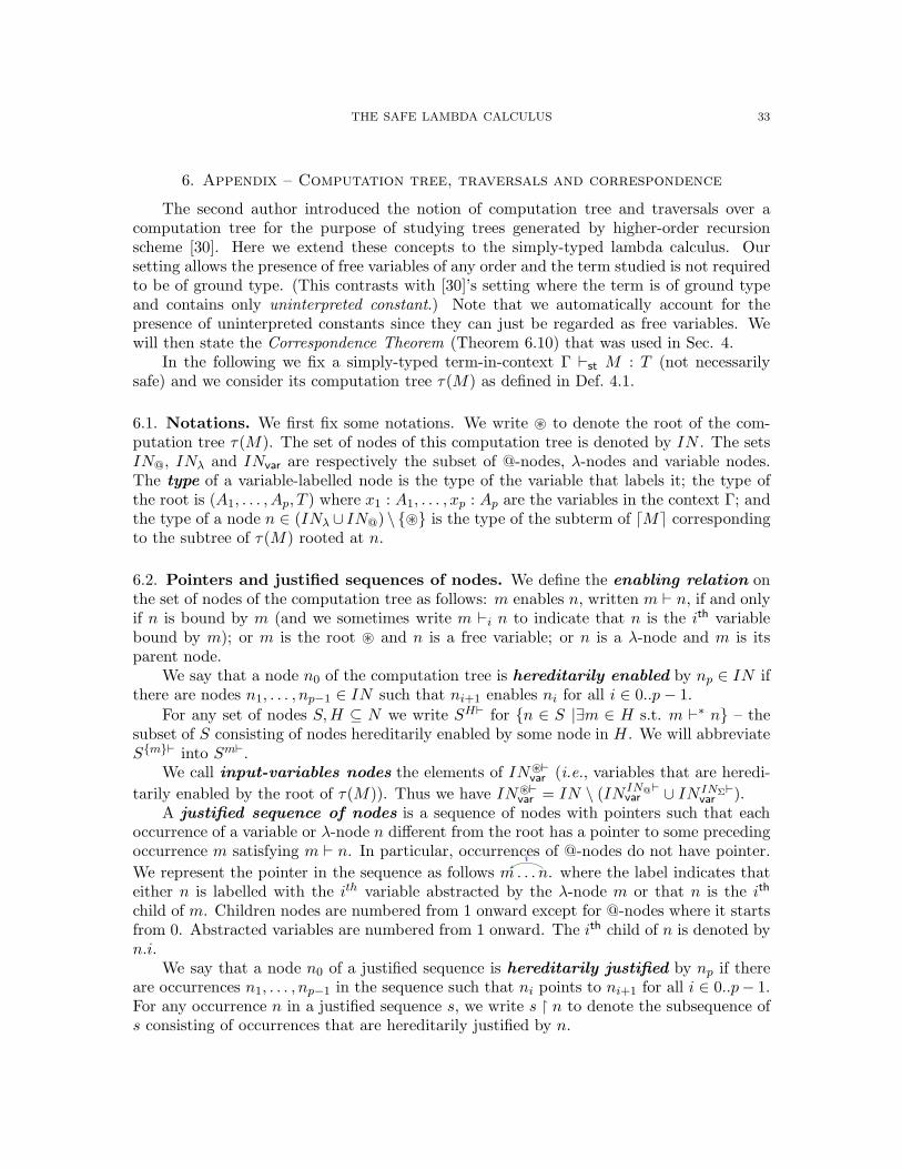
THE SAFE LAMBDA CALCULUS 33
6. Appendix – Computation tree, traversals and correspondence
The second author introduced the notion of computation tree and traversals over acomputation tree for the purpose of studying trees generated by higher-order recursionscheme [30]. Here we extend these concepts to the simply-typed lambda calculus. Oursetting allows the presence of free variables of any order and the term studied is not requiredto be of ground type. (This contrasts with [30]’s setting where the term is of ground typeand contains only uninterpreted constant.) Note that we automatically account for thepresence of uninterpreted constants since they can just be regarded as free variables. Wewill then state the Correspondence Theorem (Theorem 6.10) that was used in Sec. 4.
In the following we fix a simply-typed term-in-context Γ ⊢st M : T (not necessarilysafe) and we consider its computation tree τ(M) as defined in Def. 4.1.
6.1. Notations. We first fix some notations. We write ⊛ to denote the root of the com-putation tree τ(M). The set of nodes of this computation tree is denoted by IN . The setsIN@, INλ and INvar are respectively the subset of @-nodes, λ-nodes and variable nodes.The type of a variable-labelled node is the type of the variable that labels it; the type ofthe root is (A1, . . . , Ap, T ) where x1 : A1, . . . , xp : Ap are the variables in the context Γ; andthe type of a node n ∈ (INλ ∪ IN@) \ {⊛} is the type of the subterm of ⌈M⌉ correspondingto the subtree of τ(M) rooted at n.
6.2. Pointers and justified sequences of nodes. We define the enabling relation onthe set of nodes of the computation tree as follows: m enables n, written m ⊢ n, if and onlyif n is bound by m (and we sometimes write m ⊢i n to indicate that n is the ith variablebound by m); or m is the root ⊛ and n is a free variable; or n is a λ-node and m is itsparent node.
We say that a node n0 of the computation tree is hereditarily enabled by np ∈ IN ifthere are nodes n1, . . . , np−1 ∈ IN such that ni+1 enables ni for all i ∈ 0..p − 1.
For any set of nodes S,H ⊆ N we write SH⊢ for {n ∈ S |∃m ∈ H s.t. m ⊢∗ n} – thesubset of S consisting of nodes hereditarily enabled by some node in H. We will abbreviateS{m}⊢ into Sm⊢.
We call input-variables nodes the elements of IN⊛⊢var (i.e., variables that are heredi-
tarily enabled by the root of τ(M)). Thus we have IN⊛⊢var = IN \ (IN IN@⊢
var ∪ IN INΣ⊢var ).
A justified sequence of nodes is a sequence of nodes with pointers such that eachoccurrence of a variable or λ-node n different from the root has a pointer to some precedingoccurrence m satisfying m ⊢ n. In particular, occurrences of @-nodes do not have pointer.
We represent the pointer in the sequence as follows m. . . ni
. where the label indicates thateither n is labelled with the ith variable abstracted by the λ-node m or that n is the ith
child of m. Children nodes are numbered from 1 onward except for @-nodes where it startsfrom 0. Abstracted variables are numbered from 1 onward. The ith child of n is denoted byn.i.
We say that a node n0 of a justified sequence is hereditarily justified by np if thereare occurrences n1, . . . , np−1 in the sequence such that ni points to ni+1 for all i ∈ 0..p− 1.For any occurrence n in a justified sequence s, we write s ↾ n to denote the subsequence ofs consisting of occurrences that are hereditarily justified by n.
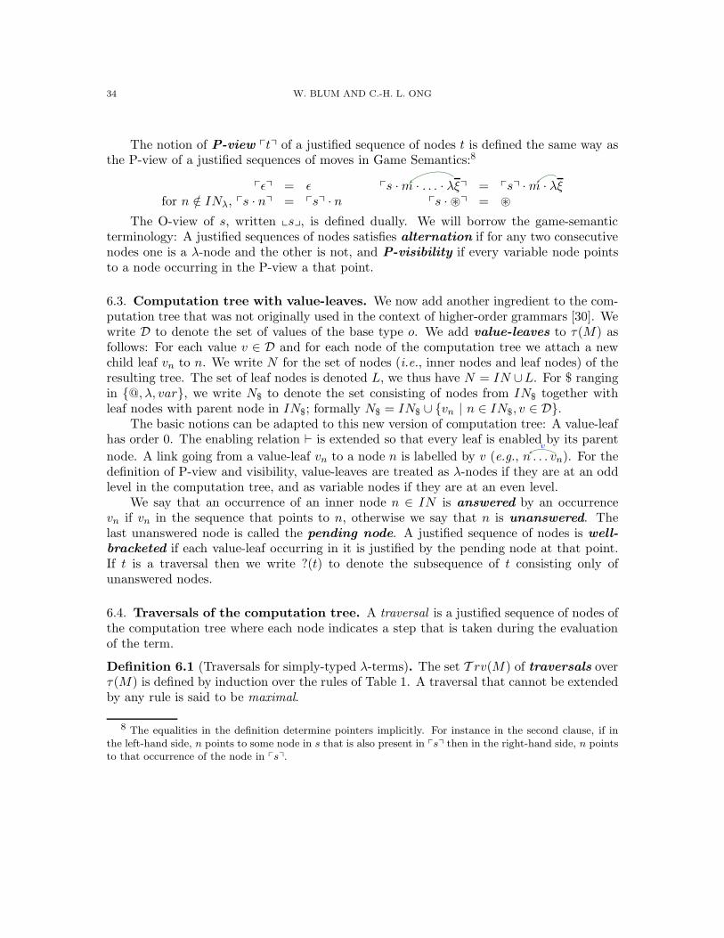
34 W. BLUM AND C.-H. L. ONG
The notion of P-view ptq of a justified sequence of nodes t is defined the same way asthe P-view of a justified sequences of moves in Game Semantics:8
pǫq = ǫ ps ·m · . . . · λξq = psq ·m · λξfor n /∈ INλ, ps · nq = psq · n ps · ⊛q = ⊛
The O-view of s, written xsy, is defined dually. We will borrow the game-semanticterminology: A justified sequences of nodes satisfies alternation if for any two consecutivenodes one is a λ-node and the other is not, and P-visibility if every variable node pointsto a node occurring in the P-view a that point.
6.3. Computation tree with value-leaves. We now add another ingredient to the com-putation tree that was not originally used in the context of higher-order grammars [30]. Wewrite D to denote the set of values of the base type o. We add value-leaves to τ(M) asfollows: For each value v ∈ D and for each node of the computation tree we attach a newchild leaf vn to n. We write N for the set of nodes (i.e., inner nodes and leaf nodes) of theresulting tree. The set of leaf nodes is denoted L, we thus have N = IN ∪L. For $ rangingin {@, λ, var}, we write N$ to denote the set consisting of nodes from IN$ together withleaf nodes with parent node in IN$; formally N$ = IN$ ∪ {vn | n ∈ IN$, v ∈ D}.
The basic notions can be adapted to this new version of computation tree: A value-leafhas order 0. The enabling relation ⊢ is extended so that every leaf is enabled by its parent
node. A link going from a value-leaf vn to a node n is labelled by v (e.g., n . . . vn
v
). For thedefinition of P-view and visibility, value-leaves are treated as λ-nodes if they are at an oddlevel in the computation tree, and as variable nodes if they are at an even level.
We say that an occurrence of an inner node n ∈ IN is answered by an occurrencevn if vn in the sequence that points to n, otherwise we say that n is unanswered. Thelast unanswered node is called the pending node. A justified sequence of nodes is well-
bracketed if each value-leaf occurring in it is justified by the pending node at that point.If t is a traversal then we write ?(t) to denote the subsequence of t consisting only ofunanswered nodes.
6.4. Traversals of the computation tree. A traversal is a justified sequence of nodes ofthe computation tree where each node indicates a step that is taken during the evaluationof the term.
Definition 6.1 (Traversals for simply-typed λ-terms). The set T rv(M) of traversals overτ(M) is defined by induction over the rules of Table 1. A traversal that cannot be extendedby any rule is said to be maximal.
8 The equalities in the definition determine pointers implicitly. For instance in the second clause, if inthe left-hand side, n points to some node in s that is also present in psq then in the right-hand side, n pointsto that occurrence of the node in psq.
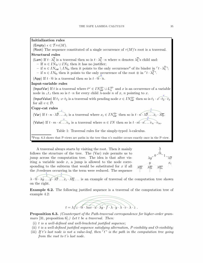
THE SAFE LAMBDA CALCULUS 35
Initialization rules
(Empty) ǫ ∈ T rv(M).(Root) The sequence constituted of a single occurrence of τ(M)’s root is a traversal.
Structural rules
(Lam) If t · λξ is a traversal then so is t · λξ · n where n denotes λξ’s child and:– If n ∈ IN@ ∪ INΣ then it has no justifier;– if n ∈ INvar \ INfv then it points to the only occurrencea of its binder in pt · λξq;– if n ∈ INfv then it points to the only occurrence of the root ⊛ in pt · λξq.
(App) If t · @ is a traversal then so is t · @ · n0
.
Input-variable rules
(InputVar) If t is a traversal where tω ∈ IN⊛⊢var ∪L
⊛⊢λ and x is an occurrence of a variable
node in xty then so is t · n for every child λ-node n of x, n pointing to x.
(InputValue) If t1 ·x·t2 is a traversal with pending node x ∈ IN⊛⊢var then so is t1 · x · t2 · vx
v
for all v ∈ D.
Copy-cat rules
(Var) If t · n · λx . . . xi
i
is a traversal where xi ∈ IN@⊢var then so is t · n · λx . . . xi
i
· ληi
i
.
(Value) If t ·m · n . . . vv
n is a traversal where n ∈ IN then so is t ·m · n . . . vv
n · v
v
m.
Table 1: Traversal rules for the simply-typed λ-calculus.
aProp. 6.3 shows that P-views are paths in the tree thus n’s enabler occurs exactly once in the P-view.
λ
@
λy0
y
λη1...ληi...
ληn...
λx1
xi
A traversal always starts by visiting the root. Then it mainlyfollows the structure of the tree. The (Var) rule permits us tojump across the computation tree. The idea is that after vis-iting a variable node x, a jump is allowed to the node corre-sponding to the subterm that would be substituted for x if allthe β-redexes occurring in the term were reduced. The sequence
λ · @ · λy . . . y1
· λx
1
. . . xi
i
· ληi
i
. . . is an example of traversal of the computation tree shownon the right.
Example 6.2. The following justified sequence is a traversal of the computation tree ofexample 4.2:
t = λfz · @ · λuv · u · λy · f · λ · y · λ · v · λ · z .
Proposition 6.3. (Counterpart of the Path-traversal correspondence for higher-order gram-mars [31, proposition 6].) Let t be a traversal. Then:
(i) t is a well-defined and well-bracketed justified sequence;(ii) t is a well-defined justified sequence satisfying alternation, P-visibility and O-visibility;(iii) If t’s last node is not a value-leaf, then ptq is the path in the computation tree going
from the root to t’s last node.
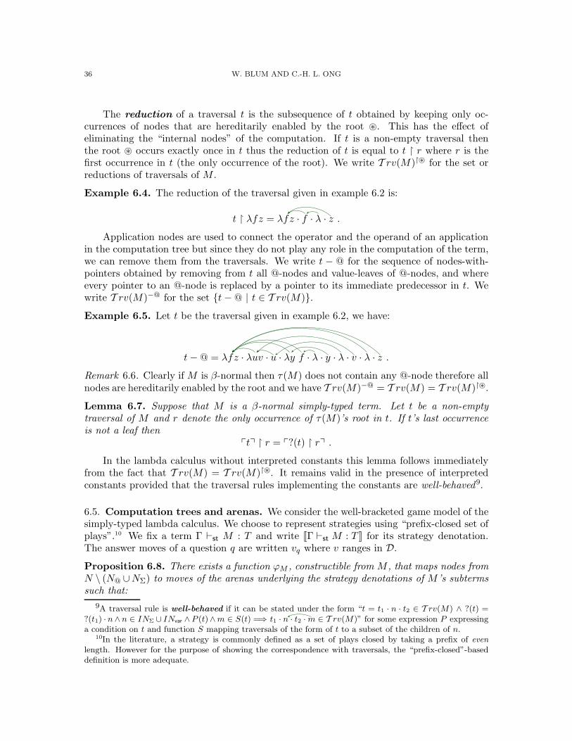
36 W. BLUM AND C.-H. L. ONG
The reduction of a traversal t is the subsequence of t obtained by keeping only oc-currences of nodes that are hereditarily enabled by the root ⊛. This has the effect ofeliminating the “internal nodes” of the computation. If t is a non-empty traversal thenthe root ⊛ occurs exactly once in t thus the reduction of t is equal to t ↾ r where r is thefirst occurrence in t (the only occurrence of the root). We write T rv(M)↾⊛ for the set orreductions of traversals of M .
Example 6.4. The reduction of the traversal given in example 6.2 is:
t ↾ λfz = λfz · f · λ · z .
Application nodes are used to connect the operator and the operand of an applicationin the computation tree but since they do not play any role in the computation of the term,we can remove them from the traversals. We write t − @ for the sequence of nodes-with-pointers obtained by removing from t all @-nodes and value-leaves of @-nodes, and whereevery pointer to an @-node is replaced by a pointer to its immediate predecessor in t. Wewrite T rv(M)−@ for the set {t− @ | t ∈ T rv(M)}.
Example 6.5. Let t be the traversal given in example 6.2, we have:
t− @ = λfz · λuv · u · λy f · λ · y · λ · v · λ · z .
Remark 6.6. Clearly if M is β-normal then τ(M) does not contain any @-node therefore allnodes are hereditarily enabled by the root and we have T rv(M)−@ = T rv(M) = T rv(M)↾⊛.
Lemma 6.7. Suppose that M is a β-normal simply-typed term. Let t be a non-emptytraversal of M and r denote the only occurrence of τ(M)’s root in t. If t’s last occurrenceis not a leaf then
ptq ↾ r = p?(t) ↾ rq .
In the lambda calculus without interpreted constants this lemma follows immediatelyfrom the fact that T rv(M) = T rv(M)↾⊛. It remains valid in the presence of interpretedconstants provided that the traversal rules implementing the constants are well-behaved9.
6.5. Computation trees and arenas. We consider the well-bracketed game model of thesimply-typed lambda calculus. We choose to represent strategies using “prefix-closed set ofplays”.10 We fix a term Γ ⊢st M : T and write [[Γ ⊢st M : T ]] for its strategy denotation.The answer moves of a question q are written vq where v ranges in D.
Proposition 6.8. There exists a function ϕM , constructible from M , that maps nodes fromN \ (N@ ∪NΣ) to moves of the arenas underlying the strategy denotations of M ’s subtermssuch that:
9A traversal rule is well-behaved if it can be stated under the form “t = t1 · n · t2 ∈ T rv(M) ∧ ?(t) =?(t1) · n∧n ∈ INΣ ∪ INvar ∧ P (t)∧m ∈ S(t) =⇒ t1 · n · t2 ·m ∈ T rv(M)” for some expression P expressinga condition on t and function S mapping traversals of the form of t to a subset of the children of n.
10In the literature, a strategy is commonly defined as a set of plays closed by taking a prefix of even
length. However for the purpose of showing the correspondence with traversals, the “prefix-closed”-baseddefinition is more adequate.
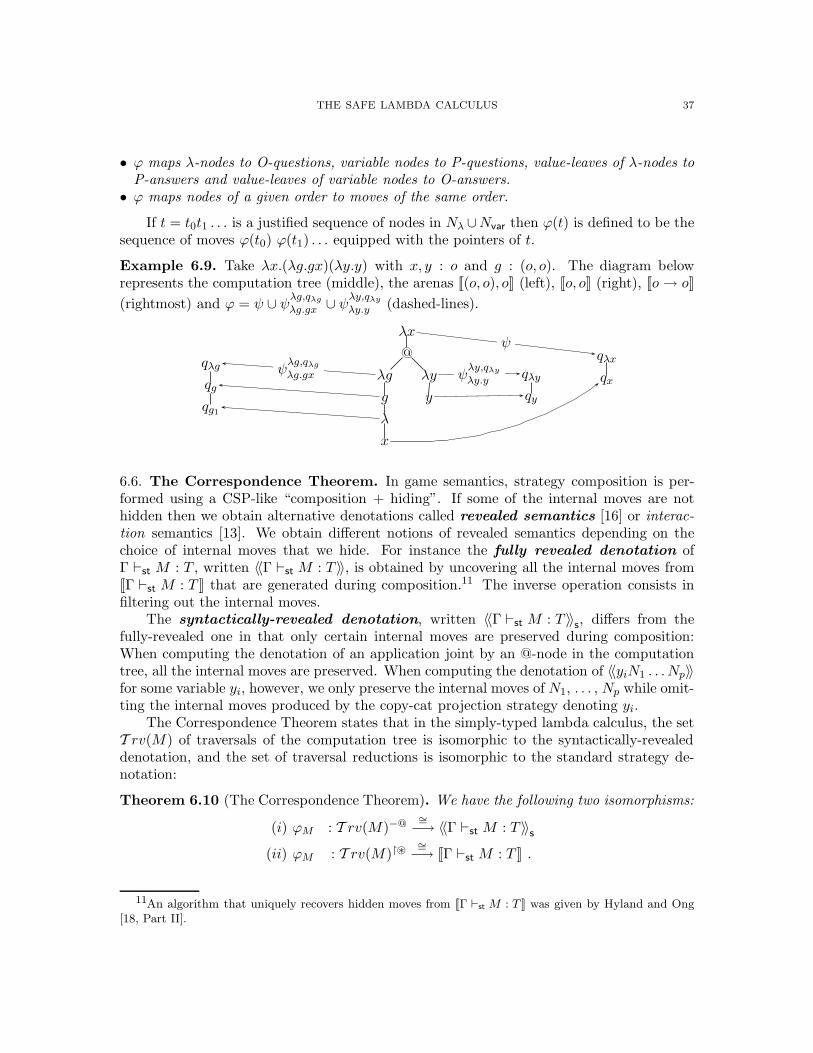
THE SAFE LAMBDA CALCULUS 37
• ϕ maps λ-nodes to O-questions, variable nodes to P-questions, value-leaves of λ-nodes toP-answers and value-leaves of variable nodes to O-answers.
• ϕ maps nodes of a given order to moves of the same order.
If t = t0t1 . . . is a justified sequence of nodes in Nλ ∪Nvar then ϕ(t) is defined to be thesequence of moves ϕ(t0) ϕ(t1) . . . equipped with the pointers of t.
Example 6.9. Take λx.(λg.gx)(λy.y) with x, y : o and g : (o, o). The diagram belowrepresents the computation tree (middle), the arenas [[(o, o), o]] (left), [[o, o]] (right), [[o→ o]]
(rightmost) and ϕ = ψ ∪ ψλg,qλg
λg.gx ∪ ψλy,qλy
λy.y (dashed-lines).
λx
@
λg
g
λ
x
λy
y
qλx
qxqλg
qg
qg1
qλy
qy
ψ
ψλg,qλg
λg.gx ψλy,qλy
λy.y
6.6. The Correspondence Theorem. In game semantics, strategy composition is per-formed using a CSP-like “composition + hiding”. If some of the internal moves are nothidden then we obtain alternative denotations called revealed semantics [16] or interac-tion semantics [13]. We obtain different notions of revealed semantics depending on thechoice of internal moves that we hide. For instance the fully revealed denotation ofΓ ⊢st M : T , written 〈〈Γ ⊢st M : T 〉〉, is obtained by uncovering all the internal moves from[[Γ ⊢st M : T ]] that are generated during composition.11 The inverse operation consists infiltering out the internal moves.
The syntactically-revealed denotation, written 〈〈Γ ⊢st M : T 〉〉s, differs from the
fully-revealed one in that only certain internal moves are preserved during composition:When computing the denotation of an application joint by an @-node in the computationtree, all the internal moves are preserved. When computing the denotation of 〈〈yiN1 . . . Np〉〉for some variable yi, however, we only preserve the internal moves of N1, . . . , Np while omit-ting the internal moves produced by the copy-cat projection strategy denoting yi.
The Correspondence Theorem states that in the simply-typed lambda calculus, the setT rv(M) of traversals of the computation tree is isomorphic to the syntactically-revealeddenotation, and the set of traversal reductions is isomorphic to the standard strategy de-notation:
Theorem 6.10 (The Correspondence Theorem). We have the following two isomorphisms:
(i) ϕM : T rv(M)−@∼=−→ 〈〈Γ ⊢st M : T 〉〉
s
(ii) ϕM : T rv(M)↾⊛∼=
−→ [[Γ ⊢st M : T ]] .
11An algorithm that uniquely recovers hidden moves from [[Γ ⊢st M : T ]] was given by Hyland and Ong[18, Part II].
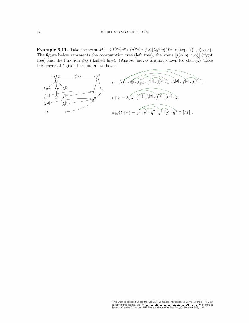
38 W. BLUM AND C.-H. L. ONG
Example 6.11. Take the term M ≡ λf (o,o)zo.(λg(o,o)x.fx)(λyo.y)(fz) of type ((o, o), o, o).The figure below represents the computation tree (left tree), the arena [[((o, o), o, o)]] (righttree) and the function ψM (dashed line). (Answer moves are not shown for clarity.) Takethe traversal t given hereunder, we have:
λfz@
λgx
f [1]
λ[2]
x
λy
y
λ[3]
f [4]
λ[5]
z
q0
q1
q2
q3
ψM
t = λfz · @ · λgx · f [1] · λ[2] · x · λ[3] · f [4] · λ[5] · z
t ↾ r = λfz · f [1] · λ[2] · f [4] · λ[5] · z
ϕM (t ↾ r) = q0 · q1 · q2 · q1 · q2 · q3 ∈ [[M ]] .
This work is licensed under the Creative Commons Attribution-NoDerivs License. To viewa copy of this license, visit http:// reative ommons.org/li enses/by-nd/2.0/ or send aletter to Creative Commons, 559 Nathan Abbott Way, Stanford, California 94305, USA.