Embed Size (px)
Citation preview
The ROMES method forreduced-order-model uncertainty quantification:
application to data assimilation
M. Drohmann and K. Carlberg
Sandia National Laboratories
Workshop on Model Order Reduction and DataParis, France
January 6, 2014
ROMES M. Drohmann and K. Carlberg 1 / 24
Data assimilation by Bayesian inference
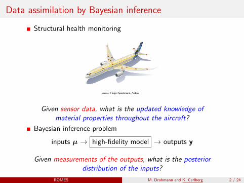
Structural health monitoring
source: Theoretical & Computational Biophysics Group, UIUCsource: Holger Speckmann, Airbus
Given sensor data, what is the updated knowledge ofmaterial properties throughout the aircraft?
Bayesian inference problem
inputs µ → high-fidelity model → outputs y
Given measurements of the outputs, what is the posteriordistribution of the inputs?
ROMES M. Drohmann and K. Carlberg 2 / 24
Bayesian inference
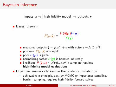
inputs µ → high-fidelity model → outputs y
Bayes’ theorem
P(µ|y) =P (y|µ)P(µ)
P(y)
measured outputs y = y(µ?) + ε with noise ε ∼ N (0, σ2I)posterior P(µ|y) is soughtprior P (µ) is givennormalizing factor P (y) is handled indirectlylikelihood P (y|µ) ∼ N (y(µ), σ2I) sampling requireshigh-fidelity model evaluations
Objective: numerically sample the posterior distribution
+ achievable in principle, e.g., by MCMC or importance sampling.- barrier: sampling requires high-fidelity forward solves
ROMES M. Drohmann and K. Carlberg 3 / 24
Reduced-order modeling and Bayesian inference
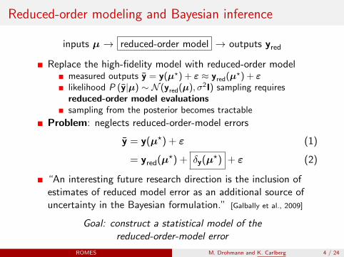
inputs µ → reduced-order model → outputs yred
Replace the high-fidelity model with reduced-order modelmeasured outputs y = y(µ?) + ε ≈ yred(µ?) + εlikelihood P (y|µ) ∼ N (yred(µ), σ2I) sampling requiresreduced-order model evaluationssampling from the posterior becomes tractable
Problem: neglects reduced-order-model errors
y = y(µ?) + ε (1)
= yred(µ?) + δy(µ?) + ε (2)
“An interesting future research direction is the inclusion ofestimates of reduced model error as an additional source ofuncertainty in the Bayesian formulation.” [Galbally et al., 2009]
Goal: construct a statistical model of thereduced-order-model error
ROMES M. Drohmann and K. Carlberg 4 / 24
Strategies for ROM error quantification
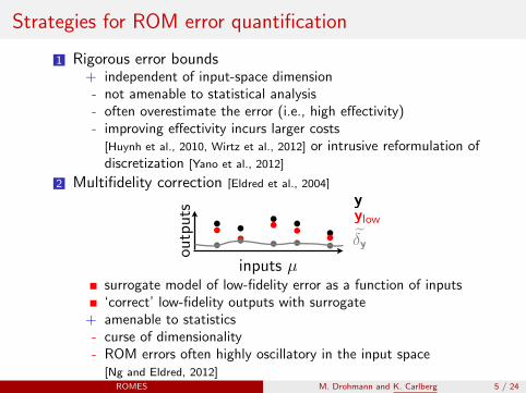
1 Rigorous error bounds+ independent of input-space dimension- not amenable to statistical analysis- often overestimate the error (i.e., high effectivity)- improving effectivity incurs larger costs
[Huynh et al., 2010, Wirtz et al., 2012] or intrusive reformulation ofdiscretization [Yano et al., 2012]
2 Multifidelity correction [Eldred et al., 2004]
y
eyylow
inputs µ
outp
uts
surrogate model of low-fidelity error as a function of inputs‘correct’ low-fidelity outputs with surrogate
+ amenable to statistics- curse of dimensionality- ROM errors often highly oscillatory in the input space
[Ng and Eldred, 2012]ROMES M. Drohmann and K. Carlberg 5 / 24
Our key observation
10−5 10−4
10−5
10−4
Residual r/error bound
error(energy
norm
)|||u
h−
ure
d|||
10−5
10−4
10−5
10−4
10−5
10−4
Residual r error b
ound
error(energy
norm
)|||u
h−
ure
d|||
(r; |||δu|||)(∆µ
u ; |||δu|||)
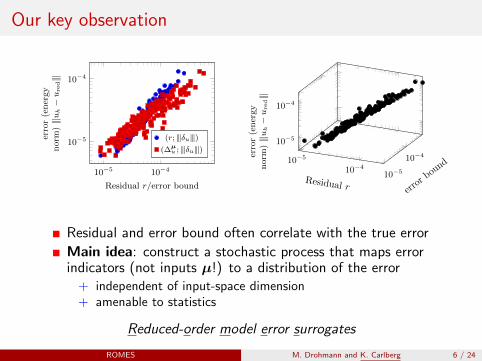
Residual and error bound often correlate with the true error
Main idea: construct a stochastic process that maps errorindicators (not inputs µ!) to a distribution of the error
+ independent of input-space dimension+ amenable to statistics
Reduced-order model error surrogates
ROMES M. Drohmann and K. Carlberg 6 / 24
ROMES
y
eyylow
inputs µ
outp
uts
105 104
105
104
residual R
erro
r(e
ner
gy
norm
)|||u
h
ure
d|||
(i) Kernel method
105 104
106
104
residual R
erro
r(e
ner
gy
norm
)|||u
h
ure
d|||
(ii) RVM
training point mean 95% confidence “uncertainty of mean”
error
error indicator
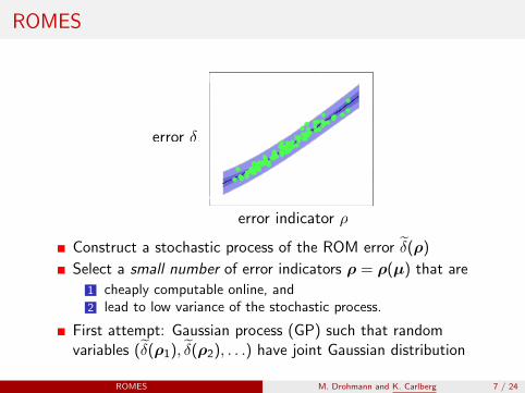
Construct a stochastic process of the ROM error δ(ρ)
Select a small number of error indicators ρ = ρ(µ) that are
1 cheaply computable online, and2 lead to low variance of the stochastic process.
First attempt: Gaussian process (GP) such that randomvariables (δ(ρ1), δ(ρ2), . . .) have joint Gaussian distribution
ROMES M. Drohmann and K. Carlberg 7 / 24
Gaussian process [Rasmussen and Williams, 2006]
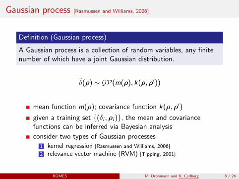
Definition (Gaussian process)
A Gaussian process is a collection of random variables, any finitenumber of which have a joint Gaussian distribution.
δ(ρ) ∼ GP(m(ρ), k(ρ,ρ′))
mean function m(ρ); covariance function k(ρ,ρ′)
given a training set (δi ,ρi ), the mean and covariancefunctions can be inferred via Bayesian analysis
consider two types of Gaussian processes
1 kernel regression [Rasmussen and Williams, 2006]
2 relevance vector machine (RVM) [Tipping, 2001]
ROMES M. Drohmann and K. Carlberg 8 / 24
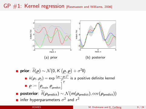
GP #1: Kernel regression [Rasmussen and Williams, 2006]
C. E. Rasmussen & C. K. I. Williams, Gaussian Processes for Machine Learning, the MIT Press, 2006,ISBN 026218253X. c 2006 Massachusetts Institute of Technology. www.GaussianProcess.org/gpml
2.2 Function-space View 15
−5 0 5
−2
−1
0
1
2
input, x
outp
ut, f
(x)
−5 0 5
−2
−1
0
1
2
input, x
outp
ut, f
(x)
(a), prior (b), posterior
Figure 2.2: Panel (a) shows three functions drawn at random from a GP prior;the dots indicate values of y actually generated; the two other functions have (lesscorrectly) been drawn as lines by joining a large number of evaluated points. Panel (b)shows three random functions drawn from the posterior, i.e. the prior conditioned onthe five noise free observations indicated. In both plots the shaded area represents thepointwise mean plus and minus two times the standard deviation for each input value(corresponding to the 95% confidence region), for the prior and posterior respectively.
which informally can be thought of as roughly the distance you have to move ininput space before the function value can change significantly, see section 4.2.1.For eq. (2.16) the characteristic length-scale is around one unit. By replacing|xpxq| by |xpxq|/` in eq. (2.16) for some positive constant ` we could changethe characteristic length-scale of the process. Also, the overall variance of the magnitude
random function can be controlled by a positive pre-factor before the exp ineq. (2.16). We will discuss more about how such factors a↵ect the predictionsin section 2.3, and say more about how to set such scale parameters in chapter5.
Prediction with Noise-free Observations
We are usually not primarily interested in drawing random functions from theprior, but want to incorporate the knowledge that the training data providesabout the function. Initially, we will consider the simple special case where theobservations are noise free, that is we know (xi, fi)|i = 1, . . . , n. The joint joint prior
distribution of the training outputs, f , and the test outputs f according to theprior is
ff
N
0,
K(X, X) K(X, X)K(X, X) K(X, X)
. (2.18)
If there are n training points and n test points then K(X, X) denotes then n matrix of the covariances evaluated at all pairs of training and testpoints, and similarly for the other entries K(X, X), K(X, X) and K(X, X).To get the posterior distribution over functions we need to restrict this jointprior distribution to contain only those functions which agree with the observeddata points. Graphically in Figure 2.2 you may think of generating functionsfrom the prior, and rejecting the ones that disagree with the observations, al- graphical rejection
(a) prior
C. E. Rasmussen & C. K. I. Williams, Gaussian Processes for Machine Learning, the MIT Press, 2006,ISBN 026218253X. c 2006 Massachusetts Institute of Technology. www.GaussianProcess.org/gpml
2.2 Function-space View 15
−5 0 5
−2
−1
0
1
2
input, x
outp
ut, f
(x)
−5 0 5
−2
−1
0
1
2
input, x
outp
ut, f
(x)
(a), prior (b), posterior
Figure 2.2: Panel (a) shows three functions drawn at random from a GP prior;the dots indicate values of y actually generated; the two other functions have (lesscorrectly) been drawn as lines by joining a large number of evaluated points. Panel (b)shows three random functions drawn from the posterior, i.e. the prior conditioned onthe five noise free observations indicated. In both plots the shaded area represents thepointwise mean plus and minus two times the standard deviation for each input value(corresponding to the 95% confidence region), for the prior and posterior respectively.
which informally can be thought of as roughly the distance you have to move ininput space before the function value can change significantly, see section 4.2.1.For eq. (2.16) the characteristic length-scale is around one unit. By replacing|xpxq| by |xpxq|/` in eq. (2.16) for some positive constant ` we could changethe characteristic length-scale of the process. Also, the overall variance of the magnitude
random function can be controlled by a positive pre-factor before the exp ineq. (2.16). We will discuss more about how such factors a↵ect the predictionsin section 2.3, and say more about how to set such scale parameters in chapter5.
Prediction with Noise-free Observations
We are usually not primarily interested in drawing random functions from theprior, but want to incorporate the knowledge that the training data providesabout the function. Initially, we will consider the simple special case where theobservations are noise free, that is we know (xi, fi)|i = 1, . . . , n. The joint joint prior
distribution of the training outputs, f , and the test outputs f according to theprior is
ff
N
0,
K(X, X) K(X, X)K(X, X) K(X, X)
. (2.18)
If there are n training points and n test points then K(X, X) denotes then n matrix of the covariances evaluated at all pairs of training and testpoints, and similarly for the other entries K(X, X), K(X, X) and K(X, X).To get the posterior distribution over functions we need to restrict this jointprior distribution to contain only those functions which agree with the observeddata points. Graphically in Figure 2.2 you may think of generating functionsfrom the prior, and rejecting the ones that disagree with the observations, al- graphical rejection
(b) posterior
prior: δ(ρ) ∼ N (0,K(ρ,ρ
)+ σ2I)
k(ρi ,ρj) = exp‖ρi−ρj‖2
r2 is a positive definite kernel
ρ :=[ρ
trainρ
predict
]T
posterior: δ(ρpredict) ∼ N (m(ρpredict), cov(ρpredict))
infer hyperparameters σ2 and r 2
ROMES M. Drohmann and K. Carlberg 9 / 24
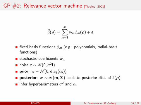
GP #2: Relevance vector machine [Tipping, 2001]
δ(ρ) =M∑
m=1
wmφm(ρ) + ε
fixed basis functions φm (e.g., polynomials, radial-basisfunctions)
stochastic coefficients wm
noise ε ∼ N (0, σ2I)
prior: w ∼ N (0, diag(αi ))
posterior: w ∼ N (m,Σ) leads to posterior dist. of δ(ρ)
infer hyperparameters σ2 and αi
ROMES M. Drohmann and K. Carlberg 10 / 24
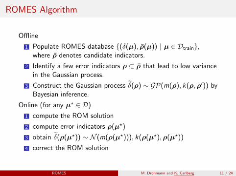
ROMES Algorithm
Offline
1 Populate ROMES database (δ(µ), ρ(µ)) | µ ∈ Dtrain,where ρ denotes candidate indicators.
2 Identify a few error indicators ρ ⊂ ρ that lead to low variancein the Gaussian process.
3 Construct the Gaussian process δ(ρ) ∼ GP(m(ρ), k(ρ,ρ′)) byBayesian inference.
Online (for any µ? ∈ D)
1 compute the ROM solution
2 compute error indicators ρ(µ?)
3 obtain δ(ρ(µ?)) ∼ N (m(ρ(µ?))), k(ρ(µ?),ρ(µ?))
4 correct the ROM solution
ROMES M. Drohmann and K. Carlberg 11 / 24
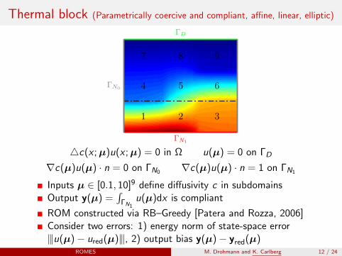
Thermal block (Parametrically coercive and compliant, affine, linear, elliptic)
1 2 3
4 5 6
7 8 9
ΓD
ΓN1
ΓN0
4c(x ;µ)u(x ;µ) = 0 in Ω u(µ) = 0 on ΓD
∇c(µ)u(µ) · n = 0 on ΓN0 ∇c(µ)u(µ) · n = 1 on ΓN1
Inputs µ ∈ [0.1, 10]9 define diffusivity c in subdomainsOutput y(µ) =
∫ΓN1
u(µ)dx is compliant
ROM constructed via RB–Greedy [Patera and Rozza, 2006]Consider two errors: 1) energy norm of state-space error|||u(µ)− ured(µ)|||, 2) output bias y(µ)− yred(µ)
ROMES M. Drohmann and K. Carlberg 12 / 24
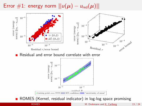
Error #1: energy norm |||u(µ)− ured(µ)|||
10−5 10−4
10−5
10−4
Residual r/error bound
error(energy
norm
)|||u
h−
ure
d|||
10−5
10−4
10−5
10−4
10−5
10−4
Residual r error b
ound
error(energy
norm
)|||u
h−
ure
d|||
(r; |||δu|||)(∆µ
u ; |||δu|||)
Residual and error bound correlate with error
105 104
105
104
residual R
erro
r(e
ner
gy
norm
)|||u
h
ure
d|||
(i) Kernel method
105 104
106
104
residual R
erro
r(e
ner
gy
norm
)|||u
h
ure
d|||
(ii) RVM
training point mean 95% confidence “uncertainty of mean”
105 104
105
104
residual R
erro
r(e
ner
gy
norm
)|||u
h
ure
d|||
(i) Kernel method
105 104
106
104
residual R
erro
r(e
ner
gy
norm
)|||u
h
ure
d|||
(ii) RVM
training point mean 95% confidence “uncertainty of mean”
ROMES (Kernel, residual indicator) in log-log space promisingROMES M. Drohmann and K. Carlberg 13 / 24
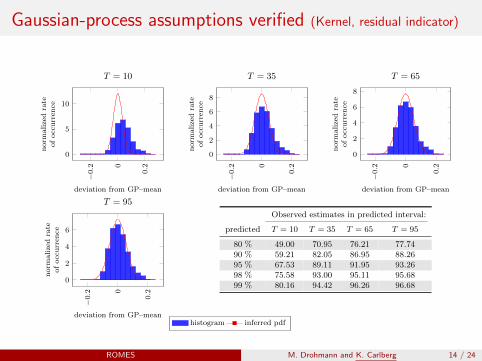
Gaussian-process assumptions verified (Kernel, residual indicator)
−0.2 0
0.2
0
5
10
deviation from GP–mean
norm
alizedrate
ofoccurren
ce
T = 10
−0.2 0
0.2
0
2
4
6
8
deviation from GP–meannorm
alizedrate
ofoccurren
ce
T = 35
−0.2 0
0.2
0
2
4
6
8
deviation from GP–mean
norm
alizedrate
ofoccurren
ce
T = 65−0.2 0
0.2
0
2
4
6
deviation from GP–mean
norm
alizedrate
ofoccurren
ce
T = 95
Observed estimates in predicted interval:
predicted T = 10 T = 35 T = 65 T = 95
80 % 49.00 70.95 76.21 77.7490 % 59.21 82.05 86.95 88.2695 % 67.53 89.11 91.95 93.2698 % 75.58 93.00 95.11 95.6899 % 80.16 94.42 96.26 96.68
histogram inferred pdf
ROMES M. Drohmann and K. Carlberg 14 / 24
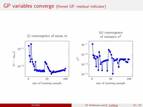
GP variables converge (Kernel GP, residual indicator)
0 50 100
10−2
10−1
size of training sample
‖ν−
νfi
ne‖
(i) convergence of mean m
0 50 100
10−4
10−3
10−2
10−1
size of training sample
σ2
(ii) convergenceof variance σ2
ROMES M. Drohmann and K. Carlberg 15 / 24
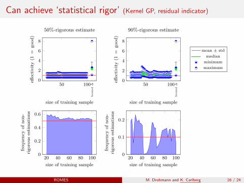
Can achieve ‘statistical rigor’ (Kernel GP, residual indicator)
50 1000
2
4
6
8
bound
∆
size of training sample
effec
tivit
y(1
=good
)50%-rigorous estimate
50 1000
2
4
6
8
bound
∆
size of training sample
effec
tivit
y(1
=good
)
90%-rigorous estimate
20 40 60 80 1000
0.2
0.4
0.6
size of training sample
freq
uen
cyof
non
-ri
goro
us
esti
mati
on
s
20 40 60 80 1000
0.1
0.2
size of training sample
freq
uen
cyof
non
-ri
goro
us
esti
mati
on
s
mean ± std
median
minimum
maximum
ROMES M. Drohmann and K. Carlberg 16 / 24
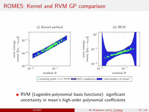
ROMES: Kernel and RVM GP comparison
10−2 10−110−3
10−2
10−1
residual R
error(energy
norm
)|||u
h−
ure
d|||
(i) Kernel method
10−2 10−1
10−3
10−1
101
residual R
error(energy
norm
)|||u
h−
ure
d|||
(ii) RVM
training point mean 95% confidence “uncertainty of mean”
RVM (Legendre-polynomial basis functions): significantuncertainty in mean’s high-order polynomial coefficients
ROMES M. Drohmann and K. Carlberg 17 / 24
ROMES: Kernel and RVM GP comparison
0.2 0
0.2
0
2
4
6
8
deviation from GP–mean
norm
alize
dra
teofocc
urr
ence
(i) Kernel method
0.5 0
0.5
0
0.5
1
1.5
deviation from GP–mean
norm
alize
dra
teofocc
urr
ence
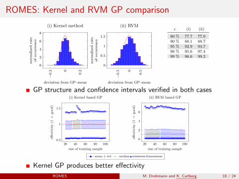
(ii) RVMObserved estimates in c–confidence interval of normaldistribution with variance
2 2 + diag()
c (i) (ii) (i) (ii)
80 % 77.7 77.9 84.32 92.7490 % 88.1 88.7 92.53 97.7995 % 92.9 94.7 95.11 99.7498 % 95.6 97.4 97.11 100.0099 % 96.6 99.2 98.53 100.00
histogram inferred pdf
0.2 0
0.2
0
2
4
6
8
deviation from GP–mean
norm
alize
dra
teofocc
urr
ence
(i) Kernel method
0.5 0
0.5
0
0.5
1
1.5
deviation from GP–mean
norm
alize
dra
teofocc
urr
ence
(ii) RVMObserved estimates in c–confidence interval of normaldistribution with variance
2 2 + diag()
c (i) (ii) (i) (ii)
80 % 77.7 77.9 84.32 92.7490 % 88.1 88.7 92.53 97.7995 % 92.9 94.7 95.11 99.7498 % 95.6 97.4 97.11 100.0099 % 96.6 99.2 98.53 100.00
histogram inferred pdf
GP structure and confidence intervals verified in both cases
20 40 60 80 1000.5
1
1.5
size of training sample
effec
tivit
y(1
=good
)
(i) Kernel based GP
20 40 60 80 100
0
2
4
6
size of training sample
effec
tivit
y(1
=good
)
(ii) RVM based GP
mean ± std median minimum maximum
Kernel GP produces better effectivity
ROMES M. Drohmann and K. Carlberg 18 / 24
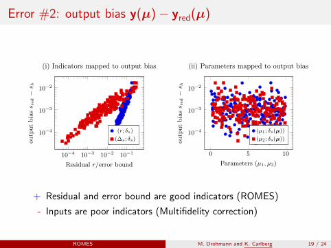
Error #2: output bias y(µ)− yred(µ)
10−4 10−3 10−2 10−1
10−4
10−3
10−2
Residual r/error bound
outputbiass r
ed−s h
(i) Indicators mapped to output bias
0 5 10
10−4
10−3
10−2
Parameters (µ1, µ2)
outputbiass r
ed−s h
(ii) Parameters mapped to output bias
(r; δs)
(∆s; δs)
(µ1; δs(µ))
(µ2; δs(µ))
+ Residual and error bound are good indicators (ROMES)
- Inputs are poor indicators (Multifidelity correction)
ROMES M. Drohmann and K. Carlberg 19 / 24
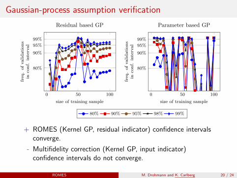
Gaussian-process assumption verification
0 50 100
80%
90%
95%
99%
size of training sample
freq
.ofvalidations
inco
nf.
interval
Residual based GP
0 50 100
80%
90%
95%
99%
size of training sample
freq
.ofvalidations
inco
nf.
interval
Parameter based GP
80% 90% 95% 98% 99%
+ ROMES (Kernel GP, residual indicator) confidence intervalsconverge.
- Multifidelity correction (Kernel GP, input indicator)confidence intervals do not converge.
ROMES M. Drohmann and K. Carlberg 20 / 24
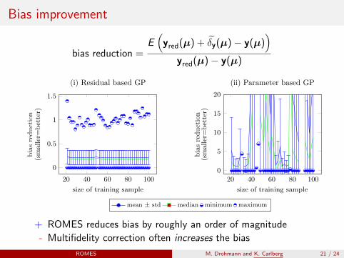
Bias improvement
bias reduction =E(
yred(µ) + δy(µ)− y(µ))
yred(µ)− y(µ)
20 40 60 80 100
0
0.5
1
1.5
size of training sample
impro
vem
ent
(sm
aller
=bet
ter)
(i) Residual based GP
20 40 60 80 100
0
5
10
15
20
size of training sampleim
pro
vem
ent
(sm
aller
=bet
ter)
(ii) Parameter based GP
mean ± std median minimum maximum
bia
sre
duct
ion
bia
sre
duct
ion
+ ROMES reduces bias by roughly an order of magnitude
- Multifidelity correction often increases the bias
ROMES M. Drohmann and K. Carlberg 21 / 24
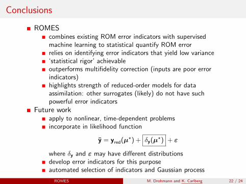
Conclusions
ROMEScombines existing ROM error indicators with supervisedmachine learning to statistical quantify ROM errorrelies on identifying error indicators that yield low variance‘statistical rigor’ achievableoutperforms multifidelity correction (inputs are poor errorindicators)highlights strength of reduced-order models for dataassimilation: other surrogates (likely) do not have suchpowerful error indicators
Future workapply to nonlinear, time-dependent problemsincorporate in likelihood function
y = yred(µ?) + δy(µ?) + ε
where δy and ε may have different distributionsdevelop error indicators for this purposeautomated selection of indicators and Gaussian process
ROMES M. Drohmann and K. Carlberg 22 / 24

Acknowledgments
Khachik Sargsyan: helpful discussions
This research was supported in part by an appointment to theSandia National Laboratories Truman Fellowship in NationalSecurity Science and Engineering, sponsored by SandiaCorporation (a wholly owned subsidiary of Lockheed MartinCorporation) as Operator of Sandia National Laboratoriesunder its U.S. Department of Energy Contract No.DE-AC04-94AL85000.
ROMES M. Drohmann and K. Carlberg 23 / 24
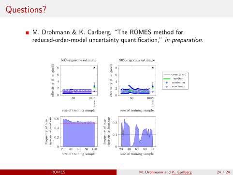
Questions?
M. Drohmann & K. Carlberg, “The ROMES method forreduced-order-model uncertainty quantification,” in preparation.
50 1000
2
4
6
8
bound
∆
size of training sample
effec
tivit
y(1
=good)
50%-rigorous estimate
50 1000
2
4
6
8
bound
∆
size of training sampleeff
ecti
vit
y(1
=good)
90%-rigorous estimate
20 40 60 80 1000
0.2
0.4
0.6
size of training sample
freq
uen
cyof
non-
rigoro
us
esti
mati
ons
20 40 60 80 1000
0.1
0.2
size of training sample
freq
uen
cyof
non-
rigoro
us
esti
mati
ons
mean ± std
median
minimum
maximum
ROMES M. Drohmann and K. Carlberg 24 / 24
Bibliography I
Eldred, M. S., Giunta, A. A., Collis, S. S., Alexandrov, N. A.,and Lewis, R. M. (2004).Second-order corrections for surrogate-based optimization withmodel hierarchies.In Proceedings of the 10th AIAA/ISSMO MultidisciplinaryAnalysis and Optimization Conference, Albany, NY, numberAIAA Paper 2004-4457.
Galbally, D., Fidkowski, K., Willcox, K., and Ghattas, O.(2009).Non-linear model reduction for uncertainty quantification inlarge-scale inverse problems.International Journal for Numerical Methods in Engineering,81(12):1581–1608.
ROMES M. Drohmann and K. Carlberg 25 / 24
Bibliography II
Huynh, D. B. P., Knezevic, D. J., Chen, Y., Hesthaven, J. S.,and Patera, A. T. (2010).A natural-norm successive constraint method for inf-sup lowerbounds.Comput. Methods Appl. Mech. Engrg., 199:1963–1975.
Ng, L. and Eldred, M. S. (2012).Multifidelity uncertainty quantification using non-intrusivepolynomial chaos and stochastic collocation.In AIAA 2012-1852.
Patera, A. T. and Rozza, G. (2006).Reduced basis approximation and a posteriori error estimationfor parametrized partial differential equations.MIT.
ROMES M. Drohmann and K. Carlberg 26 / 24
Bibliography III
Rasmussen, C. and Williams, C. (2006).Gaussian Processes for Machine Learning.MIT Press.
Tipping, M. E. (2001).Sparse bayesian learning and the relevance vector machine.The Journal of Machine Learning Research, 1:211–244.
Wirtz, D., Sorensen, D. C., and Haasdonk, B. (2012).A-posteriori error estimation for DEIM reduced nonlineardynamical systems.Preprint Series, Stuttgart Research Centre for SimulationTechnology.
ROMES M. Drohmann and K. Carlberg 27 / 24
Bibliography IV
Yano, M., Patera, A. T., and Urban, K. (2012).A space-time certified reduced-basis method for Burgers’equation.Math. Mod. Meth. Appl. S., submitted.
ROMES M. Drohmann and K. Carlberg 28 / 24