The role of two interest rates in the intertemporalcurrent account model∗

MichaÃl Rubaszek†

This draft, March 2010

Abstract

The paper analyses the role of the lending-deposit interest rate spread in thedynamics of the current account in developing countries. For that purpose weextend the standard perfect-foresight intertemporal model of the current accountfor the existence of the interest rate spread and simulate the convergence pathof developing economies. This model helps explain why in many cases it is op-timal for a fast growing, low income countries to run balanced current account.Our theoretical considerations are confirmed by the panel data for 60 developingcountries, which points to a significant relationship between the current accountand the interest rate spread.

Keywords: Intertemporal current account; financial market imperfections; eco-nomic convergenceJEL Classification: C32; F12; F31.

∗I’m grateful to Michele Ca’Zorzi and Marcin Kolasa for lengthy discussions that highly contributedto the final version of this article. I also thank MichaÃl Gradzewicz, Jakub Growiec and RyszardKokoszczynski for valuable comments and suggestions. Previous versions of this paper were presentedat the First International Symposium in Computational Economics and Finance (Sousse, 2010), theNational Bank of Poland (Warsaw, 2010) and the Warsaw School of Economics (Warsaw, 2010).

†National Bank of Poland and Warsaw School of Economics. E-mail: michal.rubaszek@nbp.pl

1

1 Introduction

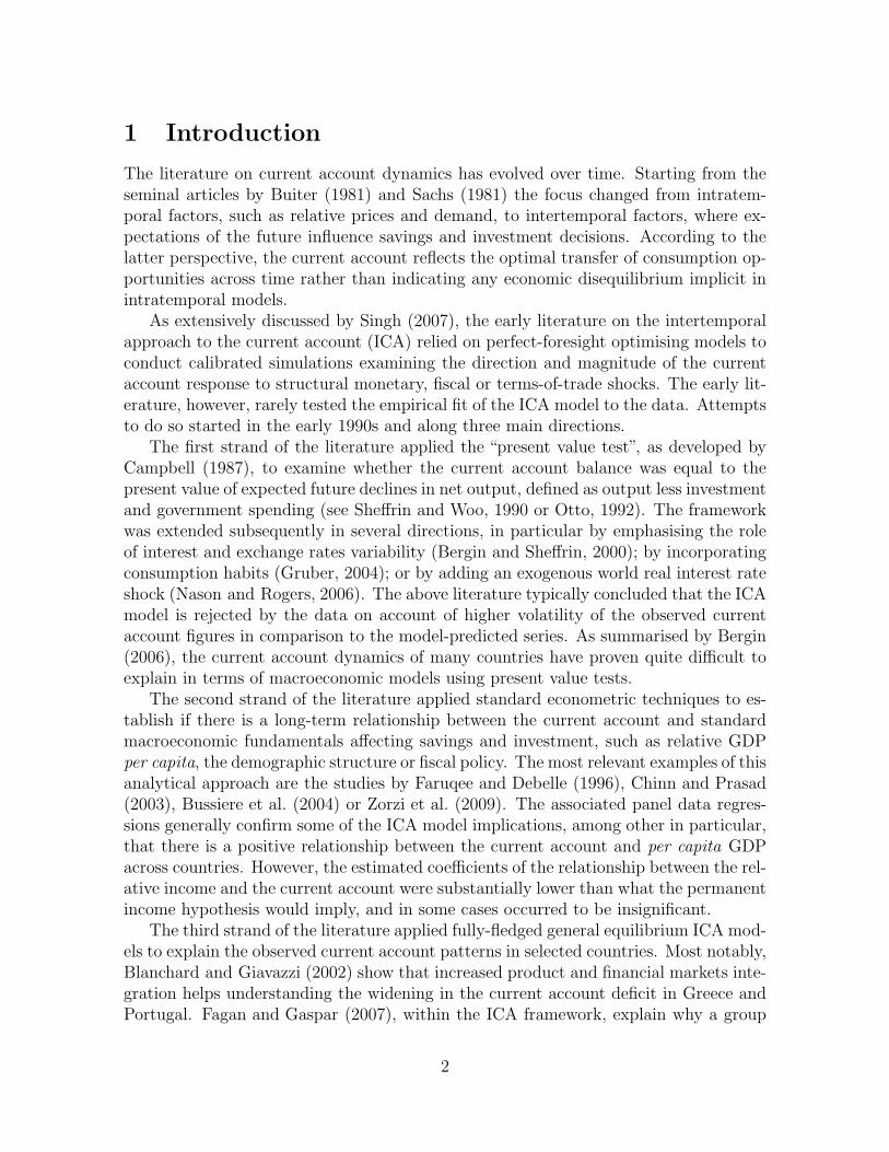
The literature on current account dynamics has evolved over time. Starting from theseminal articles by Buiter (1981) and Sachs (1981) the focus changed from intratem-poral factors, such as relative prices and demand, to intertemporal factors, where ex-pectations of the future influence savings and investment decisions. According to thelatter perspective, the current account reflects the optimal transfer of consumption op-portunities across time rather than indicating any economic disequilibrium implicit inintratemporal models.

As extensively discussed by Singh (2007), the early literature on the intertemporalapproach to the current account (ICA) relied on perfect-foresight optimising models toconduct calibrated simulations examining the direction and magnitude of the currentaccount response to structural monetary, fiscal or terms-of-trade shocks. The early lit-erature, however, rarely tested the empirical fit of the ICA model to the data. Attemptsto do so started in the early 1990s and along three main directions.

The first strand of the literature applied the “present value test”, as developed byCampbell (1987), to examine whether the current account balance was equal to thepresent value of expected future declines in net output, defined as output less investmentand government spending (see Sheffrin and Woo, 1990 or Otto, 1992). The frameworkwas extended subsequently in several directions, in particular by emphasising the roleof interest and exchange rates variability (Bergin and Sheffrin, 2000); by incorporatingconsumption habits (Gruber, 2004); or by adding an exogenous world real interest rateshock (Nason and Rogers, 2006). The above literature typically concluded that the ICAmodel is rejected by the data on account of higher volatility of the observed currentaccount figures in comparison to the model-predicted series. As summarised by Bergin(2006), the current account dynamics of many countries have proven quite difficult toexplain in terms of macroeconomic models using present value tests.

The second strand of the literature applied standard econometric techniques to es-tablish if there is a long-term relationship between the current account and standardmacroeconomic fundamentals affecting savings and investment, such as relative GDPper capita, the demographic structure or fiscal policy. The most relevant examples of thisanalytical approach are the studies by Faruqee and Debelle (1996), Chinn and Prasad(2003), Bussiere et al. (2004) or Zorzi et al. (2009). The associated panel data regres-sions generally confirm some of the ICA model implications, among other in particular,that there is a positive relationship between the current account and per capita GDPacross countries. However, the estimated coefficients of the relationship between the rel-ative income and the current account were substantially lower than what the permanentincome hypothesis would imply, and in some cases occurred to be insignificant.

The third strand of the literature applied fully-fledged general equilibrium ICA mod-els to explain the observed current account patterns in selected countries. Most notably,Blanchard and Giavazzi (2002) show that increased product and financial markets inte-gration helps understanding the widening in the current account deficit in Greece andPortugal. Fagan and Gaspar (2007), within the ICA framework, explain why a group

2

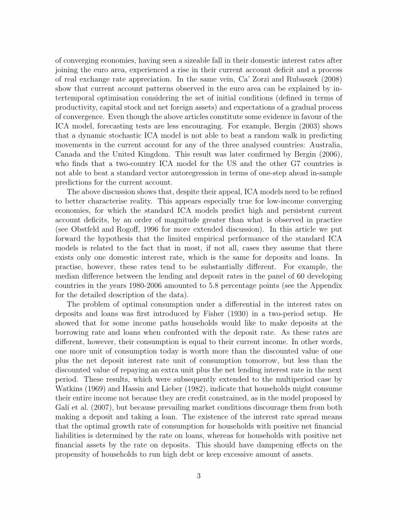
of converging economies, having seen a sizeable fall in their domestic interest rates afterjoining the euro area, experienced a rise in their current account deficit and a processof real exchange rate appreciation. In the same vein, Ca’ Zorzi and Rubaszek (2008)show that current account patterns observed in the euro area can be explained by in-tertemporal optimisation considering the set of initial conditions (defined in terms ofproductivity, capital stock and net foreign assets) and expectations of a gradual processof convergence. Even though the above articles constitute some evidence in favour of theICA model, forecasting tests are less encouraging. For example, Bergin (2003) showsthat a dynamic stochastic ICA model is not able to beat a random walk in predictingmovements in the current account for any of the three analysed countries: Australia,Canada and the United Kingdom. This result was later confirmed by Bergin (2006),who finds that a two-country ICA model for the US and the other G7 countries isnot able to beat a standard vector autoregression in terms of one-step ahead in-samplepredictions for the current account.

The above discussion shows that, despite their appeal, ICA models need to be refinedto better characterise reality. This appears especially true for low-income convergingeconomies, for which the standard ICA models predict high and persistent currentaccount deficits, by an order of magnitude greater than what is observed in practice(see Obstfeld and Rogoff, 1996 for more extended discussion). In this article we putforward the hypothesis that the limited empirical performance of the standard ICAmodels is related to the fact that in most, if not all, cases they assume that thereexists only one domestic interest rate, which is the same for deposits and loans. Inpractise, however, these rates tend to be substantially different. For example, themedian difference between the lending and deposit rates in the panel of 60 developingcountries in the years 1980-2006 amounted to 5.8 percentage points (see the Appendixfor the detailed description of the data).

The problem of optimal consumption under a differential in the interest rates ondeposits and loans was first introduced by Fisher (1930) in a two-period setup. Heshowed that for some income paths households would like to make deposits at theborrowing rate and loans when confronted with the deposit rate. As these rates aredifferent, however, their consumption is equal to their current income. In other words,one more unit of consumption today is worth more than the discounted value of oneplus the net deposit interest rate unit of consumption tomorrow, but less than thediscounted value of repaying an extra unit plus the net lending interest rate in the nextperiod. These results, which were subsequently extended to the multiperiod case byWatkins (1969) and Hassin and Lieber (1982), indicate that households might consumetheir entire income not because they are credit constrained, as in the model proposed byGalı et al. (2007), but because prevailing market conditions discourage them from bothmaking a deposit and taking a loan. The existence of the interest rate spread meansthat the optimal growth rate of consumption for households with positive net financialliabilities is determined by the rate on loans, whereas for households with positive netfinancial assets by the rate on deposits. This should have dampening effects on thepropensity of households to run high debt or keep excessive amount of assets.

3

At the country level, the existence of the interest rate spread can explain why low-income, converging economies are typically not running high current account deficits,leading to a sizeable build-up of foreign debt, as it is implied by the standard ICA model.Even though households would like to smooth their consumption on account of expectedgrowth in income, the high intertemporal price of future consumption, which is givenby the lending rate, constraints them from doing so and as a result their consumptionfollows closely their income.

So far these considerations have been ignored in the ICA literature. One reasonmight be of technical nature: in an environment with a different rate on assets anddebt, the relation between net financial position of households and the interest rate isnot continuous around the steady state. Consequently, the standard perturbation tech-niques of solving dynamic general equilibrium models cannot be applied in this setting.We tackle this problem by using numerical, direct optimisation methods. However, dueto the fact that the perturbation techniques cannot be applied in our framework, welimit our analysis to the perfect-foresight framework, leaving for further research torelax the one-interest assumption in a stochastic ICA model.

The main contribution of this paper is twofold. First, we show that due to theexistence of the interest rate spread it might be optimal for low-income, convergingeconomies to run balanced current accounts. Moreover, we indicate that for small val-ues of the spread its further narrowing can have very substantial effects on savings andinvestment decisions, hence on the level of the current account. Second, on the basisof the panel for 60 developing countries we provide empirical evidence of our theoreti-cal model implications by showing that there is a significant relationship between thecurrent account balance and the lending-deposit interest rate spread.

The article is structured as follows. The next two sections present the ICA modeland the method of solving it. Section 4 presents simulation results, which show thatin the environment of two interest rates the model implied current account deficits oflow-income converging economies is substantially lower what the standard ICA modelwould imply. Finally, Section 5 presents empirical evidence on the relationship betweenthe interest spread and the current account, where the data used for estimation aredescribed in the Appendix. The last section concludes.

2 The model

The model economy is populated by representative households that are both consumersand producers. The following additional features are included. The model economy issmall open and subject to a convergence process. There is a banking sector, whichdifferentiates between a lending and a deposit rates. There are adjustment costs asso-ciated to the accumulation of capital. In the exposition of the model, which presentedbelow, we use lower-case letters for individual variables, whereas capital letters standfor country aggregates.

4

2.1 Households

The model economy is populated by a continuum of identical household-producers max-imising their utility from consumption ct:

max U0 =T∑

t=0

βtu(ct), (1)

and producing output yt according to the Cobb-Douglas technology:

yt = kαt Z1−α

t . (2)

Here kt is per household level of capital available at the beginning of period t and Zt

stands for the home country level of productivity. Produced output can be invested incapital, deposited in a bank or consumed. The capital stock evolves in line with thefollowing equation:

kt+1 = (1− δ)kt + it(1− ψκt), (3)

where it is investment expenditures, δ the depreciation rate and ψ capital adjustmentcost parameter. The variable κt is the individual investment-capital ratio relative toits steady-state value IK∗, κt = it/kt

IK∗ , where “∗” stands for foreign economy that isassumed to be permanently in the steady state (a similar assumption was done byCa’ Zorzi and Rubaszek, 2008). The above specification means that the capital is ac-cumulated subject to adjustment costs, introduced in vein of the framework proposedby Hayashi (1982), so that only a fraction of investment turns into capital.

Households can participate in financial markets through banks, which offer loansand deposits at gross rates RL

t and RAt . Finally, consumption is taxed at rate τ . As a

result, the representative household faces the following budget constraint:

at+1 − lt+1 = RAt at −RL

t lt + yt − it − (1 + τ)ct, (4)

where at ≥ 0 and lt ≥ 0 are household assets and liabilities at the beginning of periodt.

2.2 Banks

The banking sector consists of a continuum of identical banks that are maximisingprofits from loans and deposits. Profits are due to the fact that the deposit interestrate rA

t set by the bank is lower than its borrowing rate rLt . The difference between

collected deposits and granted loans is covered by the participation in the interbankmarket, where funds can be raised or deposited at rate Rt. As a result, profits equal to:

πt =(rLt −Rt

)lbt + (Rt − rA

t )abt , (5)

5

where lbt and abt stand for loans granted and deposits collected by the bank. For the

sake of simplicity we abstract from any risk considerations or fixed costs incurred bybanks. Instead, we assume that deposit and loan interest rates differ from the interbankrate due to the monopolistic power of each bank in the market. The implementationof the monopolistic competition framework proposed by Gerali et al. (2009) yields thefollowing demand equations for loans and deposits:

lbankt =

(rLt

RLt

)−θL

Lt (6)

abankt =

(rAt

RAt

)θA

At, (7)

where θL and θA are demand elasticities for loans and deposits, respectively. Themaximisation of (5) subject to (6) and (7) sets the level of the interest rates at rL

t =θL

θL−1Rt and rA

t = θA

θA+1Rt. As all banks are assumed to be identical, the country-wide

level of the rates is RLt = rL

t and RAt = rA

t .

2.3 Closing the model and the current account

To close the model we assume that the government is passive and runs a balancedbudget, i.e. tax revenues are spent in the form of public expenditures (Gt):

Gt = τCt. (8)

Subsequently, we assume that the country’s productivity is converging to its steady-state path Z∗

t , which is growing at a deterministic rate γ, at pace ρ:

Zt = ρZt−1 + (1− ρ)Z∗t . (9)

Finally, we set the interbank interest rate at the level of global interest rate (R∗), whichis assumed to be constant:

Rt = R∗. (10)

The current account is calculated as the increment in the stock of net foreign assets,i.e.:

CAt = (At+1 − Lt+1)− (At − Lt) , (11)

where changes in aggregate assets and liabilities are given by:

At+1 − Lt+1 = RAt At −RL

t Lt + Yt − Ct − It −Gt. (12)

It should be noted that in this setting we assume that banks are foreign owned andprofits of the banking sector are transferred abroad. This assumption broadly reflectsthe situation in most developing countries, which are the main focus of this article.

6

3 Solving the model

We solve the model by using numerical techniques. For that purpose, we write theoptimisation problem faced by households in a finite-horizon setting, where we set largevalues of the last period T ,1, which enables us to extrapolate our findings for infinitehorizon. Households maximise their utility, given by (1), by choosing the sequence ofct, it, at+1, lt+1 and implicitly kt+1 that satisfy equality constraints (2), (3) and (4),nonnegativity conditions at ≥ 0 and lt ≥ 0, terminal conditions aT+1 = 0, lT+1 = 0and kT+1 = K∗

T+1, given the initial values a0, l0 and k0. As a result, the Lagrangeanfunction takes the form:

L =∑T

t=0{βtu(ct) + λt[RAt at −RL

t lt + kαt Z1−α

t − it − (1 + τ)ct − at+1 + lt+1]+ qt[(1− δ)kt + it(1− ψκt)− kt+1] + µA

t at+1 + µLt lt+1}

+ νAaT+1 + νLlT+1 + νK(kT+1 −K∗T+1) + ωAa0 + ωLl0 + ωKk0

(13)The respective Karush-Kuhn-Tucker (KKT) first order conditions for this problem aregiven by:

ct : λt =βt

1− τu′(ct) (14)

at+1 : λt = RAt+1λt+1 + µA

t (15)

lt+1 : λt = RLt+1λt+1 − µL

t (16)

it : λt = qt(1− 2ψκt) (17)

kt+1 : qt = λt+1α(kt+1Z

−1t+1

)α−1+ qt+1

[(1− δ) + ψκ2

t+1IK∗] (18)

Equation (14) defines the present value of the marginal utility from consumption, whichaccording to equations (15) and (16) is decreasing at a gross rate lying in the interval[RA

t ; RLt ]. It can be noticed that if at+1 > 0 then the decrease rate is equal to RA

t andif lt+1 > 0 then it amounts to RL

t as the KKT complementarily conditions state thatµA

t at+1 = 0 and µLt lt+1 = 0. Equation (17) relates the market value of capital, i.e.

q-Tobin ratio, to marginal utility of consumption. Finally, equation (18) determinesthe dynamics of the capital shadow price.

4 The results

This section presents the results of a number of simulations showing the convergencepath of the model economy, focusing on the role of the initial conditions and the interestrate spread. We start by discussing the parameterisation of the model and the resulting

1We define large values of T as the values for which current account balance and net foreign assetsin the last few periods of simulation are null.

7

steady-state path. Then, we elaborate on the relationship between GDP per capita,initial stock of capital, the interest rate spread and the current account. Finally, weperform sensitivity analysis with respect to model parameterisation.

4.1 Parameterisation

The model economy is calibrated at an annual frequency. Since the structure of theeconomy is assumed to be the same at home and abroad, the corresponding parametersare also the same. All parameters, but convergence pace, are chosen to reflect valuesfor industrial countries and generally correspond to those by Ca’ Zorzi and Rubaszek(2008), who provide a thorough discussion of their choice.

The utility function is chosen to be logarithmic, u(ct) = ln ct, but the general find-ings presented below would still hold for a general class of concave and differentiablefunctions. The steady-state growth rate of productivity γ is set to 1.5 percent per yearand the discount factor β to 0.975, which implies that steady-state real interest rateR∗ is around 1.04. The coefficient ψ is fixed at 0.10, so that in the steady state 10%of investments covers installation costs (see Roeger and in ’t Veld, 2004). The depre-ciation rate δ is chosen to be 0.08 and the share of capital α is 0.30, which impliesthe steady-state investment and capital-output ratios at 0.23 and 2.19, respectively.2

The tax rate τ is fixed at 0.33, so that private consumption and government spendingconstitute 58 and 19 percent of GDP.

For the remaining parameters, determining the convergence path to the steady state,we fixed the convergence pace ρ at 0.95, so that the half-life of productivity gap amountsto around thirteen years. This assumption is clearly more optimistic than the literatureconsensus of around 0.98, but we decided to take this value to show that even highspeed of convergence might not be sufficient to generate a current account deficit in theenvironment of high interest rate spread. The demand elasticity for deposits θA andloans θL is set to 50, so that the lending-deposit rates spread was around a reasonablevalue of 4 percentage points.

4.2 Simulating convergence path

The first simulation investigates the convergence path of the model economy for differentassumptions concerning the initial level of GDP per capita. We analyse four cases inwhich the initial output is equal to one quarter, one third, one half and three quartersof its steady-state value. We assume that the starting value of the capital-output ratiois equal to its steady-state value, KY0 = KY ∗, and that net foreign assets are null,B0 = 0. These additional assumptions are helpful in isolating the impact of the interestrate spread on the current account dynamics in converging economies. However, we willrelax them later, considering that developing countries are generally characterised by

2The steady-state investment-capital ratio equals to IK∗ = γ+δ1−ψ and the capital-output ratio is

KY ∗ = α(1−2ψ)R∗+δ−1−ψIK∗

8

lower capital-output ratios (see Nehru and Dhareshwar, 1993) than industrial countriesand run positive net foreign debt (see Lane and Milesi-Ferretti, 2001).

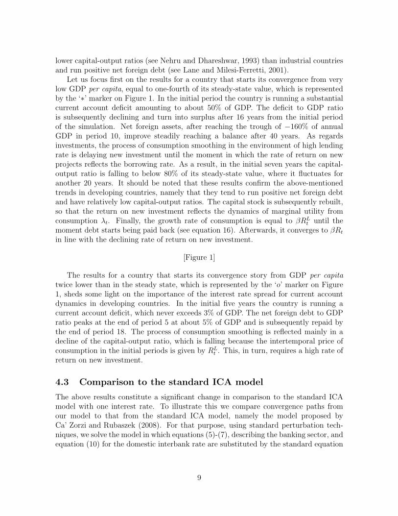
Let us focus first on the results for a country that starts its convergence from verylow GDP per capita, equal to one-fourth of its steady-state value, which is representedby the ‘∗’ marker on Figure 1. In the initial period the country is running a substantialcurrent account deficit amounting to about 50% of GDP. The deficit to GDP ratiois subsequently declining and turn into surplus after 16 years from the initial periodof the simulation. Net foreign assets, after reaching the trough of −160% of annualGDP in period 10, improve steadily reaching a balance after 40 years. As regardsinvestments, the process of consumption smoothing in the environment of high lendingrate is delaying new investment until the moment in which the rate of return on newprojects reflects the borrowing rate. As a result, in the initial seven years the capital-output ratio is falling to below 80% of its steady-state value, where it fluctuates foranother 20 years. It should be noted that these results confirm the above-mentionedtrends in developing countries, namely that they tend to run positive net foreign debtand have relatively low capital-output ratios. The capital stock is subsequently rebuilt,so that the return on new investment reflects the dynamics of marginal utility fromconsumption λt. Finally, the growth rate of consumption is equal to βRL

t until themoment debt starts being paid back (see equation 16). Afterwards, it converges to βRt

in line with the declining rate of return on new investment.

[Figure 1]

The results for a country that starts its convergence story from GDP per capitatwice lower than in the steady state, which is represented by the ‘o’ marker on Figure1, sheds some light on the importance of the interest rate spread for current accountdynamics in developing countries. In the initial five years the country is running acurrent account deficit, which never exceeds 3% of GDP. The net foreign debt to GDPratio peaks at the end of period 5 at about 5% of GDP and is subsequently repaid bythe end of period 18. The process of consumption smoothing is reflected mainly in adecline of the capital-output ratio, which is falling because the intertemporal price ofconsumption in the initial periods is given by RL

t . This, in turn, requires a high rate ofreturn on new investment.

4.3 Comparison to the standard ICA model

The above results constitute a significant change in comparison to the standard ICAmodel with one interest rate. To illustrate this we compare convergence paths fromour model to that from the standard ICA model, namely the model proposed byCa’ Zorzi and Rubaszek (2008). For that purpose, using standard perturbation tech-niques, we solve the model in which equations (5)-(7), describing the banking sector, andequation (10) for the domestic interbank rate are substituted by the standard equation

9

of new open economy models with market imperfections (Benigno, 2009):3

RLt = RA

t = Rt = R∗ exp(−φBt

Yt−1

) (19)

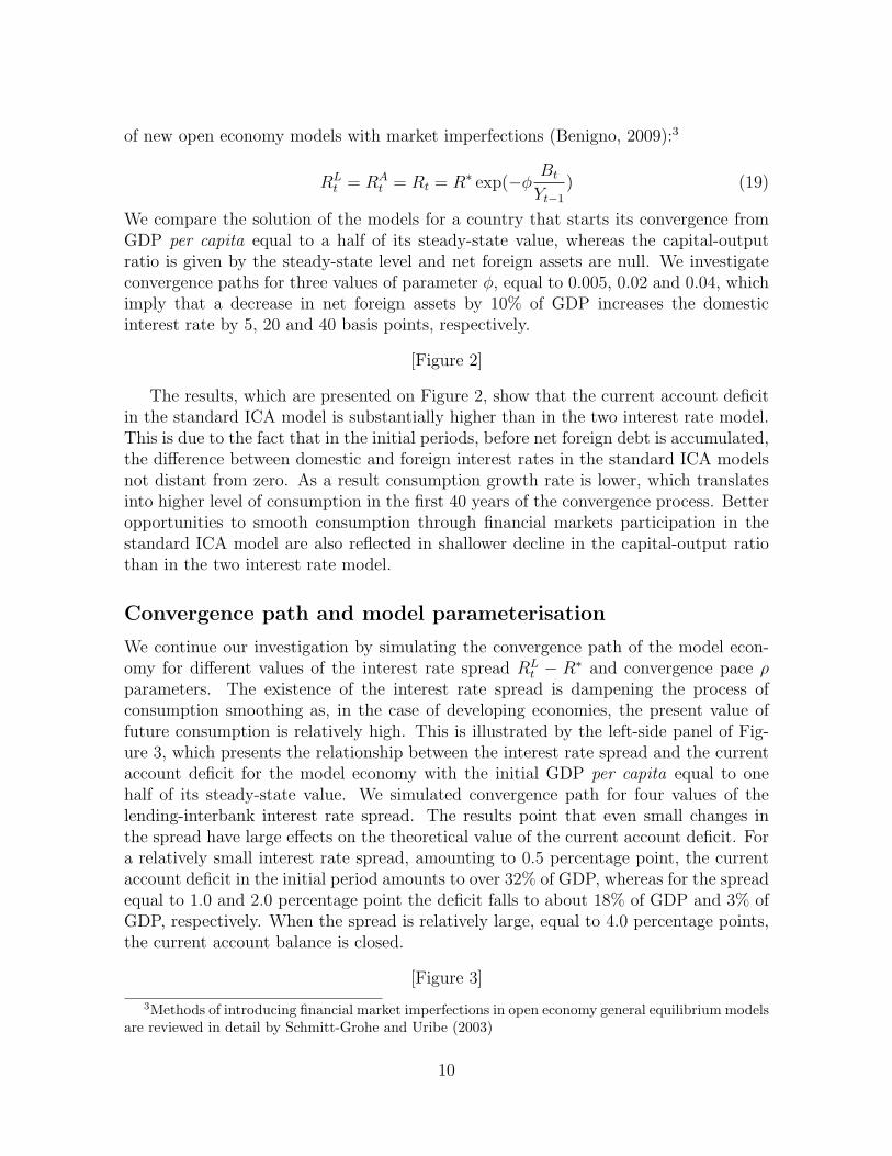
We compare the solution of the models for a country that starts its convergence fromGDP per capita equal to a half of its steady-state value, whereas the capital-outputratio is given by the steady-state level and net foreign assets are null. We investigateconvergence paths for three values of parameter φ, equal to 0.005, 0.02 and 0.04, whichimply that a decrease in net foreign assets by 10% of GDP increases the domesticinterest rate by 5, 20 and 40 basis points, respectively.

[Figure 2]

The results, which are presented on Figure 2, show that the current account deficitin the standard ICA model is substantially higher than in the two interest rate model.This is due to the fact that in the initial periods, before net foreign debt is accumulated,the difference between domestic and foreign interest rates in the standard ICA modelsnot distant from zero. As a result consumption growth rate is lower, which translatesinto higher level of consumption in the first 40 years of the convergence process. Betteropportunities to smooth consumption through financial markets participation in thestandard ICA model are also reflected in shallower decline in the capital-output ratiothan in the two interest rate model.

Convergence path and model parameterisation

We continue our investigation by simulating the convergence path of the model econ-omy for different values of the interest rate spread RL

t − R∗ and convergence pace ρparameters. The existence of the interest rate spread is dampening the process ofconsumption smoothing as, in the case of developing economies, the present value offuture consumption is relatively high. This is illustrated by the left-side panel of Fig-ure 3, which presents the relationship between the interest rate spread and the currentaccount deficit for the model economy with the initial GDP per capita equal to onehalf of its steady-state value. We simulated convergence path for four values of thelending-interbank interest rate spread. The results point that even small changes inthe spread have large effects on the theoretical value of the current account deficit. Fora relatively small interest rate spread, amounting to 0.5 percentage point, the currentaccount deficit in the initial period amounts to over 32% of GDP, whereas for the spreadequal to 1.0 and 2.0 percentage point the deficit falls to about 18% of GDP and 3% ofGDP, respectively. When the spread is relatively large, equal to 4.0 percentage points,the current account balance is closed.

[Figure 3]

3Methods of introducing financial market imperfections in open economy general equilibrium modelsare reviewed in detail by Schmitt-Grohe and Uribe (2003)

10

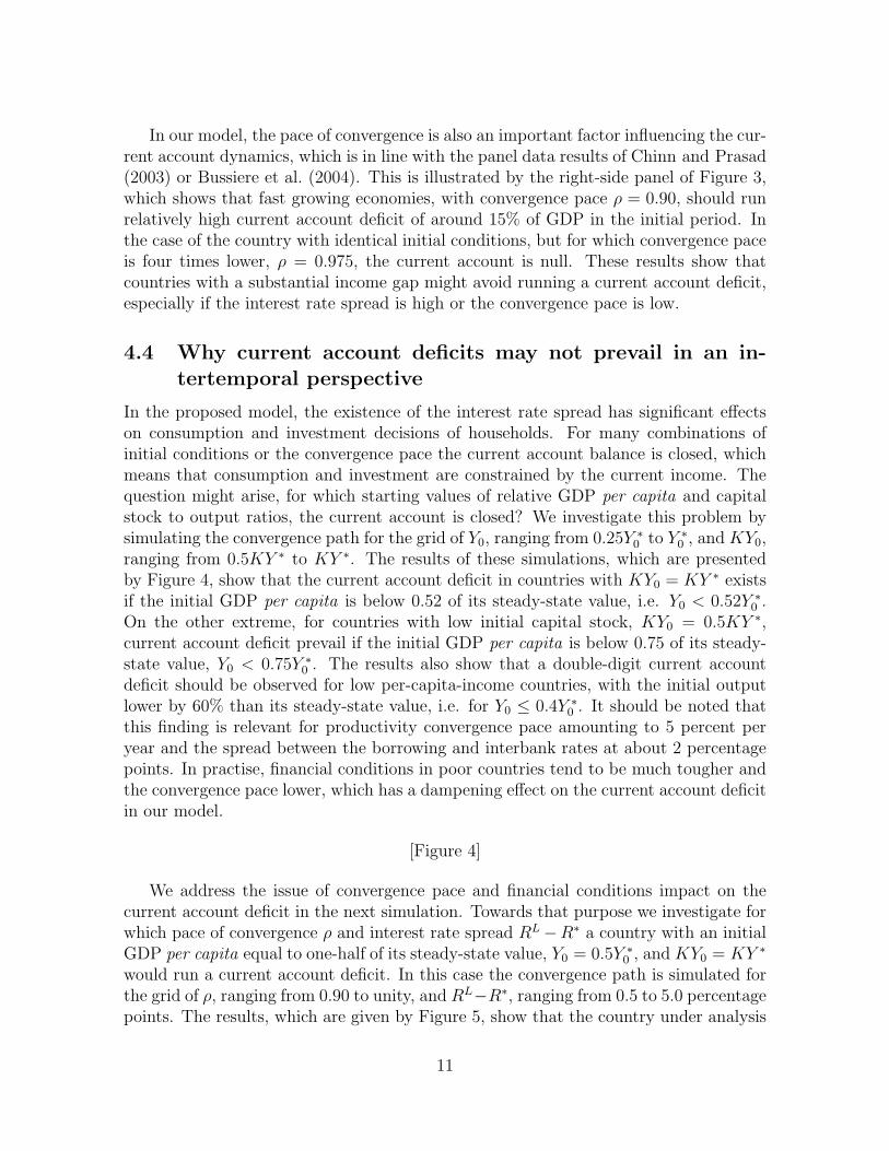
In our model, the pace of convergence is also an important factor influencing the cur-rent account dynamics, which is in line with the panel data results of Chinn and Prasad(2003) or Bussiere et al. (2004). This is illustrated by the right-side panel of Figure 3,which shows that fast growing economies, with convergence pace ρ = 0.90, should runrelatively high current account deficit of around 15% of GDP in the initial period. Inthe case of the country with identical initial conditions, but for which convergence paceis four times lower, ρ = 0.975, the current account is null. These results show thatcountries with a substantial income gap might avoid running a current account deficit,especially if the interest rate spread is high or the convergence pace is low.

4.4 Why current account deficits may not prevail in an in-tertemporal perspective

In the proposed model, the existence of the interest rate spread has significant effectson consumption and investment decisions of households. For many combinations ofinitial conditions or the convergence pace the current account balance is closed, whichmeans that consumption and investment are constrained by the current income. Thequestion might arise, for which starting values of relative GDP per capita and capitalstock to output ratios, the current account is closed? We investigate this problem bysimulating the convergence path for the grid of Y0, ranging from 0.25Y ∗

0 to Y ∗0 , and KY0,

ranging from 0.5KY ∗ to KY ∗. The results of these simulations, which are presentedby Figure 4, show that the current account deficit in countries with KY0 = KY ∗ existsif the initial GDP per capita is below 0.52 of its steady-state value, i.e. Y0 < 0.52Y ∗

0 .On the other extreme, for countries with low initial capital stock, KY0 = 0.5KY ∗,current account deficit prevail if the initial GDP per capita is below 0.75 of its steady-state value, Y0 < 0.75Y ∗

0 . The results also show that a double-digit current accountdeficit should be observed for low per-capita-income countries, with the initial outputlower by 60% than its steady-state value, i.e. for Y0 ≤ 0.4Y ∗

0 . It should be noted thatthis finding is relevant for productivity convergence pace amounting to 5 percent peryear and the spread between the borrowing and interbank rates at about 2 percentagepoints. In practise, financial conditions in poor countries tend to be much tougher andthe convergence pace lower, which has a dampening effect on the current account deficitin our model.

[Figure 4]

We address the issue of convergence pace and financial conditions impact on thecurrent account deficit in the next simulation. Towards that purpose we investigate forwhich pace of convergence ρ and interest rate spread RL−R∗ a country with an initialGDP per capita equal to one-half of its steady-state value, Y0 = 0.5Y ∗

0 , and KY0 = KY ∗

would run a current account deficit. In this case the convergence path is simulated forthe grid of ρ, ranging from 0.90 to unity, and RL−R∗, ranging from 0.5 to 5.0 percentagepoints. The results, which are given by Figure 5, show that the country under analysis

11

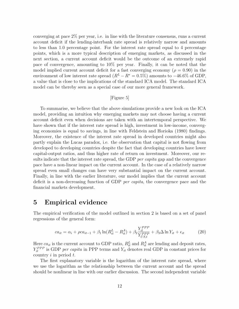
converging at pace 2% per year, i.e. in line with the literature consensus, runs a currentaccount deficit if the lending-interbank rate spread is relatively narrow and amountsto less than 1.0 percentage point. For the interest rate spread equal to 4 percentagepoints, which is a more typical description of emerging markets, as discussed in thenext section, a current account deficit would be the outcome of an extremely rapidpace of convergence, amounting to 10% per year. Finally, it can be noted that themodel implied current account deficit for a fast converging economy (ρ = 0.90) in theenvironment of low interest rate spread (RL−R∗ = 0.5%) amounts to −46.6% of GDP,a value that is close to the implications of the standard ICA model. The standard ICAmodel can be thereby seen as a special case of our more general framework.

[Figure 5]

To summarise, we believe that the above simulations provide a new look on the ICAmodel, providing an intuition why emerging markets may not choose having a currentaccount deficit even when decisions are taken with an intertemporal perspective. Wehave shown that if the interest rate spread is high, investment in low-income, converg-ing economies is equal to savings, in line with Feldstein and Horioka (1980) findings.Moreover, the existence of the interest rate spread in developed countries might alsopartly explain the Lucas paradox, i.e. the observation that capital is not flowing fromdeveloped to developing countries despite the fact that developing countries have lowercapital-output ratios, and thus higher rate of return on investment. Moreover, our re-sults indicate that the interest rate spread, the GDP per capita gap and the convergencepace have a non-linear impact on the current account. In the case of a relatively narrowspread even small changes can have very substantial impact on the current account.Finally, in line with the earlier literature, our model implies that the current accountdeficit is a non-decreasing function of GDP per capita, the convergence pace and thefinancial markets development.

5 Empirical evidence

The empirical verification of the model outlined in section 2 is based on a set of panelregressions of the general form:

cait = αi + ρcait−1 + β1 ln(RLit −RA

it) + β2Y PPP

it

Y PPPUS,t

+ β3∆ ln Yit + εit (20)

Here cait is the current account to GDP ratio, RLit and RA

it are lending and deposit rates,Y PPP

it is GDP per capita in PPP terms and Yit denotes real GDP in constant prices forcountry i in period t.

The first explanatory variable is the logarithm of the interest rate spread, wherewe use the logarithm as the relationship between the current account and the spreadshould be nonlinear in line with our earlier discussion. The second independent variable

12

is a proxy for the initial value of output, where GDP per capita in the US serves as areference value. The third explanatory is GDP growth rate, which as in Bussiere et al.(2004) is a proxy for the pace of convergence. We also added lagged dependent variableto account for current account persistence (see Chinn and Wei, 2008 for evidence).Finally, we assume that the error term consists of a country fixed effect αi and a residualerror εit, where fixed effects account for country specific factors such as demographicstructure, terms of trade volatility, openness and other factors which might be relevantfor the current account (see Faruqee and Debelle, 1996 or Chinn and Prasad, 2003 foran extended discussion).4

Our main interest is in the relationship between the current account and the interestrate spread. In line with our earlier considerations we expect that an increase in thespread should limit consumption smoothing and capital accumulation and thereby leadto a lower current account deficit. As a result we expect the sign of parameter β1

to be positive. As regards parameter β2 our prior is that it should be positive orinsignificant. If the interest rate spread is low or convergence pace fast, higher GDPper capita should increase the saving-investment balance. However, if financial marketsconditions or growth expectations are not favourable, then our model implies that thecurrent account is null and its level does not depend on the level of GDP per capita.Finally, for parameter β3 we expect a negative sign, so that the current account balancein the periods of fast convergence is lower, or that the parameter is insignificant.

The regression (20) is estimated in four versions, depending on the inclusion of lagged

dependent variable cait−1 and the last two independent variablesY PPP

it

Y PPPUS,t

and ∆ ln Yit. In

the case of specifications with restriction ρ = 0 we apply the two-stage least squareinstrumental variable estimator (IV), which controls for endogeneity, whereas for spec-ifications without the restriction parameters are estimated using the GMM estima-tor proposed by Arellano and Bover (1995) and fully developed in Blundell and Bond(1998).

The models are estimated using annual data from the period 1980-2006 for a largenumber of developing countries. To be comparable with the earlier panel-data liter-ature, we choose the sample of developing countries considered by Chinn and Prasad(2003), which we extend by central and eastern European countries that have joinedthe European Union in May 2004 and January 2007 (see Appendix for the detaileddescription of the dataset). The number of countries in the sample was constrainedby two limitations. First, the data for the deposit and lending rates are not availablefor all countries of our initial choice. Second, we remove observations for high interestrate periods, which we define as periods in which the lending rate stood above 25% andcould be viewed as periods of extreme instability, thus constituting clear outliers. As aresult the final sample includes sixty developing countries.

[Table 1]

4We are not using random effects since formal tests with the null that country specific randomeffects are uncorrelated with the regressors were rejected by the data.

13

The results, which are reported in Table 1, confirm the main hypothesis of ourtheoretical model: the interest rate spread has positive and significant impact on thecurrent account. The estimates show that doubling of the spread improves currentaccount balance by around 3% of GDP. This result is generally robust with respectto model specification and estimation. As regards estimates for relative output pa-rameter β2, they are not significantly different from zero and in dynamic specificationthe estimate has the wrong sign, which is broadly in line with the estimates for devel-oping countries of Chinn and Prasad (2003). We interpret this as partial support ofour model, which indicates that if the interest rate spread is high there should be norelationship between the current account and relative output (see Figure 5). The esti-mates of output growth parameter β3 are of expected sign and in the case of dynamicspecification the coefficient is significantly different from zero. Finally, we find sub-stantial persistence in the current account, where the estimate of ρ at 0.6 correspondsto estimates by Bussiere et al. (2004), who interpret this in terms of habit formationin the behaviour of households. Overall, we believe that the above results constitutesome evidence in favour of the proposed model, showing in particular the importance ofincluding the lending-borrowing spread to gauge the dynamics of the current account.

6 Conclusions

The standard intertemporal model of the current account assumes that the rates ondeposits and loans are the same. One of the implications of this assumption is thatfast-converging economies with initially low per capita output should run substantialcurrent account deficits, which are however hardly observed in practise. Moreover, inempirical applications the standard ICA model is often rejected by the data if present-value tests are used or forecast accuracy comparison is performed (see Bergin, 2003 and2006). In this paper we have argued that the poor performance of the standard ICAmodel might be to some degree explained by the existence of the lending-deposit interestrate spread. For that purpose we have developed a perfect-foresight general equilibriummodel with two interest rates. Then we have performed a series of simulations toshow that even a small change in the interest rate spread might have a tremendouseffect on the current account balance, especially if the interest rate spread is close tozero. Moreover, we have indicated that the existence of the interest rate spread mightprevent developing countries from running current account deficits, even in the case ofeconomies experiencing rapid productivity growth. Finally, on the basis of the paneldata for a large number of developing countries we have shown that the implications ofthe proposed model are to some degree confirmed by the data.

Further research related to the proposed framework can evolve in many directions.First, the specification of the model could be developed to embody other features thatmay be appropriate in explaining current account fluctuations. One could relax the one-good assumption and suppose an infinite number of goods sold at the monopolisticallycompetitive market. This would have a dampening effect on the model’s predictions for

14

the current account deficits in converging economies as the future repayment of foreignliabilities would require a deterioration in the terms of trade (Blanchard and Giavazzi,2002). The model could also be developed to include traded and non-traded goodsto address the relative price implications of the convergence process, as it is done byFagan and Gaspar (2007). Second, the proposed framework could be extended into astochastic setup to analyse the implications of the lending-deposit interest rate spreadon the shape of response of the current account to structural shocks, temporary produc-tivity shock for instance. Finally, it might be interesting to introduce the two-interestrate setup to models other than those aimed at analysing current account developments.For instance, it might be interesting to see whether the existence of the interest ratespread has an effect on the response of the economy to a monetary shock. It shouldbe noted that recently few authors proposed closed economy DSGE models with twointerest rates (e.g. Gerali et al., 2009, or Curdia and Woodford, 2009). The proposedsolutions, however, are based on very strong assumptions, which are introduced in away that enables to use standard perturbation techniques of solving DSGE models:Gerali et al. (2009) assume a very specific form of heterogeneity in time preferencesand (Curdia and Woodford, 2009) in the utility function.

To summarise, it is evident that the role of two interest rates is relatively unex-plored field in microfunded optimising models, which dominate currently in the modernmacroeconomics. These models assume that rates on deposits and loans are the same,which is strongly in opposition to what we observe in reality. In this paper we haveshown that the existence of the interest rate spread can change significantly the impli-cations of the standard ICA model for the current account dynamics. We put forward ahypothesis that the existence of the spread has an important impact on the dynamics ofother macroeconomic variables, the verification of which we leave for further research.

Appendix

The data used in section 5 are taken from the World Economic Outlook 2009 (WEO)released by the International Monetary Fund, as well as the World Development Indica-tors (WDI) database of the World Bank. The relevant tickers for raw data are as follows:the current account to GDP ratio (WEO, bca ngdpd), GDP per capita in PPP terms(WEO, ppppc), annual percent change of constant price GDP (WEO, ngdp rpch), thelending rate (WDI, m4413244409) and the deposit rate (WDI, m1413519881).

Countries included are as follows: Algeria, Argentina, Bangladesh, Benin, Botswana,Bulgaria, Burkina Faso, Burundi, Cameroon, Chile, Colombia, Congo, Costa Rica, CoteD’Ivoire, Dominica, Ecuador, Egypt, El Salvador, Estonia, Gabon, Ghana, Gambia,Guatemala, Honduras, Hungary, Indonesia, Jamaica, Jordan, Kenya, Latvia, Lithuania,Malaysia, Malawi, Mali, Mauritius, Mexico, Morocco, Nepal, Niger, Nigeria, Panama,Papua New Guinea, Peru, Philippines, Poland, Rwanda, Senegal, Seychelles, SierraLeone, South Africa, Sri Lanka, Swaziland, Syria, Thailand, Togo, Trinidad & Tobago,Uganda, Venezuela, Zambia, Zimbabwe.

15

References

Arellano, Manuel, and Bover, Olympia. 1995. Another look at the instrumental variableestimation of error-components models. Journal of Econometrics, 68(1), 29–51.

Benigno, Pierpaolo. 2009. Price Stability with Imperfect Financial Integration. Journalof Money, Credit and Banking, 41(s1), 121–149.

Bergin, Paul R. 2003. Putting the ’New Open Economy Macroeconomics’ to a test.Journal of International Economics, 60(1), 3–34.

Bergin, Paul R. 2006. How well can the New Open Economy Macroeconomics explainthe exchange rate and current account? Journal of International Money and Finance,25(5), 675–701.

Bergin, Paul R, and Sheffrin, Steven M. 2000. Interest rates, exchange rates and presentvalue models of the current account. Economic Journal, 110(463), 535–58.

Blanchard, Olivier, and Giavazzi, Francesco. 2002. Current account deficits in the euroarea: The end of the Feldstein Horioka puzzle? Brookings Papers on EconomicActivity, 33(2), 147–210.

Blundell, Richard, and Bond, Stephen. 1998. Initial conditions and moment restrictionsin dynamic panel data models. Journal of Econometrics, 87(1), 115–143.

Buiter, Willem H. 1981. Time preference and international lending and borrowing inan overlapping-generations model. Journal of Political Economy, 89(4), 769–97.

Bussiere, Matthieu, Fratzscher, Marcel, and Muller, Gernot J. 2004. Current accountdynamics in OECD and EU acceding countries - an intertemporal approach. WorkingPaper Series 311. European Central Bank.

Ca’ Zorzi, Michele, and Rubaszek, Michal. 2008. On the empirical evidence of theintertemporal current account model for the euro area countries. Working PaperSeries 895. European Central Bank.

Campbell, John Y. 1987. Does saving anticipate declining labor income? An alternativetest of the Permanent Income Hypothesis. Econometrica, 55(6), 1249–73.

Chinn, Menzie D., and Prasad, Eswar S. 2003. Medium-term determinants of currentaccounts in industrial and developing countries: An empirical exploration. Journalof International Economics, 59(1), 47–76.

Chinn, Menzie D., and Wei, Shang-Jin. 2008. A Faith-based Initiative: Does a Flex-ible Exchange Rate Regime Really Facilitate Current Account Adjustment? NBERWorking Papers 14420. National Bureau of Economic Research, Inc.

16

Curdia, Vasco, and Woodford, Michael. 2009. Credit Spreads and Monetary Policy.NBER Working Papers 15289. National Bureau of Economic Research, Inc.

Fagan, Gabriel, and Gaspar, Vıtor. 2007. Adjusting to the euro. Working Paper Series716. European Central Bank.

Faruqee, Hamid, and Debelle, Guy. 1996. What determines the current account? Across-sectional and panel approach. IMF Working Papers 96/58. International Mon-etary Fund.

Feldstein, Martin, and Horioka, Charles. 1980. Domestic Saving and InternationalCapital Flows. Economic Journal, 90(358), 314–29.

Fisher, Irving. 1930. The Theory of Interest. New York: Macmillan.

Galı, Jordi, Lopez-Salido, J. David, and Valles, Javier. 2007. Understanding the ef-fects of government spending on consumption. Journal of the European EconomicAssociation, 5(1), 227–270.

Gerali, Andrea, Neri, Stefano, Sessa, Luca, and Signoretti, Federico M. 2009. Creditand banking in a DSGE model of the euro area. mimeo, Bank of Italy.

Gruber, Joseph W. 2004. A present value test of habits and the current account. Journalof Monetary Economics, 51(7), 1495–1507.

Hassin, Rafael, and Lieber, Zvi. 1982. Optimal consumption with a stochastic incomestream and two interest rates. Southern Economic Journal, 49, 482–493.

Hayashi, Fumio. 1982. Tobin’s marginal q and average q: A neoclassical interpretation.Econometrica, 50(1), 213–24.

Lane, Philip R., and Milesi-Ferretti, Gian Maria. 2001. The external wealth of nations:Measures of foreign assets and liabilities for industrial and developing countries. Jour-nal of International Economics, 55(2), 263–294.

Nason, James M., and Rogers, John H. 2006. The present-value model of the currentaccount has been rejected: Round up the usual suspects. Journal of InternationalEconomics, 68(1), 159–187.

Nehru, Vikram, and Dhareshwar, Ashok. 1993. A New Database on Physical CapitalStock: Sources, Methodology and Results. Revista de Analisis Economica, 8(1),37–59.

Obstfeld, Maurice, and Rogoff, Kenneth. 1996. The intertemporal approach to the cur-rent account. NBER Working Papers 4893. National Bureau of Economic Research,Inc.

17

Otto, Glenn. 1992. Testing a present-value model of the current account: Evidencefrom US and Canadian time series. Journal of International Money and Finance,11(5), 414–430.

Roeger, Werner, and in ’t Veld, Jan. 2004. Some selected simulation experiments withthe European Commission’s QUEST model. Economic Modelling, 21(5), 785–832.

Sachs, Jeffrey D. 1981. The current account and macroeconomic adjustment in the1970s. Brookings Papers on Economic Activity, 12(1), 201–282.

Schmitt-Grohe, Stephanie, and Uribe, Martin. 2003. Closing small open economy mod-els. Journal of International Economics, 61(1), 163–185.

Sheffrin, Steven M., and Woo, Wing Thye. 1990. Present value tests of an intertemporalmodel of the current account. Journal of International Economics, 29(3-4), 237–253.

Singh, Tarlok. 2007. Intertemporal optimizing models of trade and current accountbalance: A survey. Journal of Economic Surveys, 21(1), 25–64.

Watkins, Thayer H. 1969. Borrowing-lending interest rate differentials and the timeallocation of consumption. Cowles Foundation Discussion Papers 282. Cowles Foun-dation, Yale University.

Zorzi, Michele Ca’, Chudik, Alexander, and Dieppe, Alistair. 2009 (Jan.). Currentaccount benchmarks for central and eastern Europe - a desperate search? WorkingPaper Series 995. European Central Bank.

18

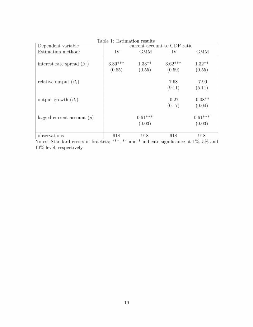
Table 1: Estimation resultsDependent variable current account to GDP ratioEstimation method: IV GMM IV GMM

interest rate spread (β1) 3.30*** 1.33** 3.62*** 1.32**(0.55) (0.55) (0.59) (0.55)

relative output (β2) 7.68 -7.90(9.11) (5.11)

output growth (β3) -0.27 -0.08**(0.17) (0.04)

lagged current account (ρ) 0.61*** 0.61***(0.03) (0.03)

observations 918 918 918 918Notes: Standard errors in brackets; ***, ** and * indicate significance at 1%, 5% and10% level, respectively

19

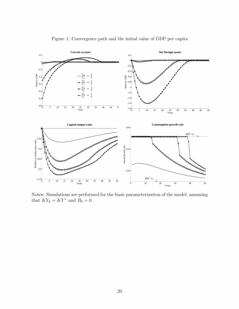
Figure 1: Convergence path and the initial value of GDP per capita

0 5 10 15 20 25 30 35 40 45 50-0.6

-0.5

-0.4

-0.3

-0.2

-0.1

0

0.1Current account

Rat

io to

GD

P

Years

Y0

Y∗

0

=3

4

Y0

Y∗

0

=1

2

Y0

Y∗

0

=1

3

Y0

Y∗

0

=1

4

0 5 10 15 20 25 30 35 40 45 50-1.8

-1.6

-1.4

-1.2

-1

-0.8

-0.6

-0.4

-0.2

0

0.2Net foreign assets

Rat

io to

GD

P

Years

0 5 10 15 20 25 30 35 40 45 500.75

0.8

0.85

0.9

0.95

1

Capital-output ratio

Rel

ativ

e to

ste

ady-

stat

e va

lue

Years 0 10 20 30 40 50

0.02

0.03

0.04Consumption growth rate

Ann

ual g

row

th r

ate

Years

β(RL-1)

β(R*-1)

Notes: Simulations are performed for the basic parameterization of the model, assumingthat KY0 = KY ∗ and B0 = 0.

20

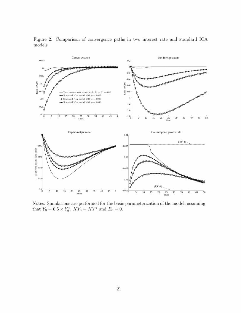
Figure 2: Comparison of convergence paths in two interest rate and standard ICAmodels

0 5 10 15 20 25 30 35 40 45 50-0.3

-0.25

-0.2

-0.15

-0.1

-0.05

0

0.05Current account

Rat

io to

GD

P

Years

Two interest rate model with RL −R∗ = 0.02

Standard ICA model with φ = 0.005

Standard ICA model with φ = 0.020

Standard ICA model with φ = 0.040

0 5 10 15 20 25 30 35 40 45 50-1.6

-1.4

-1.2

-1

-0.8

-0.6

-0.4

-0.2

0

0.2Net foreign assets

Rat

io to

GD

P

Years

0 5 10 15 20 25 30 35 40 45 500.8

0.84

0.88

0.92

0.96

1Capital-output ratio

Rel

ativ

e to

ste

ady-

stat

e va

lue

Years 0 5 10 15 20 25 30 35 40 45 500.015

0.02

0.025

0.03

0.035

0.04Consumption growth rate

Years

β(R*-1)

β(RL-1)

Notes: Simulations are performed for the basic parameterization of the model, assumingthat Y0 = 0.5× Y ∗

0 , KY0 = KY ∗ and B0 = 0.

21

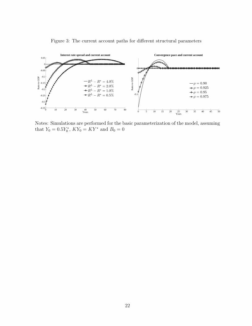
Figure 3: The current account paths for different structural parameters

0 10 20 30 40 50 60 70 80-0.35

-0.3

-0.25

-0.2

-0.15

-0.1

-0.05

0

0.05Interest rate spread and current account

Rat

io to

GD

P

Years

RL−R

∗ = 4.0%

RL−R

∗ = 2.0%

RL−R

∗ = 1.0%

RL−R

∗ = 0.5%

0 5 10 15 20 25 30 35 40 45 50

-0.1

0

Convergence pace and current account

Rat

io to

GD

P

Years

ρ = 0.90

ρ = 0.925

ρ = 0.95

ρ = 0.975

Notes: Simulations are performed for the basic parameterization of the model, assumingthat Y0 = 0.5Y ∗

0 , KY0 = KY ∗ and B0 = 0

22

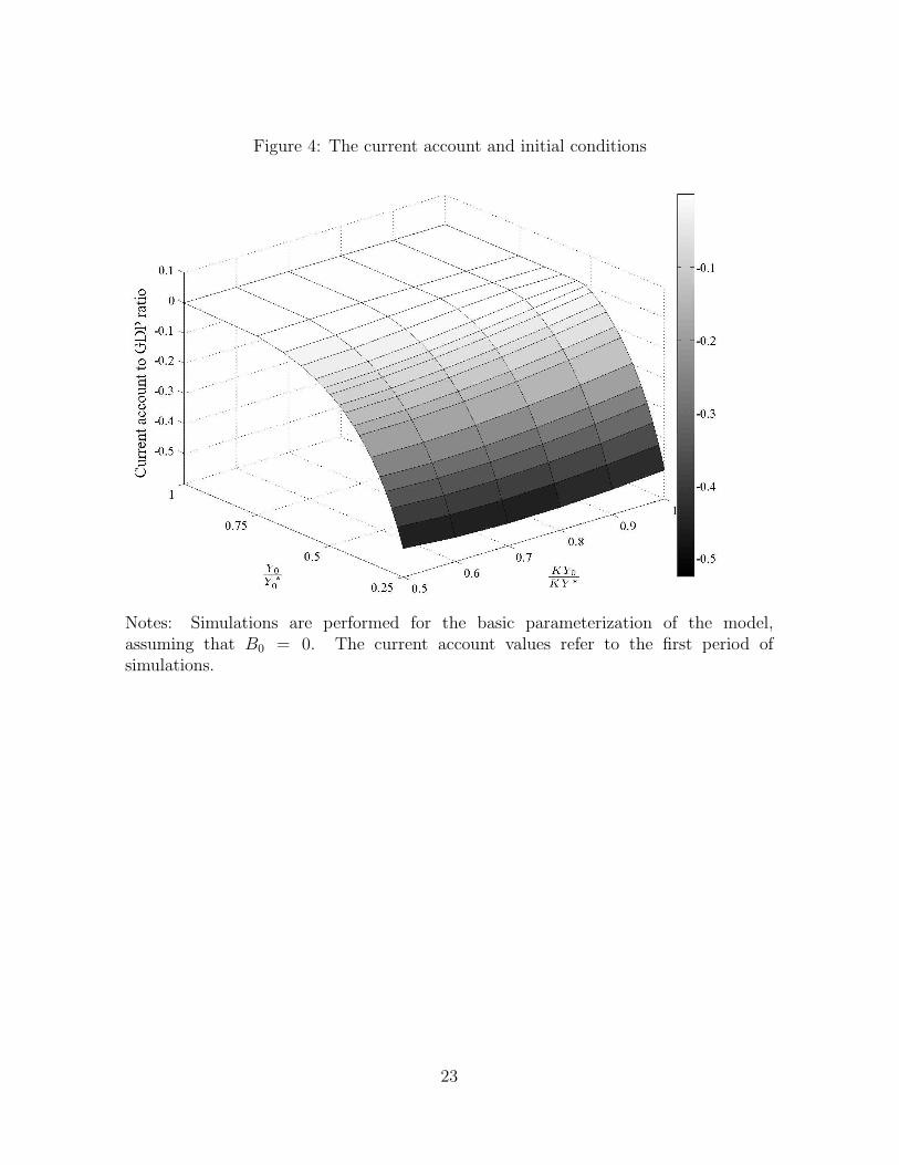
Figure 4: The current account and initial conditions

Notes: Simulations are performed for the basic parameterization of the model,assuming that B0 = 0. The current account values refer to the first period ofsimulations.

23

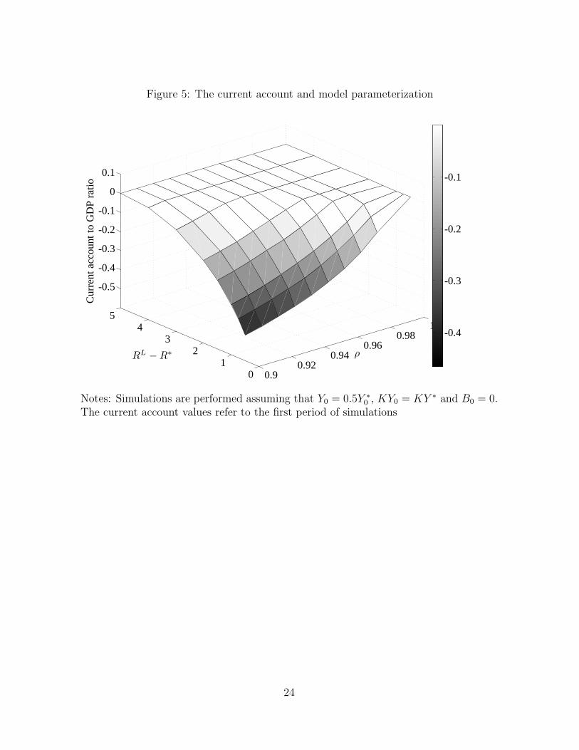
Figure 5: The current account and model parameterization

01

23

45

0.90.92

0.940.96

0.981

-0.5

-0.4

-0.3

-0.2

-0.1

0

0.1

ρRL −R∗

Cur

rent

acc

ount

to G

DP

ratio

-0.4

-0.3

-0.2

-0.1

Notes: Simulations are performed assuming that Y0 = 0.5Y ∗0 , KY0 = KY ∗ and B0 = 0.

The current account values refer to the first period of simulations

24