Embed Size (px)
Citation preview

Hurricanes:
Intertemporal Trade and Capital Shocks
John C. Bluedorn†
Dept. of Economics, University of OxfordManor Road Building, Manor Road
Oxford OX1 3UQUnited Kingdom
Email: [email protected].: +44 (0) 1865-281-483Fax: +44 (0) 1865-271-094
May 2005
Abstract: Hurricanes in the Caribbean and Central America represent a natural ex-periment to test the intertemporal approach to current account determination. Theintertemporal approach allows for the possibility of intertemporal trade, via interna-tional borrowing. Previous tests of intertemporal current account (ICA) models havetypically relied upon the identification of shocks in a VAR framework with which to tracethe current account response. Hurricane shocks represent exactly the kind of temporary,country-specific shock required by the theory, allowing for the intertemporal current ac-count response to be estimated without recourse to a VAR shock decomposition. Usingdata on the economic damages attributable to a hurricane, I estimate the economy’sresponse to a hurricane-induced capital shock within a fixed effects panel model. Thecurrent account response qualitatively conforms to the S-shaped response predicted bythe theory, indicating that countries are engaging in intertemporal trade. However, theexact timing and magnitude of the response differs from a standard ICA model’s smoothbehavior. A hurricane which destroys capital valued at one year’s GDP pushes the cur-rent account over GDP into deficit by 5 percentage points initially. 3-8 years after sucha hurricane, the current account over GDP moves into surplus at 2.7 percentage points.
JEL Classification: F320, F410Keywords: hurricanes, natural experiment, current account dynamics
†This paper is a greatly revised version of the first chapter of my dissertation. Special thanks toDavid Romer, Maurice Obstfeld, Andrew Rose, and Michael Jansson for their guidance and comments.I would also like to thank Bjorn Brugemann, Elizabeth Cascio, Paola Guiliano, Rebecca Hellerstein, andHui Tong for their feedback. All errors are mine.

1 Introduction
In the 1970s, the OPEC oil price shocks generated large current account imbalances.
Oil-consuming countries borrowed extensively on the international capital market to pay
higher oil prices, while oil-producing nations sought out investment opportunities for their
revenue windfall. Traditional Keynesian models did not provide much insight into the
long-run consequences of such shocks for external debt sustainability, as they failed to
account for the intertemporal budget constraint. Around the same time, Lucas (1976)
argued that reliable macroeconomic policy analysis needed a firm grounding in theoretical
models explicitly based on economic agents’ forward-looking behavior. The intertemporal
approach to the current account emerged in the early 1980s as an attempt to understand
the consequences of external shocks for an open economy within a forward-looking dy-
namic optimization framework.1 Following models such as the Ramsey-Cass-Koopmans
and Diamond models, an intertemporal current account (ICA) model describes the open
macroeconomy’s dynamics as the solution to a representative agent’s optimization prob-
lem, subject to an intertemporal budget constraint. Its fundamental innovation is the
introduction of forward-looking intertemporal trade which occurs through international
borrowing. Intertemporal trade allows the agent to save and borrow in response to
country-specific shocks in order to smooth the evolution of the marginal utility of con-
sumption, while maximizing returns.2 An ICA model thus predicts a specific empiri-
cal relationship between movements in a country’s current account and country-specific
shocks.
Although presenting an intuitive framework to understand current account dynamics,
most empirical tests have rejected the intertemporal approach to the current account. I
1For a good account of the basic history and origins of the intertemporal approach, see Obstfeld andRogoff [1995] and Obstfeld and Rogoff [1996]. Intellectually, the intertemporal approach is a precursorin the development of the New Open Economy Macroeconomics. New Open Economy models enhancea standard intertemporal current account model by introducing imperfect competition and nominalrigidities [Lane, 2001].
2 When everyone is subject to the same shock, there is no differential across countries to makerisk-sharing through borrowing and lending desirable. Formally, the world real interest rate changes toeliminate the gains from borrowing and lending in response to a global shock. Thus, the current accountdoes not generally respond to global shocks.
1

suggest that many of the documented empirical rejections of ICA models may be due to
violations of the auxiliary assumptions required in structural tests (detailed later) and
the failure to properly identify country-specific shocks.
I argue that hurricanes represent a natural experiment in which to test the predictions
of an ICA model. Hurricanes are large, temporary, exogenous, negative country-specific
capital shocks. In this paper, I evaluate the responses of the small, open economies of the
Caribbean and Central America to large hurricane shocks. Some of these economies are
exceptionally small. For example, St. Kitts and Nevis and Antigua and Barbuda both
have populations under a hundred thousand. In the markets in which they participate,
they clearly take world economic conditions as given. They do not influence world prices
or interest rates. Such economies are real world counterparts to the theoretical construct
of small, open economies.
Using economic damages attributable to a storm, I find evidence that countries do
engage in intertemporal trade in response to hurricane shocks, thus broadly supporting
the key prediction of an ICA model. In response to an unanticipated, negative capital
shock, an ICA model predicts that the country experiences an immediate fall in output.
Accompanying the fall in output is a fall in saving (from consumption smoothing) and a
rise in investment (to replace the capital destroyed). In sum, these responses imply a fall
in the current account, identical to a fall in net foreign assets or a rise in international
borrowing. After the initial shock, output is predicted to recover and investment to fall
back to its steady state level. The exact predicted future current account and saving
responses depend on the relationship between a country’s rate of time preference and the
world interest rate, as this determines how the intertemporal budget constraint binds.
For a relatively impatient country, both saving and the current account are predicted to
rise in the future. If the country is relatively patient, then saving and the current account
remain below what they would have been in the absence of the capital shock.3 Deaton
3An economy’s degree of patience is related to its long-run propensity to be a debtor (impatient) ora creditor (patient). Notice how this is potentially related to Kraay and Ventura’s [2000] observationthat debtor and creditor economies may exhibit different current account responses.
2
[1990] argued that impatience is the more realistic assumption in modelling developing
countries. I follow him by focusing on the impatient case. When capital adjustment costs
are introduced into the model, the responses of all the variables are slowed. Furthermore,
the response magnitudes are reduced, as adjustments are spread over a greater period of
time.
Corresponding to the primary variables of the standard ICA model, I investigate the
effect of a hurricane shock on: the current account over GDP, the national saving rate,
capital investment rate, real per capita output growth, and real per capita consumption
growth. I also consider the effect of a hurricane shock on a set of additional variables
which may be significant drivers of current account behavior in light of a large capital
shock, but about which the standard ICA model is silent. These include: net transfers
from abroad over GDP, foreign aid over GDP, worker remittances over GDP, and the
government budget deficit over GDP.
I estimate a heteroskedasticity and autocorrelation robust panel model for each of
the macroeconomic variable’s listed above, including both country and time fixed effects.
The country fixed effect captures the country-specific trend in a macroeconomic vari-
able, while the time fixed effect captures any global shocks experienced by the region.
Hurricane economic damages and its lags are the explanatory variables in the baseline
regression. I then allow for different responses across countries by introducing various
country-specific characteristics interacted with the damages measure. The coefficients on
hurricane economic damages, its lags and interactions thus embody the reduced form im-
pulse response of the macroeconomic variable to a hurricane shock, allowing the response
to be unrestricted.
The empirical results support an ICA model’s qualitative predictions. There is clear
evidence of intertemporal trade taking place in response to the large, country-specific,
negative capital shocks caused by hurricanes. This manifests as a current account re-
sponse that is similar to that described above: the current account falls initially, as
output falls and investment rises; the current account then rises, as saving rises and in-
3

vestment falls. The results indicate a 5 percentage point decline in the current account
to GDP ratio in the year after a large hurricane shock.4 3-8 years after a hurricane
shock, the current account to GDP ratio rises approximately 2.7 percentage points above
its long-run trend. Such an S-shaped intertemporal response is consistent with an ICA
model, but not with an atemporal model. However, the estimated current account re-
sponse’s timing and magnitude differs from the predictions of a standard ICA model.
This suggests several modifications to a standard ICA model, all of which influence the
rate at which the intertemporal budget constraint binds.
The paper proceeds as follows. In Section 2, I discuss the empirical record of ICA
models, examining how previous tests might generate false rejections. In Section 3,
I present more information regarding hurricanes as a natural experiment, generating
random changes in the size of a country’s physical capital stock. In Section 4, I present
a standard ICA model and discuss its predictions. In Section 5, I describe the hurricane
economic damages’ measure and the macroeconomic data used in the analysis. In Section
6, I discuss the panel data model I employ to estimate the macroeconomic response to a
hurricane. In Section 7, the empirical results of the analysis are presented. In Section 8, I
discuss the economic significance of the findings and their implications for intertemporal
models. In Section 9, I conclude by summarizing and interpreting my findings more
broadly.
2 The Empirical Record of Intertemporal Current
Account Models
Two broad approaches have developed to test ICA models. They employ different strate-
gies to achieve the identification of shocks and thus ensure proper statistical inference on
the current account response.
4A large hurricane shock is one which inflicts capital stock damages equal to a year’s GDP. Thechanges in the current account to GDP ratio are relative to trend.
4

The first research approach is structural. Inspired by Campbell’s 1987 innovation in
testing present-value models, the structural approach exploits the information structure
implied by a forward-looking rational expectations model to establish identification.5
Under certain assumptions, an ICA model implies a simple formulation of the current
account, as the negative expectation of the present-value of net output. The identification
assumption effectively allows for the current account response to shocks to be recovered in
a VAR framework. Applications of present-value tests to an ICA model include Sheffrin
and Woo [1990], Otto [1992], Ghosh [1995], and Ghosh and Ostry [1995].
The second research approach is nonstructural. Political and natural events that are
plausibly exogenous are used to achieve the identification of temporary country-specific
shocks, which can then be directly used to estimate the current account response. Ahmed
[1987] follows such an approach. Arguing that wars are exogenous and temporary, he
examines the relationship between public military spending (government budget deficits)
and the trade balance in the United Kingdom from 1723 to 1913.6 He then compares
the observed responses of economic variables to the predictions of an ICA model. The
“natural experiment” afforded by wartime public spending thus generates identification
in the analysis.
Each approach presents its own advantages and disadvantages for proper inference.
There are three main drawbacks to empirical testing of ICA models using structural
present-value tests. First, a rejection of the model could be due to any one of the
auxiliary assumptions required for the formulation of the present-value test. These
include: (1) quadratic period utility; (2) a rate of time preference that is equal to the
world real interest rate; and (3) shocks that follow a martingale difference process.7 The
model is thus an open economy version of the permanent income (PI) model. Second,
5Specifically, an unobserved components structure is assumed for choice variables. The unobservedcomponents capture information available to the agent, but not to the econometrician. Observed choicesby agents under rational expectations then become sufficient statistics for the unobserved components(or shocks). This allows for the expectation of future net output flows to be evaluated, which determinesthe current account under the null.
6Ahmed [1986] used a similar approach to investigate crowding out and Ricardian equivalence.7The last assumption means that conditional expectations are linear projections on past information,
yielding a standard VAR prediction framework.
5

a present-value test fails to differentiate between global and country-specific shocks. An
ICA model predicts a current account response to country-specific shocks, whereas global
shocks (which affect all countries) result in no current account response.8 Glick and
Rogoff [1995] demonstrated the importance of the global versus local shock distinction in
their study of the effect of productivity shocks on the current account and investment.
Present-value tests implicitly treat all shocks as country-specific, potentially leading to
over-rejection of the ICA model. Third, even if all shocks are in fact country-specific,
Kasa [2003] demonstrates that present-value tests are not necessarily revelatory about the
underlying shocks. Temporary (or transitory) and permanent shocks will generally have
different effects, and thus distinguishing between these two types of shocks when testing
is important. Considering an ICA PI model with additive net output shocks, Kasa
demonstrates that Campbell’s method will lead to erroneous inference in certain regions
of the parameter space. When the moving average representation with respect to the
true shocks is non-invertible, Campbell’s method will extract “transitory” shocks that are
in fact a combination of the true transitory and permanent shocks. When the measured
current account response does not react fully to the “transitory” shock, a present-value
test will tend to reject the model.9 This can occur for a variety of reasonable parameter
values. Taken together, these caveats cast doubt on the generally negative statistical
results found in most present-value tests of ICA models. In fact, Kasa remarks that
the focus on present-value tests of the ICA model has arguably lead to a “technological
regress” in the effective decomposition and identification of shocks, which is necessary for
empirical tests of ICA models.
The structural approach using present-value tests makes strong, unambiguous quanti-
tative predictions under the null. It implies that the parameters of the VAR must satisfy
certain restrictions.10 In contrast, testing under the non-structural approach does not
8See footnote 2.9The failure to adequately differentiate between transitory and permanent shocks could also result in
a false acceptance of the model.10See Obstfeld and Rogoff [1995, 1996] for a clear exposition of these restrictions.
6

typically make such clear quantitative predictions.11 If one is interested in measuring
quantitatively how closely an ICA model predicts the actual current account response,
the empirical response of the current account must be compared with the quantitative
predictions from a calibrated theoretical model. However, the qualitative predictions
of an intertemporal model of the current account differ from the qualitative predictions
of an atemporal model, such as the classic Mundell-Fleming model. The difference in
qualitative predictions between intertemporal and atemporal models arises from the lack
of an intertemporal budget constraint in an atemporal model. The intertemporal budget
constraint implies that the current account must exhibit long-run convergence. Thus, a
qualitative comparison of the predicted response with the actual response can distinguish
the intertemporal and atemporal models.12
There have been several attempts to rehabilitate present-value tests of ICA models,
by making various modifications to the canonical present-value ICA model (described
above). These include introducing time non-separable preferences (via habit formation
in consumption), country-specific fiscal policy shocks, world real interest rate shocks,
and imperfect international capital mobility (via an upward-sloping supply curve for
international debt). Nason and Rogers [2003] review this literature and present a model
which nests all of these modifications. Using an interesting Bayesian framework, they
test how closely the estimated response from synthetic data generated by the modified
ICA model matches the estimated response from actual data.13 They find that world
real interest rate shocks do the most to move the model predictions closest to the actual
response, perhaps highlighting the importance of the global versus country-specific shock
11A notable exception is related to the classic Feldstein-Horioka 1980 regression, which soundly rejectedthe intertemporal prediction that investment and saving are contemporaneously unrelated. However,the endogeneity of investment and saving means that a proper test of this prediction requires that awindfall change in income or wealth be used to instrument saving, as only such a windfall change wouldleave capital returns unchanged. Clearly, a physical capital shock, such as a hurricane, does not fulfillthis requirement, meaning that it cannot be used to instrument for saving.
12Of course, with sufficient ad hoc assumptions, an atemporal model can exactly replicate the currentaccount predictions of an intertemporal model, rendering the two models observationally equivalent.In an unpublished appendix (Appendix A.2), I present a standard atemporal model which generatespredictions different from those of an intertemporal model. It imposes a set of limited but plausibleassumptions.
13The estimated response from actual data is derived from the standard present-value test.
7

distinction. While attending to some of the concerns regarding the auxiliary theoretical
assumptions of present-value tests, these modifications to structural present-value tests
of the ICA still fail to truly distinguish between country-specific and global shocks, and
to identify temporary and permanent shocks.14
Employing the shock decompositions implied by various econometric models, other
work has improved shock identification. Exploiting the long-run budget constraint,
Corsetti and Konstantinou [2004] use a cointegration framework to quantify temporary
and permanent innovations to net output flows for the United States. Although unable
to distinguish between country-specific and global shocks, their findings are generally
supportive of an ICA model.15 Giannone and Lenza [2004] use a generalized dynamic
factor model to allow for country-specific responses to global shocks. With the resulting
identification of country-specific shocks, they show that the Feldstein-Horioka puzzle
vanishes after the 1970s, thus supporting an ICA model. However, it is difficult to
interpret what exactly the identified statistical global shocks are.
Recently, Gournichas and Rey [2005] have presented another explanation for empirical
rejections of ICA models, in particular for developed economies. By failing to consider the
portfolio composition of net foreign assets (the stock counterpart of the current account),
potentially important valuation effects are neglected.16 They present results for the
United States which support this interpretation, indicating that valuation effects may
aid the US in eventually achieving external balance.17 However, such valuation effects
are likely not as relevant for developing economies, as Obstfeld [2004] explains. A rough
14Kasa [2003] notes that identifying temporary and permanent additive net output shocks is feasiblein the framework of a present-value test, if one uses the moving-average representation of the processdirectly. Hansen and Sargent [1991] present other possible remedies.
15In related work, Hoffmann [2001, 2003] decomposes temporary and permanent, country-specific andglobal shocks in a VAR framework by employing various orthogonality assumptions.
16In related work emphasizing a portfolio-based interpretation of the current account, Kraay and Ven-tura [2000, 2003] show that if investment risk is high and diminishing returns to capital are weak, currentaccount behavior differs across debtor and creditor economies. In the presence of capital adjustmentcosts, the short-run behavior of the current account emphasizes movements in net foreign assets as ashock-absorber, while the long-run behavior of the current account reflects portfolio concerns. In regres-sions of the current account on portfolio-adjusted saving, they demonstrate that their model effectivelyaddresses the Feldstein-Horioka puzzle and thus supports an intertemporal model. However, as with allFeldstein-Horioka type regressions, endogeneity is an issue.
17Tille [2004] forcefully demonstrates the potential size of the valuation effect for the US.
8

decomposition of net foreign assets into development finance (intertemporal trade) and
diversification finance (intra-temporal portfolio asset trades) reveals that diversification
finance is significantly less operative in developing economies.
In the current paper, I revive the non-structural approach to testing an ICA model,
arguing that hurricanes are the temporary, country-specific shocks required by the theory.
With a natural experiment research design, it will not be necessary to infer the size or
quality of shocks via a VAR-type decomposition. The natural experiment generates the
appropriate shock identification.
3 Hurricanes as Natural Experiments
Each year, the Atlantic basin experiences an average of 9.8 named storms (storms with
maximum wind speeds of at least 18 meters per second).18 Figure 1 shows the quinten-
nial distribution of named storms since 1960. It includes information on their relative
strength. There is substantial interannual variation in storm activity [Landsea et al.,
1999]. Of storms affecting the Caribbean and Central America, only a few each year are
destructive enough to significantly impact a country’s macroeconomy. Pictures of the
size of such devastating storms can be seen in Figure 2. These storms can completely
engulf an unfortunate island country. The damage wrought by a storm can include home
and building destruction, severe beach erosion, and crop and agricultural capital destruc-
tion, such as banana trees (see Elsner and Kara [1999]). From an economic perspective,
a strong hurricane manifests primarily as a large negative capital shock.19
Do such hurricane shocks need to be completely unanticipated in order for a current
account effect to manifest, under a standard ICA model? An unanticipated shock causes
a deterioration of the current account in an ICA model, as the representative agent
attempts to smooth consumption and maximize returns to domestic capital by borrowing
18Hurricanes are the strongest of named storms.19Although there can be terrible human losses from a storm, the effect on the size of the labor force is
typically small.
9

from abroad (reducing net foreign assets). Later, the current account is expected to
improve, as the representative agent recovers and attempts to bring their saving back
into line with their desired steady-state path of net foreign assets.
On the other hand, if shocks are anticipated, the agent should undertake measures
before the shock to minimize the consequences of the shock, thus leading one to expect
that there might be little current account effect with an anticipated shock. To the
extent that the agent undertakes local mitigation measures, such as improved building
and zoning practices, this is correct. However, an ICA model still predicts that an
anticipated shock will generate current account effects similar to an unanticipated shock,
if local mitigation measures are unable to entirely prevent or offset damages from a storm.
This is due to the standard ICA model assumption of incomplete international markets,
in the sense that there is not a complete set of internationally tradeable contingent claims.
Complete insurance against hurricanes shocks is not possible, thus generating a buffer-
stock saving motive. Saving is then accomplished by increasing holdings of foreign
assets. In the event of a hurricane shock, buffer-stock savings falls and the current
account deteriorates, just as it would in response to an unanticipated shock. Later
current account effects depend upon how completely the size of the shock is anticipated.
If the size of the shock is known, then there should be no future current account effect,
as buffer-stock saving is undertaken only to the extent required to exactly offset the
shock. However, if there is some uncertainty about the size of the shock, then the future
current account effect could be either positive or negative, depending on the difference
between the expected size of the shock and the actual size of the shock. If the actual
shock is larger than expected, then the future current account effect is positive, as in the
unanticipated case. Conversely, if the actual shock is smaller than expected, then the
future current account effect is negative.
Thus, an ICA model predicts a similar decline in the contemporaneous current account
response for both unanticipated and anticipated hurricane shocks. An atemporal model
of current account dynamics generates a similar prediction for the contemporaneous cur-
10

rent account response. It is only the ex ante and ex post current account responses that
distinguish intertemporal and atemporal models. A true intertemporal model introduces
an active response to a shock or news of a forthcoming shock, as delineated above.
How unanticipated are hurricanes? Although meteorologists can give some predic-
tions on the degree of storm activity in a season, there is as yet no way to infer the
amount of damage that might occur. Franklin et al. [2001] note that:
While certainly progress has been made in anticipating certain measures of
overall seasonal activity, there remains no way to accurately predict the cor-
responding impact of that activity. Indeed, the correlations between tropical
cyclone activity and either damage or deaths in the United States are very
small [Landsea et al., 1999].
Even using today’s best forecasting techniques, there is an average storm track forecast
error of around 400 miles at horizons of only 72 hours [Pielke, Jr. and Pielke, Sr., 1997].
There is still a large degree of unpredictability in storm paths. Although there may be a
constant expectation of a hurricane in the region in a given year, a particular hurricane
strike’s damage is effectively random and unanticipated. It is thus a prime example of a
temporary, country-specific shock.
4 Physical Capital Shocks and the Current Account:
A Small, Open Economy Model
Let Home’s small, open economy be characterized by a representative agent, who faces
the following problem:
maxCs,Is
U = Et
[
∞∑
s=t
βs−tu (Cs)
]
s.t. Cs = (1 + r) Bs + Ys + Ns − Is − C (Is, Ks) − Gs − Bs+1 for all s,
Ks+1 = (1 − εs+1) [Ks + Is] , Ks+1 = Ks + Is, Ys ≡ F (As, Ks) and As+1 = (1 + g) As.
11
Assume that the government budget is balanced (expenditures equal lump-sum tax re-
ceipts). The components of the problem are:
1. β is the time preference discount factor and β ∈ (0, 1) .
2. u (·) is a concave, period utility function.
3. C is period consumption.
4. B is net foreign asset holdings.
5. r is the exogenous constant foreign rate of return on foreign assets.
6. Y is output.
7. N is exogenous net transfers from abroad.
8. A is exogenous total factor productivity, which grows at rate g.
9. F (·) is a concave, linearly homogenous production function with FA > 0, FK > 0,
FAK > 0, FAA < 0, FKK < 0.
10. K is the physical capital stock (which is non-tradeable).
11. I is physical capital investment.
12. K is next period’s planned physical capital stock.
13. ε is the proportion of the planned physical capital stock that is destroyed in a
period, before it can be used in production. Let δ = 1 − ε denote the proportion
of the planned physical capital stock that remains for use in production.
14. C (I,K) is a convex, linearly homogenous physical capital adjustment cost function
with CI > 0, CK < 0, CII > 0, CKK > 0, C (0, Ks) = 0.
15. G is exogenous government spending.
12

The above represents the most general formulation of the intertemporal current ac-
count model I will investigate. The general model implicitly assumes that international
asset markets are incomplete (a complete set of state-contingent assets does not exist),
while the domestic asset market is complete, in the sense that a representative agent
exists for the domestic economy. Preferences are time-additive and separable (habit
formation in consumption is not considered here). Discounting is exponential and the
risk-free world real interest rate is assumed to be constant. Expectations are formed
rationally. After exploring the implications of the above ICA model, I will impose some
assumptions on particular functional forms of the components of the model to generate
sharper predictions.
4.1 ICA Model’s Implications in the Time Prior to a Shock
The resulting bond Euler equation is:20
u′ (Ct) = β (1 + r) Et [u′ (Ct+1)] .
What does the Euler equation imply for the time path of consumption? To build
some intuition, I will make some assumptions to simplify the possible pattern of shocks.
Suppose that in any given period there is a constant probability p that a negative physical
capital shock will occur.21 If a shock does occur, it has a know magnitude, such that
δs = δ ∈ [0, 1], some constant. Let superscript S denote that a shock has occurred and
superscript NS denote that no shock has occurred. In this case, the bond Euler equation
implies:
u′ (Ct) = β (1 + r)
pu′(
CSt+1
)
+ (1 − p) u′(
CNSt+1
)
,
where Ct = (1 + r) Bt + Yt + Nt −(
Kt+1 − Kt
)
− C((
Kt+1 − Kt
)
, Kt
)
− Gt − Bt+1.
20Full details of the derivation are given in Appendix A (not for publication).21The occurrence of shocks follows a Bernoulli distribution. The limiting distribution for a given
shock path in this case is Poisson, while a shock path of finite length follows a Binomial distribution.
13

How will the time path of consumption change with the size of the shock? The shock
does not influence CNSt+1 directly, and hence
∂CNSt+1
∂δ= 0. Notice that:
∂CSt+1
∂δ=
∂[
(1 + r) Bt+1 + Y St+1 + Nt+1 − Gt+1 − IS
t+1 − C(
ISt+1, K
St+1
)
− BSt+2
]
∂δ
=∂Y S
t+1
∂δ+
∂Nt+1
∂δ−
∂Gt+1
∂δ−
∂C(
ISt+1, K
St+1
)
∂δ,
since B and I are either predetermined or control variables.
=∂Y S
t+1
∂KSt+1
∂KSt+1
∂δ+
∂Nt+1
∂δ−
∂Gt+1
∂δ−
∂C(
ISt+1, K
St+1
)
∂KSt+1
∂KSt+1
∂δ
= FK
(
At+1, KSt+1
)
Kt+1 +∂Nt+1
∂δ−
∂Gt+1
∂δ− CK
(
ISt+1, K
St+1
)
Kt+1,
since KSt+1 = δKt+1.
Suppose that the time paths of N and G do not respond to the shock. Then,∂CS
t+1
∂δ=
Kt+1
[
FK
(
At+1, KSt+1
)
− CK
(
ISt+1, K
St+1
)]
> 0, since FK > 0 and CK < 0. This implies
that the smaller δ (i.e., the larger the shock), the smaller will be consumption, and thus
the higher will be the marginal utility of consumption when there is a shock. The
agent can mitigate this possibility by either investing in physical capital or by purchasing
foreign bonds today. The other option would be to wait and reduce investment next
period (when the return to physical capital will have risen from the shock) and/or to
increase borrowing next period (reduce net foreign bond holdings), which will depend
upon the patience of the agent. The exact mix of their choice between foreign bonds
and physical capital will depend on their relative rates of return in each state of the
world, weighted by their probability of occurrence and each state’s marginal utility of
consumption. Regardless, saving today will increase.22
An implication of the above analysis is that increasing exposure to shocks (either
through higher p or lower δ) should generate greater saving. However, if expected net
transfers from abroad offset the capital shock, there are reduced incentives to saving. The
rest of the world supplies costless insurance to the agent. This will manifest itself as falls
22Recall that national saving can be written as St = CAt + It = Bt+1 − Bt + It.
14
in the current account net of transfers from abroad when a shock occurs. The agent uses
transfers from abroad to smooth consumption and increase physical capital investment.
Furthermore, to the extent that net transfers are anticipated, saving behavior prior to
the shock is diminished.
Government consumption spending reductions (reductions in G) can also mitigate the
shock If there is a temporary increase in government spending and it is not accompanied
by an offsetting increase in taxes, then international borrowing will increase and there
should be a decrease in the current account.23
Notice that the presence of capital adjustment costs increases the effect on consump-
tion of a physical capital shock, since a fall in the physical capital stock increases adjust-
ment costs. Capital adjustment costs thus increase the need for buffer stock savings in
order to follow the bond and capital Euler equations.24
What are appropriate empirical tests for the ex ante implications of the model? The
bond Euler equation implies that the representative agent chooses a time path for net
foreign assets so that the marginal utility of present consumption is set equal to the
probability-weighted average of the marginal utilities of future consumption. The higher
is p (the probability of a shock), the larger will be the expected difference between present
consumption and future consumption (for a given δ). The lower is δ, the larger will be
the expected difference between present consumption and future consumption (for a given
p). Essentially, higher p and lower δ generate greater saving. Hence, changes in p and δ
should be correlated with changes in saving behavior. This suggests that saving should
increase in response to a greater predicted frequency and severity of storm shocks in a
region. For example, greater building and population along the coastline of countries
23There will be a small decline in domestic consumption associated with such a policy in the currentmodel, as Ricardian equivalence (which holds in this model) implies that the agent will take account ofthe fact that government debt must be repaid by higher taxes in the future. However, any decline indomestic consumption will be smaller than the corresponding rise in government spending, generating anincrease in international borrowing. Tax revenues here are assumed to be generated through lump-sumtaxes.
24Buffer stock saving can take the form of increased net foreign asset acquisition or increased physicalcapital investment, or some mixture of the two. The attractiveness of physical capital investment asbuffer stock saving will depend upon the size of the capital adjustment cost reduction from the capitalstock size.
15

increases the severity of storm shocks. It has further been postulated that global warming
may increase the frequency and severity of storm shocks. The economic model above
suggests that these trends should be accompanied by increasing net foreign asset holdings
and/or greater physical capital investment by those countries most affected.
Although intriguing, I set aside these general ex ante predictions in the current paper
and focus instead on the ex post predictions of an ICA model for testing. I will return
briefly to the ex ante predictions in the conclusion.
4.2 ICA Model’s Implications in the Time After a Shock
Sharper predictions require sharper assumptions. Accordingly, I consider a specific set of
functional forms for the general ICA model and observe the consequences for the current
account in light of physical capital shocks. The following functional forms are assumed:
1. the production function is Cobb-Douglas, with F (At, Kt) = A1−αt Kα
t , where α ∈
(0, 1).
2. the capital adjustment cost function is linearly homogenous, with C (It, Kt) =
χ
2
(
I2t
Kt
)
, where χ > 0.
3. the period utility function is isoelastic, with u (Ct) =C
1− 1σ
t
1− 1
σ
− 1, for σ > 0, and
u (Ct) = ln (Ct), for σ = 1. σ is the elasticity of intertemporal substitution of
consumption.
For tractability reasons, I will look at the consequences of physical capital shocks for
the ICA model under perfect foresight. The physical capital shock will be an unforeseen
event, creating a temporary deviation from the optimal path for the economy to which
the agent must adapt. Although implying a different response timing pattern than
a full rational expectations ICA model, the intertemporal character of the response is
maintained. As discussed earlier, where foreseen and unforeseen shocks differ in their
effects upon the current account are in the ex ante phase (prior to the shock) and in
16

the ex post phase (after the shock). A foreseen shock generates a movement in the
current account opposite in sign to the upcoming shock during the ex ante phase, with
the current account moving to its long-run level in the ex post phase. On the other hand,
an unforeseen shock is predicted to have no effect in the ex ante phase (it is unforeseen),
while it does generate a movement of the current account opposite in sign to the shock
in the ex post phase. Regardless, the ICA model predicts countervailing movements in
the current account, with the timing of these movements dependent upon the degree of
uncertainty about the shock. Movements in the current account will be more dramatic
in the case of a partially or completely unforeseen shock than in the perfectly foreseen
case, as the agent scrambles to adapt to the surprise. In what follows, I focus on the
case where the hurricane shock is unforeseen, since the exact time of a hurricane strike
is never known for certain ex ante.25
The ICA model implications for the current account are most easily demonstrated
if capital adjustment costs are set to zero (χ = 0). Let υ = 1 − βσ (1 + r)σ; this is a
measure of the agent’s impatience. If an unforeseen capital shock occurs at time t when
the economy is on its balanced growth path (BGP), the contemporaneous response of the
current account over output is:
∂(
CAt
Yt
)
∂Kt
=∂CAt
∂Kt
Yt
−CAt
Yt
∂Yt
∂Kt
Yt
=
(
1 −r + υ
1 + r
)(
α1
Kt
+1
Yt
)
−CAt
Yt
[
α1
Kt
]
=
(
1 −r + υ
1 + r−
CAt
Yt
)[
α1
Kt
]
+
(
1 −r + υ
1 + r
)(
1
Yt
)
> 0,
sinceCAt
Yt
<
(
1 −r + υ
1 + r
)
.
The future response of the current account over output is:
∂(
CAt+s
Yt+s
)
∂Kt
=
∂CAt+s
∂Kt
Yt+s
−CAt+s
Yt+s
∂Yt+s
∂Kt
Yt+s
25The full model solution is given in Appendix A (not for publication).
17
= −υ (1 − υ)s
(
1 −r + υ
1 + r
)(
α1
Kt
·Yt
Yt+s
+1
Yt+s
)
< 0,
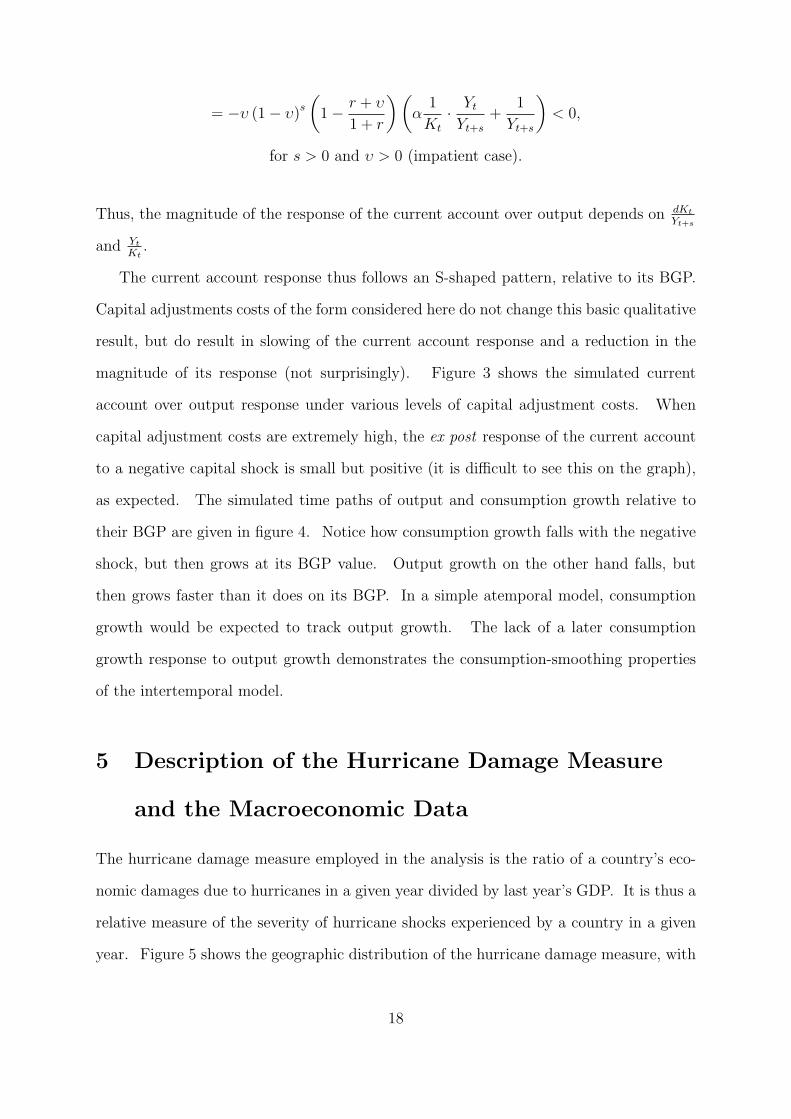
for s > 0 and υ > 0 (impatient case).
Thus, the magnitude of the response of the current account over output depends on dKt
Yt+s
and Yt
Kt.
The current account response thus follows an S-shaped pattern, relative to its BGP.
Capital adjustments costs of the form considered here do not change this basic qualitative
result, but do result in slowing of the current account response and a reduction in the
magnitude of its response (not surprisingly). Figure 3 shows the simulated current
account over output response under various levels of capital adjustment costs. When
capital adjustment costs are extremely high, the ex post response of the current account
to a negative capital shock is small but positive (it is difficult to see this on the graph),
as expected. The simulated time paths of output and consumption growth relative to
their BGP are given in figure 4. Notice how consumption growth falls with the negative
shock, but then grows at its BGP value. Output growth on the other hand falls, but
then grows faster than it does on its BGP. In a simple atemporal model, consumption
growth would be expected to track output growth. The lack of a later consumption
growth response to output growth demonstrates the consumption-smoothing properties
of the intertemporal model.
5 Description of the Hurricane Damage Measure
and the Macroeconomic Data
The hurricane damage measure employed in the analysis is the ratio of a country’s eco-
nomic damages due to hurricanes in a given year divided by last year’s GDP. It is thus a
relative measure of the severity of hurricane shocks experienced by a country in a given
year. Figure 5 shows the geographic distribution of the hurricane damage measure, with
18

each circle area indicative of the size of hurricane damages. Notice how the largest
hurricane shocks mostly occur in the small island economies of the Lesser Antilles. The
empirical cumulative distribution function for the hurricane damage measure is in figure
6. It shows how large hurricane shocks are relatively uncommon events.
The economic damage figures (all in current US$), primarily come from one of two
sources: annual articles on the Atlantic hurricane season in the American Meteorological
Society’s Monthly Weather Review ; or, the Emergency Events Database (EM-DAT) of
the World Health Organization’s Collaborating Centre for Research on the Epidemiol-
ogy of Disasters (CRED). In both cases, I compiled annual data on damages for the
period 1960 to 2002. Further data on economic damages were taken from a variety
of sources, including: the United Nations’ Economic Commission for Latin America
and the Caribbean (ECLAC), the US National Climatic Data Center (NCDC), the US
Agency for International Development’s Office of US Foreign Disaster Assistance (USAID
OFDA), the Inter-American Development Bank (IADB), the Meteorological Service of
the Netherlands Antilles and Aruba (MDNAA), Swiss Re, Grenada’s Ministry of Foreign
Affairs and International Trade, the Caribbean Disaster Emergency Response Agency
(CDERA), Guy Carpenter and Company Incorporated, and the United Nations’ Depart-
ment of Humanitarian Affairs (UNDHA).26
For those events for which no economic damage figure was available, I compared the
quality of damages in a country due to the storm event to other countries’ with a similar
damage pattern from other storm events, for which economic damage data exists.27 I then
inferred that the relative economic damage (described above) inflicted is likely similar for
these events. For example, in 1979, Hurricane David struck Dominica, leaving 80% of the
population homeless. Unfortunately, no valuations of the aggregate damage are available.
However, St. Lucia, a near neighbor of Dominica, also experienced a destruction of around
26Details on the exact construction of the dataset (e.g., which observations come from which source,etc.) are available upon request.
27Examples of measures of the quality of damages due to a hurricane include the death rate, proportionof the housing stock or buildings destroyed, proportion of the agricultural sector damaged and the sizeof the agricultural sector, infrastructure damage estimates, etc.
19

80% of its housing stock, when it was struck by Hurricane Allen in 1980 [Granger, 1990].
Economic damages for St. Lucia were 2.3 times annual GDP. Dominica likely had a
similar level of economic damages from Hurricane David. Accordingly, I use St. Lucia’s
relative economic damage measure from Hurricane Allen as a proxy for Dominica’s relative
economic damage from Hurricane David. Excluding such observations from the analysis
does not affect the estimated responses substantially.
Annual economic data are drawn from the World Development Indicators (WDI) 2003
dataset of the World Bank.28 The WDI is generally acknowledged to contain the most
reliable macroeconomic data for developing countries. The economic variables I look at
are:
1. the current account over GDP;
2. the gross national saving rate (inclusive of all income and transfers);
3. the gross investment rate (gross capital formation over GDP);
4. the log difference of per capita real GDP (measured in constant local currency
units);
5. the log difference of per capita real final consumption expenditures (measured in
constant local currency units);
6. the current account minus net transfers over GDP;
7. net unilateral transfers over GDP;
8. foreign aid over GDP;
9. worker remittances over GDP;
10. the overall government budget deficit over GDP.
28As far as I know, the data do not exist for the countries in my sample at a higher frequency.
20
The ICA model presented in Section 4 implies that the pure levels of all of the relevant
variables are nonstationary. Hence, stationary transformations (such as log differences
or ratios relative to GDP) of the pure levels are used in the analysis. In the empirical
analysis, all variables are converted to their percentage point equivalents for legibility
(viz., they have all been multiplied by 100).
I also investigated the effects of including various country-specific characteristics as
explanatory variables into the analysis. These are:
1. real GDP in the year prior to a shock (measured in constant 1995 US dollars);
2. bank-owned net foreign assets over GDP in the year prior to a shock (inclusive of
private and central bank deposits abroad);
3. external debt over GDP in the year prior to a shock;
4. agricultural value-added over GDP in the year prior to a shock (measuring the size
of the agricultural sector).
Countries included in the analysis are in the Caribbean and Central America. Essen-
tially, these are small countries which have some probability of experiencing a hurricane
strike. A list and description of the sample is found in Table 1. The time period
covers 1960 to 2002, all the years for which WDI data exist. Data availability is the
primary restriction for inclusion in the sample. As evinced by the table, the number of
observations available for each country (and variable) varies widely. The sample is thus
unbalanced.
6 Econometric Methodology – Panel Data Model
To uncover the response to a hurricane, I estimate a fixed effects panel regression mod-
els for each of the macroeconomic variables, delineated above. The general regression
21

equation is:
Yi,t = αi + βt +M∑
m=0
γmLmHi,t +M∑
m=0
Lm[
Hi,tX′i,t−1
]
δm + εi,t
where i indexes countries, t indexes year, Y denotes the macroeconomic variable of inter-
est, H denotes the relative economic damages due to a hurricane (defined earlier), X is
a (K × 1) vector of country-specific characteristics, and L is the standard lag operator.
ε is a mean zero disturbance term, which may be heteroskedastic and/or autocorrelated.
The country fixed effects, denoted αi, allow for country-specific trends in each of the
dependent variables. They also absorb any direct effects of time-invariant characteristics
of the countries considered. The time fixed effects, denoted βt, allow for a common
region-wide macroeconomic shock each year. The coefficient on the relative economic
damage measure γm measures the direct effect of the hurricane shock at time m after the
shock. The term X ′i,t−1δm measures the indirect effect of the hurricane shock at time
m, which depends upon country-specific characteristics in the year prior to a hurricane
shock.29 The regression is thus a distributed lag model, with lag length M . It measures
the reduced form effect of a hurricane, as I am not modelling the simultaneity among the
dependent variables. The above econometric model allows for a particularly rich impulse
response to a hurricane shock.
For each dependent variable, I tested a random effects specification versus a fixed ef-
fects specification, using the heteroskedasticity/autocorrelation robust test in Wooldridge
[2002]. The random effects specification is rejected for all of the variables. Furthermore,
tests of heteroskedasticity and autocorrelation of the error disturbances revealed that
these were present.30 Hence, I employ Newey-West heteroskedasticity and autocorrela-
tion robust (HAC) standard errors for all of the statistical inference. This allows for
arbitrary heteroskedasticity and autocorrelation, both within and across panels (coun-
29Lagged country-specific characteristics are used to mitigate endogeneity concerns.30Formal test results for the RE vs. FE, heteroskedasticity, and autocorrelation tests are available
upon request.
22
tries).
The choice of the lag length M for each equation is made using the joint hypothesis
testing procedure described in Pagano and Hartley’s [1981] article on fitting distributed
lag models.31 The maximum lag length considered is 10.
The empirical results presented derive from econometric models which impose various
restrictions on the above general model. The baseline specification imposes the restric-
tion that δm be equal to zero. It thus assumes that only the direct effects of the hurricane
are significant. In later specifications, I included the country-specific characteristic vari-
ables (elements of Xi,t). They are included singularly, as the introduction of multiple
characteristic variables with the lag structure rapidly burns up the degrees of freedom.
7 Empirical Results
Here, I discuss in greater detail the panel model results. In the first part of this section,
I present the baseline results, estimated under the restriction that δm = 0. In the second
part of this section, I introduce a set of country-specific characteristics and hurricane
damage measure interactions into the analysis, thus allowing for the economy’s response
to a hurricane shock to vary across country characteristics. Finally, I conclude this
section by considering the correspondence between the estimated response’s timing and
magnitude with that predicted by a standard ICA model.
7.1 Baseline Specification - Hurricane Damages Alone
Coefficient estimates in the baseline results may be interpreted as the dependent variable’s
response to a hurricane shock that destroys physical capital valued at one year’s national
GDP.32 The baseline results in table 2 show the expected intertemporal response of the
current account. There is a 5 percentage point fall in the current account over GDP in
31Lag truncation for the Newey-West HAC estimator is calculated by(
3
4
)
T( 1
3 )aver , and rounding up.
Taver is the average length of a panel. This results in a lag truncation parameter of 3 for all regressions.32Thus, −∆Kt
Yt
= 1.
23

the year after a hurricane shock, as expected in both the intertemporal and atemporal CA
models (significant at the 1% level). The S-shaped current account response predicted
by an ICA model is visible 3 years after a hurricane shock in the 2.7 percentage point
improvement, although significant only at the 10% level. In subsequent years, the point
estimates are all positive, although generally insignificant. However, they culminate
eight years after the hurricane shock in a 2.7 percentage point positive response which is
significant at the 5% level. Such a response is not consistent with an atemporal model.33
The gross national saving rate shows a large increase from 2 years after a hurricane
shock to 5 years after a hurricane shock. The size of the increase ranges from 5 percentage
points to 3.4 percentage points. Notice how the later year increases in saving are larger
than any of the contemporaneous increases in investment, likely generating the later
estimated positive response of the current account. Curiously, the gross saving rate in
the year of a hurricane shock shows an increase of 3.8 percentage points. This may be
related to a large influx of net transfers from abroad in the year of a hurricane shock.
Table 3 provides evidence that is weakly supportive of this hypothesis. Although there is
no significant foreign aid response contemporaneous with a hurricane shock, net transfers
over GDP does show a large response of 7.3 percentage points which is significant at the
10% level. Interestingly, net worker remittances received (a component of net transfers
exclusive of foreign aid) shows a 2.4 percentage point rise in the year of a hurricane shock
(significant at the 10% level). The rise in the annual saving rate in the year of a hurricane
shock could also reflect increased buffer-stock saving in anticipation of a hurricane shock.
The Atlantic basin hurricane season is most active from August to October. Thus,
higher than usual saving earlier in the year might more than offset later dissaving due
33I have not attempted to account for the possibility of insurance. If countries are insuring againststorm shocks, then one might be concerned that the observed current account response merely reflectsthe flows of insurance claims. However, insurance claims would enter positively into the current account,mitigating the current account response. Premiums paid out to foreign insurers are counted as importsof insurance service, and thus claims received count positively into the services portion of the currentaccount, acting similar to an income or transfer flow from abroad. In any case, it’s likely the case thatdeveloping countries are underinsured against such shocks. Even in the United States, it is estimatedthat insurance covers at best half of the actual damage caused by hurricanes [Pielke, Jr. and Landsea,1998].
24

to a hurricane, since hurricane shocks typically occur late in the year (the later third to
early fourth quarters of the calendar year). Quarterly data could resolve this puzzle, but
they are not available for the vast majority of countries in the sample.
The gross investment rate shows a strong positive response inclusive of the year of
the hurricane shock, which declines in magnitude over time. It ranges from 3.8 to 5.9
percentage points above its trend value up to 2 years after the hurricane shock, with the
largest response in the year just after the shock (all significant at the 1% level). The
response is smaller but positive in later years, culminating in an estimated 2 percentage
point rise above trend six years after the hurricane shock (significant at the 5% level).
This is consistent with a hurricane shock being a physical capital shock and not a pure
income shock (e.g., such as might be expected from a fall in tourism demand or the like).
Real output and consumption growth both show significant declines due to a hurricane
shock, although the declines are not synchronized. Output growth falls 5.4 percentage
points in the year of a hurricane shock (significant at the 5% level). Consumption growth
falls by 4.8 percentage points 2 years after a hurricane (significant at the 5% level),
recovering somewhat in the third year after a hurricane to 3.9 percentage points below its
trend value (significant at the 1% level. Perplexingly, the results show a 2.8 percentage
point rise in real consumption growth the year after a hurricane shock (significant at the
5% level). This is likely due to the inclusion of consumer durables, which can arguably
be considered investment goods, in the consumption measure. Unfortunately, the WDI
does not contain non-durable consumption with which to test this assertion. There
is a later real output growth increase of 3.7 percentage points above trend eight years
after the hurricane shock (significant at the 10% level), which is consistent with there
being some catch-up after a negative shock. However, real consumption growth shows
an unexpected rise of 4.3 and 4.9 percentage points above trend, nine and ten years after
a hurricane shock (significant at the 1% level). A rise in consumption growth is also
suggested by a decline in the gross national saving rate ten years after a hurricane shock
(-3.1 percentage points, significant at the 5% level).
25

As mentioned above, there is evidence of a net transfers’ response to a hurricane shock.
As seen in table 3, in the year after a hurricane shock, net transfers over GDP shows
an increase of 5.4 percentage points above trend (significant at the 5% level). This
response appears to be coming partially from increases in foreign aid (3.2 percentage
point increase, significant at the 5% level) and worker remittances (1.8 percentage point
increase, significant at the 10% level). When net transfers are subtracted from the current
account, the negative contemporaneous effect of a hurricane shock is even larger and more
significant, indicating that transfers from abroad dampen the effect of a hurricane shock
on the current account. However, the timing of large transfer flows does not coincide
with large movements in national saving or the current account, excepting the years
immediately following a hurricane shock. There is evidence of a 3.1 percentage point
increase in the overall government budget deficit over GDP 3 years after a hurricane
shock (significant at the 1% level). Again though, the gross national saving rate 3 years
after a hurricane shock still shows a positive significant response despite the fall in public
saving.34
7.2 Differential Responses across Country-specific Characteris-
tics
As described in the econometrics discussion, I also introduced several characteristic vari-
ables interacted with the hurricane damage measure as additional explanatory variables.
The variables I considered included: (1) economic size (real GDP); (2) bank-owned net
foreign assets over GDP; (3) external debt over GDP; and, (4) the size of the agricultural
sector (agricultural value-added over GDP). In my discussion, I focus on the estimated
current account responses.
34Although the baseline real ICA model makes no predictions about nominal prices, I also looked fora hurricane shock effect on CPI-measured inflation and the rate of foreign exchange rate depreciation.I found no significant effect on these variables. This likely reflects the fact that the small economies ofthe sample are price-takers in world markets. Furthermore, several of the countries in the sample arestrong fixers (e.g., the members of the East Caribbean Currency Union have never devalued/revaluedthe EC$).
26

Table 4 presents the estimated marginal effects of economic size, bank-owned net for-
eign assets over GDP and agricultural sector size upon the current account over GDP.
The effects are given for two levels (small and large; negative and positive; small and
large) of each characteristic variable. The results differentiated by country-specific char-
acteristics are more mixed than the baseline results. In part, this may reflect the loss
of degrees of freedom incurred by introducing another nine parameters to estimate in
the fixed effects framework. However, they do still suggest some kind of S-shaped re-
sponse, with earlier negative movements in the current account, followed by later positive
movements in the current account.
As seen in columns 1 and 2 of Table 4, there is little difference in the current account
response magnitude between small and large economies, for a hurricane shock of similar
relative size (capital destruction equal to 100% of annual GDP). The initial negative
response is present, but insignificant for both economic sizes (p-value of 0.107 for the small
economy case). Both do show a later positive move of the current account (significant
at the 1% level for the small economy and 10% for the large economy).
Columns 3 and 4 show that countries with negative bank-owned net foreign assets
(NFA) over GDP experience a larger negative move of the current account initially after
a hurricane shock (significant at the 10% level). Economies with negative bank-owned
NFA show a more dramatic S-shaped current account response than those with positive
bank-owned NFA.35 To the extent that bank-owned NFA reflect the overall economy’s
NFA, the results lend some support to Kraay and Ventura’s [2000] ICA model with
differential responses across creditor and debtor economies. However, given that the
coefficients are only significant at the 10% level, it can only be suggestive.
Economies with large agricultural sectors at the time of a hurricane shock show much
more dramatic negative early effects of a hurricane shock, as seen in columns 5 and 6.
This is not surprising, as extensive crop damage can appear even with storms which do not
generate large capital damages. The estimated current account decline in the year after
35The levels of NFA to GDP are both equal in magnitude to 5% of annual GDP.
27
a hurricane shock is -17.8 percentage points, significant at the 5% level. Furthermore,
their recovery is much more sluggish than that of economies with small agricultural
sectors. There is an eventual positive current account response for economies with large
agricultural sectors, but this appears only eight years after a hurricane shock (significant
at the 10% level).
External debt showed no relationship with the current account, although there are
few observations available for this variable.36
Despite the generally more imprecise estimates when conditioning upon country-
specific characteristics, all of the results do appear to show a later positive move of
the current account. Such an active response to a negative capital shock is required by
an intertemporal model, reflecting the interaction of the intertemporal budget constraint
and agent impatience.
8 Discussion and Implications
I now consider the the economic significance of the baseline results and their implications
for ICA models.
8.1 Economic Significance of the Baseline Estimates
What is the economic significance of these estimates? The average current account over
GDP from 1960 to 2002 is -7.45 percentage points. Thus, the estimated 5 percentage
point fall of the current account over GDP due to a hurricane shock means that the
current account worsens by some 70%, relative to its average value. Simulations of the
current account consequences of a hurricane shock generally show an even larger negative
contemporaneous response (see figure 3). However, as capital adjustment costs become
more important in the economy, the simulated response becomes smaller in magnitude.
The smaller estimated size of the current account response may thus be indicative of
36Available upon request.
28

significant capital adjustment costs at work in the economy. These may be either direct
(for example, if public infrastructure construction is a necessary pre-condition for pri-
vate capital investment to proceed), or indirect (for example, due to international capital
market imperfections). The estimated future 2.7 percentage point rise above trend of
the current account over GDP represents an improvement of 35% relative to its aver-
age value. The smaller magnitude of the future current account response relative to
the contemporaneous response is predicted by an ICA model with adjustment costs, as
illustrated by the simulated current account response mentioned above. The S-shaped
intertemporal response manifests with a lower amplitude.
Given that hurricane shocks generally occur in the last third of a year, the estimated
5.4 percentage point fall in real output growth due to a capital stock fall equal to one
year’s GDP is actually reflective of the growth rate in the last four months of the year.
The annualized real output growth rate (relative to trend) in the year’s last third is thus
around -13%, which is a substantial fall in income. The simulated fall in real output
growth relative to its BGP of -14% due to a 40% fall in the capital stock is remarkably
close to this figure (see figure 4).
8.2 Baseline Current Account Response Timing and Magnitude
The general qualitative characteristics of the estimated current account response match
the predictions of an ICA model. There is evidence of intertemporal trade occurring
in response to a negative capital shock. However, a comparison of the estimated re-
sponse’s timing and magnitudes with a standard ICA model’s predictions reveals some
discrepancies.
As seen in figure 3 and mentioned above, a standard ICA model predicts that the
current account over GDP will exhibit an extremely strong initial negative response to a
hurricane shock. There is then a much smaller, but more drawn out, positive response in
future periods. When there are no capital adjustment costs, the initial negative current
account response is approximately 6.75 times the size of the largest future positive current
29

account response. When capital adjustment costs are introduced, the size differential
becomes even greater. The estimated current account response (from table 2) shows a
size differential of only approximately 2. The empirical future current account response
is thus much stronger than that predicted by a standard ICA model.
In the absence of capital adjustment costs, the growth rate of the future current
account response is constant in a standard ICA model. The current account smoothly
declines, converging to its long-run value. When capital adjustment costs are present,
the growth rate of the future current account response takes on a hump-shaped pattern,
increasing slowly to a peak value and then decreasing. Again, the current account
smoothly converges to its long-run value. The estimated future current account response
does not appear to exhibit such smooth behaviour. However, the hypothesis that the
growth rate of the future current account response is constant cannot be rejected.37
The discrepancies between the estimated current account response and that predicted
by a standard ICA model suggest some possible modifications to the theory.38 First, the
ICA model simulated here is a perfect foresight model, where the negative capital shock
is unique and completely unexpected. Explicitly incorporating a buffer-stock savings
motive could help account for the stronger future current account response. Since there
is some probability of being struck by a damaging hurricane again, there is an incentive
to pay down debt more quickly than in the perfect foresight model. Second, there is
only a single asset (foreign bonds), which must be paid back only in the limit. Allowing
for a richer portfolio of assets which show a variety of maturity structures could also
help account for the discrepancies outlined above. The exact portfolio available depends
upon a country’s degree of international capital market access. Related to this, strategic
concerns on the part of either borrowers or lenders may also motivate a stronger future
current account response. Third, theoretical modifications which affect the smooth
37The delta-method is used to calculate the standard errors of the implied growth rates and then testthe non-linear (in parameters) hypothesis. The annual growth rates are calculated from the ex post
responses from year 3 to 8.38The following modifications maintain the fundamental structure of the problem, assuming a repre-
sentative agent and an invariant period utility function.
30

convergence (viz., adjustment behaviour) of the economy, such as the introduction of
nominal rigidities or habit formation, may help better match the estimated response.
Regardless, theoretical modifications must address the rate at which the intertemporal
budget constraint binds.
9 Conclusion
Many tests of the intertemporal approach to the current account rely upon the implicit
decomposition of shocks within a VAR framework. I argued that hurricanes represent
exactly the kinds of temporary, country-specific shocks required to test for an intertem-
poral trade response, obviating the need to extract shocks to macroeconomic variables
via a VAR model. With data on hurricane economic damages in Central America and
the Caribbean, I am able to quantify the size of the capital shock experienced by an
economy. I then used the hurricane damage measure to investigate the response of a
variety of macroeconomic variables, focusing on the behavior of the current account to
GDP ratio. The presence of capital adjustment costs implies that the macroeconomic re-
sponse to even a large capital shock will be somewhat muted, as costs are spread out over
time. This means that very large shocks, such as major hurricanes for small economies,
are likely needed to identify an intertemporal response.
The results show an S-shaped current account response which is consistent with an
intertemporal model but not an atemporal model. There is clear evidence of intertempo-
ral trade occurring. However, the response does not exhibit the smooth convergence and
exact timing expected by a standard ICA model, implying that theory must be modified
to address the rate at which the intertemporal budget constraint binds. In response to
a hurricane shock destroying capital equal to one year’s GDP, there is an initial move of
the current account to deficit relative to the BGP (-5 percentage points). This is later
reversed by a move to surplus relative to the BGP (+2.7 percentage points), which then
shrinks over time as the current account converges to its BGP value.
31
More broadly, the paper’s empirical findings indicate that the countries in the sample
are experiencing large wealth shocks from hurricanes, which entail costly reinvestment.
Underinsurance against hurricane losses results in further hardship, generating substan-
tial debt acquisition in response to a hurricane shock and reducing welfare by necessitating
buffer-stock saving. Small, island economies have no hinterland upon which to draw in
the event of a negative capital shock, and thus rely heavily upon the international com-
munity and international markets to aid their recovery [Fleming, 2004]. More complete
international insurance markets would mitigate both ex post debt acquisition and the ex
ante need for buffer-stock saving, improving welfare for these economies.
Finally, Gallup et al. [1998] argue that geography plays a large part in economic de-
velopment. Developing countries may be relatively poor in large part to their geographic
circumstances (for example, being landlocked or being subject to particularly malicious
disease organisms). The paper lends some support to this position. Hurricanes represent
large negative capital shocks which can consistently impoverish a country, potentially in-
hibiting its ability to develop.39 Geography has placed the countries of the Caribbean
and Central America in the path of many of these damaging storms. Furthermore, the
evidence suggests that the countries of the Caribbean and Central America are becoming
more vulnerable to hurricane shocks as a consequence of increased coastal and moun-
tainous regional development, poor building construction, and deforestation [Pielke, Jr.
et al., 2003]. If such a trends continue, the effects of hurricanes upon development will
only become larger.
39For an argument against this interpretation, see Skidmore and Toya [2002]. They argue that a highincidence of natural disasters is associated with higher total factor productivity and economic growth,by encouraging human capital investment and the adoption of new, more productive vintages of physicalcapital.
32

References
Shaghil Ahmed. Temporary and permanent government spending in an open economy:Some evidence for the United Kingdom. Journal of Monetary Economics, 17:197–224,1986.
Shaghil Ahmed. Government spending, the balance of trade, and the terms of trade inbritish history. Journal of Monetary Economics, 17:197–224, 1987.
John Y. Campbell. Does saving anticipate declining labor income? An alternative testof the permanent income hypothesis. Econometrica, 55:1249–1273, 1987.
Christopher Carroll. Theoretical foundations of buffer stock saving. NBER Working
Paper, (10867), October 2004.
Giancarlo Corsetti and Panagiotis T. Konstantinou. The dynamics of the U.S. net foreignliabilities: an empirical characterization. photocopy, European University Instituteand University of Rome III, 2004.
Angus Deaton. Saving in developing countries: Theory and review. In Proceedings of the
World Bank Annual Conference on Development Economics 1989, pages 61–96, 1990.
James B. Elsner and A. Birol Kara. Hurricanes of the North Atlantic: Climate and
Society. Oxford University Press, New York, NY, 1999.
Martin Feldstein and Charles Horioka. Domestic saving and international capital flows.Economic Journal, 90:314–329, 1980.
Charles Fleming. Unmatched scope of disaster delays damage estimates. Wall Street
Journal, page A8, December 28 2004.
John Luke Gallup, Jeffrey D. Sachs, and Andrew D. Mellinger. Geography and economicdevelopment. NBER Working Paper, (6849), 1998.
Atish R. Ghosh. Capital mobility amongst the major industrialized countries: Too littleor too much. Economic Journal, 105:107–128, 1995.
Atish R. Ghosh and Jonathan D. Ostry. The current account in developing countries: Aperspective from the consumption-smoothing approach. World Bank Economic Review,9:305–333, 1995.
Domenico Giannone and Michele Lenza. The Feldstein-Horioka fact. CEPR Discussion
Paper, (4610), 2004.
Reuven Glick and Kenneth Rogoff. Global versus country-specific productivity shocksand the current account. Journal of Monetary Economics, 35:159–192, 1995.
Pierre-Olivier Gournichas and Helene Rey. International financial adjustment. NBER
Working Paper, (11155), 2005.
Orman E. Granger. Natural Disasters and Social Change: An Eastern Caribbean Per-
spective. University of California-Berkeley, Berkeley, CA, 1990.
33

Lars P. Hansen and Thomas J. Sargent. Two difficulties in interpreting vector autore-gressions. In Lars P. Hansen and Thomas J. Sargent, editors, Rational Expectations
Econometrics, Underground Classics in Economics. Westview Press, 1991.
Mathias Hoffmann. The relative dynamics of investment and the current account in theG7-economies. Economic Journal, 111:C148–C163, May 2001.
Mathias Hoffmann. International macroeconomic fluctuations and the current account.Canadian Journal of Economics, 36(2):401–420, May 2003.
Kenneth Kasa. Testing present value models of the current account: a cautionary note.Journal of International Money and Finance, 22:557–569, 2003.
Aart Kraay and Jaume Ventura. Current accounts in debtor and creditor countries.Quarterly Journal of Economics, 115(4):1137–1166, November 2000.
Aart Kraay and Jaume Ventura. Current accounts in the long and short run. In MarkGertler and Kenneth Rogoff, editors, 2002 NBER Macroeconomics Annual, chapter 2.MIT Press, Cambridge, MA, 2003.
Christopher W. Landsea, Roger A. Pielke, Jr., Alberto M. Mestas-Nunez, and John A.Knaff. Atlantic Basin Hurricanes: Indices of Climatic Changes. Climatic Change, 42:89–129, 1999.
Philip R. Lane. The new open economy macroeconomics: A survey. Journal of Interna-
tional Economics, 54:235–266, 2001.
James M. Nason and John H. Rogers. The present-value model of the current accounthas been rejected: Round up the usual suspects. Federal Reserve Board of Governors
International Finance Discussion Paper, (760), 2003.
Maurice Obstfeld. External adjustment. NBER Working Paper, (10843), 2004.
Maurice Obstfeld and Kenneth Rogoff. The intertemporal approach to the current ac-count. In Gene M. Grossman and Kenneth Rogoff, editors, Handbook of International
Economics, volume 3 of Handbooks in economics, chapter 34, pages 1731–1799. ElsevierScience B.V., Amsterdam, 1995.
Maurice Obstfeld and Kenneth Rogoff. Foundations of International Macroeconomics.MIT Press, Cambridge, Massachusetts, first edition, 1996. ISBN 0262150476.
Glenn Otto. Testing a present-value model of the current account: Evidence from USand Canadian time series. Journal of International Money and Finance, 11:414–430,1992.
Marcello Pagano and Michael J. Hartley. On fitting distributed lag models subject topolynomial restrictions. Journal of Econometrics, 16:171–198, 1981.
Roger A. Pielke, Jr. and Christopher W. Landsea. Normalized hurricane damages in theUnited States: 1925-1995. Weather and Forecasting, 13:621–631, 1998.
34
Roger A. Pielke, Jr. and Roger A. Pielke, Sr. Hurricanes, Their Nature and Impacts on
Society. John Wiley and Sons, New York, NY, 1997.
Roger A. Pielke, Jr., Jose Rubiera, Christopher Landsea, Merio L. Fernandez, andRoberta Klein. Hurricane vulnerability in Latin America and the Caribbean: Nor-malized damage and loss potentials. Natural Hazard Review, 4(3):101–114, August2003.
Steven M. Sheffrin and Wing Thye Woo. Present value tests of an intertemporal modelof the current account. Journal of International Economics, 29:237–253, 1990.
Mark Skidmore and Hideki Toya. Do natural disasters promote long-run growth? Eco-
nomic Inquiry, 40(4):664–687, October 2002.
Cedric Tille. Financial integration and the wealth effect of exchange rate fluctuations.Photocopy, Federal Reserve Bank of New York, August 2004.
Jeffrey M. Wooldridge. Econometric Analysis of Cross Section and Panel Data. MITPress, Cambridge, Massachusetts, first edition, 2002. ISBN 0262232197.
35

Data Sources
Associated Press. Damage in Dominican Republic above $1 billion. Associated PressWire Report, September 1998.
Lixion A. Avila and Edward N. Rappaport. Atlantic Hurricane Season of 1994. Monthly
Weather Review, 124:1558–1578, 1996.
Lixion A. Avila and Edward N. Rappaport. Atlantic Hurricane Season of 1996. Monthly
Weather Review, 127:581–610, 1999.
John L. Beven II, Stacy R. Stewart, Miles B. Lawrence, Lixion A. Avila, James L.Franklin, and Richard J. Pasch. Atlantic Hurricane Season of 2001. Monthly Weather
Review, 131:1454–1484, July 2003.
Robert A. Case. Atlantic Hurricane Season of 1985. Monthly Weather Review, 114:1390–1405, 1986.
Robert A. Case and Harold P. Gerrish. Atlantic Hurricane Season of 1983. Monthly
Weather Review, 112:1083–1092, 1984.
Robert A. Case and Harold P. Gerrish. Atlantic Hurricane Season of 1987. Monthly
Weather Review, 116:939–949, 1988.
Robert A. Case and Max Mayfield. Atlantic Hurricane Season of 1989. Monthly Weather
Review, 118:1165–1177, May 1990.
Caribbean Disaster Emergency Response Agency. Tropical storm Lili situation reportno. 2. Technical Report 2, Caribbean Disaster Emergency Response Agency, October2002.
Gilbert B. Clark. Atlantic Hurricane Season of 1982. Monthly Weather Review, 111:1071–1079, 1983.
Centre for Research on the Epidemiology of Disasters. EM-DAT: the OFDA/CREDinternational disaster database. Website, 2004. URL http://www.em-dat.net.
Department of Regional Development and Environment Executive Secretariat for Eco-nomic and Social Affairs. Primer on Natural Hazard Management in Integrated Re-
gional Development Planning. Organization of American States, Washington, D.C.,1991.
Gordon E. Dunn. The Hurricane Season of 1960. Monthly Weather Review, pages 99–108,March 1961.
Gordon E. Dunn and Staff. The Hurricane Season of 1961. Monthly Weather Review,pages 107–119, March 1962.
Gordon E. Dunn and Staff. The Hurricane Season of 1962. Monthly Weather Review,pages 199–207, April 1963.
36

Gordon E. Dunn and Staff. The Hurricane Season of 1963. Monthly Weather Review, 92(3):128–138, March 1964.
Gordon E. Dunn and Staff. The Hurricane Season of 1964. Monthly Weather Review, 93(3):175–187, March 1965.
Economic Commission for Latin America and the Caribbean. Preliminary overview ofthe economies of Latin America and the Caribbean 1998. Technical report, UnitedNations’ Economic Commission for Latin America and the Caribbean, December 1998.
Economic Commission for Latin America and the Caribbean. Costa Rica: Assessmentof the damage caused by Hurricane Mitch, 1998. Technical Report LC/MEX/L.373,United Nations’ Economic Commission for Latin America and the Caribbean, April1999a.
Economic Commission for Latin America and the Caribbean. El Salvador: Assessmentof the damage caused by Hurricane Mitch, 1998. Technical Report LC/MEX/L.371,United Nations’ Economic Commission for Latin America and the Caribbean, April1999b.
Economic Commission for Latin America and the Caribbean. Guatemala: Assessmentof the damage caused by Hurricane Mitch, 1998. Technical Report LC/MEX/L.370,United Nations’ Economic Commission for Latin America and the Caribbean, April1999c.
Economic Commission for Latin America and the Caribbean. Honduras: Assessmentof the damage caused by Hurricane Mitch, 1998. Technical Report LC/MEX/L.367,United Nations’ Economic Commission for Latin America and the Caribbean, April1999d.
Economic Commission for Latin America and the Caribbean. Nicaragua: Assessmentof the damage caused by Hurricane Mitch, 1998. Technical Report LC/MEX/L.372,United Nations’ Economic Commission for Latin America and the Caribbean, April1999e.
Economic Commission for Latin America and the Caribbean. Belize: Assessment ofthe damage caused by Hurricane Keith, 2000. Technical Report LC/CAR/G.627,LC/MEX/G.4, United Nations’ Economic Commission for Latin America and theCaribbean, November 2000.
Economic Commission for Latin America and the Caribbean. Jamaica: Assessment ofthe damage caused flood rains and landslides in association with Hurricane Michelle,october 2001. Technical Report LC/CAR/G.672, United Nations’ Economic Commis-sion for Latin America and the Caribbean, December 2001.
Economic Commission for Latin America and the Caribbean. Handbook for Estimating
the Socio-economic and Environmental Effects of Disasters. Number LC/MEX/G.5,LC/L.1874. United Nations, July 2003.
37

James L. Franklin, Lixion A. Avila, Jack L. Beven, Miles B. Lawrence, Richard J. Pasch,and Stacy R. Stewart. Atlantic Hurricane Season of 2000. Monthly Weather Review,129:3037–3056, 2001.
Paul J. Hebert. Atlantic Hurricane Season of 1975. Monthly Weather Review, 104:453–465, 1976.
Paul J. Hebert. Atlantic Hurricane Season of 1979. Monthly Weather Review, 108:973–990, 1980.
Paul J. Hebert and Neil L. Frank. Atlantic Hurricane Season of 1973. Monthly Weather
Review, 102:280–289, 1974.
John R. Hope. Atlantic Hurricane Season of 1974. Monthly Weather Review, 103:285–293,1975.
Miles B. Lawrence. Atlantic Hurricane Season of 1976. Monthly Weather Review, 105:497–507, 1977.
Miles B. Lawrence. Atlantic Hurricane Season of 1977. Monthly Weather Review, 106:534–545, 1978.
Miles B. Lawrence. Atlantic Hurricane Season of 1978. Monthly Weather Review, 107:477–491, 1979.
Miles B. Lawrence. Atlantic Hurricane Season of 1986. Monthly Weather Review, 115:2155–2160, September 1987.
Miles B. Lawrence, Lixion A. Avila, Jack L. Beven, James L. Franklin, John L. Guiney,and Richard J. Pasch. Atlantic Hurricane Season of 1999. Monthly Weather Review,129:3057–3084, 2001.
Miles B. Lawrence and Gilbert B. Clark. Atlantic Hurricane Season of 1984. Monthly
Weather Review, 113:1228–1237, 1985.
Miles B. Lawrence and James M. Gross. Atlantic Hurricane Season of 1988. Monthly
Weather Review, 117:2248–2259, October 1989.
Miles B. Lawrence, Max Mayfield, Lixion A. Avila, Richard J. Pasch, and Edward N.Rappaport. Atlantic Hurricane Season of 1995. Monthly Weather Review, 126:1124–1151, May 1998.
Miles B. Lawrence and Joseph M. Pelissier. Atlantic Hurricane Season of 1980. Monthly
Weather Review, 109:1567–1582, 1981.
Miles B. Lawrence and Joseph M. Pelissier. Atlantic Hurricane Season of 1981. Monthly
Weather Review, 110:852–866, 1982.
Max Mayfield, Lixion A. Avila, and Edward N. Rappaport. Atlantic Hurricane Seasonof 1992. Monthly Weather Review, 122:517–538, 1994.
38

Max Mayfield and Miles B. Lawrence. Atlantic Hurricane Season of 1990. Monthly
Weather Review, 119:2014–2026, 1991.
Meteorological Service of the Netherlands Antilles and Aruba. Prelim-inary report Hurricane Jose October 1999. Technical report, Meteo-rological Service of the Netherlands Antilles and Aruba, 2000. URLhttp://www.meteo.an/meteo2/eng/reports/jose/jose.htm.
U.S. National Climatic Data Center. Mitch: The Deadliest Atlantic Hurricanesince 1780. Technical report, U.S. National Climatic Data Center, 2004. URLhttp://lwf.ncdc.noaa.gov/oa/reports/mitch/mitch.html.
U.S. National Hurricane Center. Atlantic tracks file 1851-2003. Website, 2003. URLhttp://www.nhc.noaa.gov/tracks1851to2003 atl.txt.
Richard J. Pasch and Lixion A. Avila. Atlantic Hurricane Season of 1991. Monthly
Weather Review, 120:2671–2687, 1992.
Richard J. Pasch, Lixion A. Avila, and John L. Guiney. Atlantic Hurricane Season of1998. Monthly Weather Review, 129:3085–3123, 2001.
Richard J. Pasch, Miles B. Lawrence, Lixion A. Avila, John L. Beven, James L. Franklin,and Stacy R. Stewart. Atlantic Hurricane Season of 2002. Monthly Weather Review,132:1829–1859, July 2004.
Richard J. Pasch and Edward N. Rappaport. Atlantic Hurricane Season of 1993. Monthly
Weather Review, 123:871–886, 1995.
Edward N. Rappaport. Atlantic Hurricane Season of 1997. Monthly Weather Review,127:2012–2026, 1999.
Robert H. Simpson and Paul J. Hebert. Atlantic Hurricane Season of 1972. Monthly
Weather Review, 101:323–333, 1973.
Robert H. Simpson and John R. Hope. Atlantic Hurricane Season of 1971. Monthly
Weather Review, 100:256–267, 1972.
Robert H. Simpson and Joseph M. Pelissier. Atlantic Hurricane Season of 1970. Monthly
Weather Review, 99:269–277, April 1971.
Robert H. Simpson, Arnold L. Sugg, and Staff. The Hurricane Season of 1969. Monthly
Weather Review, 98(4):293–306, March 1970.
Arnold L. Sugg. The Hurricane Season of 1965. Monthly Weather Review, 94(3):183–191,March 1966.
Arnold L. Sugg. The Hurricane Season of 1966. Monthly Weather Review, 95(3):131–142,March 1967.
Arnold L. Sugg and Paul J. Hebert. The Hurricane Season of 1968. Monthly Weather
Review, 97(3):225–239, March 1969.
39

Arnold L. Sugg and Joseph M. Pelissier. The Hurricane Season of 1967. Monthly Weather
Review, 96(4):242–250, April 1968.
Swiss Re Economic Research and Consulting Sigma Series. Natural catastrophes andman-made disasters 1999: Storms and earthquakes lead to the second-highest lossesin insurance history. Technical Report 2/2000, Swiss Re, Zurich, Switzerland, 2000.
Swiss Re Economic Research and Consulting Sigma Series. Natural catastrophes andman-made disasters in 2002: high flood loss burden. Technical Report 2/2003, SwissRe, Zurich, Switzerland, 2003.
United Nations Department of Humanitarian Affairs. Dominica - Hurricane situationreport No. 3. Technical Report DHAGVA - 95/0421, United Nations Department ofHumanitarian Affairs, September 1995.
U.S. Agency for International Development. Caribbean, Dominican Republic, Haiti Hurri-cane Georges fact sheet #3. Technical report, U.S. AID, Office of U.S. Foreign DisasterAssistance, September 1998a.
U.S. Agency for International Development. Central America - Hurricane Mitch factsheet #21. Technical report, U.S. AID, Office of U.S. Foreign Disaster Assistance,December 1998b.
U.S. Agency for International Development. Northeastern Caribbean Hurricane Lennyfact sheet #1, FY 2000. Technical report, U.S. AID, Office of U.S. Foreign DisasterAssistance, November 1999.
U.S. Agency for International Development. Hurricane Lenny recovery in the EasternCaribbean. Special objective document, U.S. AID, Office of U.S. Foreign DisasterAssistance, April 2000.
World Bank. World Development Indicators. electronic dataset, 2003.
40

Table 1: Caribbean and Central American Sample Statistics (Annual Averages over 1960-2002)
Real GDP Real P.C. Bank-owned Net Agric. Sector Average(Millions of GDP (Cons. Population External Debt Foreign Assets Size (Prop. Number
Country Cons. 1995 US$) 1995 US$) (Thousands) over GDP over GDP of GDP) of Obs.St. Vincent and
the Grenadines $155 $1,483 98 28% 18% 15% 27St. Kitts and Nevis $186 $4,355 45 33% 18% 9% 23Dominica $190 $2,611 70 51% 5% 26% 23Grenada $244 $2,590 94 45% 11% 15% 24Belize $338 $1,939 158 40% 6% 22% 24St. Lucia $439 $3,133 120 23% 8% 12% 22Antigua and Barbuda $419 $6,481 63 - 4% 5% 23Bermuda $1,473 $33,008 63 - - - 5Barbados $1,516 $5,997 250 - 5% 10% 31Nicaragua $1,938 $673 3,147 276% -118% 26% 35Bahamas $2,540 $11,774 215 - -3% 2% 24Honduras $2,648 $655 3,926 74% 3% 27% 33Haiti $2,734 $497 5,667 29% 2% - 35Trinidad and Tobago $4,285 $3,789 1,096 28% 17% 4% 34Jamaica $4,314 $1,995 2,153 87% -5% 8% 29Panama $5,477 $2,607 2,003 76% -3% 8% 29El Salvador $7,139 $1,577 4,499 33% 1% 29% 35Costa Rica $7,381 $2,828 2,452 58% 5% 21% 35Dominican Republic $8,488 $1,333 5,874 37% -1% 17% 37Guatemala $10,120 $1,336 7,325 21% 4% 26% 33Puerto Rico $26,460 $7,958 3,181 - - 2% 11Mexico $206,700 $2,841 68,729 37% 4% 9% 34Aruba - - 87 - 20% - 4Cuba - - 9,593 - - 7% 2Netherlands Antilles - - 177 - 16% - 4US Virgin Islands - - 87 - - - 2
All statistics are sample annual averages by country over the period 1960-2002. The average number of observations is calculated from the total number of observations available forthe dependent variables in tables 2 and 3.
41

Table 2: Baseline Fixed Effects Panel Estimation Coefficients (Newey-West HAC Robust Standard Errors)
Dependent Variable
Current Account Gross Nat’l Gross Inv’t Real Output Real Cons.Explanatory Variable over GDP Saving Rate Rate Growth GrowthHurricane Damage 0.942 3.837∗∗ 5.134∗∗∗ -5.428∗∗ -0.815Measure (3.374) (1.652) (1.225) (2.218) (1.563)
Hurricane Damage L1 -5.043∗∗∗ 0.347 5.916∗∗∗ 0.394 2.811∗∗
(1.272) (1.514) (2.096) (1.372) (1.390)
Hurricane Damage L2 -1.588 3.393∗∗∗ 3.796∗∗∗ -0.815 -4.819∗∗
(1.096) (1.296) (0.980) (1.794) (2.464)
Hurricane Damage L3 2.738∗ 5.099∗∗∗ 1.863∗ 1.042 -3.903∗∗∗
(1.617) (1.459) (1.132) (0.886) (1.460)
Hurricane Damage L4 2.312 4.156∗∗∗ 1.297 2.233 4.248(1.919) (1.517) (1.212) (1.779) (2.839)
Hurricane Damage L5 1.636 4.499∗∗∗ 2.644∗∗ -1.366 -0.536(1.207) (0.917) (1.336) (1.180) (2.659)
Hurricane Damage L6 1.123 1.835 2.073∗∗ 0.258 2.440(1.838) (1.329) (0.817) (1.534) (1.421)
Hurricane Damage L7 1.091 -1.915 -0.630 0.689(1.684) (2.139) (0.920) (1.605)
Hurricane Damage L8 2.718∗∗ 1.486 3.747∗ -0.261(1.113) (1.184) (2.284) (1.928)
Hurricane Damage L9 0.548 4.306∗∗∗
(1.422) (1.612)
Hurricane Damage L10 -3.125∗∗ 4.982∗∗∗
(1.319) (1.880)
N 541 500 644 711 526R2 0.543 0.490 0.626 0.161 0.192
Significance levels: ∗ : 10% ∗∗ : 5% ∗ ∗ ∗ : 1%. Standard errors are underneath coefficient estimates in parentheses. “L” (for lag) followed by a number denotes the numberof years elapsed since a hurricane strike. The lag truncation parameter used is 3.
42

Table 3: Transfers and the Government – Fixed Effects Panel Estimation Coefficients (Newey-West HAC Robust StandardErrors)
Dependent Variable
Curr. Acc. minus Net Net Transfers Foreign Aid Workers’ Remit. Overall Gov’t Bud.Explanatory Variable Transfers over GDP over GDP over GDP over GDP Deficit over GDPHurricane Damage -6.389∗∗∗ 7.331∗ 0.992 2.396∗ -0.833Measure (1.775) (4.266) (0.984) (1.238) (0.865)
Hurricane Damage L1 -10.459∗∗∗ 5.416∗∗ 3.175∗∗ 1.766∗ 0.900(2.430) (2.554) (1.564) (0.917) (1.108)
Hurricane Damage L2 -5.135∗∗∗ 3.547∗∗∗ 1.290 1.021 -0.493(1.485) (1.314) (1.182) (0.800) (1.260)
Hurricane Damage L3 1.603 1.135 2.229∗ 0.776 3.107∗∗∗
(1.615) (1.488) (1.283) (0.670) (0.918)
Hurricane Damage L4 1.319 0.993 0.054 1.050(1.971) (1.240) (0.732) (0.855)
Hurricane Damage L5 0.132 1.504 -0.421 0.420(1.531) (1.173) (1.158) (0.935)
Hurricane Damage L6 0.369 0.755 -0.473 2.137∗∗∗
(1.791) (1.474) (1.094) (0.592)
Hurricane Damage L7 2.817 -1.726 0.426(1.810) (1.356) (0.925)
Hurricane Damage L8 4.187∗∗∗ -1.469∗ 1.675(1.415) (0.857) (1.039)
N 541 541 663 455 393R2 0.654 0.463 0.493 0.647 0.394
Significance levels: ∗ : 10% ∗∗ : 5% ∗ ∗ ∗ : 1%. Standard errors are underneath coefficient estimates in parentheses. “L” (for lag) followed by a number denotes the numberof years elapsed since a hurricane strike. The lag truncation parameter used is 3. Foreign aid is official development assistance. All other transfers are non-governmental, includingworker remittances.
43

Table 4: Marginal Effects of Hurricane Shocks on the Current Account over GDP (Newey-West HAC Robust Standard Errors)
Characteristic Variable and its Level
GDP GDP NFA NFA Agric. Agric.Explanatory Variable (Small) (Large) (Negative) (Positive) (Small) (Large)Hurricane Damage 0.098 -1.883 -1.896 0.548 3.421 -6.121Measure (2.807) (3.724) (2.811) (2.549) (3.858) (6.700)
Hurricane Damage L1 -4.446 -3.194 -6.223∗ -3.666 1.193 -17.776∗∗
(2.764) (3.687) (3.315) (2.865) (4.135) (9.014)
Hurricane Damage L2 0.615 -2.899 1.926 1.768 0.156 -0.812(2.356) (2.893) (2.990) (2.603) (3.787) (5.304)
Hurricane Damage L3 5.140 -0.647 6.101∗ 5.976∗ 2.345 3.866(3.638) (2.689) (3.585) (3.399) (5.629) (6.733)
Hurricane Damage L4 3.515 -2.204 6.493∗ 5.401 3.575 -0.309(4.247) (3.803) (3.674) (3.544) (5.747) (6.985)
Hurricane Damage L5 6.078∗ 1.911 3.061 6.773∗ 12.383∗∗ -10.365(3.574) (3.904) (4.112) (3.931) (5.124) (7.092)
Hurricane Damage L6 0.081 0.213 0.818 1.448 8.759 -18.058∗∗
(4.418) (4.518) (5.324) (4.381) (6.495) (9.120)
Hurricane Damage L7 1.546 4.885∗ 3.272∗ 2.413 -2.961 1.244(2.616) (2.599) (1.951) (2.529) (4.503) (1.904)
Hurricane Damage L8 4.269∗∗∗ 4.442∗ 2.741∗ 3.234∗ 2.098 2.492∗
(1.586) (2.617) (1.565) (1.739) (2.355) (1.355)
Significance levels: ∗ : 10% ∗∗ : 5% ∗ ∗ ∗ : 1%. Standard errors are underneath coefficient estimates in parentheses. L” (for lag) followed by a number denotes the numberof years elapsed since a hurricane strike. The characteristic variables are economic size (GDP), bank-owned net foreign assets (NFA), and size of the agricultural sector (Agric.).Small economic size corresponds to a real GDP level of $155 million, the time average of St. Kitt’s and Nevis’ real GDP. Medium economic size corresponds to a real GDP level of$2.54 billion, the time average of Guatemala’s real GDP. Negative NFA corresponds to a bank-owned net foreign assets to GDP ratio of -5%, the time average of Jamaica. PositiveNFA corresponds to a bank-owned net foreign assets to GDP ratio of +5%, the time average of Dominica or Costa Rica. Small agricultural sector size corresponds to 2% of GDP,the time average of the Bahamas. Large agricultural sector size corresponds to 29% of GDP, the time average of El Salvador. The lag truncation parameter used is 3.
44

Figure 1: Hurricane Incidence
020
4060
80N
umbe
r of
Sto
rms
1960 1965 1970 1975 1980 1985 1990 1995 2000
Source: US National Hurricane Center Historic Storm Tracks Database
1960−2003, Quintennial Totals
Annual Storm Incidencein the North Atlantic and Caribbean
Weak Tropical Storm Strong Tropical StormS−S Hurricane 1 S−S Hurricane 2S−S Hurricane 3 S−S Hurricane 4S−S Hurricane 5
45
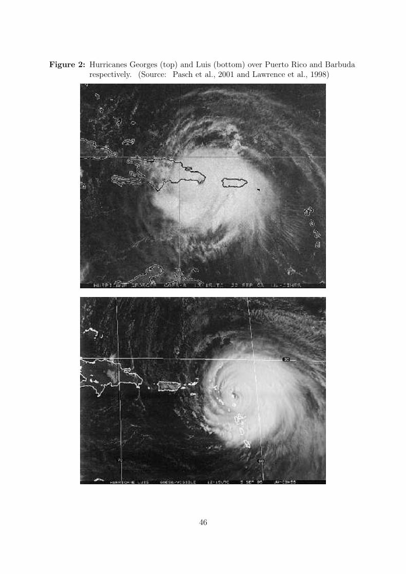
Figure 2: Hurricanes Georges (top) and Luis (bottom) over Puerto Rico and Barbudarespectively. (Source: Pasch et al., 2001 and Lawrence et al., 1998)
46

Figure 3: Simulated Impulse Response – Current Account over Output
−12
5−
100
−75
−50
−25
025
Rel
ativ
e to
Bal
ance
d G
row
th P
ath
0 1 2 3 4 5 6 7 8 9 10Time (Shock at t = 1)
No Adjustment Costs Chi = 0.1Chi = 0.2 Chi = 0.5
Per
cent
age
Poi
nt R
espo
nse
(40% of Physical Capital Stock Destroyed)Current Account to GDP Ratio Response
The deep parameter values underlying the above simulation are: real foreign interest rate r = 0.10; time discount factor β = 0.80; intertemporal elasticity of substitution σ = 2;Cobb-Douglas capital exponent α = 0.25; and exogenous rate of productivity growth g = 0.02. The parameter χ determines how large capital adjustment costs are, with highervalues implying larger costs (χ = 0 with no adjustment costs).
47

Figure 4: Simulated Impulse Responses – Output and Consumption Growth
−15
−10
−5
05
1015
Rel
ativ
e to
Bal
ance
d G
row
th P
ath
0 1 2 3 4 5 6 7 8 9 10Time (Shock at t = 1)
No Adjustment Costs Chi = 0.1Chi = 0.2 Chi = 0.5
Per
cent
age
Poi
nt R
espo
nse
(40% of Physical Capital Stock Destroyed)Real Output Growth Response
−20
−15
−10
−5
05
10R
elat
ive
to B
alan
ced
Gro
wth
Pat
h
0 1 2 3 4 5 6 7 8 9 10Time (Shock at t = 1)
No Adjustment Costs Chi = 0.1Chi = 0.2 Chi = 0.5
Per
cent
age
Poi
nt R
espo
nse
(40% of Physical Capital Stock Destroyed)Real Consumption Growth Response
The deep parameter values underlying the above simulation are: real foreign interest rate r = 0.10; time discount factorβ = 0.80; intertemporal elasticity of substitution σ = 2; Cobb-Douglas capital exponent α = 0.25; and exogenous rate ofproductivity growth g = 0.02. The parameter χ determines how large capital adjustment costs are, with higher valuesimplying larger costs (χ = 0 with no adjustment costs).
48

Figure 5: Caribbean and Central American Hurricane Damages Map
Colombia
Aruba
Antigua and Barbuda
Anguilla
Barbados
Bahamas
Belize
Cayman Islands
Costa Rica
Cuba
Dominica
Dominican Republic
El Salvador
Grenada
GuadeloupeGuatemala
Guyana
Haiti
Honduras
Jamaica
Martinique
Mexico
Nicaragua
Panama
Saint Lucia
Trinidad and Tobago
Turks and Caicos Islands
Venezuela
United States
Hurricane Relative Damage MeasureEconomic Damages over GDP
2.3
1.15
0.23
HURRICANE ECONOMIC DAMAGES BY COUNTRY:
1960-2003
49

Figure 6: Hurricane Damage Measure Distribution
.2.4
.6.8
1C
umul
ativ
e P
roba
bilit
y
0 .5 1 1.5 2 2.5Relative Damage Measure
Note: Underlying data are the annual maximum relative damagemeasure for each country in each year.
1960−2003
Empirical Cumulative Distributionof Relative Damage Measure
50

Appendix (NOT FOR PUBLICATION)
A Intertemporal Current Account Model Solution
Let Home’s small, open economy be characterized by a representative agent, who faces
the following problem:
maxCs,Is
U = Et
[
∞∑
s=t
βs−tu (Cs)
]
s.t. Cs = (1 + r) Bs + Ys + Ns − Is − C (Is, Ks) − Gs − Bs+1 for all s,
Ks+1 = (1 − εs+1) [Ks + Is] , Ks+1 = Ks + Is, Ys ≡ F (As, Ks) and As+1 = (1 + g) As.
Assume that the government budget is balanced (expenditures equal lump-sum tax re-
ceipts). The components of the problem are:
1. β is the time preference discount factor and β ∈ (0, 1) .
2. u (·) is a concave, period utility function.
3. C is period consumption.
4. B is net foreign asset holdings.
5. r is the exogenous constant foreign rate of return on foreign assets.
6. Y is output.
7. N is exogenous net transfers from abroad.
8. A is exogenous total factor productivity, which grows at rate g.
9. F (·) is a concave, linearly homogenous production function with FA > 0, FK > 0,
FAK > 0, FAA < 0, FKK < 0.
10. K is the physical capital stock (which is non-tradeable).
51

11. I is physical capital investment.
12. K is next period’s planned physical capital stock.
13. ε is the proportion of the planned physical capital stock that is destroyed in a
period, before it can be used in production.
14. C (I,K) is a convex, linearly homogenous physical capital adjustment cost function
with CI > 0, CK < 0, CII > 0, CKK > 0, C (0, Ks) = 0.
15. G is exogenous government spending.
The above represents the most general formulation of the intertemporal current account
model I will investigate. The general model implicitly assumes that international asset
markets are incomplete (a complete set of state-contingent assets does not exist), while
the domestic asset market is complete, in the sense that a representative agent exists for
the domestic economy. Preferences are time-additive and separable (habit formation in
consumption is not considered here). Discounting is exponential and the risk-free world
real interest rate is assumed to be constant. Expectations are formed rationally. After
exploring the implications of the above ICA model, I will impose some assumptions on
particular functional forms of the components of the model in order to generate sharper
predictions.1
There is a single source of uncertainty in the agent’s problem: the actual level of capital
stock available to use in production.2 Ks+1 denotes the planned capital stock in the
absence of any shocks. The capital stock shock affects the capital stock multiplicatively,
acting as a kind of stochastic linear depreciation rate. The capital stock shock is given
1Given that there is exogenous and persistent productivity growth, an additional assumption regardingthe relationship of growth, the real interest rate, and the time preference discount factor are requiredto ensure that the problem is well-defined. Carroll [2004] presents a discussion of such an assumption.Essentially, the agent must not be too patient for the problem to be well-defined. I will revisit thisrequirement more formally later.
2There are potentially two other sources of uncertainty. These are the level of net transfers fromabroad N and domestic government spending G, which may respond to the local capital shock (ormay not). For example, if foreign aid flows into the country after a shock, then Corr (εs, Ns) > 0 ⇒Corr ([1 − εs] , Ns) < 0. I will discuss this possibility later.
52

by εs+1 ∈ [0, 1], which is a random, i.i.d. shock and is unknown before time s+1.3 From
this, we can see that Ks+1 ∈[
0, Ks+1
]
, as the resulting capital stock cannot be negative.
Since the capital stock is uncertain, output is uncertain.
The following variables are chosen at time s: Cs (equivalently Bs+1) and Is (equiva-
lently Ks+1). Once these are chosen, then εs+1 is drawn, and period s + 1 commences.
All other variables occur exactly at the time indicated by their subscript.
There are two state variable at work here: Ks and Bs.4 Notice that although Bs
appears to be a state variable, it is in fact a choice variable. The evolution of Bs is given
by the intertemporal budget constraint:
Bs+1 = (1 + r) Bs + Ys + Ns − Is − C (Is, Ks) − Gs − Cs,
while the evolution of Ks is given by the equation Ks+1 = (1 − εs+1) [Ks + Is] = (1 − εs+1) Ks+1.
Let δs+1 = (1 − εs+1). The one-period ahead capital stock is uncertain at any moment
in time, due to the capital shock. The agent is however able to chose the planned capital
stock, Ks+1. This is equivalent to choosing the level of investment. One-period ahead
net foreign asset holdings are certain, since it is a choice variable at the current moment
of time.
Since the capital stock is stochastic, the problem is amenable to dynamic programming.
The Bellman equation for the agent’s optimization problem will be:
V (Kt, Bt, At) = maxBs+1,Ks+1
Et
[
∞∑
s=t
βs−tu [Cs]
]
= maxBs+1,Ks+1
u [Ct] + βEt
[
∞∑
s=t+1
βs−t+1u [Cs]
]
= maxBs+1,Ks+1
u[
(1 + r) Bt + Yt + Nt −(
Kt+1 − Kt
)
3Note that the limited range of ε implies that its mean is generally non-zero (and between zero andone).
4There is a trivial third state variable As, which evolves in a deterministic manner and is not influencedby the control variables.
53

−C((
Kt+1 − Kt
)
, Kt
)
− Gt − Bt+1
]
+ βEt
[
∞∑
s=t+1
βs−t+1u [Cs]
]
= maxBt+1,Kt+1
u[
(1 + r) Bt + Yt + Nt −(
Kt+1 − Kt
)
−C((
Kt+1 − Kt
)
, Kt
)
− Gt − Bt+1
]
+βEt
[
maxBs+1,Ks
Et+1
[
∞∑
s=t+1
βs−t+1u [Cs]
]]
= maxBt+1,Kt+1
u[
(1 + r) Bt + Yt + Nt −(
Kt+1 − Kt
)
−C((
Kt+1 − Kt
)
, Kt
)
− Gt − Bt+1
]
+ βEt [V (Kt+1, Bt+1, At+1)]
.
The first order conditions on the righthand side of the equation are:
∂U
∂Bt+1
= u′ (Ct) (−1) + βEt [VB (Kt+1, Bt+1, At+1)] = 0
⇒ u′ (Ct) = βEt [VB (Kt+1, Bt+1, At+1)]
∂U
∂Kt+1
= u′ (Ct) (−1 − CI (It, Kt)) + βEt [VK (Kt+1, Bt+1, At+1) δt+1] = 0
⇒ u′ (Ct) (1 + CI (It, Kt)) = βEt [VK (Kt+1, Bt+1, At+1) δt+1] .
Together, these first order conditions imply that:
Et [VB (Kt+1, Bt+1, At+1)] = Et
[
VK (Kt+1, Bt+1, At+1)
(1 + CI (It, Kt))δt+1
]
=1
βu′ (Ct) .
Essentially, the choice between investing in physical capital and increasing foreign asset
holdings must be such that the expected returns on either state variable are equalized.
The envelope theorem implies that the first derivative of the value function at the interior
54

optimum is:5
∂V∂K
∂V∂B
∂V∂A
=
u′ (Ct) (FK (At, Kt) + 1 + CI (It, Kt) − CK (It, Kt))
u′ (Ct) (1 + r)
u′ (Ct) (FA (At, Kt))
+ βEt
(
∂V∂K
)
t+1δt+1
0(
∂V∂A
)
t+1(1 + g)
.
From this, we can see that the first order condition for foreign bond holdings gives:
u′ (Ct) = βEt [VB (Kt+1, Bt+1, At+1)]
= βEt [u′ (Ct+1) (1 + r)]
= β (1 + r) Et [u′ (Ct+1)] ,
which is the standard bond Euler equation under uncertainty. The physical capital Euler
equation is given by:
u′ (Ct) (1 + CI (It, Kt)) = βEt [VK (Kt+1, Bt+1, At+1) δt+1]
= βEt [u′ (Ct+1) (FK (At+1, Kt+1) + 1 + CI (It+1, Kt+1)
−CK (It+1, Kt+1)) + βEt+1
[(
∂V
∂K
)
t+2
δt+2
]]
δt+1
Notice that the left-hand side of this equation is the marginal value of reducing con-
sumption enough to make one unit of investment (dCt = 1 + CI (It, Kt) so that dIt = 1).
The right-hand side of the equation is then the marginal value (time-discounted) of the
increased consumption allowed by the one unit increase in investment. Output rises due
to the capital stock being higher, while capital adjustment costs fall with a larger capital
5This is also sometimes referred to as the Benveniste-Scheinkman formula (Ljungqvist and Sargent,2000).
55

stock (since CK is negative). The last term is the effect of the higher capital stock on
future value.
Further simplifying reveals that:
(1 + CI (It, Kt)) = Et
[
βu′ (Ct+1)
u′ (Ct)(FK (At+1, Kt+1) + 1 + CI (It+1, Kt+1)
−CK (It+1, Kt+1)) + β2Et+1
[(
∂V∂K
)
t+2
u′ (Ct)δt+2
]]
δt+1
Here, we can use a recursive substitution of the envelope condition to eliminate the
derivatives of the value function from the Euler equation. We then have that:
(1 + CI (It, Kt)) =∞∑
s=1
Et
[
βsu′ (Ct+s)
u′ (Ct)(FK (At+s, Kt+s) + 1 + CI (It+s, Kt+s)
−CK (It+s, Kt+s))s∏
i=1
δt+i
]
+ Et
lims→∞
βs
s∏
i=1
δs+i
VK (Kt+s, Bt+s, At+s)
u′ (Ct)
As long as the discount factor and shock terms dominate the marginal valuation of capital
in the limit, the last term will go to zero (since β ∈ (0, 1) and δs ∈ [0, 1]). This is also
required for the infinite series in the first term to converge. Assume that these conditions
hold.
56

We then have that:
(1 + CI (It, Kt)) =∞∑
s=1
Et
[
βsu′ (Ct+s)
u′ (Ct)(FK (At+s, Kt+s) + 1 + CI (It+s, Kt+s)
−CK (It+s, Kt+s))s∏
i=1
δt+i
]
=∞∑
s=1
Et
βsu′ (Ct+s)
u′ (Ct)
Et (FK (At+s, Kt+s) + 1 + CI (It+s, Kt+s)
−CK (It+s, Kt+s))s∏
i=1
δt+i
+ Covt
βsu′ (Ct+s)
u′ (Ct), (FK (At+s, Kt+s) + 1 + CI (It+s, Kt+s)
−CK (It+s, Kt+s))s∏
i=1
δt+i
We will now make use of the earlier bond Euler equation. From it, we know that:
Et
βsu′ (Ct+s)
u′ (Ct)
= Et
βu′ (Ct+1)
u′ (Ct)
βu′ (Ct+2)
u′ (Ct+1)· · · · ·
βu′ (Ct+s)
u′ (Ct+s−1)
= Et
βu′ (Ct+1)
u′ (Ct)Et+1
[
βu′ (Ct+2)
u′ (Ct+1)
]
· · · · · Et+s−1
[
βu′ (Ct+s)
u′ (Ct+s−1)
]
= Et
βu′ (Ct+1)
u′ (Ct)Et+1
[
βu′ (Ct+2)
u′ (Ct+1)
]
· · · · ·1
1 + r
= Et
βu′ (Ct+1)
u′ (Ct)
1
1 + r· · · · ·
1
1 + r
=
(
1
1 + r
)s
57

Substituting it, we have:
(1 + CI (It, Kt)) =∞∑
s=1
(
1
1 + r
)s
Et (FK (At+s, Kt+s) + 1 + CI (It+s, Kt+s)
−CK (It+s, Kt+s))s∏
i=1
δt+i
+∞∑
s=1
Covt
βsu′ (Ct+s)
u′ (Ct), (FK (At+s, Kt+s) + 1 + CI (It+s, Kt+s)
−CK (It+s, Kt+s))s∏
i=1
δt+i
This is analogous to the classic consumption capital asset pricing equation, where the asset
in question here is physical capital. An alternative formulation of the above physical
capital Euler equation reveals its links to Tobin’s q. Let qt = 1 + CI (It, Kt) and γt+s =∏s
i=1 δt+i. The physical capital Euler equation can be written as:
Et u′ (Ct) qt = Et
∞∑
s=1
(
βL−1)s
[u′ (Ct) (FK (At, Kt) + qt
−CK (It, Kt)) γt]
Et u′ (Ct) qt = Et
βL−1
1 − βL−1[u′ (Ct) (FK (At, Kt) + qt
−CK (It, Kt)) γt]
Et
(
1 − βL−1)
[u′ (Ct) qt]
= Et
βL−1 [u′ (Ct) (FK (At, Kt) + qt − CK (It, Kt)) γt]
u′ (Ct) qt − βEt u′ (Ct+1) qt+1 = βEt u
′ (Ct+1) (FK (At+1, Kt+1) + qt+1
−CK (It+1, Kt+1)) γt+1
qt = Et
βu′ (Ct+1)
u′ (Ct)[δt+1FK (At+1, Kt+1) + (1 + δt+1) qt+1
−δt+1CK (It+1, Kt+1)] .
A.1 A Specific Intertemporal Current Account Model
Sharper predictions require sharper assumptions. Accordingly, I will consider a specific
set of functional forms for the general ICA model and consider the consequences for the
58

current account in light of physical capital shocks. The following functional forms are
assumed:
1. the production function is Cobb-Douglas, with F (At, Kt) = A1−αt Kα
t , where α ∈
(0, 1).
2. the capital adjustment cost function is linearly homogenous, with C (It, Kt) =
χ
2
(
I2t
Kt
)
, where χ > 0.
3. the period utility function is isoelastic, with u (Ct) =C
1− 1σ
t
1− 1
σ
− 1, for σ > 0, and
u (Ct) = ln (Ct), for σ = 1. σ is the elasticity of intertemporal substitution of
consumption.
For the problem to be well-defined under these functional forms, it is necessary that
β (1 + g)σ−1
σ ∈ (0, 1) and β (1 + r)σ−1
σ ∈ (0, 1). These parameter restrictions ensure that
the agent is not too patient; they will not choose to accumulate an infinite amount of
assets.
Under perfect foresight, the bond Euler equation implies:
C− 1
σ
t = β (1 + r) C− 1
σ
t+1
Ct+1 = βσ (1 + r)σCt.
Recursive substitution reveals that:
Ct+s = [βσ (1 + r)σ]sCt.
An explicit equation for consumption can be found using this expression for consumption
and the intertemporal budget constraint. The budget constraint implies:
Bt+1 − (1 + r) Bt = Yt + Nt − It − C (It, Kt) − Gt − Ct
(1 − (1 + r) L) Bt+1 = Yt + Nt − It − C (It, Kt) − Gt − Ct
59

Bt+1 = (1 − (1 + r) L)−1 [Yt + Nt − It − C (It, Kt) − Gt − Ct]
=
(
− (1 + r)−1L−1
1 − (1 + r)−1L−1
)
[Yt + Nt − It − C (It, Kt) − Gt − Ct]
=
(
1 −1
1 − (1 + r)−1L−1
)
[Yt + Nt − It − C (It, Kt) − Gt − Ct]
=
(
1 −∞∑
s=0
(
L−1
1 + r
)s)
[Yt + Nt − It − C (It, Kt) − Gt − Ct]
= −
∞∑
s=1
(
1
1 + r
)s
L−s [Yt + Nt − It − C (It, Kt) − Gt − Ct]
= −
∞∑
s=1
(
1
1 + r
)s
[Yt+s + Nt+s − It+s − C (It+s, Kt+s) − Gt+s − Ct+s]
Substituting this expression back into the period budget constraint, we can see that:
∞∑
s=0
(
1
1 + r
)s
Ct+s = (1 + r) Bt +∞∑
s=0
(
1
1 + r
)s
[Yt+s + Nt+s − It+s − C (It+s, Kt+s) − Gt+s]
Denote lifetime wealth at time t by:
Wt = (1 + r) Bt +∞∑
s=0
(
1
1 + r
)s
[Yt+s + Nt+s − It+s − C (It+s, Kt+s) − Gt+s] .
The lifetime budget constraint is now:
∞∑
s=0
(
1
1 + r
)s
[βσ (1 + r)σ]sCt = Wt
Ct =
∞∑
s=0
[
βσ (1 + r)σ−1]s
−1
Wt
Under the restriction that β (1 + r)σ−1
σ ∈ (0, 1), consumption is well-defined. Consump-
tion is then given by:
Ct =
1
1 − βσ (1 + r)σ−1
−1
Wt
=
1 + r − βσ (1 + r)σ
1 + r
Wt
60

=r + υ
1 + rWt,
where υ ≡ 1 − βσ (1 + r)σ. The restriction on β (1 + r)σ−1
σ implies that υ ∈ (−r, 1). It
is implicitly a measure of impatience (the difference between the time preference factor β
and the world market discount factor 11+r
). If υ < 0, then the agent is patient (β > 11+r
),
while if υ > 0 the agent is impatient (β < 11+r
).
It remains for the optimal investment path to be found. The physical capital Euler
equation implies that:
1 + χIt
Kt
=∞∑
s=1
βs
(
Ct+s
Ct
)− 1
σ
(
αA1−αt+s Kα−1
t+s +χ
2
(
It+s
Kt+s
)2)
=∞∑
s=1
βs
(
[βσ (1 + r)σ]sCt
Ct
)− 1
σ
(
αA1−αt+s Kα−1
t+s +χ
2
(
It+s
Kt+s
)2)
=∞∑
s=1
βsβ−s (1 + r)−s
(
αA1−αt+s Kα−1
t+s +χ
2
(
It+s
Kt+s
)2)
=∞∑
s=1
(
1
1 + r
)s(
αA1−αt+s Kα−1
t+s +χ
2
(
It+s
Kt+s
)2)
.
This basic equation can actually be further simplified by using lag polynomials (denoted
L). Note that an equivalent expression is:
1 + χIt
Kt
=∞∑
s=1
((
1
1 + r
)
L−1
)s[
αA1−αt Kα−1
t +χ
2
(
It
Kt
)2]
.
Further, note that the lag polynomial∑∞
s=1
((
11+r
)
L−1)s
= 11−γL−1 − 1 =
1−1+( 1
1+r )L−1
1−( 1
1+r )L−1=
( 1
1+r )L−1
1−( 1
1+r )L−1. Let qt = 1 + χ It
Kt. The above equation can be rewritten as:
qt =
(
11+r
)
L−1
1 −(
11+r
)
L−1
[
αA1−αt Kα−1
t +χ
2
(
It
Kt
)2]
(
1 −
(
1
1 + r
)
L−1
)
qt =
(
1
1 + r
)
L−1
[
αA1−αt Kα−1
t +χ
2
(
It
Kt
)2]
qt −
(
1
1 + r
)
qt+1 =
(
1
1 + r
)
αA1−αt+1 Kα−1
t+1 +
(
1
1 + r
)
χ
2
(
It+1
Kt+1
)2
61

qt =1
1 + r
[
αA1−αt+1 Kα−1
t+1 +χ
2
(
It+1
Kt+1
)2
+ qt+1
]
This states that the level of investment today should be chosen so that the marginal cost
of investing in physical capital today equals the present value of next period’s marginal
product of physical capital minus the marginal change in capital adjustment costs from
the capital stock (which is negative) plus the marginal cost of investing in physical capital
tomorrow. It implicitly defines the optimal investment choice. Later, I will derive an
explicit optimal investment function.
What will the current account be under these conditions? Define net income Qt =
Yt + Nt − It − C (It, Kt) − Gt. The current account is defined to be:
CAt = Bt+1 − Bt
= (1 + r) Bt + Yt + Nt − It − C (It, Kt) − Gt − Ct − Bt
= rBt + Yt + Nt − It − C (It, Kt) − Gt − Ct
= rBt + Qt −r + υ
1 + rWt
= rBt + Qt −r + υ
1 + r
[
(1 + r) Bt +∞∑
s=0
(
1
1 + r
)s
Qt+s
]
= −υBt + Qt −
(
r + υ
1 + r
)
[
∞∑
s=0
(
1
1 + r
)s
Qt+s
]
.
Hence, the model solution is characterized by the following equations:
Yt = A1−αt Kα
t
At+1 = (1 + g) At
Wt = (1 + r) Bt +∞∑
s=0
(
1
1 + r
)s
[Yt+s + Nt+s − It+s − C (It+s, Kt+s) − Gt+s]
= (1 + r) Bt +∞∑
s=0
(
1
1 + r
)s
Qt+s
Ct =r + υ
1 + rWt
62

qt = 1 + χIt
Kt
=∞∑
s=1
(
1
1 + r
)s(
αA1−αt+s Kα−1
t+s +χ
2
(
It+s
Kt+s
)2)
=1
1 + r
[
αA1−αt+1 Kα−1
t+1 +χ
2
(
It+1
Kt+1
)2
+ qt+1
]
CAt = −υBt + Qt −
(
r + υ
1 + r
)
[
∞∑
s=0
(
1
1 + r
)s
Qt+s
]
A.1.1 Characterizing the Balanced Growth Path and Optimal Investment
What occurs on a balanced growth path (BGP)? Let overbars denote BGP quantities.
In general, the growth rate of Y is given by:
gY = ln (Yt+1) − ln (Yt)
= (1 − α) ln (1 + g) + (1 − α) ln At + α ln Kt+1 − (1 − α) ln At − α ln Kt
= (1 − α) ln (1 + g) + α ln
(
Kt+1
Kt
)
= (1 − α) ln (1 + g) + α ln
(
1 +It
Kt
)
.
Thus, on a BGP where gY = gY is a constant, then(
IK
)
must be a constant. We know
then that q = 1 + χ(
IK
)
is a constant. The capital Euler equation tells us that:
qt =1
1 + r
[
αA1−αt+1 Kα−1
t+1 +1
2χ(qt+1 − 1)2 + qt+1
]
qt + rqt = αA1−αt+1 Kα−1
t+1 +1
2χ(qt+1 − 1)2 + qt+1
∆qt+1 = rqt − αYt+1
Kt+1
−1
2χ(qt+1 − 1)2
−αYt+1
Kt+1
=1
2χ(q − 1)2 − rq, if ∆qt+1 = 0.
63

A phase diagram analysis in(
YK
, q)
-space can help us understand possible equilibria for
the system and their stability properties. The relevant nullclines are:
∆q = 0: [q − (1 + rχ)]2 = 4[
−αχ
2
]
[(
Y
K
)
−r (2 + rχ)
2α
]
∆
(
Y
K
)
= 0: q = 1 + χg.
The second nullcline arises due to the fact that gY = gK = ln(
1 + IK
)
= ln (1 + g) ≈ g
(for small g) in order for(
YK
)
to be constant. The q-nullcline is a parabola opening to the
left with vertex at(
r(2+rχ)2α
, (1 + χr))
and latus rectum (chord parallel to the tangent at
the vertex going through the focus) with length 2αχ. There is exactly one equilibrium,
which occurs when q = 1 + χg. The corresponding level of(
YK
)
is given by:
−α
(
Y
K
)
=1
2χ(q − 1)2 − rq
(
Y
K
)
=
[
rq −1
2χ(q − 1)2
]
1
α
=
[
r (1 + χg) −1
2χ(1 + χg − 1)2
]
1
α
=
[
r + rχg −1
2χg2
]
1
αx
= ζ, by definition.
Note that ζ > 0 only if g < r +√
r2 + 2χr, for r, g > 0. We impose this condition for all
that follows. See figure A.1 for a graph of the phase space.
To understand the stability properties of the equilibrium, the original system of differ-
ence equations must be analysed. The system is:
∆qt+1 = rqt − αYt+1
Kt+1
−1
2χ(qt+1 − 1)2
∆
(
Yt+1
Kt+1
)
= (1 − α) ln
1 + g
1 +(
qt−1χ
)
(
Yt
Kt
)
≈ (1 − α)
[
g −
(
qt − 1
χ
)](
Yt
Kt
)
.
64

The equation of motion for(
YK
)
comes from considering its growth rate (i.e., the log
difference of(
YK
)
). Since the equations of motion are twice differentiable with respect
to qt and Yt
Kt, the nonlinear system of difference equations is almost linear. Essentially,
the higher order terms in a Taylor expansion around the equilibrium of the equations of
motion all go to zero extremely quickly in the neighborhood of the equilibrium. The
first order Taylor approximation is sufficient to characterize the stability properties of
the equilibrium. Setting the system back one-period, the Taylor approximation of the
system is:
qt − q(
Yt
Kt
)
− ζ
=
(1 + r) +(
α(1−α)χ(1+g)
)
ζ −α
−(
(1−α)χ(1+g)
)
ζ 1
qt−1 − q(
Yt−1
Kt−1
)
− ζ
⇒ zt = Azt−1, where zt =
qt − q(
Yt
Kt
)
− ζ
and A is the above coefficient matrix.
The corresponding characteristic equation of the above system, where λ denotes an eigen-
value, is:
(1 − λ)
[
(1 + r) +
(
α (1 − α)
χ (1 + g)
)
ζ − λ
]
−
(
α (1 − α)
χ (1 + g)
)
ζ = 0
λ2 −
(
2 + r +α (1 − α)
χ (1 + g)ζ
)
λ + (1 + r) = 0.
The quadratic formula reveals the two roots associated with the characteristic equation,
which are both real and distinct (since the discriminant is positive). They are:
λ =
(
2 + r + α(1−α)χ(1+g)
ζ)
±
√
(
2 + r + α(1−α)χ(1+g)
ζ)2
− 4 (1 + r)
2.
Denote the roots λ1 and λ2, with λ1 > λ2. Furthermore, note that λ1 > 1+ r2+ α(1−α)
2χ(1+g)ζ >
1, since r is positive (among other parameters). Since detA = λ1λ2 = (1 + r) > 0, then
we know that λ2 > 0. We can place more bounds on λ2 by determining what parameter
65

values generate λ2 < 1 (i.e., when is λ2 a stable root?). Suppose that λ2 ∈ (0, 1), then:
r +α (1 − α)
χ (1 + g)ζ <
√
(
2 + r +α (1 − α)
χ (1 + g)ζ
)2
− 4 (1 + r)
(
r +α (1 − α)
χ (1 + g)ζ
)2
<
(
2 + r +α (1 − α)
χ (1 + g)ζ
)2
− 4 (1 + r)
r2 + 2rα (1 − α)
χ (1 + g)ζ +
(
α (1 − α)
χ (1 + g)ζ
)2
< 4 + 4r + 4α (1 − α)
χ (1 + g)ζ + r2
+2rα (1 − α)
χ (1 + g)ζ +
(
α (1 − α)
χ (1 + g)ζ
)2
− 4 − 4r
0 < 4α (1 − α)
χ (1 + g)ζ.
This is always true, since all of the parameters are positive and α ∈ (0, 1). Hence,
λ1, λ2 > 0, λ1 > 1 and λ2 < 1. There is one unstable root (associated with the jump
variable q or more correctly IK
) and one stable root (associated with YK
). The associated
eigenvectors are given by:
(1 + r) +(
α(1−α)χ(1+g)
)
ζ −α
−(
(1−α)χ(1+g)
)
ζ 1
ei
1
= λi
ei
1
(1 + r) +(
α(1−α)χ(1+g)
)
ζ
ei − α(
−(
(1−α)χ(1+g)
)
ζ)
ei + 1
=
λiei
λi
ei =α
(1 + r) +(
α(1−α)χ(1+g)
)
ζ
− λi
=1 − λi
(
(1−α)χ(1+g)
)
ζ> 0.
Define the eigenvector and eigenvalue matrices to be:
E =
e1 e2
1 1
, E−1 =
1
e1 − e2
1 −e2
−1 e1
and Λ =
λ1 0
0 λ2
.
Since we know that AE = EΛ, then A = EΛE−1. We can thus transform the original
system and recover two decoupled difference equations which can be solved in the standard
66

manner. Let z = E−1z. Recall that:
qt − q(
Yt
Kt
)
− ζ
= A
qt−1 − q(
Yt−1
Kt−1
)
− ζ
zt = Azt−1
E−1zt = ΛE−1zt−1
zt = Λzt−1
zt = Λtz0
Ezt = EΛtz0
EE−1zt = EΛtz0
zt = EΛtz0
qt − q(
Yt
Kt
)
− ζ
=
e1 e2
1 1
λt1z0,1
λt2z0,2
qt − q(
Yt
Kt
)
− ζ
=
e1λt1z0,1 + e2λ
t2z0,2
λt1z0,1 + λt
2z0,2
.
Since q is a jump variable, it will jump to the level q0 = q + e2
[(
YK
)
0− ζ]
, thus making
z0,1 = 0 and eliminating the unstable root λ1 from the solution. Furthermore, it ends
up that z0,2 = e1−e2
e1−e2
[(
YK
)
0− ζ]
=[(
YK
)
0− ζ]
. Hence, the solution and corresponding
saddle path are given by:
qt − q(
Yt
Kt
)
− ζ
=
e2λt2z0,2
λt2z0,2
=
e2
[(
Yt
Kt
)
− ζ]
λt2
[(
YK
)
0− ζ]
.
Notice how the equilibrium ratio of output to capital is independent of the preferences of
the representative agent, depending solely on the production and investment properties of
the economy. With these results, we can establish specific BGP values for the components
67
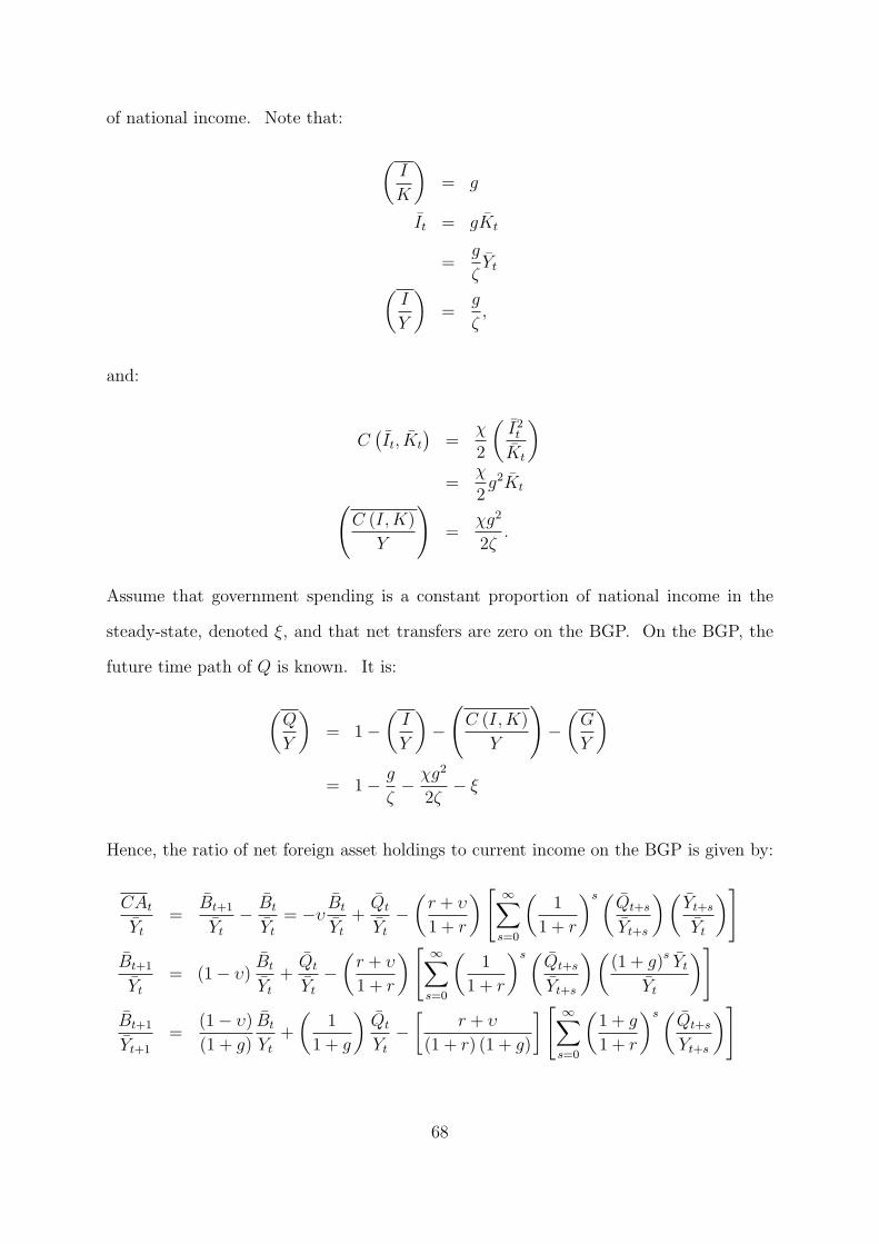
of national income. Note that:
(
I
K
)
= g
It = gKt
=g
ζYt
(
I
Y
)
=g
ζ,
and:
C(
It, Kt
)
=χ
2
(
I2t
Kt
)
=χ
2g2Kt
(
C (I,K)
Y
)
=χg2
2ζ.
Assume that government spending is a constant proportion of national income in the
steady-state, denoted ξ, and that net transfers are zero on the BGP. On the BGP, the
future time path of Q is known. It is:
(
Q
Y
)
= 1 −
(
I
Y
)
−
(
C (I,K)
Y
)
−
(
G
Y
)
= 1 −g
ζ−
χg2
2ζ− ξ
Hence, the ratio of net foreign asset holdings to current income on the BGP is given by:
CAt
Yt
=Bt+1
Yt
−Bt
Yt
= −υBt
Yt
+Qt
Yt
−
(
r + υ
1 + r
)
[
∞∑
s=0
(
1
1 + r
)s(Qt+s
Yt+s
)(
Yt+s
Yt
)
]
Bt+1
Yt
= (1 − υ)Bt
Yt
+Qt
Yt
−
(
r + υ
1 + r
)
[
∞∑
s=0
(
1
1 + r
)s(Qt+s
Yt+s
)(
(1 + g)sYt
Yt
)
]
Bt+1
Yt+1
=(1 − υ)
(1 + g)
Bt
Yt
+
(
1
1 + g
)
Qt
Yt
−
[
r + υ
(1 + r) (1 + g)
]
[
∞∑
s=0
(
1 + g
1 + r
)s(Qt+s
Yt+s
)
]
68

(
B
Y
)
=(1 − υ)
(1 + g)
(
B
Y
)
+
(
1
1 + g
)(
Q
Y
)
−
[
r + υ
(1 + r) (1 + g)
](
Q
Y
)
[
∞∑
s=0
(
1 + g
1 + r
)s]
.
For the ratio of net foreign assets to output on the BGP to be bounded, it is necessary
that g < r (else the infinite series in the above expression will not converge). The BGP
ratio of net foreign assets to output is then determined by:
[
1 −(1 − υ)
(1 + g)
](
B
Y
)
=
(
1
1 + g
)(
Q
Y
)
−
[
r + υ
(1 + r) (1 + g)
](
1 + r
r − g
)(
Q
Y
)
[
g + υ
1 + g
](
B
Y
)
=
(
1
1 + g
)(
Q
Y
)
−
[
r + υ
1 + g
](
1
r − g
)(
Q
Y
)
(g + υ)
(
B
Y
)
=
[
1 −
(
r + υ
r − g
)](
Q
Y
)
(g + υ)
(
B
Y
)
=
[
−g − υ
r − g
](
Q
Y
)
(
B
Y
)
=
[
−1
r − g
](
Q
Y
)
Notice that this implies that(
CAY
)
= g(
BY
)
on the BGP (the ratio is stationary), while
CA on the BGP is growing (the level is nonstationary).6
A.1.2 Response to A Physical Capital Shock
What is the response of the current account and other measures at the time of an unan-
ticipated negative physical capital shock in the perfect foresight model? For now, assume
that ∂T∂K
= ∂G∂K
= 0 at all times. The components of the current account response are
given by:
∂CAt
∂Kt
= −υ∂Bt
∂Kt
+∂Qt
∂Kt
−
(
r + υ
1 + r
)
[
∞∑
s=0
(
1
1 + r
)s∂Qt+s
∂Kt
]
6The derivation is:(
CA
Y
)
=
(
B
Y
)
(1 + g) −
(
B
Y
)
= g
(
B
Y
)
.
69

∂Bt
∂Kt
= 0, since Bt is chosen in the prior period.
∂Qt
∂Kt
=∂Yt
∂Kt
− (1 + CI (It, Kt))∂It
∂Kt
− CK (It, Kt)
∂Yt
∂Kt
= αYt
Kt
= αA1−αt Kα−1
t > 0
1 + χIt
Kt
= qt = e2
(
Yt
Kt
− ζ
)
+ q > 0, for Zt =
(
Yt
Kt
− ζ
)
> −
(
1 + χg
e2
)
. ⇒
∂It
∂Kt
=∂[
e2
χ(Yt − ζKt) + gKt
]
∂Kt
=e2
χ
(
αYt
Kt
− ζ
)
+ g < 0, for Zt <(1 − α)
αζ −
χg
αe2
.
CK (It, Kt) = −χ
2
(
It
Kt
)2
= −χ
2
(
qt − 1
χ
)2
= −
(
e2
(
Yt
Kt− ζ)
+ χg)2
2χ< 0 ⇒
∂Qt
∂Kt
= αYt
Kt
−
[
e2
(
Yt
Kt
− ζ
)
+ q
] [
e2
χ
(
αYt
Kt
− ζ
)
+ g
]
+
(
e2
(
Yt
Kt− ζ)
+ χg)2
2χ> 0.
∂Qt+s
∂Kt
=∂Yt+s
∂Kt
−
(
1 + χIt+s
Kt+s
)
∂It+s
∂Kt
+χ
2
(
It+s
Kt+s
)2∂Kt+s
∂Kt
∂Yt+s
∂Kt
= αA1−αt+s Kα−1
t+s
∂Kt+s
∂Kt
= αYt+s
Kt+s
∂Kt+s
∂Kt
∂It+s
∂Kt
=∂[
e2
χ(Yt+s − ζKt+s) + gKt+s
]
∂Kt
=
e2
χ
(
αYt+s
Kt+s
− ζ
)
+ g
∂Kt+s
∂Kt
< 0,
for Zt restricted as above.
Kt+s = Kt +s−1∑
j=0
It+j
∂Kt+s
∂Kt
= 1 +s−1∑
j=0
∂It+j
∂Kt
A recursion can then be set up by noting that:
∂Kt+1
∂Kt
= 1 +∂It
∂Kt
= 1 +
e2
χ
(
αYt
Kt
− ζ
)
+ g
> 0, given that Zt >(1 − α)
αζ −
(χ + χg)
αe2
.
∂It+1
∂Kt
=
e2
χ
(
αYt+1
Kt+1
− ζ
)
+ g
∂Kt+1
∂Kt
=
e2
χ
(
αYt+1
Kt+1
− ζ
)
+ g
[
1 +
e2
χ
(
αYt
Kt
− ζ
)
+ g
]
< 0
∂Kt+2
∂Kt
= 1 +∂It
∂Kt
+∂It+1
∂Kt
70

= 1 +
e2
χ
(
αYt
Kt
− ζ
)
+ g
+
e2
χ
(
αYt+1
Kt+1
− ζ
)
+ g
·
[
1 +
e2
χ
(
αYt
Kt
− ζ
)
+ g
]
=
[
1 +
e2
χ
(
αYt
Kt
− ζ
)
+ g
][
1 +
e2
χ
(
αYt+1
Kt+1
− ζ
)
+ g
]
> 0
∂It+2
∂Kt
=
e2
χ
(
αYt+2
Kt+2
− ζ
)
+ g
∂Kt+2
∂Kt
=
e2
χ
(
αYt+2
Kt+2
− ζ
)
+ g
[
1 +
e2
χ
(
αYt
Kt
− ζ
)
+ g
]
·
[
1 +
e2
χ
(
αYt+1
Kt+1
− ζ
)
+ g
]
< 0
∂Kt+3
∂Kt
= 1 +∂It
∂Kt
+∂It+1
∂Kt
+∂It+2
∂Kt
=
[
1 +
e2
χ
(
αYt
Kt
− ζ
)
+ g
][
1 +
e2
χ
(
αYt+1
Kt+1
− ζ
)
+ g
]
+
e2
χ
(
αYt+2
Kt+2
− ζ
)
+ g
[
1 +
e2
χ
(
αYt
Kt
− ζ
)
+ g
]
·
[
1 +
e2
χ
(
αYt+1
Kt+1
− ζ
)
+ g
]
=
[
1 +
e2
χ
(
αYt
Kt
− ζ
)
+ g
][
1 +
e2
χ
(
αYt+1
Kt+1
− ζ
)
+ g
]
·
[
1 +
e2
χ
(
αYt+2
Kt+2
− ζ
)
+ g
]
> 0
∂Kt+s
∂Kt
=s−1∏
i=0
[
1 +
e2
χ
(
αYt+i
Kt+i
− ζ
)
+ g
]
> 0
∂It+s
∂Kt
=
e2
χ
(
αYt+s
Kt+s
− ζ
)
+ g
s−1∏
i=0
[
1 +
e2
χ
(
αYt+i
Kt+i
− ζ
)
+ g
]
< 0
The model then means that:
∂Qt+s
∂Kt
=∂Yt+s
∂Kt
− (1 + CI (It+s, Kt+s))∂It+s
∂Kt
− CK (It+s, Kt+s)∂Kt+s
∂Kt
= αYt+s
Kt+s
∂Kt+s
∂Kt
−
(
1 + xIt+s
Kt+s
)
e2
χ
(
αYt+s
Kt+s
− ζ
)
+ g
∂Kt+s
∂Kt
+ χ
(
It
Kt
)2∂Kt+s
∂Kt
=
αYt+s
Kt+s
−
(
1 + xIt+s
Kt+s
)
e2
χ
(
αYt+s
Kt+s
− ζ
)
+ g
+ χ
(
It+s
Kt+s
)2
∂Kt+s
∂Kt
=
αYt+s
Kt+s
−
(
1 + xIt+s
Kt+s
)
e2
χ
(
αYt+s
Kt+s
− ζ
)
+ g
+ χ
(
It+s
Kt+s
)2
71

·
s−1∏
i=0
[
1 +
e2
χ
(
αYt+i
Kt+i
− ζ
)
+ g
]
=
αYt+s
Kt+s
− qt+s
e2
χ
(
αYt+s
Kt+s
− ζ
)
+ g
+ χ
(
qt+s − 1
χ
)2
·
s−1∏
i=0
[
1 +
e2
χ
(
αYt+i
Kt+i
− ζ
)
+ g
]
> 0
The current account response is then:
∂CAt+s
∂Kt
=∂Qt+s
∂Kt
−
(
r + υ
1 + r
)
[
∞∑
w=s
(
1
1 + r
)w−s∂Qt+w
∂Kt
]
=
αYt+s
Kt+s
− qt+s
e2
χ
(
αYt+s
Kt+s
− ζ
)
+ g
+ χ
(
qt+s − 1
χ
)2
−
(
r + υ
1 + r
)
[
∞∑
w=s
(
1
1 + r
)w−s
αYt+w
Kt+w
− qt+w
e2
χ
(
αYt+w
Kt+w
− ζ
)
+ g
+χ
(
qt+w − 1
χ
)2
w−1∏
i=0
[
1 +
e2
χ
(
αYt+i
Kt+i
− ζ
)
+ g
]
]
.
Recall that:
qt+s − q(
Yt+s
Kt+s
)
− ζ
=
e2
[(
Yt+s
Kt+s
)
− ζ]
λs2
[(
YK
)
t− ζ]
,
along the linearized saddle path. By substituting the saddle path equations into the
current account response, an explicit expression for the current account response can
be found. The response is a function of the initial size of the physical capital shock
(captured by(
YK− ζ)
) and how far in the past the shock was (captured by s).
No Physical Capital Adjustment Costs Case Such a complicated current account
response is difficult to interpret without simulating. In order to gain a better intuitive
understanding of the dynamics, I simplify the model, by imposing the restriction that
there are no physical capital adjustment costs (χ = 0). The underlying pattern of
dynamics should be roughly similar to that of the more general model, but with responses
occurring much quicker since there is no sluggishness in the model. In the absence of
72

capital adjustment costs, the capital Euler equation implies:
As+1F′ (Ks + Is) = r.
The capital stock would jump to its BGP immediately after a physical capital shock.
In response to an unforeseen negative physical capital shock, investment will thus be
temporarily greater than its BGP level. Assuming that ∂N∂K
= ∂G∂K
= 0, the model’s
dynamic response to a physical capital shock is described by:
∂It
∂Kt
= −1 < 0, by the implicit function theorem.
∂It+s
∂Kt
= 0, for s > 0.
∂Kt
∂Kt
= 1 > 0.
∂Kt+s
∂Kt
=∂(
Kt +∑s−1
j=0 It+j
)
∂Kt
= 1 − 1 = 0, for s > 0.
∂Yt+s
∂Kt
= αYt+s
Kt+s
∂Kt+s
∂Kt
=
α Yt
Kt> 0, for s = 0.
0, for s > 0.
∂Wt+s
∂Kt
= (1 + r)∂Bt+s
∂Kt
+∞∑
i=0
(
1
1 + r
)i [∂Yt+s+i
∂Kt
−∂It+s+i
∂Kt
]
=
α Yt
Kt+ 1, for s = 0.
(1 + r) ∂Bt+s
∂Kt, for s > 0.
∂Ct+s
∂Kt
=
(
r + υ
1 + r
)
∂Wt+s
∂Kt
=
(
r+υ1+r
)
(
α Yt
Kt+ 1)
, for s = 0.
(r + υ) ∂Bt+s
∂Kt, for s > 0.
∂Qt+s
∂Kt
=∂Yt+s
∂Kt
−∂It+s
∂Kt
=
α Yt
Kt+ 1, for s = 0.
0, for s > 0.
73

∂CAt+s
∂Kt
=∂Bt+s+1
∂Kt
−∂Bt+s
∂Kt
= −υ∂Bt+s
∂Kt
+∂Qt+s
∂Kt
−
(
r + υ
1 + r
)
[
∞∑
i=0
(
1
1 + r
)i∂Qt+s+i
∂Kt
]
⇒
∂CAt
∂Kt
=∂Bt+1
∂Kt
=
(
1 −r + υ
1 + r
)(
αYt
Kt
+ 1
)
> 0, since υ ∈ (−r, 1) .
∂CAt+s
∂Kt
= −υ∂Bt+s
∂Kt
=∂Bt+s+1
∂Kt
−∂Bt+s
∂Kt
⇒∂Bt+s+1
∂Kt
= (1 − υ)∂Bt+s
∂Kt
, for s > 0.
∂Bt+s
∂Kt
= (1 − υ)s−1 ∂Bt+1
∂Kt
⇒
∂CAt+s
∂Kt
= −υ (1 − υ)s−1 ∂Bt+1
∂Kt
> 0, if υ ∈ (−r, 0) .
= 0, if υ = 0.
< 0, if υ ∈ (0, 1) .
Since υ ∈ (−r, 1), the recursive formula for net foreign assets reveals that future net
foreign asset changes are of the same sign as the initial net foreign asset change, but
shrinking in magnitude. Hence, the current account response for s > 0 is given by:
∂CAt+s
∂Kt
= −υ (1 − υ)s ∂Bt+1
∂Kt
< 0, for s > 0 and υ ∈ (0, 1) .
The current account has an S-shaped response if the country is impatient, with the initial
sign of the response identical to the sign of the capital shock.
Stationary transformations of the above variables behave in a qualitatively similar
fashion to their levels. The contemporaneous response of the ratio of the current account
to national income is then:
∂(
CAt
Yt
)
∂Kt
=∂CAt
∂Kt
Yt
−CAt
Yt
∂Yt
∂Kt
Yt
=
(
1 −r + υ
1 + r
)(
α1
Kt
+1
Yt
)
−CAt
Yt
[
α1
Kt
]
=
(
1 −r + υ
1 + r−
CAt
Yt
)[
α1
Kt
]
+
(
1 −r + υ
1 + r
)(
1
Yt
)
> 0,
sinceCAt
Yt
<
(
1 −r + υ
1 + r
)
.
74
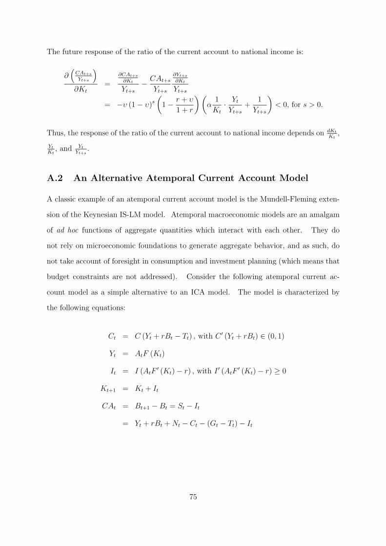
The future response of the ratio of the current account to national income is:
∂(
CAt+s
Yt+s
)
∂Kt
=
∂CAt+s
∂Kt
Yt+s
−CAt+s
Yt+s
∂Yt+s
∂Kt
Yt+s
= −υ (1 − υ)s
(
1 −r + υ
1 + r
)(
α1
Kt
·Yt
Yt+s
+1
Yt+s
)
< 0, for s > 0.
Thus, the response of the ratio of the current account to national income depends on dKt
Kt,
Yt
Kt, and Yt
Yt+s.
A.2 An Alternative Atemporal Current Account Model
A classic example of an atemporal current account model is the Mundell-Fleming exten-
sion of the Keynesian IS-LM model. Atemporal macroeconomic models are an amalgam
of ad hoc functions of aggregate quantities which interact with each other. They do
not rely on microeconomic foundations to generate aggregate behavior, and as such, do
not take account of foresight in consumption and investment planning (which means that
budget constraints are not addressed). Consider the following atemporal current ac-
count model as a simple alternative to an ICA model. The model is characterized by
the following equations:
Ct = C (Yt + rBt − Tt) , with C ′ (Yt + rBt) ∈ (0, 1)
Yt = AtF (Kt)
It = I (AtF′ (Kt) − r) , with I ′ (AtF
′ (Kt) − r) ≥ 0
Kt+1 = Kt + It
CAt = Bt+1 − Bt = St − It
= Yt + rBt + Nt − Ct − (Gt − Tt) − It
75

Aggregate consumption, denoted by C, is thus a standard Keynesian consumption func-
tion, depending upon disposable income.7 Aggregate output Y is a function of Hicks-
neutral total factor productivity A and the physical capital stock K. Here, F (·) is a
standard concave production function, with FK > 0 and FKK < 0. Aggregate invest-
ment I is an increasing function of the difference between the current marginal product
of capital and the world real interest rate r. B is net foreign asset holdings, yielding a
risk-free rate of return of r, which is the constant world real interest rate.8 G, T , and N
are respectively, government spending, lump-sum taxes, and net transfers from abroad.
As usual, the current account is defined to be the difference in net foreign assets, or the
difference between domestic saving and investment.
Further, suppose that:
dKt+1
dKt
= 1 +∂It
∂Kt
= 1 + I ′ (AtF′ (Kt) − r) AtF
′′ (Kt) > 0, by assumption.
This implies that dKt+1
dKt∈ (0, 1). There is some persistence in the capital stock; capital
adjusts sluggishly.
The model then has a transparent recursive structure. Define σt = (1 − C ′ (Yt + rBt)).
Ignoring changes in government spending, taxes, and net transfers from abroad, the
contemporaneous and future current account responses are:9
∂CAt
∂Kt
= [1 − C ′ (Yt + rBt)] AtF′ (Kt) − I ′ (AtF
′ (Kt) − r) AtF′′ (Kt)
= [1 − C ′t] AtF
′t − I ′
tAtF′′t ≡ Ωt =
∂Bt+1
∂Kt
> 0
∂CAt+1
∂Kt
=∂St+1
∂Kt
−∂It+1
∂Kt
7Consumers are assumed to hold net foreign assets, B.8Recall that the timing convention for net foreign assets B is such that Bt is determined at time t−1.
Thus, Bt is unaffected by events at time t.9Here, I will suppress the function arguments as they are understood, while maintaining the time
subscripts.
76

=[
1 − C ′t+1
]
At+1F′t+1
dKt+1
dKt
+[
1 − C ′t+1
]
r∂Bt+1
∂Kt
− I ′t+1At+1F
′′t+1
dKt+1
dKt
> 0
=[
1 − C ′t+1
]
At+1F′t+1 − I ′
t+1At+1F′′t+1
dKt+1
dKt
+[
1 − C ′t+1
]
rΩt
= Ωt+1dKt+1
dKt
+ σt+1r∂Bt+1
∂Kt
> 0
⇒∂Bt+2
∂Kt
=∂CAt+1
∂Kt
+∂Bt+1
∂Kt
> 0
∂CAt+2
∂Kt
=∂St+2
∂Kt
−∂It+2
∂Kt
=[
1 − C ′t+2
]
At+2F′t+2
dKt+2
dKt+1
dKt+1
dKt
+[
1 − C ′t+2
]
r∂Bt+2
∂Kt
−I ′t+2At+2F
′′t+2
dKt+2
dKt+1
dKt+1
dKt
= Ωt+2dKt+2
dKt+1
dKt+1
dKt
+ σt+2r∂Bt+2
∂Kt
> 0
⇒∂Bt+3
∂Kt
=∂CAt+2
∂Kt
+∂Bt+2
∂Kt
> 0
∂CAt+3
∂Kt
= Ωt+3dKt+3
dKt+2
dKt+2
dKt+1
dKt+1
dKt
+ σt+3r∂Bt+3
∂Kt
> 0
∂CAt+s
∂Kt
= Ωt+s
s∏
i=1
dKt+i
dKt+i−1
+ σt+sr∂Bt+s
∂Kt
> 0
⇒∂Bt+s+1
∂Kt
= Ωt+s
s∏
i=1
dKt+i
dKt+i−1
+ (1 + σt+sr)∂Bt+s
∂Kt
The first term of the period (t + s) current account response goes to zero, as s → ∞.10
Consider the expression for the change in net foreign assets as s → ∞. A bound on the
limiting change in net foreign assets can be found by setting σ = 1 (this is the upper
bound of σ), and solving the resulting limiting linear difference equation.11 In this case,
10For the response of the future capital stock to changes in the current capital stock to diminish overtime, it is necessary that:
dKt+2
dKt+1
dKt+1
dKt
−dKt+1
dKt
< 0
(
dKt+2
dKt+1
− 1
)
dKt+1
dKt
< 0
dKt+2
dKt+1
< 1.
This is true by assumption. The derivative of the investment function and the second derivative of theproduction function must both be finite, and furthermore, cannot grow in magnitude overly quickly (elsethey would dominate the declining capital stock response).
11L denotes the standard lag operator.
77
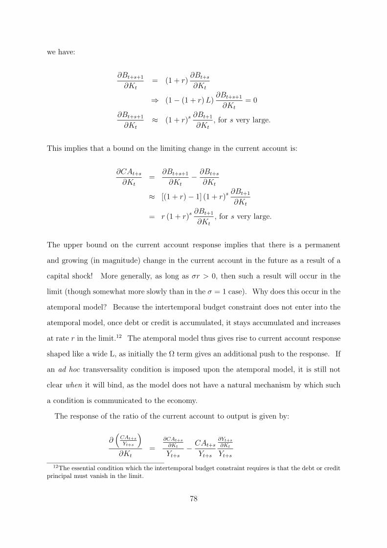
we have:
∂Bt+s+1
∂Kt
= (1 + r)∂Bt+s
∂Kt
⇒ (1 − (1 + r) L)∂Bt+s+1
∂Kt
= 0
∂Bt+s+1
∂Kt
≈ (1 + r)s ∂Bt+1
∂Kt
, for s very large.
This implies that a bound on the limiting change in the current account is:
∂CAt+s
∂Kt
=∂Bt+s+1
∂Kt
−∂Bt+s
∂Kt
≈ [(1 + r) − 1] (1 + r)s ∂Bt+1
∂Kt
= r (1 + r)s ∂Bt+1
∂Kt
, for s very large.
The upper bound on the current account response implies that there is a permanent
and growing (in magnitude) change in the current account in the future as a result of a
capital shock! More generally, as long as σr > 0, then such a result will occur in the
limit (though somewhat more slowly than in the σ = 1 case). Why does this occur in the
atemporal model? Because the intertemporal budget constraint does not enter into the
atemporal model, once debt or credit is accumulated, it stays accumulated and increases
at rate r in the limit.12 The atemporal model thus gives rise to current account response
shaped like a wide L, as initially the Ω term gives an additional push to the response. If
an ad hoc transversality condition is imposed upon the atemporal model, it is still not
clear when it will bind, as the model does not have a natural mechanism by which such
a condition is communicated to the economy.
The response of the ratio of the current account to output is given by:
∂(
CAt+s
Yt+s
)
∂Kt
=
∂CAt+s
∂Kt
Yt+s
−CAt+s
Yt+s
∂Yt+s
∂Kt
Yt+s
12The essential condition which the intertemporal budget constraint requires is that the debt or creditprincipal must vanish in the limit.
78

=
Ωt+s
∏s
i=1dKt+i
dKt+i−1+ σt+sr
∂Bt+s
∂Kt
Yt+s
−CAt+s
Yt+s
At+sF′ (Kt+s)
∏s
i=1dKt+i
dKt+i−1
Yt+s
The first term here is positive, while the sign of the second term depends upon the sign
of CAt+s
Yt+s. If CAt+s
Yt+s< 0, then the future response of the current account over output
is unambiguously positive. In the case where CAt+s
Yt+s> 0, a sufficient condition for the
future response to be positive is that CAt+s
Yt+s<
Ωt+s
At+sF ′
t+s
+σt+sr
∂Bt+s
∂Kt
At+sF ′
t+s
s
i=1
dKt+i
dKt+i−1
, which occurs
almost surely in the limit as the denominator on the second term goes to zero. Thus,
the response of the current account to output ratio is also L-shaped.
79
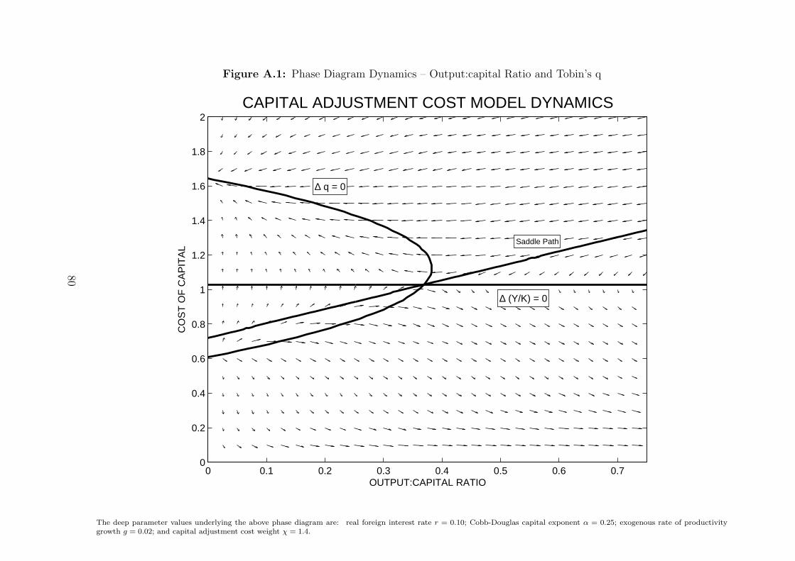
Figure A.1: Phase Diagram Dynamics – Output:capital Ratio and Tobin’s q
0 0.1 0.2 0.3 0.4 0.5 0.6 0.70
0.2
0.4
0.6
0.8
1
1.2
1.4
1.6
1.8
2
OUTPUT:CAPITAL RATIO
CO
ST
OF
CA
PIT
AL
CAPITAL ADJUSTMENT COST MODEL DYNAMICS
∆ q = 0
∆ (Y/K) = 0
Saddle Path
The deep parameter values underlying the above phase diagram are: real foreign interest rate r = 0.10; Cobb-Douglas capital exponent α = 0.25; exogenous rate of productivitygrowth g = 0.02; and capital adjustment cost weight χ = 1.4.
80