The role of seasonal timing and ... - Community Ecology

REV IEW AND

SYNTHES IS The role of seasonal timing and phenological shifts for species

coexistence

Volker H. W. Rudolf

BioSciences Program in Ecology &

Evolutionary Biology Rice University

Houston, TX, USA

Correspondence: E-mail:

[email protected]

Abstract

Shifts in the phenologies of coexistence species are altering the temporal structure of natural com-munities worldwide. However, predicting how these changes affect the structure and long-termdynamics of natural communities is challenging because phenology and coexistence theory havelargely proceeded independently. Here, I propose a conceptual framework that incorporates sea-sonal timing of species interactions into a well-studied competition model to examine how changesin phenologies influence long-term dynamics of natural communities. Using this framework Idemonstrate that persistence and coexistence conditions strongly depend on the difference in spe-cies’ mean phenologies and how this difference varies across years. Consequently, shifts in meanand interannual variation in relative phenologies of species can fundamentally alter the outcomeof interactions and the potential for persistence and coexistence of competing species. Theseeffects can be predicted by how per-capita effects scale with differences in species’ phenologies. Ioutline how this approach can be parameterized with empirical systems and discuss how it fitswithin the context of current coexistence theory. Overall, this synthesis reveals that phenology ofspecies interactions can play a crucial yet currently understudied role in driving coexistence andbiodiversity patterns in natural systems and determine how species will respond to future climatechange.

Keywords

Climate change, coexistence, community dynamics, competition, mismatch, phenology, priorityeffect, seasonal variation.

Ecology Letters (2019) 22: 1324–1338

INTRODUCTION

Ecological communities are shaped by two fundamental axes:space and time. Although ecologists have long recognized thatspecies interactions are constantly varying over time (Elton1927; Hutchinson 1961), the traditional approach to commu-nity ecology has largely focused on space and taken a fairlytemporally static view of species interactions (Wolkovich et al.2014). For instance, classical Lotka-Voltera type competition,predation, and food web models allow number of individualsto vary, but traits such as per-capita interaction coefficientsare typically assumed to be constant (i.e., time invariant). Thissimplification clearly contrasts with nature where life historytraits and species interactions are highly seasonal and con-stantly change over time with changes in phenologies andenvironmental constraints (Dunbar et al. 2009; Yang &Rudolf 2010; Diez et al. 2012; Wolkovich et al. 2014). Fur-thermore, climate change is constantly modifying the temporalstructure of species interactions (Nakazawa & Doi 2012;Wolkovich et al. 2014; Kharouba et al. 2018), which chal-lenges many of the core assumptions of fundamental conceptsand models in ecology. Indeed, accounting for temporal fluc-tuations can be essential to predict species coexistence andcommunity structure (Chesson 2000; Adler et al. 2006; Angertet al. 2009; Usinowicz et al. 2012). Consequently, there is apressing need to build a temporally explicit framework that

explicitly accounts for the seasonal structure of species inter-actions to predict dynamics and structure of natural commu-nities in a changing world.Most species interactions are highly seasonally structured:

the phenology of a species determines when and at what stageor size individuals interact with other members of the commu-nity (Yang & Rudolf 2010). For instance, a tadpole thathatches first within a growing season will initially face smallerand fewer interspecific competitors than a tadpole thathatches mid-season. Thus, the various phenologies of con-stituent species within a community define a ‘timetable’ thatdescribes the days when interactions are initiated and whenthey end for all species interactions within a communitywithin a given year. However, the seasonal timing of interac-tions is not fixed, but rather naturally varies across years (e.g.,due to fluctuations in local weather conditions) (Singer &Parmesan 2011; Diez et al. 2012). Furthermore, climatechange is altering the timing and temporal overlap of interact-ing species worldwide, leading to non-stationary (directional)changes in timing of interactions in aquatic and terrestrial sys-tems across a wide range of taxa and types of interactions(Walther et al. 2002; Parmesan & Yohe 2003; Parmesan 2006;Durant et al. 2007; Thackeray et al. 2016; Cohen et al. 2018).Despite recent advances emphasizing the importance of timingfor key coexistence mechanisms (Godoy & Levine 2014), itremains unclear how changes in the timing of species

© 2019 John Wiley & Sons Ltd/CNRS

Ecology Letters, (2019) 22: 1324–1338 doi: 10.1111/ele.13277

mailto:

interactions influence the long-term dynamic and structure ofcommunities, species coexistence, and maintenance of biodi-versity (Forrest & Miller-Rushing 2010; Wolkovich et al.2014; Visser 2016).The importance of the temporal co-ordination of phenolo-

gies for species interactions and community dynamics can beunderstood in the framework of seasonal community assem-bly. Each year, many temporary communities are largelyreassembled anew: the appearance of new offspring in sea-sonal habitats represents annual cycles of habitat re-coloniza-tion, followed by periods where individuals grow and interactwith each other. For example, many pond assemblages arereconstituted each year as terrestrial adults (e.g., insects,amphibians) return to ponds to breed, and aquatic stages oftheir life cycles interact during their ontogeny. Similar annualrecolonization events occur in annual plant communitieswhere the timing of germination from a seedbank determinesthe ‘arrival’ of individuals in the community, and many othertemporary systems. The relative phenologies (e.g., timing ofbreeding, hatching, emergence from dormancy or germina-tion) of species determine in what sequence species’ offspringarrive in the community in a given year (e.g. Godoy & Levine2014). Furthermore, phenologies vary naturally across yearsand sites leading to interannual variation in relative timing ofspecies interactions (Høye & Forchhammer 2008; Thackerayet al. 2016; Rudolf 2018) and this variation is likely toincrease with climate change (Pearse et al. 2017). Recent stud-ies indicate that even small changes in the timing of speciesinteractions can result in substantial changes in the outcomeof species interactions (Stier et al. 2013; Godoy & Levine2014; Rasmussen et al. 2014; Cleland et al. 2015; Young et al.2015; Murillo-Rinc�on et al. 2017; Rudolf 2018; Alexander andLevine, 2019). This implies that per-capita interactionstrengths are typically not constant, but instead naturallychange over time with shifts in the relative phenologies ofinteracting species within and across years (e.g., Fig. 1). It isunclear, however, when we can safely ignore this variation(e.g., as in classical Lotka-Volterra type models and foodwebs) and when we need to account for the seasonal timingof interactions to avoid erroneous conclusions and predic-tions. Temporal variation in environmental conditions thatinfluence the fitness of competing species (e.g., temporal stor-age effect) can play a key role in determining coexistence pat-terns (Chesson 2000; Barab�as et al. 2018). Variation in thetemporal co-ordination (phenology) of species interactionscould be similarly important and act as a ubiquitous, but cur-rently overlooked driver of species coexistence and biodiver-sity patterns. However, we still lack a general theoreticalframework that incorporates these empirical patterns intoexisting community models to examine and predict the long-term effects of this temporal co-ordination in interactions.To help fill this conceptual gap I propose a general theoretical

framework that links shifts in relative seasonal timing of interac-tions (phenologies) and interannual variation in relative phenolo-gies to well-studied competition models. Specifically I focus on awell-studied competition system to study when and how differentaspects (i.e., mean and variance) of temporal changes in the tim-ing of species interactions are expected to alter persistence andextinction rates of competing species and coexistence conditions.

Integrating seasonal timing and phenological shifts into community

models

To examine the consequences of changes in the mean andvariation of species’ phenologies across years we can incorpo-rate shifts in the timing of species interactions into classicaltime discrete community models in two steps. First, wedescribe population dynamics and species interactions withina year (i.e., seasonal) by modelling per-capita interactionstrength as a function of relative phenologies (arrival times) ofinteracting species (Fig. 1). Second, populations are projectedfrom one year to the next based on their specific demographicrates (e.g., adult longevity, fecundity, etc.). This approachallows one to systematically manipulate mean and variationof relative timing of species phenologies across years andexamine the long-term consequences for community dynam-ics.Here, I apply this approach to a well-studied two-species

Beverton-Holt type competition models (Beverton & Holt1957). The model describes the change in the population size(Ni) of competing species i and j between two consecutiveyears (t ? t+1) as:

Ni;tþ1 ¼ kiNi;t

1þ aiikiNi;t þ fij Dpij;t� �

kjNj;t

� �þ siNi;t:

Nj;tþ1 ¼ kjNj;t

1þ ajjkjNj;t þ fji Dpji;t� �

kiNi;t

� �þ sjNj;t:

with si indicating the proportion of adults that survive to thenext year. The number of new adults is given by the maxi-mum recruitment rate ki in the absence of competition (theproduct of fecundity of a species and probability of survivingto adult stage in absence of competition) which declines withthe sum of intraspecific (aiikiNi;t) and interspecific(fij D pji;t

� �kiNi;t) competition. Here, I adjusted the model to

reflect common conditions in natural temporary/seasonalcommunities in nature, where density-dependent regulationfrom intra- and interspecific competition is largely restrictedto offspring (e.g., tadpoles or dragonfly larva in temporaryponds). Thus, the density of the competitor is given by thenumber of new offspring at the beginning of a year: kjNj;t.However, the model can easily be modified to represent othersystems (e.g. annual plant communities Godoy & Levine2014).One key innovation here is that the per-capita effect of

interacting species, fij D pij;t� �

; is a function of relative differ-ences in timing of species’ phenologies ðD pij;tÞ (e.g., the num-ber of days between emergence of species i and j within agiven year t). Thus, interspecific interaction coefficients arenot constant, ‘intrinsic’ traits of species in a given environ-ment as in classical community models, but instead they aretemporally explicit and allowed to vary across years. Thismodification of interspecific interactions accounts for the factthat changes in relative phenologies typically lead to concur-rent changes in per-capita strength of competitive effects innatural systems, without the need to identify the specificunderlying mechanisms. Note that the same type of mod-elling approach can easily be extended to other types of


Review and Synthesis Phenology timing and species coexistence 1325

interactions (e.g., predator-prey, mutualistic interactions, par-asitism/herbivory, etc.) and to include intraspecific variationin phenology (e.g. Nakazawa & Doi 2012; Revilla et al.2014).Another advantage of this model formulation is that we can

easily parameterize the competition–phenology functions fjfrom experiments (Rudolf 2018), which allows us to simulatecompetitive dynamics for biological realistic conditions and toempirically tests predictions in the future. Figure 1 gives aworked example of how this can be done in a few steps. Fur-thermore, given a stationary system (i.e., no changes in meanphenologies over time) and no interannual variation in rela-tive phenologies, the difference in arrival time is always thesame. In this scenario we can substitute the competition func-tion with a constant: fij D pij;t

� � ¼ aij, and the model simplifiesto a classical competition model (Beverton & Holt 1957; Les-lie & Gower 1958) without seasonal dynamics for which theinvasion and coexistence conditions are well-understood ana-lytically (Cushing et al. 2004).Theoretically, a variety of relationships of the competition–

phenology function fijðD pij;tÞ are possible, but biological sys-tems generally fall in two broad categories (Wilbur & Alford1985; Cleland et al. 2015; Clay et al. 2019): (1) Early arriver

advantage, where negative effects of interspecific competitionon a given species declines the earlier it arrives before others,and (2) late arriver advantage, where negative effects of inter-specific competition on a species decrease when it arrives laterthan its competitors. The effect of shifts in phenologiesdepends on whether interacting species fall in opposite or thesame arrival advantage category. If both species show oppo-site arrival advantage responses (i.e., one with early one withlate arrival advantage), then a shift in relative phenologies willalways either increase or decrease ~ the strength of interspeci-fic competition for both species. For instance, consider ahypothetical scenario where species i has early arriver advan-tage and species j experiences late arriver advantage. Earlierarrival of species i relative to species j will increase the earlyarriver advantage of species i and the late arriver advantageof species j, resulting in a reduction of interspecific competi-tion for both species. Of course delaying arrival of i relativeto j would result in a negative effect for both species andincrease interspecific competition. In systems where this sce-nario is true, the strength of per-capita interspecific competi-tion coefficients for both species would be positivelycorrelated across a gradient of differences in relativephenologies.

Figure 1 Example of how we can link variation in relative timing of species’ phenologies to concordant interannual variation in per-capita interaction

strength in natural systems in a few simple steps. (a) In this system, long-term observations reveal considerable interannual variation in mean differences in

first calling of Wester chorus frog, Pseudacris triseriata (PT) relative to its competitor, the Southern leopard frog, Rana sphenocephala (RS). Points indicate

mean differences averaged across eight ponds based on 15 years of daily call recordings which are expected to be correlated with differences in relative

hatching (arrival) time of tadpoles (b). Subsequent experiments which manipulated the relative hatching time of tadpoles of both species (0, 5,10,15,20 days

delay in arrival of RS) were then used to estimate how the per-capita effect of the dominant competitor (RS) affects survival of the inferior competitor

(PT). Non-linear curve fitting was then used to derive the competition arrival functions f(Dp) (blue line). (c) We can then parameterize the competition–phenology function f(Dp) with recorded annual variation in relative arrival times (a) to estimate the realized per-capita effect of R. sphenocephala (RS) on

recruitment success of P. triseriata (PT) for a given year (solid red line). For reference, solid and dashed grey lines in (c) indicate corresponding per-capita

interaction strength predicted when either assuming no difference in phenologies (Dp = 0) or based on mean differences in first calling date across

15 years, respectively. Data were extracted from (Carter et al. 2018; Rudolf 2018). Illustrations by VHWR.


1326 Rudolf Review and Synthesis

Alternatively, if both species show the same type ofresponse (e.g., both perform better when arriving before theother) a delay in relative arrival time will have opposite effectson both species. For instance, with early arriver advantage, arelative delay in arrival of species i decreases the effect of spe-cies i on j, but at the same time also increase the effect of j oni. In this scenario, interspecific per-capita interaction coeffi-cients of competing pairs of species (aij; ajiÞ are therefore nega-tively correlated along a relative arrival gradient (e.g.,Fig. 2a). However, how quickly the competitive effectincreases or declines with difference in relative arrival time(i.e., the slope of f D pij;t

� �is likely to differ across species since

species can vary in their sensitivities to shifts in relative arrivaltime (e.g. Stuble & Souza 2016; Rudolf 2018; Alexander &Levine 2019). Note that the same negative correlation andgeneral pattern hold true in systems with late arrival advan-tage for both species; in this scenario results are simply a mir-ror images (switched signs) for both species.Since early arriver advantage is by far the best documented

pattern in natural system (Fukami 2015), I largely focus onthis scenario for model analyses and numerical simulations.This type of arrival advantage (or priority effect) is well-docu-mented in plant, animal and microbial communities in varietyof terrestrial, freshwater and marine systems (Connell &Slatyer 1977; Geange & Stier 2009; Dickie et al. 2012; Her-nandez & Chalcraft 2012; Kardol et al. 2013; Rasmussenet al. 2014; Devevey et al. 2015; Stuble & Souza 2016; Rudolf

2018; Alexander and Levine, 2019). While a variety of directand indirect mechanisms can create this effect (Fukami 2015),it commonly arises in seasonal communities due to size-medi-ated priority effects (sensu Rasmussen et al. 2014), which aregenerated when interactions occur among growing individualsand per-capita interaction strength scales positively with size.It is important to keep in mind that early arriver advantagehere refers to per-capita effects and is not driven by numericaleffects (e.g., increase in population size over time) as in mostclassical priority effects models. I will return to this importantdistinction later in more detail.

DETERMINISTIC INVASION AND COEXISTENCE

CONDITIONS

We can gain a first understanding of the model dynamics andimportance of the seasonal timing (phenology) of interactionsby considering deterministic invasion and coexistence condi-tions without interannual variation in phenologies (Chesson2000; Cushing et al. 2004). In this system, the growth rate ofspecies j when rare (j ? 0) is given by:

Nj;tþ1

Nj;t¼ gjbj

1þ gi � 1½ � fjiðDpji;tÞaii

� �þ 1� bj:

with bj = 1 � sj, gi ¼ ki1�si

¼ kibi. Using some rearranging, we

can show that the growth rate of j is positive, allowing j to

αij

αji0.00

0.01

0.02

0.03

0.04

0.05

0 5 10 15 20

Difference in relative phenologies, Δ p ij

Inte

rspe

cific

com

petit

ion

coef

ficie

nts,

αij, α

ji

Sp.i+Sp.j Sp.j

Sp.i

Sp.i,Sp.j

0

5

10

15

20

0.025 0.050 0.075

Baseline per capita effect, α ij , Δp = 0

Diff

eren

ce in

rela

tive

phen

olog

ies,

Δp i

j

Figure 2 Changes in relative timing of phenologies can fundamentally alter the conditions for coexistence and create novel outcomes and states. Left panels

show a numerical example of how strength of per capita intraspecific competitive effects scale with difference in relative arrival (e.g., hatching time) in

systems with early arriver advantage for both species. Dpij indicates the difference in species phenologies (i.e., number of days species i arrives before its

competitor, species j). Here, species i is the inferior competitor when both species arrive at the same time as species j (aij;Dp¼0 = 0.5 vs. aij;Dp¼0 = 0.005).

Right panel shows how change in relative arrival time can alter conditions for persistence and coexistence of both species. The x-axis, aij;Dp¼0, indicates the

‘baseline competition coefficient’ when both species arrive at same time (Dpij = 0, see ‘Scenario 1’ for detail). In this example, increasing strength of

interspecific competition ðaijÞ can lead to a shift from stable coexistence of both species (black area) to extinction of species i (dark gray). However, a delay

in relative arrival time can allow coexistence under a larger range of aij values. Furthermore, it can result in new outcomes, including counterintuitive

extinction of species j, or alternative stable states where either species can be excluded depending on the initial conditions (white area). Outcomes are based

on relationships of ðaijÞ shown in left panel. Note that the sharp transition between system states at Dpij = 10 arises because the both competition

functions always intersect at that point (see left panel) for all aij values; if Dpij < 10 then aij [ aji, and if Dpij > 10 then aij\aji. Following empirical data

(Fig. 1), competition–phenology functions in (a) and (b) were both modelled as sigmoidal functions (see supplement for details), with A = 0.5, xmid = 10

and scali = �3, and scalj = 3. Parameters in (b) were: ajj = aii =0.025, ki = kj = 1.5, si = sj = 0.



invade from low densities in a single species system with spe-cies i present at equilibrium, if.

aiigi � 1½ � [

fjiðDpji;tÞgj � 1� � :

In other words, a species can invade and persist if the inter-specific competitor (i) has a greater net effect on itself (scaledby its life time reproduction potential: gi � 1) than the scaledcompetitive effects on the invading species for a given phenol-ogy. Using the same approach for invasion of species i, thisresult recovers the equivalent of the well-known conditions inclassical Lotka-Volterra type competition models where bothspecies can coexist if:

aiigi � 1½ � [

fjiðDpji;tÞgj � 1� � ð1Þ

and

ajjgj � 1� � [ fijðDpij;tÞ

gi � 1½ � ð2Þ

Finally, if neither species can invade when rare, the outcomedepends on the initial relative densities and relative strengthof interspecific competition leading to alternative stable states.

TIMING, COMPETITIVE DOMINANCE AND SPECIES

COEXISTENCE

Phenologies can affect species interactions and communitydynamics in two major pathways: via changes in mean timingof interactions and via changes in interannual variance (i.e.,exact seasonal timing differs across years). To isolate the indi-vidual and combined effects of both types of phenologicalchange, I divide the analysis in four different scenarios below.

Scenario 1: Shifts in mean phenologies of species interactions

The importance of changes in the relative timing of species’phenologies for coexistence conditions becomes immediatelyapparent with a bit of re-arranging of eqn 1 and eqn 2. Let ussplit the competition–phenology functions in two parts: (I) aconstant per-capita effect when both species arrive at the sametime ðaij;Dp¼0Þ, and (II) the degree to which it is modified by agiven difference in relative phenologies in a given year t(@Dpij;tÞ such that.

fij Dpij;t� � ¼ aij;Dp¼0 þ @Dpij;t ð3ÞSubstituting this formulation into the invasion and persis-

tence conditions above (eqns 1 & 2) immediately reveals asimple but non-trivial fact: we cannot predict competitivedominance and persistence of interacting species without con-sidering the timing (phenology) of interactions and how itaffects per-capita interaction strength, i.e., @Dpij;t (Fig. 2). For

instance, consider a system with early arriver advantage,where aij;Dp¼0 is too large to meet the inequality conditions in

eqn 2 when both species arrive at the same time. In this sce-nario, species i cannot invade and coexist with species j whenboth phenologies are perfectly synchronized. However, a rela-tive delay in arrival of species j would weaken its per capita

effect (i:e:@Dpij;t < 0) and thereby decrease the right hand side

of eqn 2. This would increase the invasion growth rate of spe-cies i and could ultimately allow for its persistence if the delayof j decreases the per-capita effect enough so that inequality

in eqn 2 is met, so:@Dpij;t\ajj gi�1½ �gj�1½ � � aij;Dp¼0. Thus, which species

can ultimately persist and which species will be excluded canswitch depending on the relative timing of species’ phenologies(Fig. 2). Similarly, some systems may exhibit a stable singlespecies, or coexistence equilibrium, or alternative stable statesdepending on mean relative phenologies (Fig. 2). Interestingly,these results imply that natural systems with similar speciescomposition and environmental conditions but different meanrelative phenologies can have different community dynamicsand compositions.These results also highlight an intuitive but frequently over-

looked fact in coexistence studies: species may persist andcoexist under conditions that seem implausible if we makepredictions based on classical assumption that assume equalphenologies and time-invariant (constant) interaction coeffi-cients. For instance, a species that would be considered com-petitively dominant (based on same arrival times) may beexcluded from the system if its phenology is delayed relativeto its competitor (Fig. 2). Thus, competitive dominance in sea-sonal systems should ideally be discussed in the context ofspecies’ relative timing of phenologies.The same conceptual framework outlined above also allows

us to make some predictions about how phenological shiftswill affect species interactions and community structure. If thetiming of interactions can determine their outcome, this alsoimplies that shifts in mean phenologies (e.g., due to climatechange), could alter the persistence and coexistence conditionsof natural communities. Whether a shift in relative phenolo-gies ultimately promotes or demotes coexistence of competingspecies depends on the competitive asymmetry and the direc-tion of the shift, i.e., whether it favours the competitively infe-rior species. For instance, with competitive asymmetry andearly arriver advantage (see above), a long-term phenologicalshift delaying arrival of the dominant competitor should facil-itate coexistence (Fig. 2), especially if the dominant species isless sensitive to this shift (i.e., shallower slope off Dpð Þ). In thisscenario, phenological shifts would serve as both an ‘equaliz-ing’ mechanism and potentially also as a ‘stabilizing’ mecha-nism (sensu Chesson 2000). It would be equalizing because itreduces the competitive asymmetry between species by weak-ening the effect of the dominant species and enhancing theeffect of the inferior species. It could be stabilizing if it alsoincreases the sum of both right hand sides of invasion condi-tions (eqns 1 & 2) and thus increase the invasion rate of bothspecies when rare. In contrast, if both species are competi-tively very similar, then increasing differences in phenologieswould result in competitive asymmetry and thus reduce thepotential for coexistence (reducing ‘equalizing’ mechanisms),regardless of which species is delayed.

Scenario 2: Variation in relative timing of phenologies across years

Relative timing of species’ phenologies naturally vary acrossyears, and this variation differs across systems. For instance,



a species may hatch/emerge earlier than its competitor, at thesame time, or even later depending on the year (e.g., Fig. 1).Whether and how this variation affects short- and long-termdynamics of interactions ultimately depends on whether therelationship between interaction strength and relative timingof phenologies f Dpð Þð Þ is linear or non-linear. If the competi-tion–phenology relationship is linear, then the long-term termaverage is simply the mean competition coefficient at the aver-

age difference in phenologies: fij Dpij;t� � ¼ fij Dpij;t

� �). In this

scenario variation will not alter the average per-capita interac-tion strength or equilibrium coexistence conditions of thesystem.Recent studies indicate, however, that interaction strength

can scale non-linearly with difference in relative phenologies(Rudolf 2018). Indeed, such non-linear relationships areexpected to be the norm in natural systems where interactionsoccur between growing individuals and can arise through anumber of different mechanisms (e.g., due to positive feed-backs and/or non-linear growth rates). By Jensen’s inequality(Jensen 1906), a non-linear relationship implies that interan-nual variation can modify the interaction strength (Rudolf2018). Specifically, it can either increase or decrease the aver-age interaction strength (non-linear averaging effect), depend-ing on whether the monotonic curvature of the relationshiparound the mean phenologies is convex,

@fij@Dpij

[ 0, or concave,@fij@Dpij

\0, respectively. The stronger the non-linearity, the stron-ger the effect of interannual variation becomes (e.g., Dpij = 15vs. Dpij = 5 in Fig. 3a). Interestingly, this also indicates thatpopulations with the same mean phenologies but differentlevels of interannual variation in relative phenologies will havedifferent average interaction strengths.By altering per-capita interaction strength, interannual variation

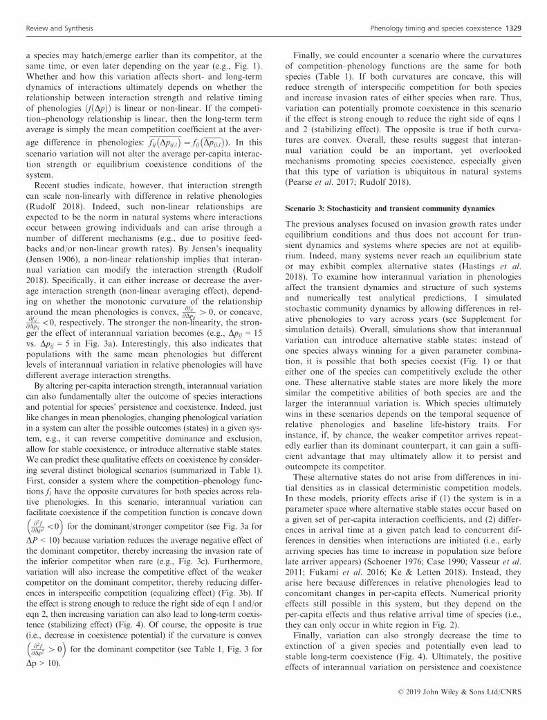
can also fundamentally alter the outcome of species interactionsand potential for species’ persistence and coexistence. Indeed, justlike changes in mean phenologies, changing phenological variationin a system can alter the possible outcomes (states) in a given sys-tem, e.g., it can reverse competitive dominance and exclusion,allow for stable coexistence, or introduce alternative stable states.We can predict these qualitative effects on coexistence by consider-ing several distinct biological scenarios (summarized in Table 1).First, consider a system where the competition–phenology func-tions fi have the opposite curvatures for both species across rela-tive phenologies. In this scenario, interannual variation canfacilitate coexistence if the competition function is concave down

@2f@Dp2 \0

� �for the dominant/stronger competitor (see Fig. 3a for

DP < 10) because variation reduces the average negative effect ofthe dominant competitor, thereby increasing the invasion rate ofthe inferior competitor when rare (e.g., Fig. 3c). Furthermore,variation will also increase the competitive effect of the weakercompetitor on the dominant competitor, thereby reducing differ-ences in interspecific competition (equalizing effect) (Fig. 3b). Ifthe effect is strong enough to reduce the right side of eqn 1 and/oreqn 2, then increasing variation can also lead to long-term coexis-tence (stabilizing effect) (Fig. 4). Of course, the opposite is true(i.e., decrease in coexistence potential) if the curvature is convex

@2f@Dp2 [ 0

� �for the dominant competitor (see Table 1, Fig. 3 for

Dp > 10).

Finally, we could encounter a scenario where the curvaturesof competition–phenology functions are the same for bothspecies (Table 1). If both curvatures are concave, this willreduce strength of interspecific competition for both speciesand increase invasion rates of either species when rare. Thus,variation can potentially promote coexistence in this scenarioif the effect is strong enough to reduce the right side of eqns 1and 2 (stabilizing effect). The opposite is true if both curva-tures are convex. Overall, these results suggest that interan-nual variation could be an important, yet overlookedmechanisms promoting species coexistence, especially giventhat this type of variation is ubiquitous in natural systems(Pearse et al. 2017; Rudolf 2018).

Scenario 3: Stochasticity and transient community dynamics

The previous analyses focused on invasion growth rates underequilibrium conditions and thus does not account for tran-sient dynamics and systems where species are not at equilib-rium. Indeed, many systems never reach an equilibrium stateor may exhibit complex alternative states (Hastings et al.2018). To examine how interannual variation in phenologiesaffect the transient dynamics and structure of such systemsand numerically test analytical predictions, I simulatedstochastic community dynamics by allowing differences in rel-ative phenologies to vary across years (see Supplement forsimulation details). Overall, simulations show that interannualvariation can introduce alternative stable states: instead ofone species always winning for a given parameter combina-tion, it is possible that both species coexist (Fig. 1) or thateither one of the species can competitively exclude the otherone. These alternative stable states are more likely the moresimilar the competitive abilities of both species are and thelarger the interannual variation is. Which species ultimatelywins in these scenarios depends on the temporal sequence ofrelative phenologies and baseline life-history traits. Forinstance, if, by chance, the weaker competitor arrives repeat-edly earlier than its dominant counterpart, it can gain a suffi-cient advantage that may ultimately allow it to persist andoutcompete its competitor.These alternative states do not arise from differences in ini-

tial densities as in classical deterministic competition models.In these models, priority effects arise if (1) the system is in aparameter space where alternative stable states occur based ona given set of per-capita interaction coefficients, and (2) differ-ences in arrival time at a given patch lead to concurrent dif-ferences in densities when interactions are initiated (i.e., earlyarriving species has time to increase in population size beforelate arriver appears) (Schoener 1976; Case 1990; Vasseur et al.2011; Fukami et al. 2016; Ke & Letten 2018). Instead, theyarise here because differences in relative phenologies lead toconcomitant changes in per-capita effects. Numerical priorityeffects still possible in this system, but they depend on theper-capita effects and thus relative arrival time of species (i.e.,they can only occur in white region in Fig. 2).Finally, variation can also strongly decrease the time to

extinction of a given species and potentially even lead tostable long-term coexistence (Fig. 4). Ultimately, the positiveeffects of interannual variation on persistence and coexistence



are contingent on the curvature of the competition functionsaround the mean (see Scenario 2, Table 1). Overall, these pat-terns are consistent with the deterministic analyses above anddriven by the same underlying mechanisms: changes in per-capita interaction strength.

Scenario 4: Non-stationary systems and the interactive effect

phenological mean and variance

So far, we have considered stationary systems where the meanand variance are constant across years. However, climatechange is altering the differences in mean phenologies of spe-cies around the world, effectively creating non-stationary sys-tems (Wolkovich et al. 2014). The model and analysesdescribed above also provide a simple and intuitive frame-work of predicting how these non-stationary changes willaffect communities. For instance, without interannual varia-tion, we can directly predict the outcome of these shifts inmean phenologies as explained in Scenario 1 (e.g., by movingalong the y axis in Fig. 2). How sensitive a system is tochanges in mean phenologies will depend on the slope of thecompetition–phenology function fðDpÞ: a shallow slopearound the current mean will result in little change in per-cap-ita effects, while a steep slope implies that even small shift in

mean phenologies can lead to dramatic changes per capitaeffects and population densities and thus is more likely toalter the persistence/coexistence potential.Most systems also exhibit natural interannual variation in

phenologies, and this variation can alter the net effect of non-stationary changes in mean phenologies, i.e., the rate at whichthe system changes. The direction and magnitude of this mod-ification effect again depends on the curvature of the competi-tion–phenology function fðDpÞ around the mean: the effect ofchanging mean phenologies will either be smaller or largerthan expected if the curve is concave or convex respectively.As a consequence, the system may change slower (or faster)than expected (e.g., Fig. 5) and this effect increases the stron-ger the curvature of the function. In many systems, mean andthe interannual variation in phenologies will both change atthe same time, and this can either enhance or delay the nega-tive (or positive) effects of shifts in the mean if the competi-tion–phenology function fðDpÞ is non-linear (see above).Overall, these results highlight the importance of interannualvariation in phenologies for mitigating the rate at which sys-tems change in response to continuous climatic change. Theyalso indicate that phenological shifts can have variable, butpredictable effects on a system that can be inferred from ageneral understanding of how per-capita interaction strength

0.00

0.01

0.02

0.03

0.04

–5 0 5 10 15 20Differences in phenologies, Δ pij

Inte

rspe

cific

com

petit

ion

coef

ficie

nts,

αij α

ji

(a) (b) (c)

–20

–10

0

10

20


Rel

ativ

e ch

ange

in c

ompe

titiv

e do

min

ace

(%)

1.0

1.1

1.2

1.3

1.4


Inva

sion

rate

Variation

0

3

6

9

12

15

18

Figure 3 Example of how interannual variation in relative timing of phenologies can change per-capita competition effects, competitive asymmetry, and

invasion rate of the inferior competitor if the competition–phenology function, fij, scales non-linear with differences in relative phenologies (e.g., hatching

time). Dpij indicates the number of days species i arrives before its competitor, species j. (a) per-capita interspecific interaction coefficient for species j on

species i (aij, solid lines) and vice versa (aji dashed lines) assuming early arriver advantage for both. (b) Proportional change in competitive dominance.

Negative values indicate reduction and positive values increase in competitive asymmetry (i.e., dominance of species j) relative to the no-variance control

scenario. (c) Invasion growth rate of inferior competitor, species i, into population of species j at equilibrium density. The invasion rate has to be > 1

(dashed black line) for successful invasion (and thus persistence) of species i. In this scenario, increasing variation can facilitate invasion and persistence of

species i with small differences in arrival time because of the concave curvature of the competition function aij in (see panel a). In all panels, different line

colours indicate average interaction strength for different levels of simulated interannual variation in arrival time around a given mean based on 9900

simulations (see Supporting Information for simulation details). Variation indicates absolute difference in relative arrival days assuming uniform

distribution with a range twice the average (no variation = 0). Parameters are: A = 0.5, xmid = 10 and scali= �3, and scalj = 3ki = kj = 1.5,

si = sj = 0, ajj = 0.04.



scales with differences in timing of relative phenologies, i.e.,the slope and curvature of the competition –phenology func-tion.

Limitations and extensions

The analysis above shows that shifts in relative timing of phe-nologies alone can change coexistence conditions by alteringper-capita interaction strength. These changes can occur evenif phenologies track optimal environmental conditions (i.e.,conditions remain mostly constant across differences in rela-tive phenologies). However, in some systems, shifts in the rela-tive timing of interactions may also be correlated with

changes in environmental conditions that influence otherdemographic parameters. For instance, a suboptimal shifts ina species phenology could expose individuals to different andpotentially detrimental environmental conditions (e.g., lowertemperatures or resource abundance), thereby reducing theirreproduction or survival (i.e., reduce k in eqn 1 & 2). In thisscenario, changes in per-capita interaction strength mediatedby shifts in relative timing of phenologies could be correlatedwith changes in other key demographic rates.We can gain a general understanding of how environmental

changes might interact with phenological shifts to influenceoutcome of species interactions using the modelling approachoutlined above. I will use k as an example here, but the same

Table 1 Effect of interannual variation on coexistence potential

Com

petit

or e

ffect

(αij)

Difference in phenologies, Δpij

Opposite curvature

Com

petit

or e

ffect

(αij)


Opposite curvature

Competitive asymmetry

Coexistence potential

Dominant: Concave upInferior: Concave down

Dominant: Concave downInferior: Concave up

Curvature of competition—phenology function f(Δp)Variance effect

on αij, αij

Com

petit

or e

ffect

( αij)


Same curvaturedominant

inferior

Com

petit

or e

ffect

(αij)


Same curvature

Dominant: Concave upInferior: Concave up

Dominant: Concave downInferior: Concave down

The curvatures of the competition–phenology function of dominant and inferior competitor around a given mean (dashed vertical line) determines whether

increasing variation in timing of interactions across years will either promote or demote the potential for coexistence. Vertical dashed lines show mean dif-

ference in phenologies across years, curves show different scenarios of competition–phenology function combinations for two competing species. Arrows

indicate qualitative, directional effects of increasing interannual variation on the strength of interspecific competitive effects (aij, aij), competitive asymmetry

(absolute differences between aij, aij) and the potential for coexistence. Colours correspond to species specific competitive effects and functions.



steps can be applied to other life-history traits. We candescribe the relationship of k and phenological shift as:ki ¼ ki þ Dki;t, where ki, where ki is the value of k for species i

when both species arrive at the same time (Dp ¼ 0Þ, and Dki;t

is the degree to which it is changed by a given shift in thephenology of species i. Note, that unlike per capita interactionstrength (e.g., aij) the change in k ði:e:;Dki;tÞ is independent ofthe phenology of other species; instead it is a function of thechange in environmental condition the focal species experi-ences. This distinction is important because it emphasizes dif-ferent underlying mechanisms that may or may not becorrelated. Substituting this expression into eqn 3, we obtainthe invasion conditions for species j:

ajjkjþDkj;t

bj� 1

h i [aij;Dp¼0 þ @Dpij;t

kiþDki;t

bi� 1

h i ð4Þ

eqn 4 indicates that changes in k mediated by an absoluteshift in species’ phenologies can alter coexistence conditionsand the result will depend on: (1) how this shift in k is corre-lated across both species ( i.e., the ratio of Dkj;t andDki;t), and(2) how this ratio in turn is correlated with shifts in interspeci-fic per capita interaction strength, @Dpij;t. The first relationshipis straight forward: if phenological shifts increase k of thecompetitor more than k of the invader, the invasion condi-tions in eqn is harder to meet, reducing the potential for theinvader to persist. The relationship between

Dkj;t

Dki;tand @Dpij;t

describes how the effect of changes in environmental condi-tions are correlated with the effect of changes in relative tim-ing of phenologies. If both are positively correlated (e.g., shiftdecreases relative k of the competitor and its competitive per-capita effect, so @Dpij;t\0 and

Dkj;t

Dki;t\1Þ, than their effects are

synergistic and shifts in the relative timing of phenologies willhave larger than expected effects solely based on shifts in per-

2

4

6

100 200 300

Time

Popu

latio

n de

nsity

Variation1

10

16

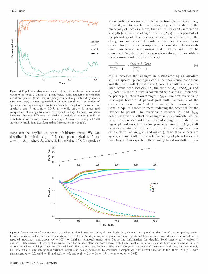
Figure 4 Population dynamics under different levels of interannual

variance in relative timing of phenologies. With negligible interannual

variation, species i (blue lines) is quickly competitively excluded by species

j (orange lines). Increasing variation reduces the time to extinction of

species i, and high enough variation allows for long-term coexistence of

species i and j. aii = ajj = 0.045, aij = 0.05, Dpij = 0; values and

competition–phenology functions correspond to Fig. 3 above. Variation

indicates absolute difference in relative arrival days assuming uniform

distribution with a range twice the average. Means are average of 9900

stochastic simulations (see Supporting Information for details).

10

15

20

25

0 100 200 300 400 500

Mea

nΔp i

j

0

2

4

6

0 100 200 300 400 500Time (Years)

Den

sity

Variation151020

Figure 5 Consequences of non-stationary, continuous shift in relative timing of phenologies (Dpij shown in top panel) on densities of two competing species.

Colours indicate level of interannual variation in arrival time (in days) around a given mean (see Fig. 4) and lines indicate mean densities smoothed across

repeated stochastic simulations (N = 100) to highlight temporal trends (see Supporting Information for details). Solid lines = early arriver i,

dashed = late arriver j. Here, shift in arrival time has smaller effect on both species with higher level of variation, slowing down and extending time to

extinction of later arriving competitor (dashed lines). E.g., populations decline > 54% in fist 100 years in absence of interannual variation, but decline only

by 14% with 20 day interannual variance which also delays extinction by centuries. Competition and arrival function follow those in Fig. 3 with

parameters: A = 0.5, xmid = 10 and scali = �3, and scalj = 3ki = kj = 1.5, si = sj = 0, ajj = 0.045.



capita interaction strength. In contrast, a negative correlationbetween

Dkj;t

Dki;tand @Dpij;t (e.g., relative increase in k of competi-

tor but decrease in its per capita competitive effect) wouldresult in antagonistic effects of both types of shift, therebyreducing or potentially reversing the effect predicted solelybased on changes in interaction strength.Unfortunately, we know little about which correlations are

more likely to occur in natural systems, and the details arelikely to be system specific. However, once the relationshipsare established for a given system, the example above demon-strates how we can easily account for such system specificdetails to predict the net effect of phenological shifts on per-sistence and coexistence in a given system. Indeed, thisapproach could be used in future studies to compare theimportance of changes in environmental conditions vs. speciesinteractions associated with phenological shifts. Regardless ofthese system specific details, the underlying mechanism remainthe same: phenological shifts can alter outcome of speciesinteractions and either promote or demote coexistence viatheir effect on competitive (as)symmetry.Finally, the model assumes that phenologies in one year are

independent of phenologies in the previous year. This is acommon assumption in phenology models (Nakazawa & Doi2012; Revilla et al. 2014) and a good first approximation formany systems where phenologies are largely driven by yearspecific seasonal cues (e.g., temperature or rain), but it maynot hold true in multivoltine systems. For instance, changes incompetition due to phenological shifts can influence develop-mental rates and thus the phenology of next life stage (Carter& Rudolf in review). However, we currently have little infor-mation on when and how the timing of phenologies is corre-lated across life-stages or generations and more data is neededbefore we can make biological realistic models to examinehow this might affect coexistence patterns.

DISCUSSION

The phenology of species interactions is increasingly recog-nized as a major force structuring natural communities, butstudies on phenologies and coexistence theory have largelyproceeded independently. The theory outlined here was specif-ically developed to help make this connection. Overall, themodel revealed that the conditions for species coexistence andpersistence could strongly be influenced by the relative timingof species’ phenologies and the outcome depends on how per-capita interaction strength scales with this timing, i.e., theshape of the competition–phenology function. As a conse-quence, any differences or shift in mean relative timing of spe-cies’ phenologies (e.g., due to climate change) has thepotential to fundamentally alter persistence and coexistenceconditions. Furthermore, the model also reveals that interan-nual variation in species phenologies play an equally impor-tant role in driving long-term and transient dynamics ofcommunities, and could be a ubiquitous, but currentlyneglected mechanism facilitating species coexistence. Overall,these results highlight that shifts in phenology of species inter-actions can lead to variable yet predictable changes in coexis-tence potential in competitive systems, emphasizing the needfor temporally explicit coexistence theory in a changing world.

UNDERSTANDING SPECIES COEXISTENCE – WHEN

AND WHY DO WE NEED TO ACCOUNT FOR

PHENOLOGY?

The importance of timing for coexistence

Identifying the mechanisms which promote or demote thepotential for a species to persist and coexist with other mem-bers of the community has been a perennial challenge in ecol-ogy (Hutchinson 1961; Chesson 2000; Levine et al. 2017).Overall, the model outlined here emphasizes that seasonal tim-ing of interactions can be an important mechanism that drivescoexistence patterns in natural systems. However, how does itfit into existing concepts of coexistence theory? One might betempted to equate the relative timing of interactions to spatialoverlap of niches, assuming that larger temporal differenceswill decrease the ‘temporal niche overlap’ among species(Wolkovich & Cleland 2011). However, this is often mislead-ing because time is unidirectional, i.e., it can only move inone direction. Thus, unlike space, relative positions on thetime axis are not interchangeable. For instance, if two speciesare increasingly separated in space, their impact on each otheris going to decrease for both. In contrast, envision a systemwith early arriver advantage. In this scenario, changing thetiming of species, e.g., by advancing the phenology of one spe-cies relative to the other, will reduce the per-capita effect ofthe late arriver on the early arriver, but it will also increasethe negative effect on the late arriver. Clearly, once the differ-ences in species’ phenologies are large enough, interactionstrength might eventually decrease, e.g., if the early arriverhas left the community (e.g., due to metamorphosis) and thelimiting shared resource has enough time to be renewed. How-ever, such temporal priority effects of species with early phe-nologies can persist for substantial periods of time and doesnot necessarily correlate with temporal overlap (co-occur-rence) of competitors in natural systems (e.g. legacy effectsWilbur & Alford 1985; Grman & Suding 2010; Rudolf & VanAllen 2017). Furthermore, effects may not decrease over time,but could become stronger, e.g., due to ‘niche modification’(Fukami 2015). So a shift in timing by itself will not necessar-ily reduce niche overlap or always promote coexistence.Indeed, it can just as well decrease the potential for coexis-tence. Hence, it should not be surprising when phenologicaldifferences reduce the potential for coexistence in some sys-tems (Kraft et al. 2015). Ultimately, the outcome can only beinferred from a detailed understanding of how per-capitaeffects scale with timing (phenology) of interactions.Modern coexistence theory has played a particularly

important role in highlighting the importance of temporalvariation (Chesson 1994; Chesson 2000; Godoy & Levine2014; Ellner et al. 2016; Barab�as et al. 2018). At its core, itfocuses on two non-independent determinants of coexistence:‘equalizing’ mechanisms that determine competitive advan-tage of species, and ‘stabilizing’ mechanisms which allowpopulations of species to increase (i.e., invade) when rare inthe community. The effects of timing on coexistence in thecurrent model can be condensed to a simple driving mecha-nism: its effect on competitive (i.e., per-capita effect) asym-metry between species which affects both equalizing and



stabilizing mechanism (Fig. 6). Simply put, if differences inrelative phenologies (timing) reduce differences in interspeci-fic per-capita effects, than they will decrease competitiveasymmetry and thereby increase equalizing mechanisms. Forinstance, shifting the timing in systems with existing competi-tive asymmetry in favour of the inferior competitor can pro-mote coexistence, because it reduces the competitiveasymmetry, thereby reducing differences in competitive domi-nance (Fig. 6). The model also shows that changes in inter-action coefficient due to phenological shift can also changeinvasion growth rate of species when rare, indicating thatphenological shifts can also affect stabilizing mechanisms.Thus, the timing of species interactions is an important dri-ver of species coexistence that fits well within the existingframeworks of coexistence theory.

Interannual variation in phenologies as a coexistence mechanism

Temporal variation is increasingly recognized as an impor-tant factor influencing species coexistence (Chesson 2000;Barab�as et al. 2018). For instance, external fluctuation(Chesson 1994; Chesson 2000) (e.g., due to temperature,precipitation) or endogenous fluctuations (Armstrong &McGehee 1980; Huisman & Weissing 1999; Abrams & Holt2002; Kuang & Chesson 2008) can alter the potential forcoexistence under certain conditions when they affect

demographic rates or population densities of competitorsdifferentially. However, variation in the timing of interac-tion has received little attention in this context. This is sur-prising given that variation in the timing of interactions isnearly ubiquitous in nature and frequent in aquatic and ter-restrial systems across a wide range of taxa (Saenz et al.2006; Ellebjerg et al., 2008; Høye & Forchhammer 2008;Iler et al. 2013; Youngflesh et al. 2018). Here, I show thatvariation in the timing of interactions can play a key rolein driving outcome of species interactions, and under someconditions, it can even promote coexistence. Interannualvariation in the timing of interactions can affect coexistenceconditions through a range of mechanisms. First, if theinteraction strength scales nonlinearly with phenologies,variation has always the potential to change the strength ofinteractions due to non-linear averaging. This change canpromote coexistence if it benefits the inferior competitorand thereby reduces competitive asymmetry in the system.Second, species will almost certainly differ in the shape ofthis function (e.g., due to differences in life history traitslike growth rates, initial body size, etc.). Thus, species willrespond differentially to interannual variation in timing,leading to temporal relative non-linearity which can facili-tate coexistence under certain conditions (Chesson 2000).Which of these different mechanisms will affect coexistence

conditions and their relative importance will ultimately

Figure 6 Potential effects of phenological shifts on competitive balance. (a) shows a scenario where one species (right hand side) is competitively dominant

when both species arrive at same time (indicated by dashed vertical line). A shift in relative timing of phenologies resulting in delay of the competitive

dominant species can increase or even restore competitive symmetry by reducing effect of dominant competitor. (b) shows a scenario where both species

have similar competitive abilities when both phenologies are aligned. Here, a phenological shift can result in competitive asymmetry and reduce coexistence

potential. Triangle tip indicates relative difference in timing of specie’ phenologies, arrows indicate shift in mean phenologies. Image size of species

represents competitive ability (larger = competitive dominant) in absence of phenological differences. Illustration made by V.H.W.R



depend on the specifics of the system and how interactionstrength scales with relative timing of phenologies for interact-ing species. The theory presented here indicates that the sea-sonal timing of interactions is likely an important yetcurrently neglected driver of species coexistence that fits wellwithin existing concepts of coexistence theory and emphasizesthe importance of taking a temporally explicit approach tocommunity ecology that accounts for sequence of phenologiesin natural communities.

Priority effects in seasonal communities

There is a clear connection between phenological shifts in thetiming of species interactions and the classical concept of pri-ority effects. Priority effects arise when differences in theassembly history alter the effects of species on one anotherand play a key role in structuring natural communities (Chase2003; Fukami et al. 2016). The ‘effect’ of a species on anothercan be separated in two interacting components, per-capitainteraction strength, and the number of interacting individu-als. Previous theory has largely focused on priority effects viachanges in numbers and rarely considers priority effects viachanges in per-capita interaction strength (with the exceptionof evolutionary priority effects (e.g. Urban & De Meester2009; De Meester et al. 2016)). Yet, there is a rich body ofempirical work demonstrating that differences in arrival time(phenology) within a season can alter outcome of interactionswithin a generation even in the absence of any numericaleffects (Geange & Stier 2009; Hernandez & Chalcraft 2012;Kardol et al. 2013; Rasmussen et al. 2014; Rudolf 2018;Alexander & Levine 2019). In these studies, priority effectsare typically mediated by changes in traits (e.g., via behaviouror size) that directly or indirectly (e.g., via ‘niche modifica-tion’ (Fukami et al. 2016)) determine per-capita effects.Importantly, trait mediated changes in per-capita effects canlead to alternative stable states, but they can also lead tolong-term changes in relative abundances of species, an out-come not-expected from traditional numerical priority effects.This emphasizes the importance of distinguishing betweenboth types of priority effects since they tend to operate at dif-ferent time scales (within vs. across generations) and result indifferent long-term effects. Given that shifts in the timing ofspecies’ phenologies are widespread and expected to influenceper-capita effects, this suggest that trait-mediated priorityeffects are common but understudied driver of the dynamicsand structure of natural communities. More theory is neededto generalize the role of timing-varying interaction strength indriving long-term dynamics.

PRACTICAL IMPLICATIONS – HOW TO MEASURE

INTERACTION STRENGTH TO PREDICT COMMUNITY

DYNAMICS IN THE REAL WORLD

The strength of species interactions is at the heart of all coex-istence theory and is required to make predictions about thecurrent and future state of an ecological community. Theanalyses presented here suggest that we need to carefullyrethink how we quantify interaction strength to make thesepredictions. Traditionally, interaction strength has been

inferred either from natural patterns or from controlled exper-iments. Controlled experiments are efficient because they canquantify per capita interaction strength across a range of den-sities and/or conditions (e.g., surface response designs)(Inouye 2001). However, the default is to keep phenologiesconstant and often synchronized, e.g., two competing speciesare introduced to the experiment at the same time (but seestudies on priority effects (Fukami 2015)). This approachwould lead to misleading predictions for a natural system ifphenologies are not perfectly aligned, i.e.,, our experimentalestimates would not represent realized interaction strength innature and we would end up looking at the wrong coexistenceparameter space. In contrast, estimating interaction strengthfrom natural systems will inherently account for any naturaldifferences in the timing of species’ phenologies and thus pro-vide the ‘realized’ interaction strength. While experimentscould be adjusted to account for this natural difference, bothapproaches are likely to provide inaccurate estimates if timingnaturally varies across years. More importantly, neitherapproach can be used to predict dynamics outside the rangeof current mean and variance. This dramatically hampers ourability to accurately predict how any changes in mean timingof phenologies will affect the focal species or coexistence pat-terns, or infer how variation across years impacts the system.We can only overcome these limitations, avoid potential

erroneous conclusions and gain reliable prediction on howchanges in species phenologies affect natural systems, if wehave a good understanding of how differences in relative phe-nologies of species affect per-capita interaction strength (i.e.,competition–phenology functionfðDpÞ). This can be eitherachieved using observational or experimental approaches thatlink a wide range of relative phenologies to the per capitainteraction strength (Yang & Rudolf 2010). Overall, the sametools and designs can be used that are already applied to linkother environmental or density gradients to per capita effects(Inouye 2001; Inouye 2005). For instance, we can experimen-tally create a gradient of relative phenologies to estimate theshape of the competition–phenology function for a range ofspecies pairs (Lawler & Morin 1993; Yang & Rudolf 2010;Rudolf 2018; Alexander and Levine, 2019). Similarly, we canexamine the correlation between phenological differences andestimates of interaction strength from natural patterns if wehave multi-year observations with a wide range of phenolo-gies. Note that if phenological shifts modify per-capita inter-actions among multiple generations, these designs andanalyses need to account for the natural age/size structurepresent in the competitor.Findings presented here emphasize the importance of the com-

petition–phenology function to predict coexistence of species andhow these communities will change if phenologies change.Unfortunately, we currently have few empirical estimates for anyof these relationships (e.g. Farzan & Yang 2018; Rudolf 2018;Alexander & Levine 2019). Even studies on priority effects typi-cally use before/after type treatments or arrival order instead ofan arrival time gradient (Alford & Wilbur 1985; Hernandez &Chalcraft 2012; Stier et al. 2013; Tucker & Fukami 2014; Cle-land et al. 2015; Rudolf & McCrory 2018), and thus cannot beused to infer importance of interannual variance or make predic-tions about how changes in mean arrival time affect species.



Increasing the number of studies that examine the competition–phenology function across a wide range of taxa and environmen-tal conditions will be imperative to develop general expectationsfor a larger range of systems. Importantly, they will also help usto determine what factors influence the shape of the competi-tion–phenology relationship. For instance, if interactions occuramong growing individuals and are driven by size, than theshape of the competition–phenology function will vary with anyfactor that alters the growth rates of interacting species (e.g.,temperature or resource productivity)(Rudolf 2018). Clearly, wecannot estimate the competition–phenology function for allinteractions of interest (just as we cannot estimate all competi-tion–density relationships), but if we have a general understand-ing of what factors determine the relationship, we can model therelationship as a function of environmental conditions and usegeneral rules of thumb to make qualitative predictions (e.g.,Table 1). Such an approach would vastly improve our ability tounderstand the factors that promote species coexistence and ulti-mately maintain biodiversity across systems and help to predictwhen climate mediated shifts in species’ phenologies will havepositive or negative effects on natural communities.

CONCLUSIONS

Traditional coexistence theory does not account for seasonaltiming of interactions. As a consequence, per capita interactionsare implicitly assumed to be constants. If species’ phenologieswould always be perfectly aligned and constant across time andspace or outcome of interactions are independent of timing, thiswould not be an issue. Alas, this is not the case for most naturalsystems. Furthermore, climate change continues to change thetemporal structure of natural communities and creates non-sta-tionary systems. These patterns challenge the core assumptionof many traditional community models and supports recentcalls for developing temporally explicit framework to commu-nity ecology (Wolkovich et al. 2014). The work presented hereis an important step in this direction, but much work remains tobe done. It also indicates that taking a temporally explicitapproach in future empirical and theoretical studies will providea fruitful venue to gain new insights into the basic mechanismsthat drive the structure and dynamics of natural communities.

ACKNOWLEDGEMENTS

I am very grateful to A. Dunham, L. Yang and T.E.X. Millerfor stimulating discussions and input on key ideas of thisstudy and their helpful suggestions on how to improve themanuscript. This work was funded by NSF DEB-1655626 toV.H.W. Rudolf.

DATA AVAILABILITY STATEMENT

No new data was used.

REFERENCES

Abrams, P.A. & Holt, R.D. (2002). The impact of consumer-resource

cycles on the coexistence of competing consumers. Theor. Popul. Biol.,

62, 281–295.

Adler, P.B., HilleRisLambers, J., Kyriakidis, P.C., Guan, Q. & Levine,

J.M. (2006). Climate variability has a stabilizing effect on the

coexistence of prairie grasses. Proc. Natl Acad. Sci. USA, 103, 12793–12798.

Alexander, J.M. & Levine, J.M. (2019). Earlier phenology of a nonnative

plant increases impacts on native competitors. Proc. Natl Acad. Sci.

USA, 116, 6199–6204. 201820569.Alford, R.A. & Wilbur, H.M. (1985). Priority effects in experimental

pond communities: Competition between Bufo and Rana. Ecology, 66,

1097–1105.Angert, A.L., Huxman, T.E., Chesson, P. & Venable, D.L. (2009).

Functional tradeoffs determine species coexistence via the storage

effect. Proc. Natl Acad. Sci. USA, 106, 11641–11645.Armstrong, R.A. & McGehee, R. (1980). Competitive exclusion. Am.

Nat., 115, 151–170.Barab�as, G., D’Andrea, R. & Stump, S.M. (2018). Chesson’s coexistence

theory. Ecol. Monogr., 88, 277–303.Beverton, R.J. & Holt, S.J. (1957). On the dynamics of exploited fish

populations. Dordrecht, The Netherlands: Springer Science + Business

Media.

Carter, S.K., Saenz, D. & Rudolf, V.H.W. (2018). Shifts in phenological

distributions reshape interaction potential in natural communities. Ecol.

Lett., 21, 1143–1151.Case, T.J. (1990). Invasion resistance arises in strongly interacting species-

rich model competition communities. Proc. Natl Acad. Sci. USA, 87,

9610–9614.Chase, J.M. (2003). Community assembly: when should history matter?

Oecologia, 136, 489–498.Chesson, P. (1994). Multispecies competition in variable environments.

Theor. Popul. Biol., 45, 227–276.Chesson, P. (2000). Mechanisms of maintenance of species diversity.

Annu. Rev. Ecol. Syst., 31, 343.

Clay, P.A., Cortez, M.H., Duffy, M.A. & Rudolf, V.H.W. (2019).

Priority effects within coinfected hosts can drive unexpected

population-scale patterns of parasite prevalence. Oikos, 128,

571–283.Cleland, E.E., Esch, E. & McKinney, J. (2015). Priority effects vary with

species identity and origin in an experiment varying the timing of seed

arrival. Oikos, 124, 33–40.Cohen, J.M., Lajeunesse, M.J. & Rohr, J.R. (2018). A global synthesis of

animal phenological responses to climate change. Nat. Clim. Change, 8,

224–228.Connell, J.H. & Slatyer, R.O. (1977). Mechanisms of succession in

natural communities and their role in community stability and

organization. Am. Nat., 111, 1119–1144.Cushing, J.M., Levarge, S., Chitnis, N. & Henson, S.M. (2004). Some

discrete competition models and the competitive exclusion principle. J

Differ Equations, 10, 1139–1151.Devevey, G., Dang, T., Graves, C.J., Murray, S. & Brisson, D. (2015).

First arrived takes all: inhibitory priority effects dominate competition

between co-infecting Borrelia burgdorferi strains. BMC Microbiol., 15,

61.

Dickie, I.A., Fukami, T., Wilkie, J.P., Allen, R.B. & Buchanan, P.K.

(2012). Do assembly history effects attenuate from species to ecosystem

properties? A field test with wood-inhabiting fungi. Ecol. Lett., 15, 133–141.

Diez, J.M., Ib�a~nez, I., Miller-Rushing, A.J., Mazer, S.J., Crimmins, T.M.,

Crimmins, M.A., et al. (2012). Forecasting phenology: from species

variability to community patterns. Ecol. Lett., 15, 545–553.Dunbar, R.I.M., Korstjens, A.H. & Lehmann, J. (2009). Time as an

ecological constraint. Biol. Rev., 84, 413–429.Durant, J.M., Hjermann, D.O., Ottersen, G. & Stenseth, N.C. (2007).

Climate and the match or mismatch between predator requirements

and resource availability. Clim. Res., 33, 271–283.Ellebjerg, S.M., Tamstorf, M.P., Illeris, L., Michelsen, A. & Hansen, B.U.

(2008). Inter-annual variability and controls of plant phenology and

productivity at Zackenberg. Adv. Ecol. Res., 40, 249–273.



Ellner, S.P., Snyder, R.E. & Adler, P.B. (2016). How to quantify the

temporal storage effect using simulations instead of math. Ecol. Lett.,

19, 1333–1342.Elton, C. (1927). Time and Animal Communities. Animal Ecology.

Sidgwick and Jackson London, 83–100.Farzan, S. & Yang, L.H. (2018). Experimental shifts in phenology affect

fitness, foraging, and parasitism in a native solitary bee. Ecology, 99,

2187–2195.Forrest, J. & Miller-Rushing, A.J. (2010). Toward a synthetic

understanding of the role of phenology in ecology and evolution. Philos

T R Soc B, 365, 3101–3112.Fukami, T. (2015). Historical contingency in community assembly:

Integrating niches, species pools, and priority effects. Annu. Rev. Ecol.

Evol. Syst., 46, 1–23.Fukami, T., Mordecai, E.A. & Ostling, A. (2016). A framework for

priority effects. J. Veg. Sci., 27, 655–657.Geange, S.W. & Stier, A.C. (2009). Order of arrival affects competition in

two reef fishes. Ecology, 90, 2868–2878.Godoy, O. & Levine, J.M. (2014). Phenology effects on invasion success:

insights from coupling field experiments to coexistence theory. Ecology,

95, 726–736.Grman, E. & Suding, K.N. (2010). Within-year soil legacies contribute to

strong priority effects of exotics on native California grassland

communities. Restor. Ecol., 18, 664–670.Hastings, A., Abbott, K.C., Cuddington, K., Francis, T., Gellner, G.,

Lai, Y.-C., et al. (2018). Transient phenomena in ecology. Science, 361.

Hernandez, J.P. & Chalcraft, D.R. (2012). Synergistic effects of multiple

mechanisms drive priority effects within a tadpole assemblage. Oikos,

121, 259–267.Høye, T.T. & Forchhammer, M.C. (2008). Phenology of high-arctic

arthropods: Effects of climate on spatial, seasonal, and inter-annual

variation. Adv. Ecol. Res., 40, 299–324.Huisman, J. & Weissing, F.J. (1999). Biodiversity of plankton by species

oscillations and chaos. Nature, 402, 407.

Hutchinson, G.E. (1961). The paradox of the plankton. Am. Nat., 95,

137–145.Iler, A.M., Inouye, D.W., Høye, T.T., Miller-Rushing, A.J., Burkle, L.A.

& Johnston, E.B. (2013). Maintenance of temporal synchrony between

syrphid flies and floral resources despite differential phenological

responses to climate. Global Change Biol, 19, 2348–2359.Inouye, B.D. (2001). Response surface experimental designs for

investigating interspecific competition. Ecology, 82, 2696–2706.Inouye, B.D. (2005). The importance of variance around the mean effect

size of ecological processes: Comment. Ecology, 86, 262–265.Jensen, J.L.W.V. (1906). Sur les fonctions convexes et les ine´galite´s entre

les valeurs moyennes. Acta Mathematica, 30, 175–193.Kardol, P., Souza, L. & Classen, A.T. (2013). Resource availability

mediates the importance of priority effects in plant community

assembly and ecosystem function. Oikos, 122, 84–94.Ke, P.-J. & Letten, A.D. (2018). Coexistence theory and the frequency-

dependence of priority effects. Nat. Ecol. Evol., 2, 1691–1695.Kharouba, H.M., Ehrl�en, J., Gelman, A., Bolmgren, K., Allen, J.M.,

Travers, S.E., et al. (2018). Global shifts in the phenological synchrony

of species interactions over recent decades. Proc. Natl Acad. Sci. USA,

115, 5211–5216.Kraft, N.J.B., Godoy, O. & Levine, J.M. (2015). Plant functional traits

and the multidimensional nature of species coexistence. Proc. Natl

Acad. Sci. USA, 112, 797–802.Kuang, J.J. & Chesson, P. (2008). Predation-competition interactions for

seasonally recruiting species. Am. Nat., 171, E119–E133.Lawler, S.P. & Morin, P.J. (1993). Temporal overlap, competition, and

priority effects in larval anurans. Ecology, 74, 174–182.Leslie, P.H. & Gower, J.C. (1958). The properties of a stochastic model

for two competing species. Biometrika, 45, 316–330.Levine, J.M., Bascompte, J., Adler, P.B. & Allesina, S. (2017). Beyond

pairwise mechanisms of species coexistence in complex communities.

Nature, 546, 56.

De Meester, L., Vanoverbeke, J., Kilsdonk, L.J. & Urban, M.C. (2016).

Evolving Perspectives on Monopolization and Priority Effects. Trends

Ecol. Evol., 31, 136–146.Murillo-Rinc�on, A.P., Kolter, N.A., Laurila, A. & Orizaola, G. (2017).

Intraspecific priority effects modify compensatory responses to changes

in hatching phenology in an amphibian. J. Anim. Ecol., 86, 128–135.Nakazawa, T. & Doi, H. (2012). A perspective on match/mismatch of

phenology in community contexts. Oikos, 121, 489–495.Parmesan, C. (2006). Ecological and evolutionary responses to recent

climate change. Annu. Rev. Ecol. Evol. Syst., 37, 637–669.Parmesan, C. & Yohe, G. (2003). A globally coherent fingerprint of

climate change impacts across natural systems. Nature, 421,

37–42.Pearse, W.D., Davis, C.C., Inouye, D.W., Primack, R.B. & Davies, T.J.

(2017). A statistical estimator for determining the limits of

contemporary and historic phenology. Nat, Ecol. Evol., 1, 1867–1822.Rasmussen, N.L., Van Allen, B.G. & Rudolf, V.H.W. (2014). Linking

phenological shifts to species interactions through size-mediated

priority effects. J. Anim. Ecol., 83, 1206–1215.Revilla, T.A., Encinas-Viso, F. & Loreau, M. (2014). (A bit) Earlier or

later is always better: Phenological shifts in consumer–resourceinteractions. Theor Ecol, 7, 149–162.

Rudolf, V.H.W. (2018). Nonlinear effects of phenological shifts link

interannual variation to species interactions. J. Anim. Ecol., 87, 1395–1406.

Rudolf, V.H.W. & McCrory, S. (2018). Resource limitation alters effects

of phenological shifts on inter-specific competition. Oecologia, 188,

515–523.Rudolf, V.H.W. & Van Allen, B.G. (2017). Legacy effects of

developmental stages determine the functional role of predators. Nat.

Ecol. Evol., 1, 0038.

Saenz, D., Fitzgerald, L.A., Baum, K.A. & Conner, R.N. (2006). Abiotic

correlates of anuran calling phenology: The importance of rain,

temperature, and season. Herpetol. Monogr., 64–82.Schoener, T.W. (1976). Alternatives to Lotka-Volterra competition:

Models of intermediate complexity. Theor. Popul. Biol., 10, 309–333.Singer, M.C. & Parmesan, C. (2011). Phenological asynchrony between

herbivorous insects and their hosts: signal of climate change or pre-

existing adaptive strategy? Philos T R Soc B, 365, 3161–3176.Stier, A.C., Geange, S.W., Hanson, K.M. & Bolker, B.M. (2013).

Predator density and timing of arrival affect reef fish community

assembly. Ecology, 94, 1057–1068.Stuble, K.L. & Souza, L. (2016). Priority effects: natives, but not exotics,

pay to arrive late. J. Ecol., 104, 987–993.Thackeray, S.J., Henrys, P.A., Hemming, D., Bell, J.R., Botham, M.S.,

Burthe, S., et al. (2016). Phenological sensitivity to climate across taxa

and trophic levels. Nature, 535, 241–245.Tucker, C.M. & Fukami, T. (2014). Environmental variability counteracts

priority effects to facilitate species coexistence: evidence from nectar

microbes. Proc, R. Soc. Lond. B, 281, 20132637.

Urban, M.C. & De Meester, L. (2009). Community monopolization:

Local adaptation enhances priority effects in an evolving

metacommunity. Proc. R. Soc. B, 276, 4129.

Usinowicz, J., Wright, S.J. & Ives, A.R. (2012). Coexistence in tropical

forests through asynchronous variation in annual seed production.

Ecology, 93, 2073–2084.Vasseur, D.A., Amarasekare, P., Rudolf, V.H.W. & Levine, J.M. (2011).

Eco-evolutionary dynamics enable coexistence via neighbor-dependent

selection. Am. Nat., 178, E96–E109.Visser, M.E. (2016). Phenology: Interactions of climate change and

species. Nature, 535, 236–237.Walther, G.R., Post, E., Convey, P., Menzel, A., Parmesan, C., Beebee,

T.J.C., et al. (2002). Ecological responses to recent climate change.

Nature, 416, 389–395.Wilbur, H.M. & Alford, R.A. (1985). Priority effects in experimental

pond communities: responses of Hyla to Bufo and Rana. Ecology, 66,

1106–1114.



Wolkovich, E.M. & Cleland, E.E. (2011). The phenology of plant

invasions: a community ecology perspective. Front. Ecol. Environ, 9,

287–294.Wolkovich, E.M., Cook, B.I., McLauchlan, K.K. & Davies, T.J. (2014).

Temporal ecology in the Anthropocene. Ecol. Lett., 17, 1365–1379.Yang, L.H. & Rudolf, V.H.W. (2010). Phenology, ontogeny, and the

effects of climate change on the timing of species interactions. Ecol.

Lett., 13, 1–10.Young, T., Zefferman, E., Vaughn, K. & Fick, S. (2015). Initial success

of native grasses is contingent on multiple interactions among exotic

grass competition, temporal priority, rainfall, and site effects. AoB

PLANTS, 7, 081.

Youngflesh, C., Jenouvrier, S., Hinke, J.T., DuBois, L. & St. Leger, J.,

Trivelpiece, W.Z., et al. (2018). Rethinking “normal”: the role of

stochasticity in the phenology of a synchronously breeding seabird. J.

Anim. Ecol., 87, 682–690.

SUPPORTING INFORMATION

Additional supporting information may be found online inthe Supporting Information section at the end of the article.

Editor, Jonathan LevineManuscript received 11 April 2019Manuscript accepted 13 April 2019



Documents

The role of seasonal timing and ... - Community Ecology