Intraspecific Variability and Timing in Ancestral Ecology

Syst. Biol. 54(2):299–316, 2005Copyright c© Society of Systematic BiologistsISSN: 1063-5157 print / 1076-836X onlineDOI: 10.1080/10635150590923317

Intraspecific Variability and Timing in Ancestral Ecology Reconstruction:A Test Case from the Cape Flora

CHRISTOPHER R. HARDY1,2 AND H. PETER LINDER1

1Institute of Systematic Botany, Zollikerstrasse 107, CH-8008 Zurich, Switzerland; E-mail: [email protected] (C.R.H.)2Current Address: Biology Department and Herbarium, Millersville University, Millersville, PA 17551, USA

Abstract.—Thamnochortus (ca. 32 species) is an ecologically diverse genus of Restionaceae. Restionaceae comprise a majorcomponent of the southern African Cape flora, wherein eco-diversification might have been important in the generationof high levels of species richness. In an attempt to reconstruct the macroecological history of Thamnochortus, it was foundthat standard procedures for character state optimization make two inappropriate assumptions. The first is that ancestorsare monomorphic (i.e., ecologically uniform) and the second is that eco-diversification follows, or is slower than, lineagediversification. We demonstrate a variety of coding schemes with which the assumption of monomorphy can be avoided.For unordered discrete ecological characters, presence coding and generalized frequency coding (GFC) are suboptimalbecause they occasionally yield illogical assignments of no state to ancestors. Polymorphism coding or use of the programDIVA are preferable in this respect but are applicable only with parsimony. For continuous eco-characters (e.g., a rainfallgradient, where individual species occur in ranges), GFC and MaxMin coding provide equally valid solutions to optimizingranges with parsimony. However, MaxMin can be extended to likelihood approaches and is therefore preferable. Withrespect to rates and timing, all algorithms currently employed for ancestral ecology reconstruction bias toward slow rates ofeco-diversification relative to lineage diversification. An alternative to this bias is provided by DIVA, which biases towardaccelerated rates of eco-diversification and thus inferences of ecology-driven speciation. We see no way of choosing betweenthese biases; however, phylogeneticists should be aware of them. Applying these methods to Thamnochortus, we find there tobe important differences in details, yet general congruence, regarding the historical ecology of this clade. We infer the mostrecent common ancestor of Thamnochortus to have been a post-fire resprouting species distributed on rocky, well-drained,sandstone-derived soils at lower-middle elevations, in regions of moderate levels of yearly (primarily winter) rainfall.This species would have been distributed in habitats much like those of the southwestern Cape mountains today. Majorecological trends include shifts to lower rainfall regimes and shifts from sandstone to limestone-derived alkaline soils atlower altitudes. [Ancestor reconstruction; Cape flora; evolutionary ecology; generalized frequency coding; macroecology;optimization; Restionaceae; Thamnochortus.]

In addition to genetic and morphological diversifi-cation, a clade’s evolutionary history includes ecolog-ical diversification. Our ability to reconstruct a clade’secological history and to test related hypotheses relieson our ability to infer the habitats and other ecologi-cal attributes of ancestral species. However, commonlyemployed methods such as Fitch and Wagner optimiza-tions were originally developed as step-counting algo-rithms in order to calculate and compare tree lengthsduring tree searches (Farris, 1970; Fitch, 1971; Swoffordand Maddison, 1987). Consequently, these may not be ap-propriate for ecologically meaningful reconstructions. Infact, all coding and optimization procedures most com-monly used for ancestor reconstruction share two funda-mental implicit assumptions that are often violated whenapplied to ecological characters.

The most prominent assumption is that of ancestralmonomorphy. That is, optimization algorithms allowjust one state per character per internal node. This as-sumption may not be valid for many ecological char-acters (e.g., soil type), because individual species areoften ecologically variable (Sterelny, 1999). Assumingsuch species are phylogenetic species (sensu Nixonand Wheeler, 1990), subdivision into less inclusive“monomorphic” units (as per Nixon and Davis, 1991)is not appropriate. The existence of ecologically vari-able (polymorphic) extant species demands the possi-bility of reconstructing polymorphic ancestors. Relatedto this problem of polymorphism is the fact that mostspecies are distributed along portions of habitat gra-

dients. A species’ range along some habitat gradientis a special form of intraspecific polymorphism, andwhen this occurs for a potentially ordered charactersuch as altitude, optimization methods that accountfor not only this special polymorphism but also thepotentially additive nature of possible change may bepreferable.

The second fundamental assumption concerns the tim-ing of character transformations. For example, Fitch opti-mization for discretely coded characters parsimoniouslyassigns character state transformations to the internodesfollowing the cladogenic events that lead to the lineagesdisplaying the character differences. We demonstratehere that all standard methods for the optimization ofboth discrete and continuous characters, whether parsi-mony or likelihood based, show this same general biaswith respect to timing. This precludes the possibilitythat the ecological variations found in descendant lin-eages arose prior to speciation, and that speciation wasassociated with a subsequent split along those ecologi-cal boundaries (i.e., ecological vicariance). Optimizationmethods that allow for this latter alternative are desired,and the sensitivity of one’s conclusions to such issues oftiming might be investigated.

Here we draw attention to these normally unspokenassumptions and explore a number of possible solutionsin an empirical framework provided by the Restionaceae(Poales) genus Thamnochortus (32 species; Linder, 1991,2002). Thamnochortus (Fig. 1A) is an ecologically diverseclade of wind-pollinated graminoids largely restricted

299

Dow

nloaded from https://academ

ic.oup.com/sysbio/article/54/2/299/2842914 by guest on 14 January 2022

300 SYSTEMATIC BIOLOGY VOL. 54

FIGURE 1. Thamnochortus habit and phylogeny. A, Thamnochortus pluristachyus, a male plant. B, Topology of one (see text) of two mostparsimonious trees (L = 464; RI = 0.88; CI = 0.70, informative characters only). Numbers of supporting characters (ACCTRAN) above eachbranch, bootstrap percentages ≥50% below. The five circled nodes were subtended by branches of effectively zero length in the penalizedlikelihood tree; they are resolved here with short branches for illustrative purposes, in accordance with the topology of this most parsimonioustree.

to the Cape Floristic Region (Goldblatt, 1978) of south-ern Africa, a region where ecological factors may haveplayed an important role in the origin and maintenanceof unusually high levels of plant species richness (Linder,1985, 2003; Cowling, 1987; Cowling et al., 1996). Thus,Thamnochortus represents a suitable framework withwhich to investigate these important issues in the infer-ence of ancestral ecology. Other critical issues for ances-tor reconstruction in general, such as accounting for un-certainty in phylogenetic hypotheses or in the estimatesof particular states at particular nodes, have already re-ceived considerable attention (e.g., Frumhoff and Reeve,1994; Maddison, 1995; Donoghue and Ackerly, 1996;Schluter et al., 1997; Cunningham et al., 1998; Sharkey,1999; Huelsenbeck et al., 2003). Although there is stillmuch work to be done in these areas, we do not pursuethem here. Likewise, similar attention has been given tothe fact that different optimization procedures (e.g., par-simony versus likelihood, etc.) may yield incongruentresults (e.g., Swofford and Maddison, 1992; Butler andLosos, 1997; Martins and Hansen, 1997; Cunninghamet al., 1998; Omland, 1999; Losos, 1999). Although weapply both likelihood and parsimony methods here, thedifferences between such methods are well understoodand a reiteration of these differences is beyond the scopeof this article. Instead, we focus here on the more ne-glected challenges of dealing with polymorphism, con-

tinuous range data, and issues of relative timing in thereconstruction of ancestral habitats and ecologies.

MATERIALS AND METHODS

Thamnochortus Phylogeny

The Thamnochortus phylogeny utilized for this studyincludes 30 of 32 recognized species, each representedby a single sample (Table 1). Of the two unsampledspecies, Th. amoena H.P. Linder is known only from asingle population killed by a recent fire and Th. ellip-ticus Pillans is known only from the type collection, ispossibly not distinct from Th. guthrieae, and attemptsat polymerase chain reaction (PCR) amplification fromherbarium specimens have failed. The family-level anal-yses of Linder (1984), Linder et al. (2000), and Eldenasand Linder (2000) have resolved Rhodocoma as sister toThamnochortus, a relationship supported by their sharedpossession of pendulous male inflorescences (Fig. 1A),scattered cavities in the culm central ground tissue, anda distinctively thin-walled and only slightly raised circu-lar pollen aperture (Linder, 1984). Accordingly, outgroupsampling included five of the eight species of Rhodocoma(Table 1). However, preliminary results from an ongo-ing phylogenetic study of the African Restionaceae as awhole indicate that while Thamnochortus and Rhodocomaare closely related, they may not be sister taxa (Hardy

Dow



2005 HARDY AND LINDER—RECONSTRUCTING ANCESTRAL ECOLOGIES 301

TABLE 1. Species sampled for this study.

Taxon Voucher informationa (GenBank accession numbers: trnK/matK; atpB-rbcL; trnLF)

Calopsis burchellii (Mast.) H. P. Linder Linder, Hardy, and Moline 7393 (AY640385; AY690743; AY690782)Calopsis viminea (Rottb.) H. P. Linder Linder et al. 7200 (AY640386; AY690744; AY690783)Restio insignis Pillans Linder 7144 (AY640387; AY690745; AY690784)Restio similis Pillans Linder et al. 7324 (AY640388; AY690746; AY690820)Rhodocoma arida H. P. Linder and Vlok Linder et al. 7414 (AY640390; AY690747; AY690785)Rhodocoma capensis Nees ex Steud. Linder et al. 7248 (AY640391; AY690748; AY690786)Rhodocoma fruticosa (Thunb.) H. P. Linder Linder et al. 7609 (AY640393; AY690749; AY690787)Rhodocoma gigantea (Kunth) H. P. Linder Linder et al. 7401 (AY640394; AY690750; AY690788)Rhodocoma vleibergensis H. P. Linder sp. nov. Linder et al. 7426 (AY640396; AY690751; AY690789)Thamnochortus acuminatus Pillans Linder et al. 7432 (AY690723; AY690752; AY690790)Thamnochortus arenarius Esterhuysen Linder et al. 7369 (AY690732; AY690768; AY690806)Thamnochortus bachmannii Mast. Linder et al. 7354 (AY690733; AY690769; AY690807)Thamnochortus cinereus H.P.Linder Linder et al. 7253 (AY690723; AY690753, AY690791)Thamnochortus dumosus Mast. Linder et al. 7326 (AY690734; AY690770; AY690808)Thamnochortus erectus (Thunb.) Mast. Linder et al. 7364 (AY640397; AY690771; AY690809)Thamnochortus insignis Mast. Linder et al. 7394 (AY690736; AY690773; AY690811)Thamnochortus fraternus Pillans Linder et al. 7308 (AY690725; AY690754; AY690792)Thamnochortus fruticosus Berg. Linder et al. 7594 (AY640398; AY690755; AY690793)Thamnochortus glaber (Mast.) Pillans Cowling s.n. (AY690726; AY690756; AY690794)Thamnochortus gracilis Mast. Linder et al. 7333 (AY640399; AY690757; AY690795)Thamnochortus guthrieae Pillans Linder et al. 7550 (AY690735; AY690772; AY690810)Thamnochortus insignis Mast. Linder et al. 7394 (AY690736; AY690773; AY690811)Thamnochortus karooica H.P.Linder Linder et al. 7283 (AY640400; AY690758; AY690796)Thamnochortus levynsiae Pillans Linder et al. 7345 (AY640401; AY690759; AY690797)Thamnochortus lucens Poir. Linder 7147 (AY640402; AY690774; AY690812)Thamnochortus muirii Pillans Linder et al. 7397 (AY690727; AY690760; AY690798)Thamnochortus nutans (Thunb.) Pillans Linder et al. 7350 (AY640403; AY690761; AY690799)Thamnochortus obtusus Pillans Linder et al. 7285 (AY640404; AY690775; AY690813)Thamnochortus paniculatus Mast. Linder et al. 7310 (AY640405; AY690762; AY690800)Thamnochortus papyraceus Pillans Linder et al. 7415 (AY690728; AY690763; AY690801)Thamnochortus pellucidus Pillans Linder et al. 7317 (AY690737; AY690776; AY690814)Thamnochortus pluristachyus Mast. Linder et al. 7304 (AY690729; AY690764; AY690802)Thamnochortus pulcher Pillans Linder et al. 7338 (AY640406; AY690765; AY690803)Thamnochortus punctatus Pillans Linder et al. 7468 (AY690739; AY690778; AY690816)Thamnochortus rigidus Esterhuysen Linder et al. 7620 (AY690730; AY690766; AY690804)Thamnochortus schlechteri Pillans Linder 7136 (AY690740; AY690779; AY690817)Thamnochortus spicigerus (Thunb.) Spreng. Linder et al. 7363 (AY690731; AY690767; AY690805)Thamnochortus sporadicus Pillans Linder et al. 7341 (AY690741; AY690780; AY690818)Thamnochortus stokoei Pillans Linder et al. 7382 (AY690742; AY690781; AY690819)

aAll vouchers deposited in the herbarium (Z) at the Institute of Systematic Botany, University of Zurich.

and Linder, unpublished), and additional outgrouptaxa (Table 1) were chosen in accordance with theseresults.

DNA sequencing.—DNA sequences were generatedfrom the plastid regions spanning the trnL intron and thetrnL-trnF intergenic spacer (Taberlet et al., 1991), the com-plete gene encoding rbcL (Chase and Albert, 1998), thecomplete atpB-rbcL intergenic spacer (Manen et al., 1994),and matK plus the flanking trnK intron (Hilu and Liang,1997). Total DNA was isolated from silica gel-driedculms using the Dneasy Plant Mini Kit (Qiagen, Inc.,Valencia, California, USA). Sequences for trnL-F wereobtained as described in Eldenas and Linder (2000). Thetwo regions spanning the contiguous atpB-rbcL spacerplus rbcL, as well as matK and the flanking trnK intron,were each amplified from a single polymerase chainreaction using the primers designated in Table 2. Se-quences were generated using standard methods forautomated sequencing using the primers designated inTable 2.

Phylogenetic analysis.—Raw sequence data files wereanalyzed with the ABI Prism 377 Software Collection 2.1.Contigs were constructed in Sequencher and alignmentswere performed using the default alignment parametersin Clustal X (Thompson et al., 1997), followed by ad-justment by eye. These sequences were assembled intoa single matrix in WinClada (Nixon, 2002). Indels werecoded at the end of the matrix using Simple Indel Coding(Simmons and Ochoterena, 2000) as implemented in theprogram GapCoder (Young and Healy, 2001). The datamatrix used in the analysis is available from the authorsand is deposited at TreeBASE (http://www.treebase.org;accession number SN1765). Sequences were depositedin GenBank (Table 1). Heuristic parsimony searcheswere conducted with NoNa (Goloboff, 1993), run as adaughter process from WinClada. Eleven thousand treesearches were conducted, with each search initiated withthe generation of a Wagner tree, using a random taxonentry sequence, and followed by tree bisection and re-connection (TBR) swapping on the Wagner tree, with one

Dow




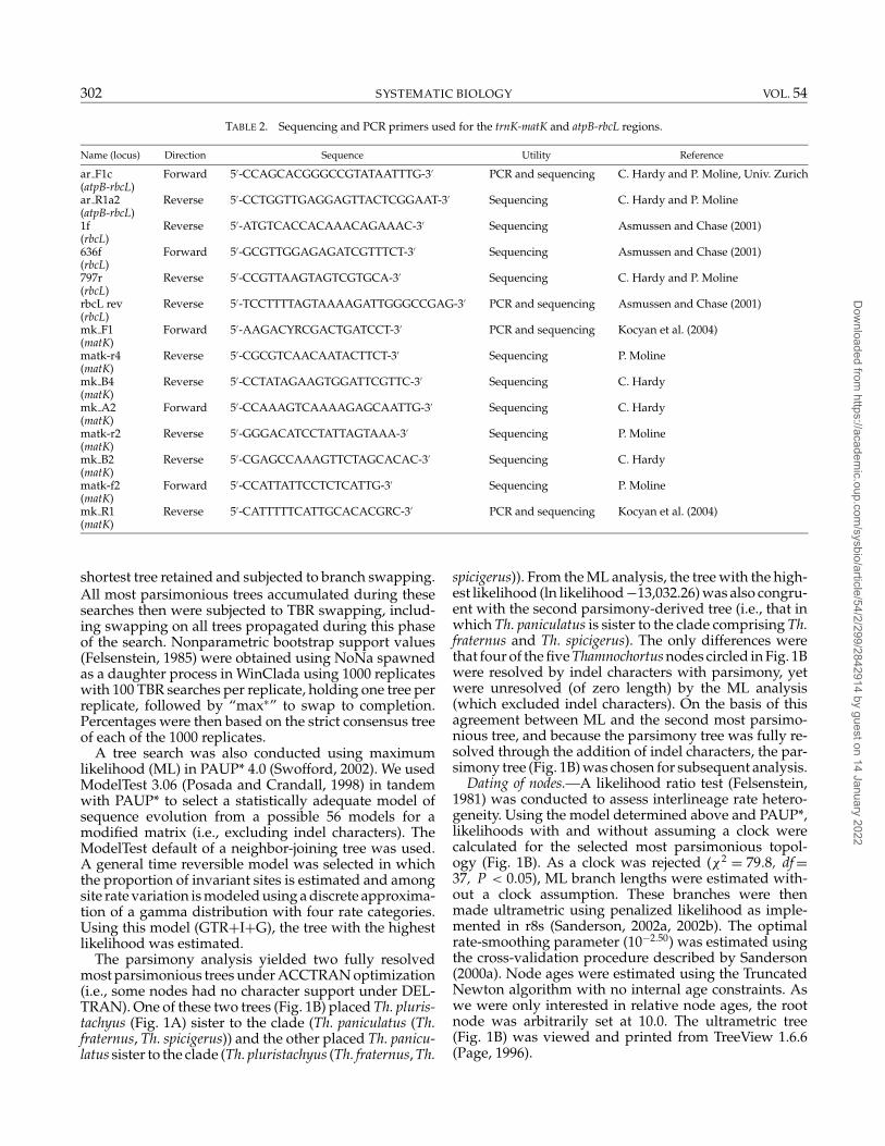
TABLE 2. Sequencing and PCR primers used for the trnK-matK and atpB-rbcL regions.

Name (locus) Direction Sequence Utility Reference

ar F1c Forward 5′-CCAGCACGGGCCGTATAATTTG-3′ PCR and sequencing C. Hardy and P. Moline, Univ. Zurich(atpB-rbcL)ar R1a2 Reverse 5′-CCTGGTTGAGGAGTTACTCGGAAT-3′ Sequencing C. Hardy and P. Moline(atpB-rbcL)1f Reverse 5′-ATGTCACCACAAACAGAAAC-3′ Sequencing Asmussen and Chase (2001)(rbcL)636f Forward 5′-GCGTTGGAGAGATCGTTTCT-3′ Sequencing Asmussen and Chase (2001)(rbcL)797r Reverse 5′-CCGTTAAGTAGTCGTGCA-3′ Sequencing C. Hardy and P. Moline(rbcL)rbcL rev Reverse 5′-TCCTTTTAGTAAAAGATTGGGCCGAG-3′ PCR and sequencing Asmussen and Chase (2001)(rbcL)mk F1 Forward 5′-AAGACYRCGACTGATCCT-3′ PCR and sequencing Kocyan et al. (2004)(matK)matk-r4 Reverse 5′-CGCGTCAACAATACTTCT-3′ Sequencing P. Moline(matK)mk B4 Reverse 5′-CCTATAGAAGTGGATTCGTTC-3′ Sequencing C. Hardy(matK)mk A2 Forward 5′-CCAAAGTCAAAAGAGCAATTG-3′ Sequencing C. Hardy(matK)matk-r2 Reverse 5′-GGGACATCCTATTAGTAAA-3′ Sequencing P. Moline(matK)mk B2 Reverse 5′-CGAGCCAAAGTTCTAGCACAC-3′ Sequencing C. Hardy(matK)matk-f2 Forward 5′-CCATTATTCCTCTCATTG-3′ Sequencing P. Moline(matK)mk R1 Reverse 5′-CATTTTTCATTGCACACGRC-3′ PCR and sequencing Kocyan et al. (2004)(matK)

shortest tree retained and subjected to branch swapping.All most parsimonious trees accumulated during thesesearches then were subjected to TBR swapping, includ-ing swapping on all trees propagated during this phaseof the search. Nonparametric bootstrap support values(Felsenstein, 1985) were obtained using NoNa spawnedas a daughter process in WinClada using 1000 replicateswith 100 TBR searches per replicate, holding one tree perreplicate, followed by “max∗” to swap to completion.Percentages were then based on the strict consensus treeof each of the 1000 replicates.

A tree search was also conducted using maximumlikelihood (ML) in PAUP* 4.0 (Swofford, 2002). We usedModelTest 3.06 (Posada and Crandall, 1998) in tandemwith PAUP* to select a statistically adequate model ofsequence evolution from a possible 56 models for amodified matrix (i.e., excluding indel characters). TheModelTest default of a neighbor-joining tree was used.A general time reversible model was selected in whichthe proportion of invariant sites is estimated and amongsite rate variation is modeled using a discrete approxima-tion of a gamma distribution with four rate categories.Using this model (GTR+I+G), the tree with the highestlikelihood was estimated.

The parsimony analysis yielded two fully resolvedmost parsimonious trees under ACCTRAN optimization(i.e., some nodes had no character support under DEL-TRAN). One of these two trees (Fig. 1B) placed Th. pluris-tachyus (Fig. 1A) sister to the clade (Th. paniculatus (Th.fraternus, Th. spicigerus)) and the other placed Th. panicu-latus sister to the clade (Th. pluristachyus (Th. fraternus, Th.

spicigerus)). From the ML analysis, the tree with the high-est likelihood (ln likelihood −13,032.26) was also congru-ent with the second parsimony-derived tree (i.e., that inwhich Th. paniculatus is sister to the clade comprising Th.fraternus and Th. spicigerus). The only differences werethat four of the five Thamnochortus nodes circled in Fig. 1Bwere resolved by indel characters with parsimony, yetwere unresolved (of zero length) by the ML analysis(which excluded indel characters). On the basis of thisagreement between ML and the second most parsimo-nious tree, and because the parsimony tree was fully re-solved through the addition of indel characters, the par-simony tree (Fig. 1B) was chosen for subsequent analysis.

Dating of nodes.—A likelihood ratio test (Felsenstein,1981) was conducted to assess interlineage rate hetero-geneity. Using the model determined above and PAUP*,likelihoods with and without assuming a clock werecalculated for the selected most parsimonious topol-ogy (Fig. 1B). As a clock was rejected (χ2 = 79.8, df =37, P < 0.05), ML branch lengths were estimated with-out a clock assumption. These branches were thenmade ultrametric using penalized likelihood as imple-mented in r8s (Sanderson, 2002a, 2002b). The optimalrate-smoothing parameter (10−2.50) was estimated usingthe cross-validation procedure described by Sanderson(2000a). Node ages were estimated using the TruncatedNewton algorithm with no internal age constraints. Aswe were only interested in relative node ages, the rootnode was arbitrarily set at 10.0. The ultrametric tree(Fig. 1B) was viewed and printed from TreeView 1.6.6(Page, 1996).

Dow




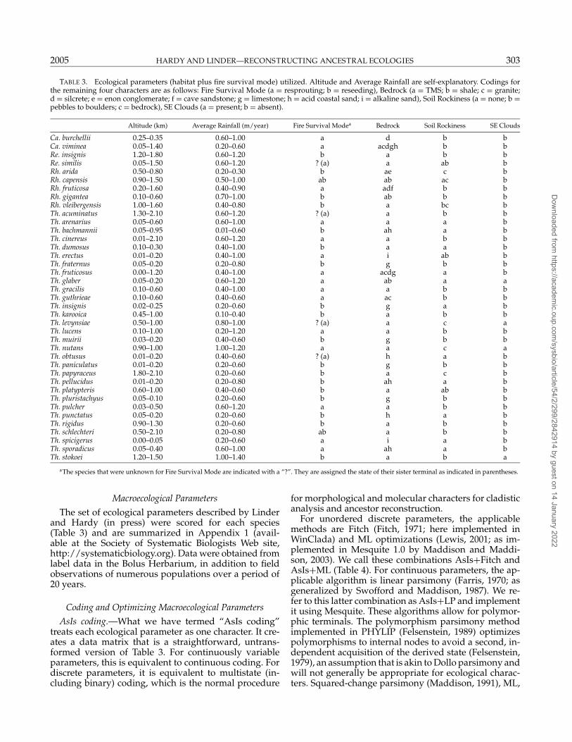
TABLE 3. Ecological parameters (habitat plus fire survival mode) utilized. Altitude and Average Rainfall are self-explanatory. Codings forthe remaining four characters are as follows: Fire Survival Mode (a = resprouting; b = reseeding), Bedrock (a = TMS; b = shale; c = granite;d = silcrete; e = enon conglomerate; f = cave sandstone; g = limestone; h = acid coastal sand; i = alkaline sand), Soil Rockiness (a = none; b =pebbles to boulders; c = bedrock), SE Clouds (a = present; b = absent).

Altitude (km) Average Rainfall (m/year) Fire Survival Modea Bedrock Soil Rockiness SE Clouds

Ca. burchellii 0.25–0.35 0.60–1.00 a d b bCa. viminea 0.05–1.40 0.20–0.60 a acdgh b bRe. insignis 1.20–1.80 0.60–1.20 b a b bRe. similis 0.05–1.50 0.60–1.20 ? (a) a ab bRh. arida 0.50–0.80 0.20–0.30 b ae c bRh. capensis 0.90–1.50 0.50–1.00 ab ab ac bRh. fruticosa 0.20–1.60 0.40–0.90 a adf b bRh. gigantea 0.10–0.60 0.70–1.00 b ab b bRh. vleibergensis 1.00–1.60 0.40–0.80 b a bc bTh. acuminatus 1.30–2.10 0.60–1.20 ? (a) a b bTh. arenarius 0.05–0.60 0.60–1.00 a a a bTh. bachmannii 0.05–0.95 0.01–0.60 b ah a bTh. cinereus 0.01–2.10 0.60–1.20 a a b bTh. dumosus 0.10–0.30 0.40–1.00 b a a bTh. erectus 0.01–0.20 0.40–1.00 a i ab bTh. fraternus 0.05–0.20 0.20–0.80 b g b bTh. fruticosus 0.00–1.20 0.40–1.00 a acdg a bTh. glaber 0.05–0.20 0.60–1.20 a ab a aTh. gracilis 0.10–0.60 0.40–1.00 a a b bTh. guthrieae 0.10–0.60 0.40–0.60 a ac b bTh. insignis 0.02–0.25 0.20–0.60 b g a bTh. karooica 0.45–1.00 0.10–0.40 b a b bTh. levynsiae 0.50–1.00 0.80–1.00 ? (a) a c aTh. lucens 0.10–1.00 0.20–1.20 a a b bTh. muirii 0.03–0.20 0.40–0.60 b g b bTh. nutans 0.90–1.00 1.00–1.20 a a c aTh. obtusus 0.01–0.20 0.40–0.60 ? (a) h a bTh. paniculatus 0.01–0.20 0.20–0.60 b g b bTh. papyraceus 1.80–2.10 0.20–0.60 b a c bTh. pellucidus 0.01–0.20 0.20–0.80 b ah a bTh. platypteris 0.60–1.00 0.40–0.60 b a ab bTh. pluristachyus 0.05–0.10 0.20–0.60 b g b bTh. pulcher 0.03–0.50 0.60–1.20 a a b bTh. punctatus 0.05–0.20 0.20–0.60 b h a bTh. rigidus 0.90–1.30 0.20–0.60 b a b bTh. schlechteri 0.50–2.10 0.20–0.80 ab a b bTh. spicigerus 0.00–0.05 0.20–0.60 a i a bTh. sporadicus 0.05–0.40 0.60–1.00 a ah a bTh. stokoei 1.20–1.50 1.00–1.40 b a b a

aThe species that were unknown for Fire Survival Mode are indicated with a “?”. They are assigned the state of their sister terminal as indicated in parentheses.

Macroecological Parameters

The set of ecological parameters described by Linderand Hardy (in press) were scored for each species(Table 3) and are summarized in Appendix 1 (avail-able at the Society of Systematic Biologists Web site,http://systematicbiology.org). Data were obtained fromlabel data in the Bolus Herbarium, in addition to fieldobservations of numerous populations over a period of20 years.

Coding and Optimizing Macroecological Parameters

AsIs coding.—What we have termed “AsIs coding”treats each ecological parameter as one character. It cre-ates a data matrix that is a straightforward, untrans-formed version of Table 3. For continuously variableparameters, this is equivalent to continuous coding. Fordiscrete parameters, it is equivalent to multistate (in-cluding binary) coding, which is the normal procedure

for morphological and molecular characters for cladisticanalysis and ancestor reconstruction.

For unordered discrete parameters, the applicablemethods are Fitch (Fitch, 1971; here implemented inWinClada) and ML optimizations (Lewis, 2001; as im-plemented in Mesquite 1.0 by Maddison and Maddi-son, 2003). We call these combinations AsIs+Fitch andAsIs+ML (Table 4). For continuous parameters, the ap-plicable algorithm is linear parsimony (Farris, 1970; asgeneralized by Swofford and Maddison, 1987). We re-fer to this latter combination as AsIs+LP and implementit using Mesquite. These algorithms allow for polymor-phic terminals. The polymorphism parsimony methodimplemented in PHYLIP (Felsenstein, 1989) optimizespolymorphisms to internal nodes to avoid a second, in-dependent acquisition of the derived state (Felsenstein,1979), an assumption that is akin to Dollo parsimony andwill not generally be appropriate for ecological charac-ters. Squared-change parsimony (Maddison, 1991), ML,

Dow




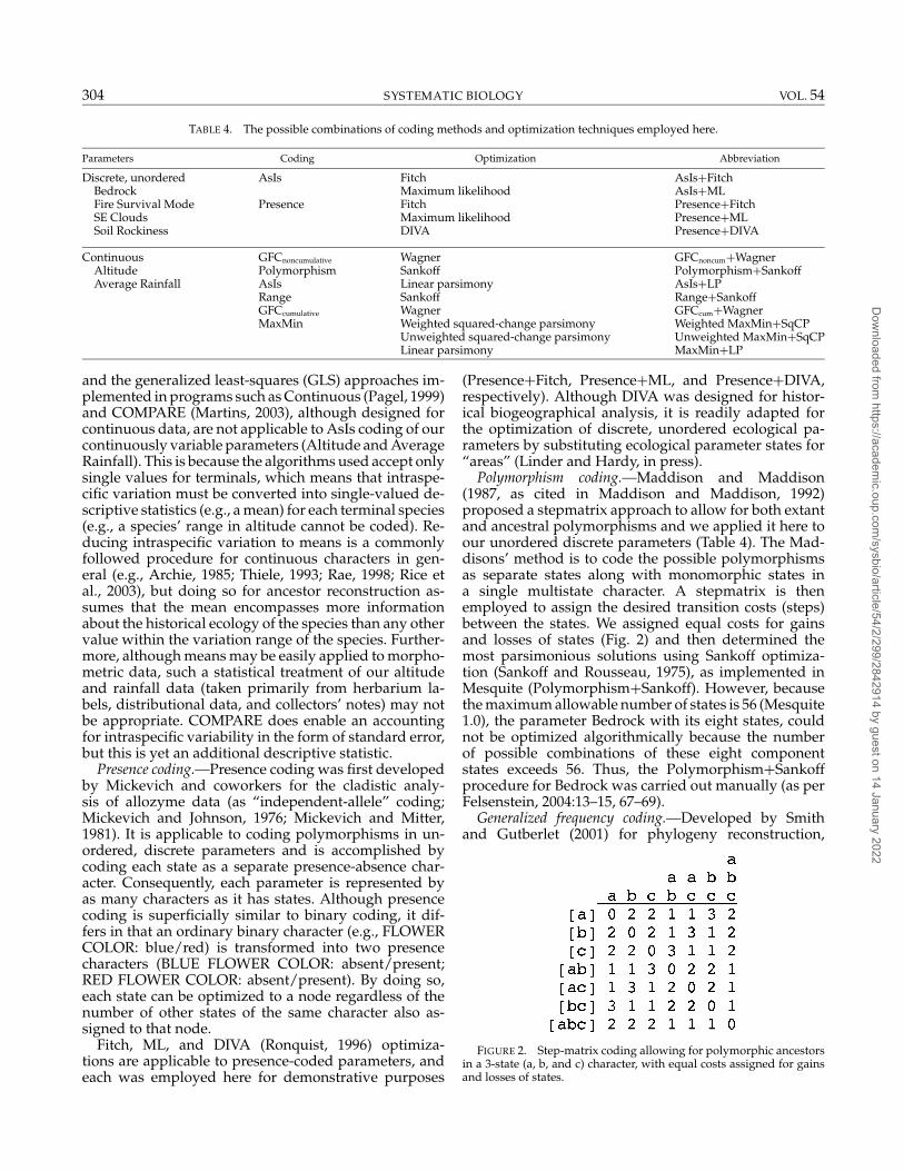
TABLE 4. The possible combinations of coding methods and optimization techniques employed here.

Parameters Coding Optimization Abbreviation

Discrete, unordered AsIs Fitch AsIs+FitchBedrock Maximum likelihood AsIs+MLFire Survival Mode Presence Fitch Presence+FitchSE Clouds Maximum likelihood Presence+MLSoil Rockiness DIVA Presence+DIVA

Continuous GFCnoncumulative Wagner GFCnoncum+WagnerAltitude Polymorphism Sankoff Polymorphism+SankoffAverage Rainfall AsIs Linear parsimony AsIs+LP

Range Sankoff Range+SankoffGFCcumulative Wagner GFCcum+WagnerMaxMin Weighted squared-change parsimony Weighted MaxMin+SqCP

Unweighted squared-change parsimony Unweighted MaxMin+SqCPLinear parsimony MaxMin+LP

and the generalized least-squares (GLS) approaches im-plemented in programs such as Continuous (Pagel, 1999)and COMPARE (Martins, 2003), although designed forcontinuous data, are not applicable to AsIs coding of ourcontinuously variable parameters (Altitude and AverageRainfall). This is because the algorithms used accept onlysingle values for terminals, which means that intraspe-cific variation must be converted into single-valued de-scriptive statistics (e.g., a mean) for each terminal species(e.g., a species’ range in altitude cannot be coded). Re-ducing intraspecific variation to means is a commonlyfollowed procedure for continuous characters in gen-eral (e.g., Archie, 1985; Thiele, 1993; Rae, 1998; Rice etal., 2003), but doing so for ancestor reconstruction as-sumes that the mean encompasses more informationabout the historical ecology of the species than any othervalue within the variation range of the species. Further-more, although means may be easily applied to morpho-metric data, such a statistical treatment of our altitudeand rainfall data (taken primarily from herbarium la-bels, distributional data, and collectors’ notes) may notbe appropriate. COMPARE does enable an accountingfor intraspecific variability in the form of standard error,but this is yet an additional descriptive statistic.

Presence coding.—Presence coding was first developedby Mickevich and coworkers for the cladistic analy-sis of allozyme data (as “independent-allele” coding;Mickevich and Johnson, 1976; Mickevich and Mitter,1981). It is applicable to coding polymorphisms in un-ordered, discrete parameters and is accomplished bycoding each state as a separate presence-absence char-acter. Consequently, each parameter is represented byas many characters as it has states. Although presencecoding is superficially similar to binary coding, it dif-fers in that an ordinary binary character (e.g., FLOWERCOLOR: blue/red) is transformed into two presencecharacters (BLUE FLOWER COLOR: absent/present;RED FLOWER COLOR: absent/present). By doing so,each state can be optimized to a node regardless of thenumber of other states of the same character also as-signed to that node.

Fitch, ML, and DIVA (Ronquist, 1996) optimiza-tions are applicable to presence-coded parameters, andeach was employed here for demonstrative purposes

(Presence+Fitch, Presence+ML, and Presence+DIVA,respectively). Although DIVA was designed for histor-ical biogeographical analysis, it is readily adapted forthe optimization of discrete, unordered ecological pa-rameters by substituting ecological parameter states for“areas” (Linder and Hardy, in press).

Polymorphism coding.—Maddison and Maddison(1987, as cited in Maddison and Maddison, 1992)proposed a stepmatrix approach to allow for both extantand ancestral polymorphisms and we applied it here toour unordered discrete parameters (Table 4). The Mad-disons’ method is to code the possible polymorphismsas separate states along with monomorphic states ina single multistate character. A stepmatrix is thenemployed to assign the desired transition costs (steps)between the states. We assigned equal costs for gainsand losses of states (Fig. 2) and then determined themost parsimonious solutions using Sankoff optimiza-tion (Sankoff and Rousseau, 1975), as implemented inMesquite (Polymorphism+Sankoff). However, becausethe maximum allowable number of states is 56 (Mesquite1.0), the parameter Bedrock with its eight states, couldnot be optimized algorithmically because the numberof possible combinations of these eight componentstates exceeds 56. Thus, the Polymorphism+Sankoffprocedure for Bedrock was carried out manually (as perFelsenstein, 2004:13–15, 67–69).

Generalized frequency coding.—Developed by Smithand Gutberlet (2001) for phylogeny reconstruction,

FIGURE 2. Step-matrix coding allowing for polymorphic ancestorsin a 3-state (a, b, and c) character, with equal costs assigned for gainsand losses of states.

Dow




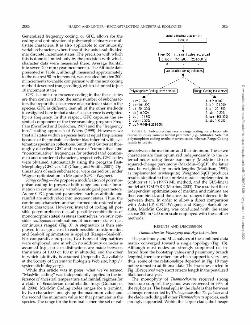
Generalized frequency coding, or GFC, allows for thecoding and optimization of polymorphic binary or mul-tistate characters. It is also applicable to continuouslyvariable characters, where the additive axis is subdividedinto discrete increment states. The precision with whichthis is done is limited only by the precision with whichcharacter data were measured (here, Average Rainfallinto seven 200-mm/year increments). The Altitude datapresented in Table 1, although measured approximatelyto the nearest 50-m increment, was recoded into ten 200-m increments to enable comparison with the next codingmethod described (range coding), which is limited to just10 increment states.

GFC is similar to presence coding in that these statesare then converted into the same number of subcharac-ters that report the occurrence of a particular state in thespecies. GFC is different than all of the other methodsinvestigated here in that a state’s occurrence is weightedby its frequency. In this respect, GFC captures the es-sential component of the tree-searching program Freq-Pars (Swofford and Berlocher, 1987) and the “frequencybins”–coding approach of Wiens (1995). However, wetreat all states within a species here at equal frequenciesbecause of the probable collector bias inherent with sys-tematics specimen collections. Smith and Gutberlet thor-oughly described GFC and its use of “cumulative” and“noncumulative” frequencies for ordered (and continu-ous) and unordered characters, respectively. GFC codeswere obtained automatically using the program Fast-MorphologyGFC ver. 1.0 (Chang and Smith, 2001). Op-timizations of each subcharacter were carried out underWagner optimization in Mesquite (GFC+Wagner).

Range coding.—We propose a modification of polymor-phism coding to preserve both range and order infor-mation in continuously variable ecological parameters.As for GFC, gradient parameters such as altitude andrainfall are subdivided into increment states. Thus, thecontinuous characters are transformed into ordered mul-tistate characters. However, instead of coding all pos-sible polymorphisms (i.e., all possible combinations ofmonomorphic states) as states themselves, we only con-sider contiguous combinations of increment states (i.e.,continuous ranges) (Fig. 3). A stepmatrix is then em-ployed to assign a cost to each possible transformationand Sankoff optimization is applied (Range+Sankoff).For comparative purposes, two types of stepmatriceswere employed, one in which no additivity or order isassumed (e.g., no cost distinctions are made betweentransitions of 1000 or 100 m in altitude), and the otherin which additivity is assumed (Appendix 2, availableat the Society of Systematic Biologists Web site, http://systematicbiology.org).

While this article was in press, what we’ve termed“MaxMin coding” was independently applied in the in-ference of ancestral temperature and rainfall regimes fora clade of Ecuadorian dendrobadid frogs (Graham etal. 2004). MaxMin Coding codes ranges for a terminalby two characters: one giving the maximum value andthe second the minimum value for that parameter in thespecies. The range for the terminal is then the set of val-

FIGURE 3. Polymorphism versus range coding for a hypotheti-cal continuously variable habitat parameter (e.g., Altitude). Note thatpolymorphism coding results in seven states, whereas Range Codingresults in just six.

ues between the maximum and the minimum. These twocharacters are then optimized independently to the in-ternal nodes using linear parsimony (MaxMin+LP) orsquared-change parsimony (MaxMin+SqCP), the lattermay be weighted by branch lengths (Maddison, 1991;as implemented in Mesquite). Weighted SqCP producesresults identical to the simplest models implemented inSchluter et al.’s (1997) ML method, and the GLS-linearmodel of COMPARE (Martins, 2003). The results of theseindependent optimizations of maxima and minima arethen combined, and the ancestral ranges inferred to liebetween them. In order to allow a direct comparisonwith AsIs+LP, GFC+Wagner, and Range+Sankoff re-sults, MaxMin Coding was conducted with the samecoarse 200 m/200 mm scale employed with these othermethods.

RESULTS AND DISCUSSION

Thamnochortus Phylogeny and Age Estimation

The parsimony and ML analyses of the combined datamatrix converged toward a single topology (Fig. 1B).Although most nodes are strongly supported (as in-ferred from the bootstrap values and parsimony branchlengths), there are others for which support is very low;thus, some of the relationships depicted in Fig. 1B maynot be robust to additional data. The branches circled inFig. 1B received very short or zero length in the penalizedlikelihood analysis.

The monophyly of Thamnochortus received strongbootstrap support: the genus was recovered in 99% ofthe replicates. The basal split in the clade is that betweena lineage represented by Th. levynsiae plus Th. pulcher andthe clade including all other Thamnochortus species, eachstrongly supported. Within this larger clade, the lineage

Dow




comprising Th. gracilis and Th. nutans is sister to the re-maining Thamnochortus species.

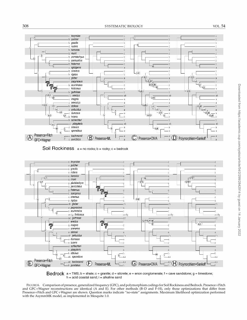
Within this remaining group, the clade including bothTh. muirii and Th. spicigerus received strong bootstrapsupport (94%) and is the most distinctive of all cladesin Thamnochortus in terms of habitat, occurring at lowelevations and primarily on limestone soils or the al-kaline coastal sands of the western Cape (Fig. 6E). Theone exception to this is Th. karooica, which is found onsandstone in the dry fynbos in the low to middle eleva-tions of the Little Karoo Mountains and along the inlandside of the Langeberg. The sister-group relationship ofthis alkaline-soil clade to the remaining Thamnochortusreceived no bootstrap support and was resolved only bya single (substitution) character.

Of the remaining four major clades, the one includingboth Th. cinereus and Th. fruticosus is sister, albeit with nobootstrap support, to a clade that includes the other three.Within the latter, the clade comprising Th. guthrieae, Th.erectus, and Th. insignis is sister to the lineage comprisingthe remaining two major clades. This latter clade com-prises the sister groups (Th. arenarius(Th. stokoei(Th. pel-lucidus(Th. dumosus, Th. lucens)))) and (Th. schlechteri(Th.platypteris((Th. bachmannii, Th. punctatus)(Th. obtusus, Th.

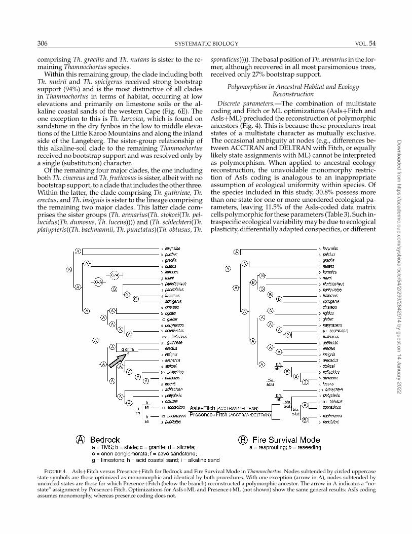
FIGURE 4. AsIs+Fitch versus Presence+Fitch for Bedrock and Fire Survival Mode in Thamnochortus. Nodes subtended by circled uppercasestate symbols are those optimized as monomorphic and identical by both procedures. With one exception (arrow in A), nodes subtended byuncircled states are those for which Presence+Fitch (below the branch) reconstructed a polymorphic ancestor. The arrow in A indicates a “no-state” assignment by Presence+Fitch. Optimizations for AsIs+ML and Presence+ML (not shown) show the same general results: AsIs codingassumes monomorphy, whereas presence coding does not.

sporadicus)))). The basal position of Th. arenarius in the for-mer, although recovered in all most parsimonious trees,received only 27% bootstrap support.

Polymorphism in Ancestral Habitat and EcologyReconstruction

Discrete parameters.—The combination of multistatecoding and Fitch or ML optimizations (AsIs+Fitch andAsIs+ML) precluded the reconstruction of polymorphicancestors (Fig. 4). This is because these procedures treatstates of a multistate character as mutually exclusive.The occasional ambiguity at nodes (e.g., differences be-tween ACCTRAN and DELTRAN with Fitch, or equallylikely state assignments with ML) cannot be interpretedas polymorphism. When applied to ancestral ecologyreconstruction, the unavoidable monomorphy restric-tion of AsIs coding is analogous to an inappropriateassumption of ecological uniformity within species. Ofthe species included in this study, 30.8% possess morethan one state for one or more unordered ecological pa-rameters, leaving 11.5% of the AsIs-coded data matrixcells polymorphic for these parameters (Table 3). Such in-traspecific ecological variability may be due to ecologicalplasticity, differentially adapted conspecifics, or different

Dow




community-level species interactions in different partsof a species’ range. Regardless of the biological basisfor such intraspecific ecological variability, optimizationprocedures that account for this are preferable.

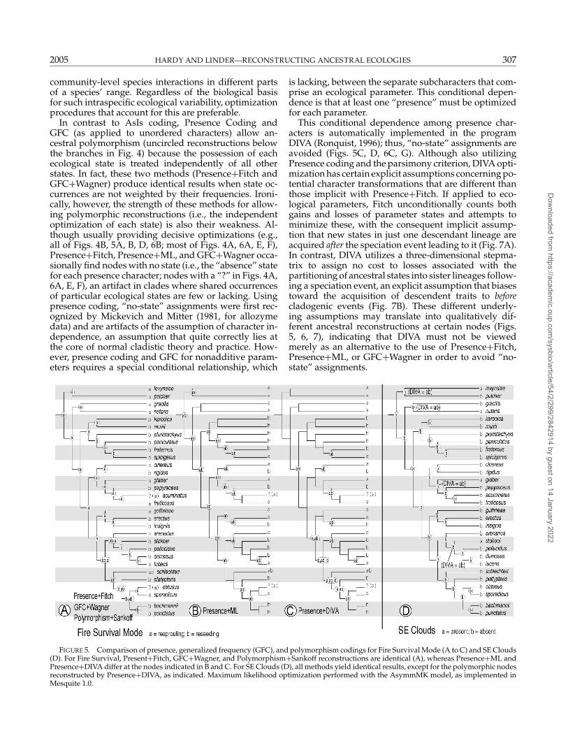
In contrast to AsIs coding, Presence Coding andGFC (as applied to unordered characters) allow an-cestral polymorphism (uncircled reconstructions belowthe branches in Fig. 4) because the possession of eachecological state is treated independently of all otherstates. In fact, these two methods (Presence+Fitch andGFC+Wagner) produce identical results when state oc-currences are not weighted by their frequencies. Ironi-cally, however, the strength of these methods for allow-ing polymorphic reconstructions (i.e., the independentoptimization of each state) is also their weakness. Al-though usually providing decisive optimizations (e.g.,all of Figs. 4B, 5A, B, D, 6B; most of Figs. 4A, 6A, E, F),Presence+Fitch, Presence+ML, and GFC+Wagner occa-sionally find nodes with no state (i.e., the “absence” statefor each presence character; nodes with a “?” in Figs. 4A,6A, E, F), an artifact in clades where shared occurrencesof particular ecological states are few or lacking. Usingpresence coding, “no-state” assignments were first rec-ognized by Mickevich and Mitter (1981, for allozymedata) and are artifacts of the assumption of character in-dependence, an assumption that quite correctly lies atthe core of normal cladistic theory and practice. How-ever, presence coding and GFC for nonadditive param-eters requires a special conditional relationship, which

FIGURE 5. Comparison of presence, generalized frequency (GFC), and polymorphism codings for Fire Survival Mode (A to C) and SE Clouds(D). For Fire Survival, Present+Fitch, GFC+Wagner, and Polymorphism+Sankoff reconstructions are identical (A), whereas Presence+ML andPresence+DIVA differ at the nodes indicated in B and C. For SE Clouds (D), all methods yield identical results, except for the polymorphic nodesreconstructed by Presence+DIVA, as indicated. Maximum likelihood optimization performed with the AsymmMK model, as implemented inMesquite 1.0.

is lacking, between the separate subcharacters that com-prise an ecological parameter. This conditional depen-dence is that at least one “presence” must be optimizedfor each parameter.

This conditional dependence among presence char-acters is automatically implemented in the programDIVA (Ronquist, 1996); thus, “no-state” assignments areavoided (Figs. 5C, D, 6C, G). Although also utilizingPresence coding and the parsimony criterion, DIVA opti-mization has certain explicit assumptions concerning po-tential character transformations that are different thanthose implicit with Presence+Fitch. If applied to eco-logical parameters, Fitch unconditionally counts bothgains and losses of parameter states and attempts tominimize these, with the consequent implicit assump-tion that new states in just one descendant lineage areacquired after the speciation event leading to it (Fig. 7A).In contrast, DIVA utilizes a three-dimensional stepma-trix to assign no cost to losses associated with thepartitioning of ancestral states into sister lineages follow-ing a speciation event, an explicit assumption that biasestoward the acquisition of descendent traits to beforecladogenic events (Fig. 7B). These different underly-ing assumptions may translate into qualitatively dif-ferent ancestral reconstructions at certain nodes (Figs.5, 6, 7), indicating that DIVA must not be viewedmerely as an alternative to the use of Presence+Fitch,Presence+ML, or GFC+Wagner in order to avoid “no-state” assignments.

Dow




FIGURE 6. Comparison of presence, generalized frequency (GFC), and polymorphism codings for Soil Rockiness and Bedrock. Presence+Fitchand GFC+Wagner reconstructions are identical (A and E). For other methods (B–D and F–H), only those optimizations that differ fromPresence+Fitch and GFC+Wagner are shown. Question marks indicate “no-state” assignments. Maximum likelihood optimization performedwith the AsymmMK model, as implemented in Mesquite 1.0.

Dow




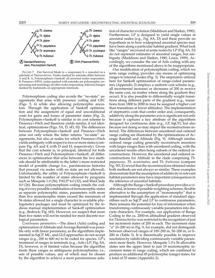
FIGURE 7. Fire Survival Mode (a = resprouter; b = reseeder) in asubclade of Thamnochortus. Nodes marked by asterisks differ betweenA and B. A, Polymorphism+Sankoff: all ancestral nodes resprouters.B, Presence+DIVA, nodes marked with asterisks are polymorphic (re-sprouting and reseeding); all other nodes resprouting. Inferred changesmarked by hashmarks on appropriate internode.

Polymorphism coding also avoids the “no-state” as-signments that arise with presence coding and GFC(Figs. 5, 6) while also allowing polymorphic ances-tors. Through the application of Sankoff optimiza-tion and the assignment of equal and unconditionalcosts for gains and losses of parameter states (Fig. 2),Polymorphism+Sankoff is similar in its cost scheme toPresence+Fitch and therefore yields similar, if not iden-tical, optimizations (Figs. 5A, D, 6D, H). The differencesbetween Polymorphism+Sankoff and Presence+Fitcharise not only where the latter returns “no-state” as-signments, but also at nodes for which Presence+Fitchyields ambiguity with respect to two or more states (com-pare Fig. 6A and E with D and H, respectively). Giventhat the cost scheme is, in principal, identical for bothPresence+Fitch and Polymorphism+Sankoff, all differ-ences in optimization that arise between the two meth-ods should be attributable to the latter’s more restrictedmodel of possible change (i.e., parsimonious historiesthat proceed via nodes with no state are not allowed).Unfortunately, the utility of Polymorphism+Sankoff islimited by the number of states allowed by programssuch as Mesquite 1.0 (56), PAUP∗4.0 (32), and MacClade4.0 (26). Because polymorphism coding entails the cod-ing of every possible combination of monomorphic statesas separate polymorphic states, parameters with morethan five monomorphic states exceed the maximum of56 states allowed for a single character in available phy-logenetics packages and must be optimized by the te-dious manual implementation of Sankoff optimization(e.g., Bedrock; Fig. 6H). However, we suspect that morethan five states will not be needed for most discrete eco-logical parameters.

Continuous parameters.—The direct (AsIs) coding andoptimization of Altitude and Average Rainfall was possi-ble only with linear parsimony, as the algorithms imple-mented in SqCP, ML, and GLS approaches do not acceptranges (e.g., 200 to 600 m) to be coded for species. LP’streatment of ranges in terminals (e.g., AsIs+LP; Fig. 8A,D), however, is of limited value because the algorithmtreats these ranges as ambiguous polymorphisms; i.e.,sets of possible values, any of which may be chosenby the algorithm to achieve a most parsimonious solu-

tion of character evolution (Maddison and Slatkin, 1990).Furthermore, LP is designed to yield single values atancestral nodes (e.g., Fig. 8A, D) and these provide nohypothesis as to how widespread ancestral species mayhave been along a particular habitat gradient. What looklike “ranges” recovered at some nodes by LP (Fig. 8A, D)do not represent estimates of ancestral ranges, but am-biguity (Maddison and Slatkin, 1990; Losos, 1999). Ac-cordingly, we consider the use of AsIs coding with anyof the algorithms mentioned above to be inappropriate.

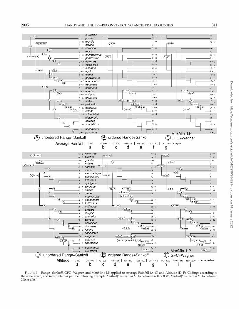
Our modification of polymorphism coding, which weterm range coding, provides one means of optimizingranges to internal nodes (Fig. 3). The stepmatrix utilizedhere for Sankoff optimization of range-coded parame-ters (Appendix 2) employs a uniform cost scheme (e.g.,all incremental increases or decreases of 200 m receivethe same cost, no matter where along the gradient theyoccur). It is also possible to differentially weight transi-tions along different parts of the gradient (e.g., transi-tions from 1800 to 2000 m may be assigned a higher costthan transitions at lower altitudes). The implementationof stepmatrix costs that confer order and, consequently,additivity along the parameter axis is significant not onlybecause it captures a key attribute of the algorithmsdesigned for continuous data (e.g., LP, SqCP), but alsobecause not doing so may impact the reconstructions in-ferred. The differences between unordered and orderedrange coding are illustrated by the optimizations of Av-erage Rainfall and Altitude (Fig. 9). Although similar,ordered range coding generally reconstructs ancestorswith larger ranges than with unordered coding, with theunordered results often being subsets of the ordered re-constructions. However, the unordered and ordered re-constructions for Altitude in the clade comprising Th.papyraceus, Th. acuminatus, and Th. fruticosus (compareFig. 9D, E) reveal that the reconstructions obtained underboth methods are not always so similar. These examplesdemonstrate that the assumption of additivity in relevanthabitat parameters may have important consequences inthe inference of ancestral habitats.

Although the Range+Sankoff procedure provides a vi-able and, in terms of possible weighting schemes, flexiblealternative to the assumption of “monomorphy” that isimplemented through the application of standard algo-rithms such as SqCP and LP to continuous parameters,there remains the potential for loss of information whentransforming continuously variable parameters into dis-crete characters. For example, our application of RangeCoding to the ca. 2000-m altitudinal gradient observedfor Thamnochortus was restricted to the recognition of justten increment states of 200 m each. The increment state“a” (0–200 m) in Fig. 9, for example, did not distinguishbetween observed ranges of 100–200 m, 50–200 m, or 0–200 m (Table 3). It is theoretically possible to improveresolution by subdividing continuously variable param-eters more finely. However, Mesquite 1.0’s 56 allowablestates sets the upper limit to just 10 monomorphic in-crement states in range coding, which are combined toproduce an additional 45 polymorphic (range) states, fora total of 55 states (Appendix 2).

Dow




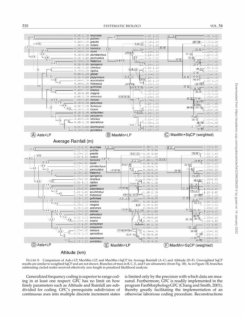
FIGURE 8. Comparison of AsIs+LP, MaxMin+LP, and MaxMin+SqCP for Average Rainfall (A–C) and Altitude (D–F). Unweighted SqCPresults are similar to weighted SqCP and are not shown. Branches of trees in B, C, E, and F are ultrametric (from Fig. 1B). As in Figure 1B, branchessubtending circled nodes received effectively zero length in penalized likelihood analysis.

Generalized frequency coding is superior to range cod-ing in at least one respect: GFC has no limit on howfinely parameters such as Altitude and Rainfall are sub-divided for coding. GFC’s prerequisite subdivision ofcontinuous axes into multiple discrete increment states

is limited only by the precision with which data are mea-sured. Furthermore, GFC is readily implemented in theprogram FastMorphologyGFC (Chang and Smith, 2001),thereby greatly facilitating the implementation of anotherwise laborious coding procedure. Reconstructions

Dow




FIGURE 9. Range+Sankoff, GFC+Wagner, and MaxMin+LP applied to Average Rainfall (A–C) and Altitude (D–F). Codings according tothe scale given, and interpreted as per the following example: “a-(b-d)” is read as “0 to between 400 or 800”; “a(-b-d)” is read as “0 to between200 or 800.”

Dow




implied by GFC+Wagner are, however, tedious to inter-pret, because reconstructions must be inferred by sum-ming across multiple subcharacters on a node-by-nodebasis. This is because GFC was developed as a way onlyto extract information from polymorphic (and continu-ously variable) characters for cladistic analysis: we havemerely co-opted it here for the inference of ancestralstates. The labor involved with ancestor inference us-ing GFC+Wagner increases drastically with increasingsubdivision of continuously variable character axes. Al-though we have not done so here on account of a per-ceived bias in the habitat distributions implied by sys-tematics specimen collections, the capacity of GFC toaccommodate species’ frequency distributions may beseen by some investigators as an additional desirable at-tribute of the method.

MaxMin coding has several advantages over bothrange coding and GFC. First, it is not necessary to trans-form continuously variable data into discrete incrementstates. As demonstrated above, the number of incrementstates (and therefore precision) possible using range cod-ing is limited. Although the precision of axis subdivisionusing GFC is not limiting, inference of ancestral rangesbecomes increasingly tedious with increasing subdivi-sion for the reason described above. MaxMin codingrequires that inferences be made simply by summingacross just two subcharacters (the minimum and themaximum). Our results suggest that the added tediumassociated with GFC comes without added benefit: GFCand MaxMin produced identical results under parsi-mony when ranges, rather than frequency distributions,were coded (Fig. 9C, F).

A second advantage that MaxMin has over both rangecoding and GFC is that it allows for the applicationof SqCP or more powerful GLS or ML approaches(Pagel, 1999; Martins and Hansen, 1997; Martins,1999) designed to account for branch lengths duringoptimization. These algorithms/models implementvariations upon an implicit (SqCP) or explicit (ML, GLS)assumption that continuous character evolution can bemodeled as a stochastic process (Maddison, 1991; Mar-tins, 1999). The probability of change along any branchis proportional to its length. One possible objection tomodeling ecological change as a stochastic process is thepossibility that many ecological attributes are under se-lective pressures and evolve under the influence of otherforces such as divergent or stabilizing selection (Losos,1999; Martins et al., 2002 and references cited therein).Indeed, LP’s tendency of reconstructing most brancheswith no change and relatively few branches with largeamounts of change has been likened to an implicit, andperhaps appropriate, model of stabilizing selection withoccasional adaptive shifts (Losos, 1999). As appealingas this assumption implicit with LP might be, recenttheoretical and algorithmic progress has introduced thepotential for modeling the influence of selection (e.g.,GLS-exponential and the Phylogenetic Mixed Model ofMartins, 2003, and Housworth et al., 2004). The efficacywith which such forces can be modeled and used for ac-curate reconstructions is not yet clear (compare Martins,

1999 with Martins et al., 2002). However, the increasingavailability of a variety of parameter-driven, statisticallybased evolutionary models points toward the powerfulprospect of objectively testing and selecting a modelappropriate for one’s study group.

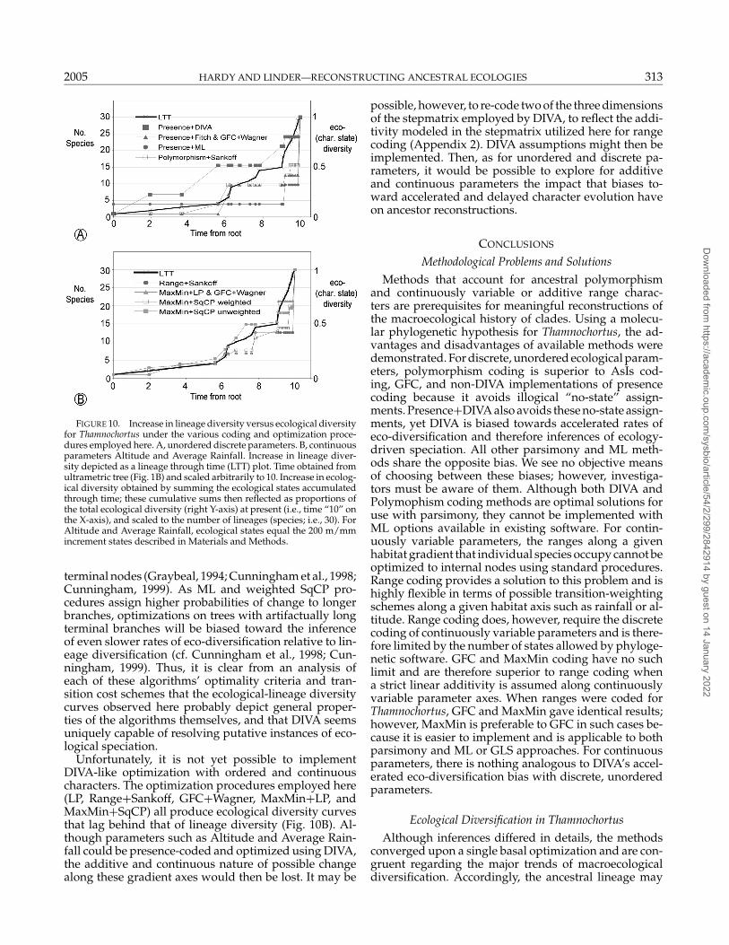
Timing of Ecological Diversification

A neglected aspect of ancestor reconstruction is the im-pact that alternative algorithms have on the rate and tim-ing of character evolution inferred (Linder and Hardy, inpress). The rate and timing of eco-diversification rela-tive to lineage (species) diversification are of particularinterest in the pursuit of identifying the forces drivingspeciation. If eco-diversification can be shown to pre-cede lineage diversification in particular clades, thenthere is support for the hypothesis that ecological fac-tors may be driving speciation. The converse would bethat eco-diversification follows and, by implication, doesnot drive lineage diversification. Our results reveal that,for the same data and phylogeny, either scenario can bedemonstrated, depending on the optimization methodemployed, and we see no a priori means of choosing be-tween these biases. Using Presence+DIVA on unorderedparameters, the accumulation of ecological diversity pre-cedes that of lineage diversity (Fig. 10A). In contrast, allother combinations produce ecological diversity curvesthat lag behind lineage diversity (Fig. 10A, B). Thesebiases are especially evident when trend lines are fit-ted to the data plotted in Fig. 10 (not shown). Amongthe parsimony-based optimizations, this dichotomy canbe understood as a consequence of different transitioncost schemes. Schemes that assign equal and uncondi-tional costs to gains and losses of states (Fitch and, asimplemented here, Sankoff) will tend to place the ac-quisition of new ecological states on branches followingspeciation events. In contrast, DIVA employs a three-dimensional stepmatrix to assign no cost to “losses” asso-ciated with the partitioning of ancestral states into sisterlineages following a speciation event. Thus, DIVA biasestoward inferences of ecological vicariance or ecologicalspeciation (Ehrlich and Raven, 1969; Andersson, 1990;Schluter, 2000; Levin, 2000, 2003), where the acquisitionof states exclusive to each of two descendant sister lin-eages is accelerated to the ancestral lineage, followed bythe splitting of that lineage along these ecological bound-aries reflected in the descendants (Fig. 7). Our resultsalso demonstrate that ML behaves like other non-DIVAparsimony algorithms with respect to the relative ratesof ecological and lineage diversification. In fact, withincoding types (e.g., Presence, MaxMin), optimizationsthat account for branch lengths (ML and, for continuousparameters, weighted SqCP) produce the slowest eco-logical diversity curves, all of which lay below thatof lineage diversity (Fig. 10). Furthermore, the delayin eco-diversification inferred by procedures that usebranch lengths may be exacerbated by branch length es-timates based on saturated genetic loci when, despiteemploying reasonable models of sequence evolution,ML may fail to fully correct the bias toward the arti-factual inference of shorter internal nodes and longer

Dow




FIGURE 10. Increase in lineage diversity versus ecological diversityfor Thamnochortus under the various coding and optimization proce-dures employed here. A, unordered discrete parameters. B, continuousparameters Altitude and Average Rainfall. Increase in lineage diver-sity depicted as a lineage through time (LTT) plot. Time obtained fromultrametric tree (Fig. 1B) and scaled arbitrarily to 10. Increase in ecolog-ical diversity obtained by summing the ecological states accumulatedthrough time; these cumulative sums then reflected as proportions ofthe total ecological diversity (right Y-axis) at present (i.e., time “10” onthe X-axis), and scaled to the number of lineages (species; i.e., 30). ForAltitude and Average Rainfall, ecological states equal the 200 m/mmincrement states described in Materials and Methods.

terminal nodes (Graybeal, 1994; Cunningham et al., 1998;Cunningham, 1999). As ML and weighted SqCP pro-cedures assign higher probabilities of change to longerbranches, optimizations on trees with artifactually longterminal branches will be biased toward the inferenceof even slower rates of eco-diversification relative to lin-eage diversification (cf. Cunningham et al., 1998; Cun-ningham, 1999). Thus, it is clear from an analysis ofeach of these algorithms’ optimality criteria and tran-sition cost schemes that the ecological-lineage diversitycurves observed here probably depict general proper-ties of the algorithms themselves, and that DIVA seemsuniquely capable of resolving putative instances of eco-logical speciation.

Unfortunately, it is not yet possible to implementDIVA-like optimization with ordered and continuouscharacters. The optimization procedures employed here(LP, Range+Sankoff, GFC+Wagner, MaxMin+LP, andMaxMin+SqCP) all produce ecological diversity curvesthat lag behind that of lineage diversity (Fig. 10B). Al-though parameters such as Altitude and Average Rain-fall could be presence-coded and optimized using DIVA,the additive and continuous nature of possible changealong these gradient axes would then be lost. It may be

possible, however, to re-code two of the three dimensionsof the stepmatrix employed by DIVA, to reflect the addi-tivity modeled in the stepmatrix utilized here for rangecoding (Appendix 2). DIVA assumptions might then beimplemented. Then, as for unordered and discrete pa-rameters, it would be possible to explore for additiveand continuous parameters the impact that biases to-ward accelerated and delayed character evolution haveon ancestor reconstructions.

CONCLUSIONS

Methodological Problems and Solutions

Methods that account for ancestral polymorphismand continuously variable or additive range charac-ters are prerequisites for meaningful reconstructions ofthe macroecological history of clades. Using a molecu-lar phylogenetic hypothesis for Thamnochortus, the ad-vantages and disadvantages of available methods weredemonstrated. For discrete, unordered ecological param-eters, polymorphism coding is superior to AsIs cod-ing, GFC, and non-DIVA implementations of presencecoding because it avoids illogical “no-state” assign-ments. Presence+DIVA also avoids these no-state assign-ments, yet DIVA is biased towards accelerated rates ofeco-diversification and therefore inferences of ecology-driven speciation. All other parsimony and ML meth-ods share the opposite bias. We see no objective meansof choosing between these biases; however, investiga-tors must be aware of them. Although both DIVA andPolymophism coding methods are optimal solutions foruse with parsimony, they cannot be implemented withML options available in existing software. For contin-uously variable parameters, the ranges along a givenhabitat gradient that individual species occupy cannot beoptimized to internal nodes using standard procedures.Range coding provides a solution to this problem and ishighly flexible in terms of possible transition-weightingschemes along a given habitat axis such as rainfall or al-titude. Range coding does, however, require the discretecoding of continuously variable parameters and is there-fore limited by the number of states allowed by phyloge-netic software. GFC and MaxMin coding have no suchlimit and are therefore superior to range coding whena strict linear additivity is assumed along continuouslyvariable parameter axes. When ranges were coded forThamnochortus, GFC and MaxMin gave identical results;however, MaxMin is preferable to GFC in such cases be-cause it is easier to implement and is applicable to bothparsimony and ML or GLS approaches. For continuousparameters, there is nothing analogous to DIVA’s accel-erated eco-diversification bias with discrete, unorderedparameters.

Ecological Diversification in Thamnochortus

Although inferences differed in details, the methodsconverged upon a single basal optimization and are con-gruent regarding the major trends of macroecologicaldiversification. Accordingly, the ancestral lineage may

Dow




have been a post-fire resprouting species distributedon rocky and well-drained, sandstone-derived soils atlower-middle elevations in regions characterized bymoderate levels of yearly (particularly winter) rainfalland negligible contributions of moisture from cloudsduring the summer months (Figs. 5 to 9). This specieswould have been distributed in habitats much like thoseexisting throughout much of the southwestern Capemountains today.

With respect to fire survival, post-fire reseeders arederived within Thamnochortus. DIVA infers the same po-larity to this transformation, but the transformations toreseeding proceeded via a polymorphic intermediate lin-eage on at least eight separate occasions, each invokinga hypothesis of vicariant speciation with respect to thesetwo life-history traits. Presence+ML inferences are con-trary to parsimony inferences in suggesting that all an-cestral species were polymorphic for Fire Survival Modeand that loss of either of the two traits occurred re-cently and independently in several lineages. However,non-DIVA implementations of presence coding, such asPresence+ML, are known to be prone to illogical, arti-factual reconstructions are therefore suboptimal.

With regards to moisture regime, all methods pointto a shift from regions of moderate yearly rainfall (ca.600–1000 mm/year) to regions of lower rainfall (200–600 mm/year) in the Th. muirii—Th. spicigerus lineage.Independently, the Th. platypteris–Th. bachmannii lin-eage experienced a shift to a lower and narrower rain-fall regime (ca. 400–700 mm/year). The occurrences ofspecies in winter rainfall regions that receive substan-tial amounts of summer moisture from clouds off the In-dian Ocean are recently and separately derived in severallineages. Expectedly, DIVA suggests that these summer(southeast) cloud habitat shifts took place via intermedi-ate lineages that existed in both habitats. All parsimonymethods suggest that lineages found on deep, rockless,and summer-dry soils (Appendix 1) are derived fromlineages occurring on well-drained, rocky soils.

Finally, all methods also point to occurrences at lower-middle elevations (<1000 m) on sandstone-derived soilsas plesiomorphic. Subsequent shifts to lower, includingcoastal, elevations have occurred independently in boththe Th. guthrieae–Th. erectus and Th. muirii–Th. spicigeruslineages. Both were associated with a shift from acidicsandstone-derived soils to limestone or otherwise alka-line soils.

ACKNOWLEDGMENTS

Support for this research was generously provided by the SwissNational Fund, the Swiss Academy of Natural Sciences, Georges andAntoine Claraz-Schenkung, and The National Geographic Society. Wethank The Western Cape Nature Conservation Board for the permis-sion to collect the plants, Frank Rutschmann for assistance with the pe-nalized likelihood analysis, Philip Moline for providing unpublishedprimer sequences, and Philip Moline, Terry Trinder-Smith, and the staffat the Bolus Herbarium for facilitating fieldwork in the Cape. ChloeGalley, Timo van der Niet, Roderic Page, Todd Oakley, and two anony-mous reviewers provided helpful comments on an earlier draft of thisarticle. We also thank Emilia Martins for helpful correspondence re-garding COMPARE.

REFERENCES

Andersson, L. 1990. The driving force: Species concepts and ecology.Taxon 39:375–382.

Archie, J. W. 1985. Methods for coding variable morphological featuresfor numerical taxonomic analysis. Syst. Zool. 34:326–345.

Asmussen, C. B., and M. W. Chase. 2001. Coding and noncoding plastidDNA in palm systematics. Am. J. Bot. 88:1103–1117.

Butler, M. A., and J. B. Losos. 1997. Testing for unequal amounts of evo-lution in a continuous character on different branches of a phyloge-netic tree using linear and squared-change parsimony: An exampleusing Lesser Antillean Anolis lizards. Evolution 51:1623–1635.

Campbell, B. M. 1983. Montane plant environments in the FynbosBiome. Bothalia 14:283–298.

Change, V., and E. N. Smith. 2001. FastMorphologyGFC version 1.0.http://www3.uta.edu/faculty/ensmith.

Chase, M. W., and V. A. Albert. 1998. A perspective on the contribu-tion of plastid rbcL DNA sequences to angiosperm phylogenetics.Pages 488–507 in Molecular systematics of plants II: DNA sequenc-ing (D. E. Soltis, P. S. Soltis, and J. J. Doyle, eds.). Kluwer AcademicPublishers, Boston, Massachusetts.

Cowling, R. M. 1987. Fire and its role in coexistence and speciation inGondwanan shrublands. S. African J. Sci. 83:106–112.

Cowling, R. M., P. W. Rundel, B. B. Lamont, M. K. Arroyo, and M.Arianoutsou. 1996. Plant diversity in Mediterranean-climate regions.Trends Ecol. Evol. 11:362–366.

Cunningham, C. W. 1999. Some limitations of ancestral character-statereconstruction when testing evolutionary hypotheses. Syst. Biol.48:665–674.

Cunningham, C. W., K. E. Omland, and T. H. Oakley. 1998. Reconstruct-ing ancestral character states: A critical reappraisal. Trends Ecol.Evol. 13:361–366.

Donoghue, M. J., and D. D. Ackerly. 1996. Phylogenetic uncertaintiesand sensitivity analysis in comparative biology. Philos. Trans. R. Soc.Lond. B 351:1241–1249.

Ehrlich, P. R., and P. H. Raven. 1969. Differentiation in populations:Gene flow seems to be less important in speciation than the neo-Darwinians thought. Science 165:1228–1232.

Eldenas, P. K., and H. P. Linder. 2000. Congruence and complementarityof morphological and trnL-trnF sequence data and the phylogeny ofthe African Restionaceae. Syst. Bot. 25:692–707.

Farris, J. S. 1970. Methods for computing Wagner trees. Syst. Zool.19:83–92.

Felsenstein, J. 1979. Alternative methods of phylogenetic inference andtheir interrelationship. Syst. Zool. 28:49–62.

Felsenstein, J. 1981. Evolutionary trees from DNA sequences: A maxi-mum likelihood approach. J. Mol. Evol. 17:368–376.

Felsenstein, J. 1985. Confidence limits on phylogenies: An approachusing the bootstrap. Evolution 39:783–791.

Felsenstein, J. 1989. PHYLIP phylogeny inference package. Cladistics5:164–166.

Felsenstein, J. 2004. Inferring phylogenies. Sinauer Associates, Sunder-land, Massachusetts.

Fitch, W. 1971. Toward defining the course of evolution: Minimumchange for a specific tree topology. Syst. Zool. 20:406–416.

Frumhoff, P. C., and H. K. Reeve. 1994. Using phylogenies to test hy-potheses of adaptation: A critique of some current proposals. Evo-lution 48:172–180.

Goldblatt, P. 1978. An analysis of the flora of southern Africa: Its charac-teristics, relationships, and origins. Ann. MO. Bot. Gard. 65:369–436.

Goldblatt, P., and J. C. Manning. 2000. Cape plants: A conspectus ofthe Cape flora of South Africa. National Botanical Institute of SouthAfrica, Pretoria, South Africa, and MBG Press, St. Louis, Missouri,USA.

Goloboff, P. 1993. NONA, version 1.6. Distributed by the author, BuenosAires, Argentina.

Graham, C. H., S. R. Ron, J. C. Santos, C. J. Schneider, and C. Moritz.2004. Integrating phylogenetics and environmental niche modelsto explore speciation mechanisms in dendrobatid frogs. Evolution58:1781–1793.

Graybeal, A. 1994. Evaluating the phylogenetic utility of genes: Asearch for genes informative about deep divergences among ver-tebrates. Syst. Biol. 43:174–193.

Dow




Hilu, K. W., and H. Liang. 1997. The matK gene: Sequence variation andapplication in plant systematics. Am. J. Bot. 84:830–839.

Housworth, E. A., E. P. Martins, and M. Lynch. 2004. The phylogeneticmixed model. Am. Nat. 163:84–96.

Huelsenbeck, J. P., R. Nielsen, and J. P. Bollback. 2003. Stochastic map-ping of morphological characters. Syst. Biol. 53:131–158.

Kocyan, A., Y.-L. Qiu, P. K. Endress, and E. Conti. 2004. A phylogeneticanalysis of Apostasioideae (Orchidaceae) based on ITS, trnL-F andmatK sequences. Plant Syst. Evol. 247:203–213.

Lambrechts, J. J. N. 1979. Geology, geomorphology and soils. Pages 16–26 in Fynbos ecology: A preliminary synthesis (J. Day, W. R. Siegfried,G. N. Louw, and M. L. Jarman, eds.). Council for Scientific and In-dustrial Research, Pretoria, South Africa.

Levin, D. A. 2000. The origin, expansion, and demise of plant species.Oxford University Press, New York.

Levin, D. A. 2003. Ecological speciation: Lessons from invasive species.Syst. Bot. 28:643–650.

Lewis, P. O. 2001. A likelihood approach to estimating phylogenyfrom discrete morphological character data. Syst. Biol. 50:913–925.

Linder, H. P. 1984. A phylogenetic classification of the genera of theAfrican Restionaceae. Bothalia 15:11–76.

Linder, H. P. 1985. Gene flow, speciation, and species diversity patternsin a species-rich area: The Cape flora. Pages 53–57 in Species andspeciation (E. S. Vrba, ed.). Transvaal Museum Monograph 4, SouthAfrica.

Linder, H. P. 1991. A review of the southern African Restionaceae.Contr. Bolus Herb. 13:209–264.

Linder, H. P. 2002. The African Restionaceae: An IntKey identifica-tion and description system, version 2. Contr. Bol. Herb. 20. Avail-able at http://www.systbot.unizh.ch/datenbanken/restionaceae/index.htm.

Linder, H. P. 2003. The radiation of the Cape flora, southern Africa. Biol.Rev. 78:597–638.

Linder, H. P., B. G. Briggs, and L. A. S. Johnson. 2000. Restionaceae:A morphological phylogeny. Pages 653–660 in Monocots: Systemat-ics and evolution (K. L. Wilson and D. A. Morrison, eds.). CSIROPublishing, Collingwood, Victoria, Australia.

Linder, H. P., and C. R. Hardy. In press. Speciation in the Cape flora:A macroevolutionary and macroecological perspective. In Plantspecies-level systematics: New perspectives on pattern and process(F. T. Bakker, L. W. Chatrou, B. Gravendeel, and P. B. Pelser, eds.).Koeltz, Konigstein.

Losos, J. B. 1999. Uncertainty in the reconstruction of ancestral char-acter states and limitations on the use of phylogenetic comparativemethods. Anim. Behav. 58:1319–1324.

Maddison, W. P. 1991. Squared-change parsimony reconstructions ofancestral states for continuous-valued characters on a phylogenetictree. Syst. Zool. 40:304–314.

Maddison, W. P. 1995. Calculating the probability distributions of an-cestral states reconstructed by parsimony on phylogenetic trees. Syst.Biol. 44:474–481.

Maddison, W. P., and D. R. Maddison. 1987. MacClade version 2.1.Distributed by the authors, Cambridge, Massachusetts.

Maddison, W. P., and D. R. Maddison. 1992. MacClade version 3: Anal-ysis of phylogeny and character evolution. Sinauer Associates, Sun-derland, Massachusetts.

Maddison, W. P., and D. R. Maddison. 2003. Mesquite: A mod-ular system for evolutionary analysis, version 1.0. Available at:http://mesquiteproject.org.

Maddison, W. P., and M. Slatkin. 1990. Parsimony reconstructions ofancestral states do not depend on the relative distances betweenlinearly-ordered character states. Syst. Zool. 39:175–178.

Manen, J., A. Natali, and F. Ehrendorfer. 1994. Phylogeny of Rubiaceae-Rubieae inferred from the sequence of a cpDNA intergene region. Pl.Syst. Evol. 190:195–211.

Marloth, R. 1904. Results of experiments on Table Mountain for ascer-taining the amount of moisture deposited from the southeast clouds.Trans. S. Afr. Phil. Soc. 14:403–408.

Martins, E. P. 1999. Estimation of ancestral states of continuous char-acters: A computer simulation study. Syst. Biol. 48:642–650.

Martins, E. P. 2003. COMPARE, version 4.5. Computer programs for thestatistical analysis of comparative data. Distributed by the author at

http://compare.bio.indiana.edu/. Department of Biology, IndianaUniversity, Bloomington, Indiana.

Martins, E. P., J. A. Diniz-Filho, and E. A. Housworth. 2002. Adapta-tion and the phylogenetic comparative method. Evolution 21:317–340.

Martins, E. P., and T. F. Hansen. 1997. Phylogenies and the comparativemethod: A general approach to incorporating phylogenetic informa-tion into the analysis of interspecific data. Am. Nat. 149:646–667.

Mickevich, M. F., and M. F. Johnson. 1976. Congruence between mor-phological and allozyme data in evolutionary inference and charac-ter evolution. Syst. Zool. 25:260–270.

Mickevich, M. F., and C. Mitter. 1981. Treating polymorphic charac-ters in systematics: A phylogenetic treatment of electrophoretic data.Pages 45–58 in Advances in cladistics: Proceedings of the first meet-ing of the Willi Hennig Society (V. A. Funk and D. R. Brooks, eds.).New York Botanical Garden Press, New York.

Nixon, K. C. 2002. WinClada ver. 1.00.08. Published by the author,Ithaca, New York.

Nixon, K. C., and J. I. Davis. 1991. Polymorphic taxa, missing valuesand cladistic analysis. Cladistics 7:233–241.

Nixon, K. C., and Q. D. Wheeler. 1990. An amplification of the phylo-genetic species concept. Cladistics 6:211–223.

Omland, K. E. 1999. The assumptions and challenges of ancestral statereconstructions. Syst. Biol. 48:604–611.

Page, R. D. M. 1996. TREEVIEW: An application to display phyloge-netic trees on personal computers. Comp. Appl. Biosci. 12:357–358.

Pagel, M. 1999. Inferring the historical patterns of biological evolution.Nature 401:877–884.

Posada, D., and K. A. Crandall. 1998. MODELTEST: Testing the modelof DNA substitution. Bioinformatics 14:917–818.

Rae, T. 1998. The logical basis for the use of continuous characters inphylogenetic systematics. Cladistics 14:221–228.

Rice, N. H., E. Martınez-Meyer, and A. T. Peterson. 2003. Ecologicalniche differentiation in the Aphelocoma jays: A phylogenetic perspec-tive. Biol. J. Linn. Soc. 80:369–383.

Ronquist, F. 1996. DIVA version 1.1. Computer program and manualavailable by anonymous FTP from Uppsala University (ftp.uu.se orftp.systbot.uu.se).

Sanderson, M. J. 2002a. Estimating absolute rates of molecular evolu-tion and divergence times: A penalized likelihood approach. Mol.Biol. Evol. 19:101–109.

Sanderson, M. J. 2002b. r8s, version 1.5. Computer program distributedby the author. http://ginger.ucdavis.edu/r8s.

Sankoff, D., and P. Rousseau. 1975. Locating the vertices of a Steinertree in arbitrary space. Math. Program. 9:240–246.

Schluter, D. T. 2000. The ecology of adaptive radiation. Oxford Univer-sity Press, New York.

Schluter, D., T. Price, A. Ø. Mooers, and D. Ludwig. 1997. Likelihoodof ancestor states in adaptive radiation. Evolution 51:1699–1711.

Schutte, A. L., J. H. J. Vlok, and B. W. Van Wyk. 1995. Fire survivalstrategy: A character of taxonomic, ecological and evolutionary im-portance in fynbos legumes. Pl. Syst. Evol. 195:243–259.

Sharkey, M. J. 1999. Transition confidence and modified mean values:Confidence measures for hypotheses of character state transition be-tween nodes and ancestral state optimizations. Cladistics 15:113–120.

Simmons, M. P., and H. Ochoterena. 2000. Gaps as characters insequence-based phylogenetic analyses. Syst. Biol. 49:369–381.

Smith, E. N., and R. L. Gutberlet. 2001. Generalized frequency cod-ing: A method of preparing polymorphic multistate characters forphylogenetic analysis. Syst. Biol. 50:156–169.

Sterelny, K. 1999. Species as ecological mosaics. Pages 119–138in Species: New interdisciplinary essays (R. A. Wilson, ed.).Massachusetts Institute of Technology, Cambridge, Massachusetts.

Swofford, D. L. 2002. PAUP* version 4.0. Sinauer Associates,Sunderland, MA, USA.

Swofford, D. L., and S. H. Berlocher. 1987. Inferring evolutionarytrees from gene frequency data under the principle of maximumparsimony. Syst. Zool. 36:293–325.

Swofford, D. L., and W. P. Maddison. 1987. Reconstructing ancestralcharacter states under Wagner parsimony. Math. Biosci. 87:199–229.

Swofford, D. L., and W. P. Maddison. 1992. Parsimony, character-state reconstructions, and evolutionary inferences. Pages 187–223in Systematics, historical ecology, and North American freshwater

Dow




fishes (R. L. Mayden, ed.). Stanford University Press, Stanford,California.

Taberlet, P., L. Gielly, G. Pautou, and J. Bouvet. 1991. Universal primersfor amplification of three non-coding regions of chloroplast DNA.Pl. Mol. Bio. 17:1105–1109.

Thiele, K. 1993. The holy grail of the perfect character: The cladistictreatment of morphometric data. Cladistics 9:275–304.

Thompson, J. D., T. J. Gibson, F. Plewniak, F. Jeanmougin, andD. G. Higgins. 1997. The CLUSTAL X windows interface: Flexiblestrategies for multiple sequence alignment aided by quality analysistools. Nucleic Acids Res. 25:4876–4882.

van Wilgen, B. W. 1987. Fire regimes in the Fynbos biome. Pages 6–14in Disturbance and dynamics of fynbos biome communities (R. M.

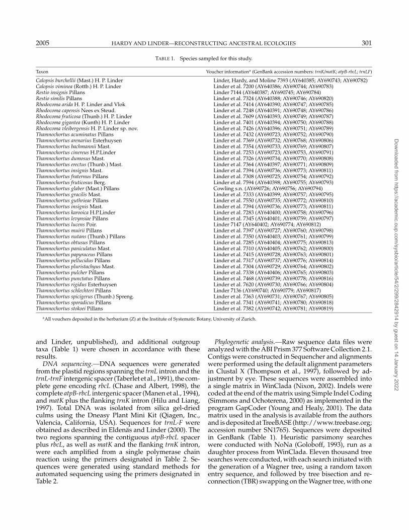
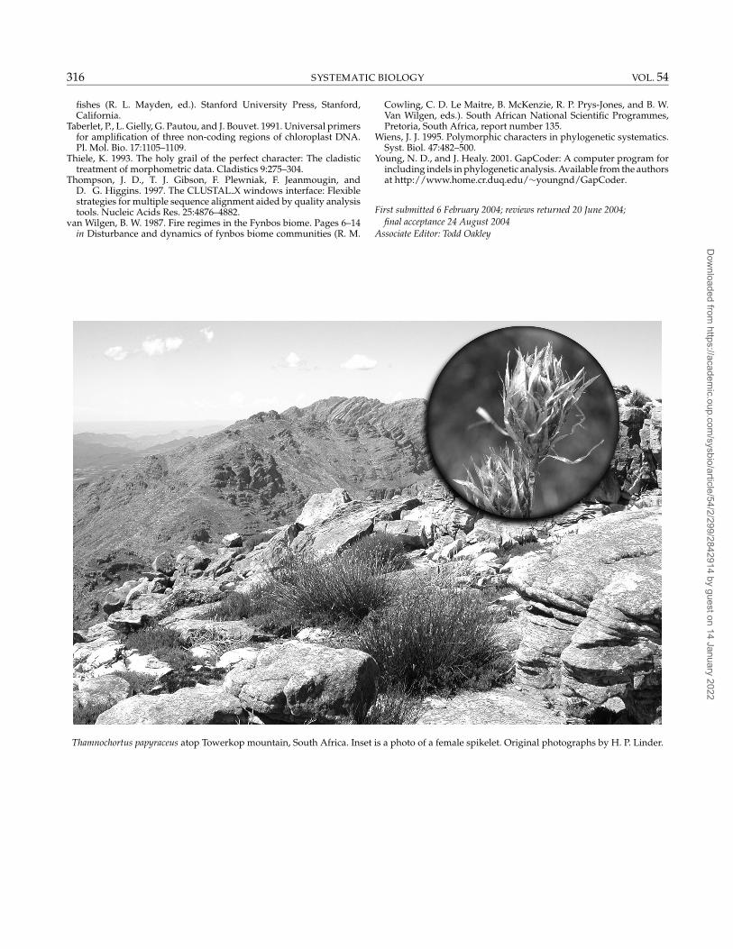
Thamnochortus papyraceus atop Towerkop mountain, South Africa. Inset is a photo of a female spikelet. Original photographs by H. P. Linder.

Cowling, C. D. Le Maitre, B. McKenzie, R. P. Prys-Jones, and B. W.Van Wilgen, eds.). South African National Scientific Programmes,Pretoria, South Africa, report number 135.

Wiens, J. J. 1995. Polymorphic characters in phylogenetic systematics.Syst. Biol. 47:482–500.

Young, N. D., and J. Healy. 2001. GapCoder: A computer program forincluding indels in phylogenetic analysis. Available from the authorsat http://www.home.cr.duq.edu/∼youngnd/GapCoder.

First submitted 6 February 2004; reviews returned 20 June 2004;final acceptance 24 August 2004

Associate Editor: Todd Oakley

Dow



Documents

Intraspecific Variability and Timing in Ancestral Ecology