Finance and Economics Discussion SeriesDivisions of Research & Statistics and Monetary Affairs

Federal Reserve Board, Washington, D.C.

The Role of Learning for Asset Prices, Business Cycles, andMonetary Policy

Fabian Winkler

2016-019

Please cite this paper as:Winkler, Fabian (2016). “The Role of Learning for Asset Prices, Business Cycles, andMonetary Policy,” Finance and Economics Discussion Series 2016-019. Washington: Boardof Governors of the Federal Reserve System, http://dx.doi.org/10.17016/FEDS.2016.019.

NOTE: Staff working papers in the Finance and Economics Discussion Series (FEDS) are preliminarymaterials circulated to stimulate discussion and critical comment. The analysis and conclusions set forthare those of the authors and do not indicate concurrence by other members of the research staff or theBoard of Governors. References in publications to the Finance and Economics Discussion Series (other thanacknowledgement) should be cleared with the author(s) to protect the tentative character of these papers.

The Role of Learning for Asset Prices, Business Cycles, andMonetary Policy

Fabian Winkler∗

20 January 2016

Abstract

The importance of financial frictions for the business cycle is widely recognized, but it is lessrecognized that their effects depend heavily on the underlying asset pricing theory. This paperexamines the implications of learning-based asset pricing. I construct a model in which firms’ability to access credit depends on their market value, and investors rely on past observationto predict future stock prices. Agents’ expectations remain model-consistent conditional ontheir beliefs about stock prices, which disciplines the expectation formation process. The modelmatches several asset price properties such as return volatility and predictability and also leadsto a powerful feedback loop between asset prices and real activity, substantially amplifyingbusiness cycle shocks. Agents’ expectational errors on asset prices spill over to forecasts ofeconomic activity, resulting in forecast error predictability that closely matches survey data. Areaction of monetary policy to asset prices is welfare-improving under learning but not underrational expectations.

Keywords: Learning, Asset Pricing, Credit Constraints, Monetary Policy, Survey DataJEL Classification: D83, E32, E44, E52, G12

∗Board of Governors of the Federal Reserve System, 20th St and Constitution Ave NW, Washington DC 20551,fabian.winkler@frb.gov. I thank Wouter den Haan for his guidance and support; Klaus Adam, Andrea Ajello, Jo-hannes Boehm, Peter Karadi, Albert Marcet, Stéphane Moyen, Rachel Ngai, Markus Riegler, and participants at theECB-CFS-Bundesbank lunchtime seminar, Singapore Management University, Econometric Society Winter Meetingin Madrid, EEA Annual Meeting in Toulouse, and Econometric Society World Congress in Montreal, for useful com-ments and suggestions. The views herein are those of the author and do not represent the views of the Board ofGovernors of the Federal Reserve System or the Federal Reserve System.

1 Introduction

I think financial factors in general, and asset prices in particular, play a more central role inexplaining the dynamics of the economy than is typically reflected in macro-economic models,even after the experience of the crisis.— Andrew Haldane, Chief Economist of the Bank of England, 30 April 2014

The above statement may provoke disbelief among macroeconomists. After all, a wealth of researchin the last 15 years has been dedicated precisely to the links between the financial sector and thereal economy. Financial frictions are now seen as a central mechanism by which asset prices interactwith macroeconomic dynamics. Yet our understanding of this interaction remains incomplete, inpart due to the inherent difficulty of modelling asset prices.

Typical business cycle models still rely on an asset pricing theory based on rational expectations,time-separable preferences and moderate degrees of risk aversion. It is well known that such anasset pricing theory is inadequate for many empirical asset price regularities, which have thereforebeen named “puzzles”. Some of the most famous such puzzles are that prices are volatile (Shiller,1981), returns are predictable at business cycle frequency (Fama and French, 1988), and exhibitnegative skewness and excess kurtosis (Campbell and Hentschel, 1992).1At the same time, assetprices play a central role in the real economy in the presence of financial frictions. Conclusionsdrawn from models with financial frictions but without a good asset pricing theory are thereforequestionable.

There is not a shortage of theories that aim to explain asset prices. Most of them keep the rationalexpectations assumption and engineer preferences that deliver highly volatile discount factors. Thedominant approaches are based on non-linear habit formation (Campbell and Cochrane, 1999) orEpstein-Zin preferences together with “long-run risk” (Bansal and Yaron, 2004). There are howevercompelling arguments for relaxing the rational expectations assumption instead. Measurements ofexpectations in surveys do not support the notion that agents have rational expectations. Ra-tional expectations imply, for example, that investors are fully aware of return predictability inthe stock market, expecting lower returns when prices are high and vice versa. Instead, measuredexpectations imply they expect higher returns. This pattern has been documented extensively byGreenwood and Shleifer (2014) and is illustrated in Figure 1. The left panel plots the mean 12-month return expectation of the S&P500, as measured in the Graham-Harvey survey of AmericanCFOs, against the value of the P/D ratio in the month preceding the survey. The correlation isstrongly positive: Return expectations are more optimistic when stock valuations are high. How-ever, high stock valuations actually predict low future returns of the S&P500, as documented aboveand illustrated again in the right panel of the figure. Unless one rejects surveys as an unbiasedmeasure of expectations, such a pattern cannot be reconciled with rational expectations.

1Another such puzzle is the size of the equity premium. Adam, Marcet, and Nicolini (2015) show that learningmodels similar to the one in this paper are able to generate a sizable equity premium, but it is not the subject of thispaper.

1

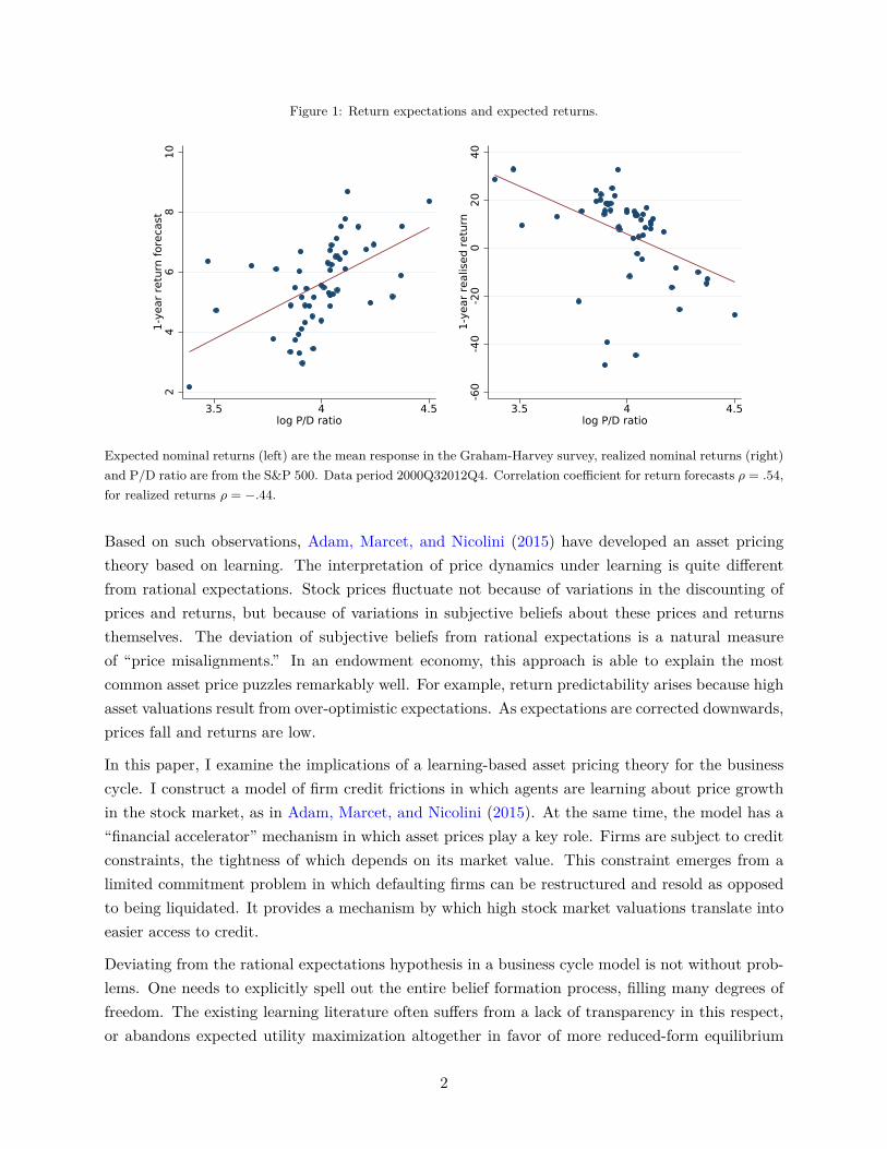
Figure 1: Return expectations and expected returns.

24

68

101-

year

ret

urn

fore

cast

3.5 4 4.5log P/D ratio

-60

-40

-20

020

401-

year

rea

lised

ret

urn

3.5 4 4.5log P/D ratio

Expected nominal returns (left) are the mean response in the Graham-Harvey survey, realized nominal returns (right)and P/D ratio are from the S&P 500. Data period 2000Q32012Q4. Correlation coefficient for return forecasts ρ = .54,for realized returns ρ = −.44.

Based on such observations, Adam, Marcet, and Nicolini (2015) have developed an asset pricingtheory based on learning. The interpretation of price dynamics under learning is quite differentfrom rational expectations. Stock prices fluctuate not because of variations in the discounting ofprices and returns, but because of variations in subjective beliefs about these prices and returnsthemselves. The deviation of subjective beliefs from rational expectations is a natural measureof “price misalignments.” In an endowment economy, this approach is able to explain the mostcommon asset price puzzles remarkably well. For example, return predictability arises because highasset valuations result from over-optimistic expectations. As expectations are corrected downwards,prices fall and returns are low.

In this paper, I examine the implications of a learning-based asset pricing theory for the businesscycle. I construct a model of firm credit frictions in which agents are learning about price growthin the stock market, as in Adam, Marcet, and Nicolini (2015). At the same time, the model has a“financial accelerator” mechanism in which asset prices play a key role. Firms are subject to creditconstraints, the tightness of which depends on its market value. This constraint emerges from alimited commitment problem in which defaulting firms can be restructured and resold as opposedto being liquidated. It provides a mechanism by which high stock market valuations translate intoeasier access to credit.

Deviating from the rational expectations hypothesis in a business cycle model is not without prob-lems. One needs to explicitly spell out the entire belief formation process, filling many degrees offreedom. The existing learning literature often suffers from a lack of transparency in this respect,or abandons expected utility maximization altogether in favor of more reduced-form equilibrium

2

conditions. To address this problem, I develop an expectation concept that I call “conditionallymodel-consistent expectations.” This can be seen as a refinement of the “internal rationality” re-quirement developed by Adam and Marcet (2011). Agents continue to maximize a well-definedstable objective function with coherent and time-consistent beliefs about the variables affectingtheir decisions. They can entertain arbitrary beliefs about one relative price in the economy, whichwill be the price of stocks in this paper. But their beliefs about any other variable must be consis-tent with the equilibrium conditions of the model, except for market clearing in the stock market(and one more market, owing to Walras’ law). This implies that when agents endowed with theseexpectations evaluate their forecast errors, they find that their forecasting rules cannot be improvedupon conditional on their subjective belief about stock prices. In this sense this is a minimal de-parture from rational expectations. What’s more, spelling out a belief system for stock prices andthen imposing conditionally model-consistent expectations is all that is needed to obtain a uniquedynamic equilibrium. This allows me to transparently incorporate asset price learning into anybusiness cycle model while introducing only one additional parameter and one state variable.

The analysis of the model yields three results. First, a positive feedback loop emerges betweenasset prices and the production side of the economy, which leads to considerable amplification andpropagation of business cycle shocks. When investor beliefs are more optimistic, their demand forstocks increases. This raises firm valuations and relaxes credit condition, in turn allowing firmsto move closer to their profit optimum. If countervailing general equilibrium forces are not toostrong, firms will be able to pay higher dividends to their shareholders, raising stock prices furtherand propagating investor optimism. The financial accelerator mechanism becomes quantitativelymore important than under rational expectations. At the same time, learning greatly improvesasset price properties such as price and return volatility and predictability. This result suggeststhat the relatively weak quantitative strength of the financial accelerator effect in many existingmodels—as discussed in (Cordoba and Ripoll, 2004)—is at least in part due to low endogenousasset price volatility.

Second, I compare the forecasts of agents in the model with actual forecasts in survey data, for bothasset prices and real quantities. Even though agents only learn about stock prices in the model,their expectational errors spill over into their forecasts of other variables. For example, when agentsare too optimistic about asset prices, they also become too optimistic about the tightness of creditconstraints and therefore over-predict future investment. I find that the replicates remarkably wellthe predictability of forecast errors by forecast revisions as in Coibion and Gorodnichenko (2015),as well as by the level and growth rate of the price-dividend ratio. This lends credibility to thechoice of the expectation formation process.

Third, I show that the model has important normative implications. A recurring question inmonetary economics is whether policy should react to asset price “misalignments”; or “lean againstthe wind.” Gali (2014) writes that justifying such a reaction requires “the presumption that anincrease in interest rates will reduce the size of an asset price bubble,” for which “no empirical ortheoretical support seems to have been provided.” This paper is a first step towards filling this

3

gap. Indeed, I find that under learning, the welfare-maximizing monetary interest rate rule reactsstrongly to asset price growth. By raising interest rates when stock prices are rising, policy isable to curb the endogenous build-up of over-optimistic investor beliefs, reducing both asset priceand business cycle volatility. In contrast, under rational expectations, adding a policy reaction toasset prices carries no welfare benefits, in line with earlier findings in the literature (Bernanke andGertler, 2001; Faia and Monacelli, 2007). The result highlights the importance of expectations infinancial markets for normative questions.

There is a large literature studying the effect of asset prices on business cycle fluctuations, whichrelates to this paper. In particular, Xu, Wang, and Miao (2013) develop a model in which borrowinglimits depend on stock market valuations through a credit friction similar to that in my model.They prove the existence of rational liquidity bubbles and introduce a shock that governs the sizeof this bubble, thus allowing them to exactly match the stock prices seen in the data. Other studies(e.g. Iacoviello, 2005; Liu, Wang, and Zha, 2013) similarly “explain” asset price fluctuations bydirect shocks to prices in order to study the effects of financial frictions. In this paper, asset pricevolatility is not driven by an additional shock but instead an endogenous outcome of the learningdynamics.

There are some studies that endogenize asset price dynamics in production economies with rationalexpectations. They make use of habit formation (Boldrin, Christiano, and Fisher, 2001) or long-runrisk (Tallarini Jr., 2000; Croce, 2014). The goal there is to replicate both standard asset price andbusiness cycle moments within a close variant of the real business cycle model. This turns outto be a difficult task because the complex preferences in these models have some counterfactualimplications (Lettau and Uhlig, 2000; Epstein, Farhi, and Strzalecki, 2013); to my knowledge, theseasset price theories have not been applied to more elaborate business cycle models. The modelin this paper can be solved conveniently in the presence of such frictions using a perturbationapproach. Moreover, the inefficient nature of price fluctuations leads to policy implications thatare quite different from an efficient markets world.

This paper also contributes to the literature on learning in business cycle models. A number ofpapers in this area have studied learning in combination with financial frictions (Caputo, Medina,and Soto, 2010; Milani, 2011; Gelain, Lansing, and Mendicino, 2013). The approach consistsof two steps: first, derive the linearized equilibrium conditions of the economy under rationalexpectations; second, replace all terms involving expectations with parameterized forecast functions,and update the parameters using recursive least squares every period. Such models certainlyproduce very rich dynamics, but they are problematic on several grounds. First, such parameterizedexpectation equations often do not correspond anymore to intertemporal optimization problems.Second, analysis of these models is often complex and lack transparency due to the large numberof parameters and state variables involved. Here, I develop a more transparent and parsimoniousapproach. Beliefs are restricted to be conditionally model-consistent and agents make optimalchoices given a consistent set of beliefs, preserving much of the intuition of a rational expectationsmodel.

4

The remainder of the paper is structured as follows. Section 2 presents a simplified version of themodel that permits an analytic solution. It shows that credit frictions or asset price learning alonedoes not generate either amplification of shocks or interesting asset price dynamics, although theircombination does. The full model is presented in Section 3. Section 4 contains the quantitativeresults. Section 5 contains sensitivity checks. Section 6 discusses monetary policy implications.Section 7 concludes.

2 Simplified model

In this section, I construct a simplified version of the model which illustrates the interaction betweencredit frictions and learning about asset prices. The model allows for a closed-form solution, butquantitative analysis will require extending it in the next section. The key insight here is thatfinancial frictions alone do not generate sizable amplification of business cycle shocks or asset pricevolatility, while in combination with learning they do.

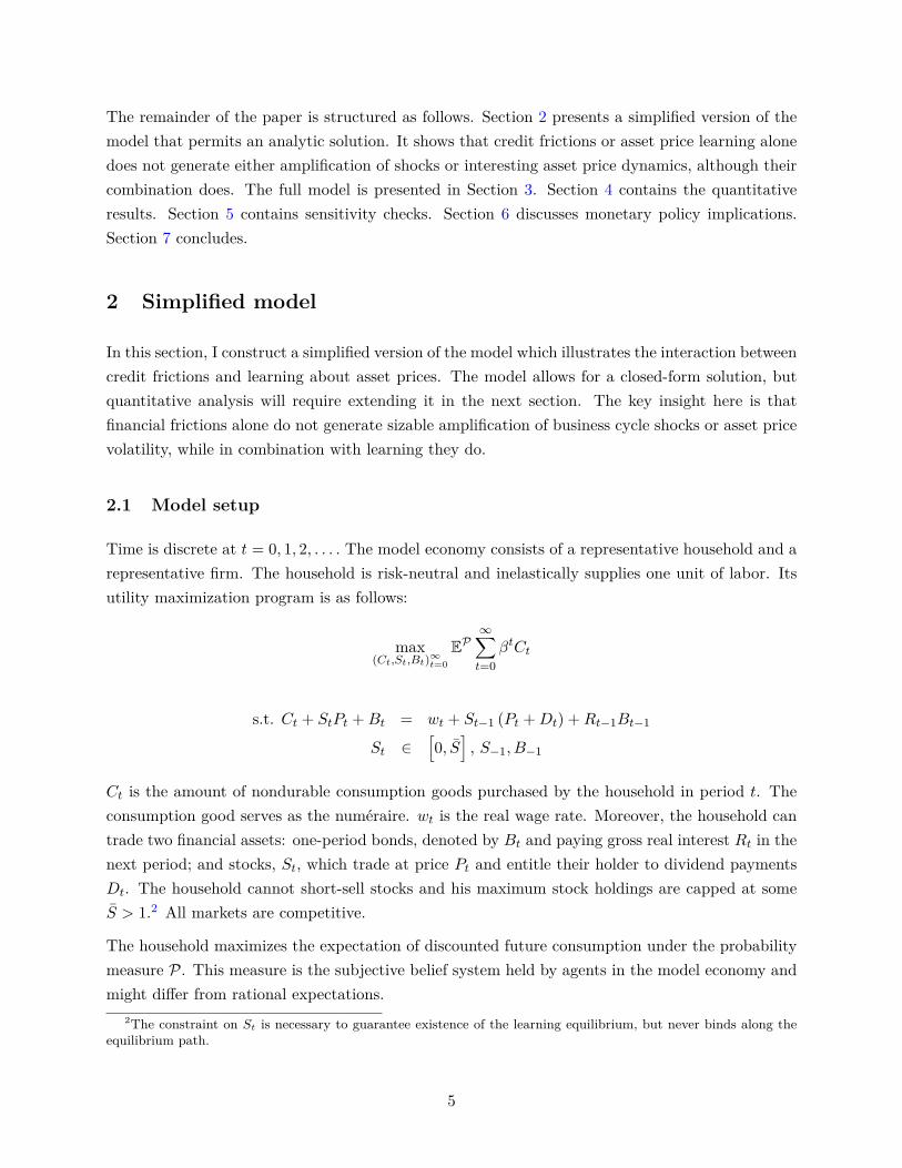
2.1 Model setup

Time is discrete at t = 0, 1, 2, . . . . The model economy consists of a representative household and arepresentative firm. The household is risk-neutral and inelastically supplies one unit of labor. Itsutility maximization program is as follows:

max(Ct,St,Bt)∞t=0

EP∞∑t=0

βtCt

s.t. Ct + StPt +Bt = wt + St−1 (Pt +Dt) +Rt−1Bt−1

St ∈[0, S

], S−1, B−1

Ct is the amount of nondurable consumption goods purchased by the household in period t. Theconsumption good serves as the numéraire. wt is the real wage rate. Moreover, the household cantrade two financial assets: one-period bonds, denoted by Bt and paying gross real interest Rt in thenext period; and stocks, St, which trade at price Pt and entitle their holder to dividend paymentsDt. The household cannot short-sell stocks and his maximum stock holdings are capped at someS > 1.2 All markets are competitive.

The household maximizes the expectation of discounted future consumption under the probabilitymeasure P. This measure is the subjective belief system held by agents in the model economy andmight differ from rational expectations.

2The constraint on St is necessary to guarantee existence of the learning equilibrium, but never binds along theequilibrium path.

5

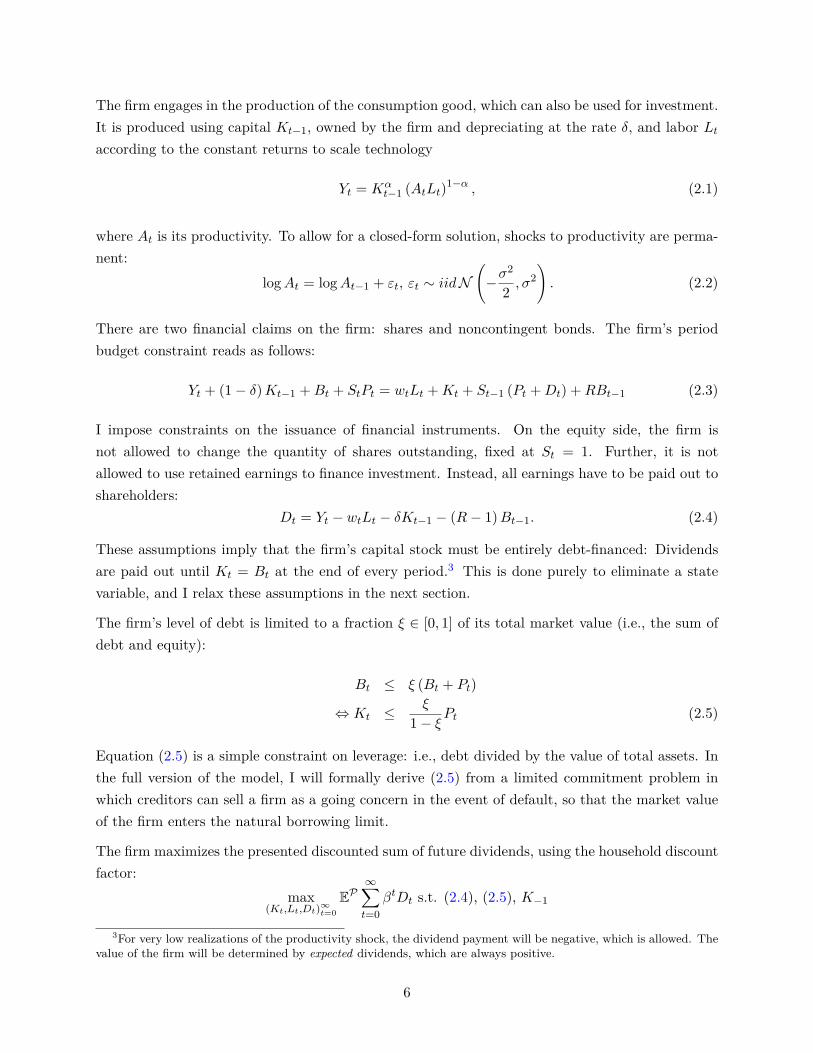
The firm engages in the production of the consumption good, which can also be used for investment.It is produced using capital Kt−1, owned by the firm and depreciating at the rate δ, and labor Ltaccording to the constant returns to scale technology

Yt = Kαt−1 (AtLt)1−α , (2.1)

where At is its productivity. To allow for a closed-form solution, shocks to productivity are perma-nent:

logAt = logAt−1 + εt, εt ∼ iidN(−σ

2

2 , σ2). (2.2)

There are two financial claims on the firm: shares and noncontingent bonds. The firm’s periodbudget constraint reads as follows:

Yt + (1− δ)Kt−1 +Bt + StPt = wtLt +Kt + St−1 (Pt +Dt) +RBt−1 (2.3)

I impose constraints on the issuance of financial instruments. On the equity side, the firm isnot allowed to change the quantity of shares outstanding, fixed at St = 1. Further, it is notallowed to use retained earnings to finance investment. Instead, all earnings have to be paid out toshareholders:

Dt = Yt − wtLt − δKt−1 − (R− 1)Bt−1. (2.4)

These assumptions imply that the firm’s capital stock must be entirely debt-financed: Dividendsare paid out until Kt = Bt at the end of every period.3 This is done purely to eliminate a statevariable, and I relax these assumptions in the next section.

The firm’s level of debt is limited to a fraction ξ ∈ [0, 1] of its total market value (i.e., the sum ofdebt and equity):

Bt ≤ ξ (Bt + Pt)

⇔ Kt ≤ξ

1− ξPt (2.5)

Equation (2.5) is a simple constraint on leverage: i.e., debt divided by the value of total assets. Inthe full version of the model, I will formally derive (2.5) from a limited commitment problem inwhich creditors can sell a firm as a going concern in the event of default, so that the market valueof the firm enters the natural borrowing limit.

The firm maximizes the presented discounted sum of future dividends, using the household discountfactor:

max(Kt,Lt,Dt)∞t=0

EP∞∑t=0

βtDt s.t. (2.4), (2.5), K−1

3For very low realizations of the productivity shock, the dividend payment will be negative, which is allowed. Thevalue of the firm will be determined by expected dividends, which are always positive.

6

In particular, it makes its decisions under the same belief system P as the household—expectationsare homogenous.

The model is closed by specifying market clearing conditions for the goods, labor and equity mar-kets:

Yt +Kt = C + (1− δ)Kt−1 (2.6)

Lt = 1 (2.7)

St = 1. (2.8)

An equilibrium for an arbitrary subjective probability measure P is defined as a mapping from real-izations of the exogenous variable (At)∞t=0 and initial conditions (B−1,K−1, R−1) to the endogenousvariables (Bt,Kt, Lt, Dt, Pt, Rt, wt, Ct, St)∞t=0 such that markets clear and agents’ choices solve theiroptimization problem under the probability measure P. In particular, the first order conditions ofthe household and firm must hold at all times.4

The first-order conditions describing the household’s optimal plan are Rt = R = β−1 for bonds and

St

= 0 if Pt > βEPt [Pt+1 +Dt+1]

∈[0, S

]if Pt = βEPt [Pt+1 +Dt+1]

= S if Pt < βEPt [Pt+1 +Dt+1]

(2.9)

for stocks. In a rational expectations setup, one would quickly substitute the market clearingcondition St = 1 and write (2.9) as an equality. However, this already assumes that agents knowhow many outstanding shares they will hold in equilibrium. Under learning, they will not beendowed with this knowledge.

The firm’s optimal labor demand and constraints imply the following expression for dividends:

Dt =(Rkt −Rt−1

)Kt−1, (2.10)

where the marginal return on capital is

Rkt = α

((1− α) At

wt

) 1−αα

+ 1− δ. (2.11)

When choosing the optimal amount of capital then, the firm exhausts its borrowing limit as long4This definition satisfies the “internal rationality” requirement of Adam and Marcet (2011).

7

as the expected internal return on capital exceeds the external return paid to creditors:

Kt

= 0 if EPt Rkt+1 < Rt

∈[0, ξ

1−ξPt]

if EPt Rkt+1 = Rt

= ξ1−ξPt if EPt Rkt+1 > Rt.

(2.12)

These optimality conditions must hold under any belief P used to form expectations.

2.2 Rational expectations equilibrium

I first describe the equilibrium under rational expectations. Rational expectations amount to aparticular choice of the measure P. This measure has to coincide with the measure induced by theequilibrium allocations. In that case, one writes EP [·] = E [·].

The equilibrium under rational expectations admits a closed-form solution. First, let us considerthe case ξ = 1. In this case, the borrowing constraint (2.5) can never bind. Capital is therefore atits efficient level, which is simply proportional to productivity: Kt = K∗At such that EtRkt+1 = R.Expected dividends and the market value of equity are zero: EtDt+1 = 0 and Pt = 0. Intuitively,when the firm is unconstrained, the expected return on capital must equal the interest rate onborrowing, and since all capital is financed by debt and the production function has constantreturns to scale, in expectation all profits are paid out as interest payments to debt holders. Theresidual equity claims trade at a price of zero.

Once we introduce financial frictions by setting ξ < 1, how much amplification do we get? Theanswer is: none. Now the equilibrium is characterized by two equations:

PtAt

= P =exp

(−α(1−α)

2 σ2)αKα − (R− 1 + δ) KR

(2.13)

Kt

At= K = ξ

1− ξ P (2.14)

The first equation pins down the stock market value of the firm as a function of the capital stock.The second equation determines the capital stock that can be reached by exhausting the borrowingconstraint that depends on the stock market value. In particular, the borrowing constraint isalways binding. In equilibrium, the equilibrium capital stock and stock price comove perfectly withproductivity, just as in the case of ξ = 1. Financial frictions do not lead to any amplification orpropagation of shocks in the rational expectations equilibrium. They have a level effect on output,capital, etc., but the dynamics of the model are identical for any value of ξ. The variances oflog stock price and output growth do not depend on ξ and are bounded by the variance of the

8

exogenous shock σ2:

Var [∆ logPt] = σ2 (2.15)

Var [∆ log Yt] =(1− 2α+ 2α2

)σ2 (2.16)

Intuitively, with financial frictions, a shock to productivity raises asset prices just as much as toallow the firm to instantly adjust the capital stock proportionately. At the same time, stock returnsare not volatile and unpredictable at all horizons.

Before moving on to the learning equilibrium, it is worth noting that the stock price and thedividend payment of the firm are non-monotonic in the level of financial frictions ξ:

Et [Dt+1] = D (kt,Kt, At) =(Etα

(At+1Kt

)1−α+ 1− δ −R

)kt. (2.17)

Here, I have made a distinction between the capital choice kt of the firm that takes future wagesas given, and the aggregate capital stock Kt, which determines wages and the return on capital ingeneral equilibrium. Of course, in equilibrium the two are equal. When ξ = 0, the firm cannotborrow at all and kt = 0, and when ξ = 1 we have EtRkt+1 = R. In both cases, expected dividendsand the value of the firm are zero. In between these extreme cases, there are two opposing forcesaffecting expected dividends:

d

dξD(K, K, At

)=

∂D∂k (kt,Kt, At)︸ ︷︷ ︸>0

+ ∂D

∂K(kt,Kt, At)︸ ︷︷ ︸<0

dKdξ︸︷︷︸>0

. (2.18)

The first term in brackets captures a partial equilibrium effect of leverage, which is internalizedby the firm. When a firm is financially constrained, its internal rate of return is higher than thereturn it has to pay to debt holders. It will then want to increase its capital stock by borrowinguntil it reachtes the borrowing constraint, thereby increasing expected dividends. The second termcaptures a general equilibrium effect: Higher investment lowers the marginal product of capital,which in practice is realized through an increase in the equilibrium wage wt+1, reducing expecteddividends. When ξ is small (financial frictions are severe) the partial equilibrium effect dominates,while for a large ξ, the general equilibrium effect dominates.

2.3 Learning equilibrium

I now introduce learning about stock prices by changing the subjective probability measure P.Learning will increase the volatility of stock prices, account for return and forecast error predictabil-ity, and, most importantly, induce endogenous amplification and propagation on the productionside of the model in combination with financial frictions.

9

The only departure from rational expectations is that agents do not understand the pricing func-tion that maps fundamentals into an equilibrium stock price. Agents are not endowed with theknowledge that prices obey the market-clearing condition:

Pt = βEPt [Pt+1 +Dt+1] . (2.19)

Instead, they form subjective beliefs about the law of motion of prices and update them usingrealized price observations. I impose the following restrictions on these beliefs. Under the subjectivemeasure P,

1. agents have the correct belief about the fundamental At;

2. agents believe that the stock price Pt evolves according to

logPt − logPt−1 = µt + ηt (2.20)

µt = µt−1 + νt (2.21)

where(ηt

νt

)∼ N

(−1

2

(σ2η

σ2ν

),

(σ2η 0

0 σ2ν

))iid, (2.22)

the variable µt and the disturbances ηt and νt are unobserved and the prior about µt in period0 is given by

µ0 | F0 ∼ N(µ0, σ

2µ

)where σ2

µ =−σ2

ν +√σ4ν + 4σ2

νσ2η

2 ; (2.23)

3. agents update their beliefs about µt after making their choices and observing equilibriumprices in period t;

4. for any variable xt relevant for agents’ decision problems and t ≥ 0, agents’ beliefs coincidewith model outcomes on the equilibrium path, conditional on the realization of stock pricesand fundamentals:

EP [xt | A0, . . . , At, P0, . . . , Pt] = xt.

The first assumption implies that agents have as much information about the fundamental shocksof the economy as under rational expectations. The second assumption amounts to saying thatagents believe stock prices to be a random walk. This random walk is believed to have a small,unobservable, and time-varying drift µt. Learning about this drift is going to be the key driverof asset price dynamics. The third assumption imposes that forecasts of stock prices are updatedafter equilibrium prices are determined.5Together, (2.20)–(2.23) form a linear state-space system.Under P, agents’ beliefs about µt at time t are normally distributed with stationary variance σ2

µ

5This “lagged belief updating” is common in the learning literature. It makes all feedback between forecasts andprices inter- rather than intratemporal. For further discussion see Adam, Beutel, and Marcet (2014).

10

and mean µt−1, which evolves according to the Kalman filtering equation:

µt = µt−1 −σ2ν

2 + g

(logPt − logPt−1 +

σ2η + σ2

ν

2 − µt−1

)(2.24)

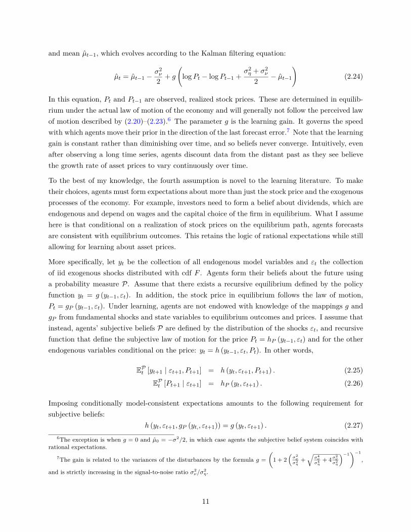
In this equation, Pt and Pt−1 are observed, realized stock prices. These are determined in equilib-rium under the actual law of motion of the economy and will generally not follow the perceived lawof motion described by (2.20)–(2.23).6 The parameter g is the learning gain. It governs the speedwith which agents move their prior in the direction of the last forecast error.7 Note that the learninggain is constant rather than diminishing over time, and so beliefs never converge. Intuitively, evenafter observing a long time series, agents discount data from the distant past as they see believethe growth rate of asset prices to vary continuously over time.

To the best of my knowledge, the fourth assumption is novel to the learning literature. To maketheir choices, agents must form expectations about more than just the stock price and the exogenousprocesses of the economy. For example, investors need to form a belief about dividends, which areendogenous and depend on wages and the capital choice of the firm in equilibrium. What I assumehere is that conditional on a realization of stock prices on the equilibrium path, agents forecastsare consistent with equilibrium outcomes. This retains the logic of rational expectations while stillallowing for learning about asset prices.

More specifically, let yt be the collection of all endogenous model variables and εt the collectionof iid exogenous shocks distributed with cdf F . Agents form their beliefs about the future usinga probability measure P. Assume that there exists a recursive equilibrium defined by the policyfunction yt = g (yt−1, εt). In addition, the stock price in equilibrium follows the law of motion,Pt = gP (yt−1, εt). Under learning, agents are not endowed with knowledge of the mappings g andgP from fundamental shocks and state variables to equilibrium outcomes and prices. I assume thatinstead, agents’ subjective beliefs P are defined by the distribution of the shocks εt, and recursivefunction that define the subjective law of motion for the price Pt = hP (yt−1, εt) and for the otherendogenous variables conditional on the price: yt = h (yt−1, εt, Pt). In other words,

EPt [yt+1 | εt+1, Pt+1] = h (yt, εt+1, Pt+1) . (2.25)

EPt [Pt+1 | εt+1] = hP (yt, εt+1) . (2.26)

Imposing conditionally model-consistent expectations amounts to the following requirement forsubjective beliefs:

h (yt, εt+1, gP (yt,, εt+1)) = g (yt, εt+1) . (2.27)6The exception is when g = 0 and µ0 = −σ2/2, in which case agents the subjective belief system coincides with

rational expectations.7The gain is related to the variances of the disturbances by the formula g =

(1 + 2

(σ2ν

σ2η

+√

σ4ν

σ4η

+ 4σ2ν

σ2η

)−1)−1

,

and is strictly increasing in the signal-to-noise ratio σ2ν/σ

2η.

11

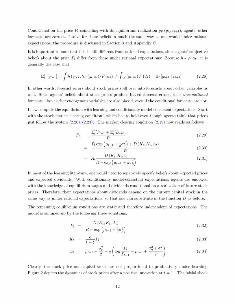
Conditional on the price Pt coinciding with its equilibrium realization gP (yt,, εt+1), agents’ otherforecasts are correct. I solve for these beliefs in much the same way as one would under rationalexpectations; the procedure is discussed in Section 3 and Appendix C.

It is important to note that this is still different from rational expectations, since agents’ subjectivebeliefs about the price Pt differ from those under rational expectations: Because hP 6= gP , it isgenerally the case that

EPt [yt+1] =ˆh (yt, ε, hP (yt, εt))F (dε) 6=

ˆg (yt, εt)F (dε) = Et [yt+1 | εt+1] . (2.28)

In other words, forecast errors about stock prices spill over into forecasts about other variables aswell. Since agents’ beliefs about stock prices produce biased forecast errors, their unconditionalforecasts about other endogenous variables are also biased, even if the conditional forecasts are not.

I now compute the equilibrium with learning and conditionally model-consistent expectations. Startwith the stock market clearing condition , which has to hold even though agents think that pricesjust follow the system (2.20)–(2.23)). The market clearing condition (2.19) now reads as follows:

Pt = EPt Pt+1 + EPt Dt+1R

(2.29)

=Pt exp

(µt−1 + 1

2σ2µ

)+D (Kt,Kt, At)

R(2.30)

= AtD (Kt,Kt, 1)

R− exp(µt−1 + 1

2σ2µ

) (2.31)

In most of the learning literature, one would need to separately specify beliefs about expected pricesand expected dividends. With conditionally model-consistent expectations, agents are endowedwith the knowledge of equilibrium wages and dividends conditional on a realization of future stockprices. Therefore, their expectations about dividends depend on the current capital stock in thesame way as under rational expectations, so that one can substitute in the function D as before.

The remaining equilibrium conditions are static and therefore independent of expectations. Themodel is summed up by the following three equations:

Pt = D (Kt,Kt, At)R− exp

(µt−1 + 1

2σ2µ

) (2.32)

Kt = ξ

1− ξPt (2.33)

µt = µt−1 −σ2ν

2 + g

(log Pt

Pt−1− µt−1 +

σ2η + σ2

ν

2

)(2.34)

Clearly, the stock price and capital stock are not proportional to productivity under learning.Figure 2 depicts the dynamics of stock prices after a positive innovation at t = 1 . The initial shock

12

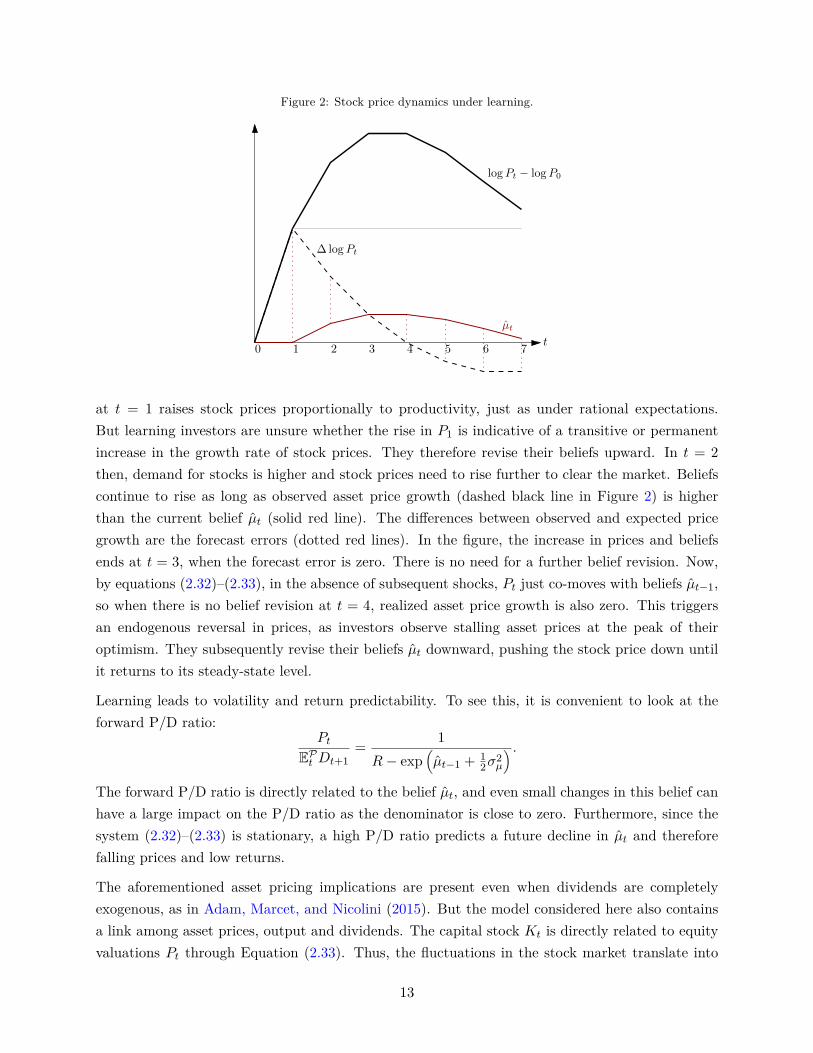
Figure 2: Stock price dynamics under learning.

t

logPt − logP0

∆ logPt

µt

0 1 2 3 4 5 6 7

at t = 1 raises stock prices proportionally to productivity, just as under rational expectations.But learning investors are unsure whether the rise in P1 is indicative of a transitive or permanentincrease in the growth rate of stock prices. They therefore revise their beliefs upward. In t = 2then, demand for stocks is higher and stock prices need to rise further to clear the market. Beliefscontinue to rise as long as observed asset price growth (dashed black line in Figure 2) is higherthan the current belief µt (solid red line). The differences between observed and expected pricegrowth are the forecast errors (dotted red lines). In the figure, the increase in prices and beliefsends at t = 3, when the forecast error is zero. There is no need for a further belief revision. Now,by equations (2.32)–(2.33), in the absence of subsequent shocks, Pt just co-moves with beliefs µt−1,so when there is no belief revision at t = 4, realized asset price growth is also zero. This triggersan endogenous reversal in prices, as investors observe stalling asset prices at the peak of theiroptimism. They subsequently revise their beliefs µt downward, pushing the stock price down untilit returns to its steady-state level.

Learning leads to volatility and return predictability. To see this, it is convenient to look at theforward P/D ratio:

PtEPt Dt+1

= 1R− exp

(µt−1 + 1

2σ2µ

) .The forward P/D ratio is directly related to the belief µt, and even small changes in this belief canhave a large impact on the P/D ratio as the denominator is close to zero. Furthermore, since thesystem (2.32)–(2.33) is stationary, a high P/D ratio predicts a future decline in µt and thereforefalling prices and low returns.

The aforementioned asset pricing implications are present even when dividends are completelyexogenous, as in Adam, Marcet, and Nicolini (2015). But the model considered here also containsa link among asset prices, output and dividends. The capital stock Kt is directly related to equityvaluations Pt through Equation (2.33). Thus, the fluctuations in the stock market translate into

13

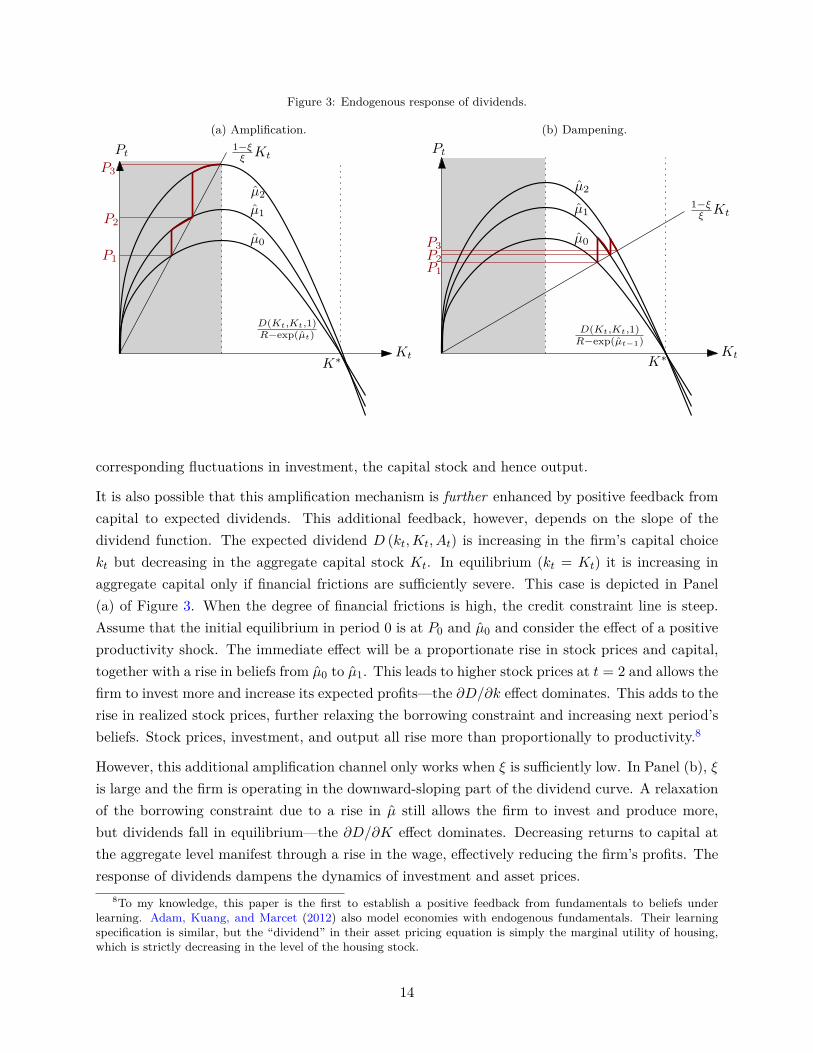
Figure 3: Endogenous response of dividends.

(a) Amplification.

Kt

1−ξξ

Kt

D(Kt;Kt;1)R−exp(µt)

µ0

µ1

µ2

K∗

P1

P2

P3

Pt

(b) Dampening.

Kt

1−ξξ

Kt

D(Kt;Kt;1)R−exp(µt−1)

µ0

µ1

µ2

K∗

P1

P2

P3

Pt

corresponding fluctuations in investment, the capital stock and hence output.

It is also possible that this amplification mechanism is further enhanced by positive feedback fromcapital to expected dividends. This additional feedback, however, depends on the slope of thedividend function. The expected dividend D (kt,Kt, At) is increasing in the firm’s capital choicekt but decreasing in the aggregate capital stock Kt. In equilibrium (kt = Kt) it is increasing inaggregate capital only if financial frictions are sufficiently severe. This case is depicted in Panel(a) of Figure 3. When the degree of financial frictions is high, the credit constraint line is steep.Assume that the initial equilibrium in period 0 is at P0 and µ0 and consider the effect of a positiveproductivity shock. The immediate effect will be a proportionate rise in stock prices and capital,together with a rise in beliefs from µ0 to µ1. This leads to higher stock prices at t = 2 and allows thefirm to invest more and increase its expected profits—the ∂D/∂k effect dominates. This adds to therise in realized stock prices, further relaxing the borrowing constraint and increasing next period’sbeliefs. Stock prices, investment, and output all rise more than proportionally to productivity.8

However, this additional amplification channel only works when ξ is sufficiently low. In Panel (b), ξis large and the firm is operating in the downward-sloping part of the dividend curve. A relaxationof the borrowing constraint due to a rise in µ still allows the firm to invest and produce more,but dividends fall in equilibrium—the ∂D/∂K effect dominates. Decreasing returns to capital atthe aggregate level manifest through a rise in the wage, effectively reducing the firm’s profits. Theresponse of dividends dampens the dynamics of investment and asset prices.

8To my knowledge, this paper is the first to establish a positive feedback from fundamentals to beliefs underlearning. Adam, Kuang, and Marcet (2012) also model economies with endogenous fundamentals. Their learningspecification is similar, but the “dividend” in their asset pricing equation is simply the marginal utility of housing,which is strictly decreasing in the level of the housing stock.

14

I end this section with the observation that the equilibrium dynamics are driven by the interactionof financial frictions and learning. Neither is able to achieve amplification alone. When taking thelimit ξ → 1 of vanishing financial frictions, the entire amplification mechanism disappears:

d logPtdεt−s

ξ→1−→ 1. (2.35)

Intuitively, as financial frictions disappear, the economy moves into a region where the generalequilibrium effects become so strong that any potential rise in price growth beliefs is countered bya fall in expected dividends. The degree of amplification then drops back to zero.

3 Full model for quantitative analysis

This section embeds the mechanism discussed so far into a quantitative New-Keynesian model witha financial accelerator. Compared with the simple model in the previous section, there are a num-ber of additional elements here. First, firms are allowed to finance capital out of retained earnings.Second, the borrowing constraint is generalized and microfounded by a limited commitment prob-lem. Third, I add nominal rigidities and investment adjustment costs to improve the quantitativefit. I characterize in turn the rational expectations and the learning equilibrium, and then chooseparameters for the model based partly on calibration and partly on estimation by simulated methodof moments.

3.1 Model setup

The economy is closed and operates in discrete time. It is populated by two types of households.

1. Lending households consume final goods and supply labor. They trade debt claims on inter-mediate goods producers and receive interest from them.

2. Firm owners only consume final goods. They trade equity claims on intermediate goodsproducers and receive dividends from them.

The two households own four types of firms. Only the first type is substantial to the model analysis;the other three serve to introduce nominal rigidities and adjustment costs to the model.

1. Intermediate goods producers (or simply firms) are at the heart of the model. They combinecapital and differentiated labor to produce a homogeneous intermediate good. They arefinancially constrained and borrow funds from households.

2. Labor agencies transform homogeneous household labor into differentiated labor services,which they sell to intermediate goods producers. They are owned by households.

15

3. Final good producers transform intermediate goods into differentiated final goods. They areowned by households.

4. Capital goods producers produce new capital goods from final consumption goods subject toan investment adjustment cost. They are owned by households.

Finally, there is a fiscal authority setting tax rates to offset steady-state distortions from monopo-listic competition, and a central bank setting nominal interest rates.

Most elements of the model are standardand their desription is relegated to Appendix A. Here Iwill describe mainly households, intermediate goods producers, and firm owners. I also discuss themicrofoundation of the borrowing constraint.

3.1.1 Households

A representative household with time-separable preferences maximizes utility as follows:

max(Ct,Lt,Bjt,Bgt )∞t=0

EP0∞∑t=0

βt log (Ct)− ηL1+φt

1 + φ

s.t. Ct = wtLt +Bgt − (1 + it−1) pt−1

ptBgt−1 +

ˆ 1

0(Bjt −Rjt−1Bjt−1) dj + Πt

The utility function u satisfies standard concavity and Inada conditions and β ∈ (0, 1). Further,wt is the real wage received by the household and Lt is the amount of labor supplied. Bg

t are realquantities of nominal one-period government bonds (in zero net supply) that pay a nominal interestrate it and pt is the price level, defined below. Households also lend funds Bjt to intermediategoods producers indexed by j ∈ [0, 1] at the real interest rate Rjt. These loans are the outcomeof a contracting problem described later on. Πt represents lump-sum profits and taxes. Finally,consumption Ct is itself a utility flow from a variety of differentiated goods that takes the familiarconstant elasticity of substitution (CES) form:

Ct = maxCit

(ˆ 1

0(Cit)

σ−1σ di

) σσ−1

s.t. ptCt =ˆ 1

0pitCitdi

As usual, the price index pt of composite consumption consistent with utility maximization andthe demand function for good i is given by

pt =(ˆ 1

0(pit)1−σ di

) 11−σ

; Cit =(pitpt

)−σCt. (3.1)

16

Consequently, the inflation rate is given by πt = pt/pt−1. The first-order conditions of the householdare also standard and given by

wt = ηLφt Ct (3.2)

1 = βEPtCtCt+1

1 + itπt

. (3.3)

We can define the stochastic discount factor of the households as Λt+1 = βCt/Ct+1.

3.1.2 Intermediate good producers (firms)

The production of intermediate goods is carried out by a continuum of firms, indexed j ∈ [0, 1].Firm j enters period t with capital Kjt−1 and a stock of debt Bjt−1 which needs to be repaid at thegross real interest rate Rjt−1. First, capital is combined with a labor index Ljt to produce output:

Yjt = (Kjt−1)α (AtLjt)1−α , (3.4)

where At is aggregate productivity. The labor index is a CES combination of differentiated laborservices parallel to the differentiated final goods bought by the household:

Ljt = maxLjht

(ˆ 1

0(Ljht)

σw−1σw dh

) σwσw−1

(3.5)

s.t. wtptLjt =ˆ 1

0WjhtLjhtdh (3.6)

The firm’s problem can then be treated as if the labor index was acquired in a competitive marketat the real wage index wt.9 Output is sold competitively to final good producers at price qt. Duringproduction, the capital stock depreciates at rate δ. This depreciated capital can be traded by thefirm at the price Qt.

The firm’s net worth is the difference between the value of its assets and its outstanding debt:

Njt = qtYjt − wtLjt +Qt (1− δ)Kjt−1 −Rjt−1Bjt−1. (3.7)

I assume that the firm exits with probability γ. This probability is exogenous and independentacross time and firms. As in Bernanke, Gertler, and Gilchrist (1999), exit prevents firms frombecoming financially unconstrained. If a firm does not exit, it needs to pay out a fraction ζ ∈ (0, 1)of its earnings as dividends (where earnings are given by Ejt = Njt−QtKjt−1+Bjt−1). The numberζ therefore represents the dividend payout ratio for continuing firms.10 If a firm does exit, it must

9This real wage index does not necessarily equal the wage wt received by households due to wage dispersion.10The optimal dividend payout ratio in this model would be ζ = 0, as firms would always prefer to build up

net worth to escape the borrowing constraint over paying out dividends. However, this would imply that aggregatedividends would be proportional to aggregate net worth, which is rather slow-moving. The resulting dividend process

17

pay out its entire net worth as dividends. It is subsequently replaced by a new firm, which receivesthe index j. I assume that this new firm gets endowed with a fixed number of shares, normalizedto one, and is able to raise an initial amount of net worth. This amount equals ω (Nt − ζEt), whereω ∈ (0, 1) and Nt and Et are aggregate net worth and earnings, respectively.11

The net worth of firm j after equity changes, entry and exit is given by

Njt =

Njt − ζEjt for continuing firms,

ω (Nt − ζEt) for new firms.

This firm then decides on the new stock of debt Bjt and the new capital stock Kjt, maximizing thepresent discounted value of dividend payments using the discount factor of its owners. Its balancesheet must satisfy:

QtKjt = Bjt + Ntj . (3.8)

3.1.3 Firm owners

Firm owners differ from households in their capacity to own intermediate firms. The representativefirm owner is risk-neutral. It can buy shares in firms indexed by j ∈ [0, 1]. As described above,when a firm exits, it pays out its net worth Njt as dividends, and is replaced by a new firm, whichraises equity ω (Nt − ζEt). Let the set of exiting firms in each period t be denoted by Γt ⊂ [0, 1].Then, the firm owner’s utility maximization problem is given by:

max(Cft ,S

jt

)∞t=0

EP0∞∑t=0

βtCft

s.t. Cft +ˆ 1

0SjtPjtdj =

ˆj /∈Γt

Sjt−1 (Pjt +Djt) dj (3.9)

+ˆj∈Γt

[Sjt−1Djt − ω (Nt − ζEt) + Pjt] dj (3.10)

Sjt ∈[0, S

](3.11)

for some S > 1. Here, firm owners’ consumption Cft is the same aggregator of differentiated finalgoods as for households.

The first term on the right-hand side of the budget constraint deals with continuing firms and isstandard: Each share in firm j pays dividends Djt and continues to trade, at price Pjt. The secondterm deals with firm entry and exit. If the household owns a share in the exiting firm j, it receives

would not be nearly as volatile as in the data. Imposing ζ > 0 allows to better match the volatility of dividends andtherefore obtain better asset price properties.

11The simplified firm problem of Section 2 is nested as the caseζ = 1 and γ = 0.

18

a terminal dividend. At the same time, a new firm j appears that is able to raise a limited amountof equity ω (Nt − ζEt) from the firm owner in exchange for a unit amount of shares that can betraded at price Pjt. In addition, upper and lower bounds on traded stock holdings are introducedto make firm owners’ demand for stocks finite under arbitrary beliefs, as in the stylized model ofthe previous section. In equilibrium, they are never binding.

The first-order conditions of the firm owner are

Sjt

= 0 if Pjt > βEPt

[Djt+1 + Pjt+11{j /∈Γt+1}

]∈[0, S

]if Pjt = βEPt

[Djt+1 + Pjt+11{j /∈Γt+1}

]= S if Pjt < βEPt

[Djt+1 + Pjt+11{j /∈Γt+1}

] (3.12)

3.1.4 Borrowing constraint

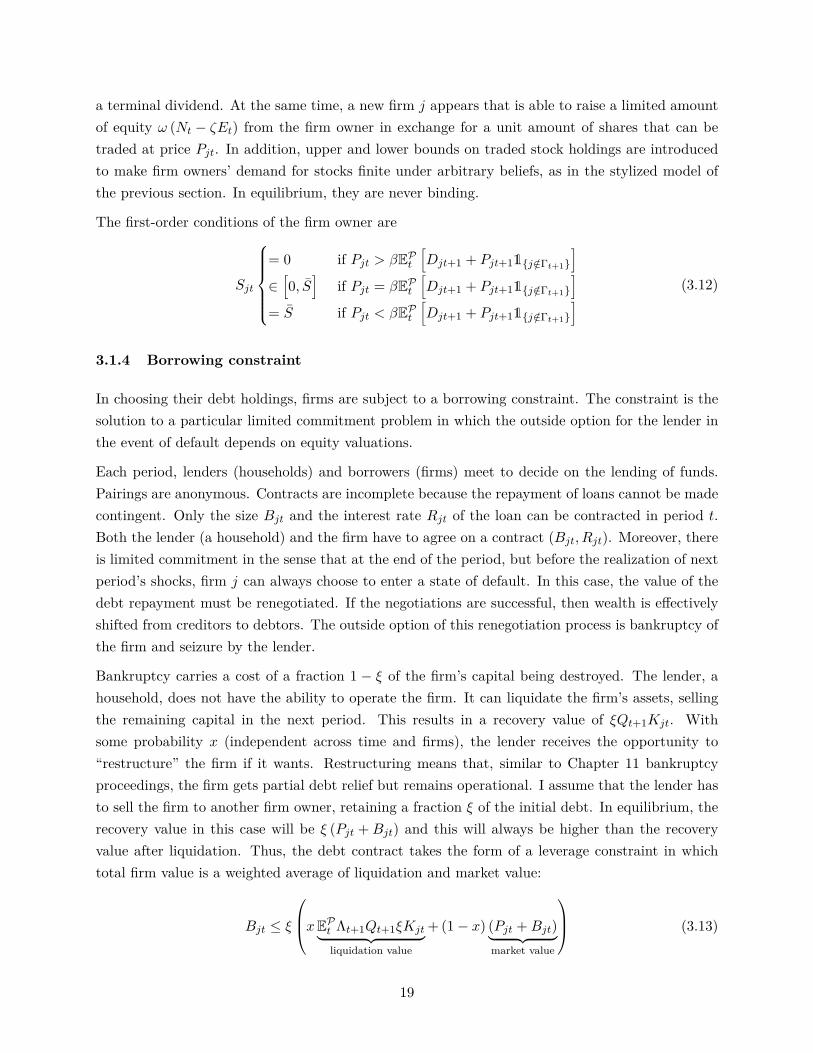
In choosing their debt holdings, firms are subject to a borrowing constraint. The constraint is thesolution to a particular limited commitment problem in which the outside option for the lender inthe event of default depends on equity valuations.

Each period, lenders (households) and borrowers (firms) meet to decide on the lending of funds.Pairings are anonymous. Contracts are incomplete because the repayment of loans cannot be madecontingent. Only the size Bjt and the interest rate Rjt of the loan can be contracted in period t.Both the lender (a household) and the firm have to agree on a contract (Bjt, Rjt). Moreover, thereis limited commitment in the sense that at the end of the period, but before the realization of nextperiod’s shocks, firm j can always choose to enter a state of default. In this case, the value of thedebt repayment must be renegotiated. If the negotiations are successful, then wealth is effectivelyshifted from creditors to debtors. The outside option of this renegotiation process is bankruptcy ofthe firm and seizure by the lender.

Bankruptcy carries a cost of a fraction 1 − ξ of the firm’s capital being destroyed. The lender, ahousehold, does not have the ability to operate the firm. It can liquidate the firm’s assets, sellingthe remaining capital in the next period. This results in a recovery value of ξQt+1Kjt. Withsome probability x (independent across time and firms), the lender receives the opportunity to“restructure” the firm if it wants. Restructuring means that, similar to Chapter 11 bankruptcyproceedings, the firm gets partial debt relief but remains operational. I assume that the lender hasto sell the firm to another firm owner, retaining a fraction ξ of the initial debt. In equilibrium, therecovery value in this case will be ξ (Pjt +Bjt) and this will always be higher than the recoveryvalue after liquidation. Thus, the debt contract takes the form of a leverage constraint in whichtotal firm value is a weighted average of liquidation and market value:

Bjt ≤ ξ

xEPt Λt+1Qt+1ξKjt︸ ︷︷ ︸liquidation value

+ (1− x) (Pjt +Bjt)︸ ︷︷ ︸market value

(3.13)

19

3.1.5 Central bank

The model is cashless, with the central bank setting the nominal interest rate according to aTaylor-type interest rate rule:

it = ρiit−1 + (1− ρi)(β−1 + φππt + εit

), (3.14)

where φπ is the reaction coefficient on inflation, ρi is the degree of interest rate smoothing, and εitis an interest rate shock.

3.1.6 Further model elements and market clearing

Final good producers, indexed by i ∈ [0, 1], combine the homogeneous intermediate good intoa differentiated final good using a one-for-one technology. Their revenue is subsidized by thegovernment at the rate τ .12 Per-period profits of producer i are ΠY

it = (1 + τ) (pit/pt)Yit − qtYit.They are subject to a Calvo price-setting friction: Every period, each final good producer canchange his price only with probability 1 − κ, independent across time and producers. Similarly,labor agencies (indexed by h ∈ [0, 1]) combine the homogeneous labor provided by householdsinto differentiated labor goods which they sell on to intermediate good producers. labor agencies’revenue is subsidized at the rate τw, the per-period profit of agency h is ΠL

ht = (1 + τ) (Wht/pt)Lht−wtLht, and each agency can change its nominal wage Wht only with probability 1 − κw. Thegovernment collects subsidies as lump sum taxes from households and runs a balanced budget eachperiod. The government sets the subsidy rates such that under flexible prices, the markup overmarginal cost is zero in both the labor and output markets.

Capital goods producers produce new capital goods subject to standard investment adjustmentcosts and have profits ΠI

t . Thus, the total amount of lump-sum payments Πt received by thehousehold is the sum of the profits of all final good producers, labor agencies, and capital goodsproducers, minus the sum of all subsidies.

Finally, the exogenous stochastic processes are productivity and the monetary policy shock:

logAt = (1− ρ) log A+ ρ logAt−1 + log εAt (3.15)

εAt ∼ N(0, σ2

A

)(3.16)

εit ∼ N(0, σ2

i

)(3.17)

All market clearing conditions are listed in Appendix A.12This assumption is standard in the New Keynesian literature. It eliminates distortions from monopolistic com-

petition where firms price above marginal cost. The only distortion is then due to sticky prices, which simplifies thesolution by perturbation methods.

20

3.2 Rational expectations equilibrium

I first describe the equilibrium under rational expectations. An equilibrium is a set of stochasticprocesses for prices and allocations, a set of strategies in the limited commitment game, and anexpectation measure P such that the following holds for all states and time periods: Marketsclear; allocations solve the optimization programs of all agents given prices and expectations P;the strategies in the limited commitment game are a subgame-perfect Nash equilibrium for alllender-borrower pairs; and the measure P satisfies rational expectations.

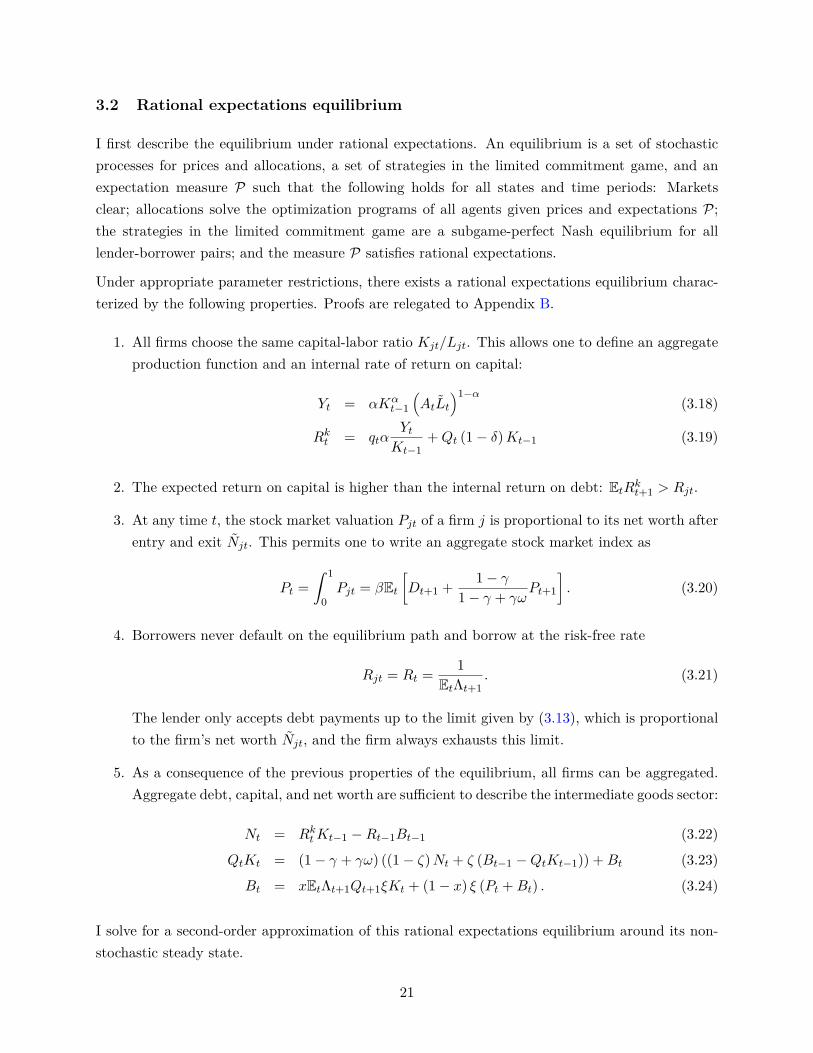
Under appropriate parameter restrictions, there exists a rational expectations equilibrium charac-terized by the following properties. Proofs are relegated to Appendix B.

1. All firms choose the same capital-labor ratio Kjt/Ljt. This allows one to define an aggregateproduction function and an internal rate of return on capital:

Yt = αKαt−1

(AtLt

)1−α(3.18)

Rkt = qtαYtKt−1

+Qt (1− δ)Kt−1 (3.19)

2. The expected return on capital is higher than the internal return on debt: EtRkt+1 > Rjt.

3. At any time t, the stock market valuation Pjt of a firm j is proportional to its net worth afterentry and exit Njt. This permits one to write an aggregate stock market index as

Pt =ˆ 1

0Pjt = βEt

[Dt+1 + 1− γ

1− γ + γωPt+1

]. (3.20)

4. Borrowers never default on the equilibrium path and borrow at the risk-free rate

Rjt = Rt = 1EtΛt+1

. (3.21)

The lender only accepts debt payments up to the limit given by (3.13), which is proportionalto the firm’s net worth Njt, and the firm always exhausts this limit.

5. As a consequence of the previous properties of the equilibrium, all firms can be aggregated.Aggregate debt, capital, and net worth are sufficient to describe the intermediate goods sector:

Nt = RktKt−1 −Rt−1Bt−1 (3.22)

QtKt = (1− γ + γω) ((1− ζ)Nt + ζ (Bt−1 −QtKt−1)) +Bt (3.23)

Bt = xEtΛt+1Qt+1ξKt + (1− x) ξ (Pt +Bt) . (3.24)

I solve for a second-order approximation of this rational expectations equilibrium around its non-stochastic steady state.

21

3.3 Learning equilibrium

I introduce learning about stock market valuations, as in the simple model of Section 2. There isnow a continuum of firms to be priced in the market, and I retain the belief that the stock price ofan individual firm is proportional to firm net worth, as is the case under rational expectations. Assuch, under P,

Pjt = Njt

NtPt. (3.25)

But while investors know how to price individual stocks by observing the valuation of the market,they are uncertain about the evolution of the market itself. As in the simple model of the previoussection, I impose the same beliefs about aggregate stock prices as in the last section along withthe other assumptions (equations (2.20)–(2.23)), including expectations on other variables that areconditionally consistent with outcomes on the equilibrium path: For any variable xt, any date t,and any sequence P0, . . . , Pt that is on the equilibrium path, agents’ beliefs coincide with the beststatistical prediction of xt conditional on the realization of stock prices.

In practice, I solve the model using a two-stage procedure. The first stage is to solve for the policyfunctions and beliefs under P. The Kalman filtering equations that describe beliefs about stockprices are as follows:

logPt = logPt−1 + µt−1 −σ2ν + σ2

η

2 + zt (3.26)

µt = µt−1 −σ2ν

2 + gzt, (3.27)

where µt is the mean belief about the trend in stock price growth, and zt is the forecast error.Under the subjective beliefs P, it is normally distributed white noise. I impose that beliefs aboutany other endogenous variable are consistent with model outcomes conditional on the evolution ofstock prices, and so beliefs and policy functions can be calculated much in the same way as underrational expectations, taking zt as an exogenous shock process. The market clearing condition forstocks does not enter this first stage of the problem. Adding it would effectively require that beliefsabout stock prices, too, be consistent with equilibrium outcomes—and the solution would collapseto the rational expectations equilibrium. Now, if xt is the set of model variables and ut the set ofexogenous shocks, solving this first stage leads to a subjective policy function xt = h (xt−1, ut, zt).

The second stage of the model consists in finding the value for zt which leads to market clearingin the stock market and thereby establishes equilibrium. This results in a mapping from the statevariables and exogenous shocks to the perceived forecast error r : (xt−1, ut) 7→ zt. Clearly, thisfunction generally does not make zt an iid disturbance in equilibrium. This is why agents makesystematic forecast errors. The complete solution of the model is given by xt = g (xt−1, ut) =h (xt−1, ut, r (xt−1, ut)). A complete description of a second-order perturbation of this solution iscontained in Appendix C.

22

3.4 Choice of parameters

I partition the set of parameters into two groups. The first set of parameters is calibrated tofirst-order moments, and the second set is estimated by simulated method of moments (SMM) onsecond-order moments of US quarterly data.

3.4.1 Calibration

The capital share in production is set to α = 0.33, implying a labor share in output of two thirds.The depreciation rate δ = 0.025 corresponds to 10 percent annual depreciation. The persistence ofthe temporary component of productivity is set to 0.95.

The discount factor is set such that the steady-state interest rate matches the average annual realreturn on Treasury bills of 2.5 percent, implying a discount factor β = 0.9938. The elasticity ofsubstitution between varieties of the final consumption good, as well as that among varieties oflabor used in production, is set to σ = σw = 4. The Frisch elasticity of labor supply is set to 3,implying φ = 0.33.

The strength of monetary policy reaction to inflation is set to φπ = 1.5, and the degree of nominalrate smoothing is set to ρi = 0.85.

Four parameters describe the structure of financial constraints: x, the probability of restructuringafter default; ξ, the tightness of the borrowing constraint; ω, the equity received by new firmsrelative to average equity; and γ, the rate of firm exit and entry. I calibrate the restructuringrate to x = 0.093. This is the fraction of US business bankruptcy filings in 2006 that filed forChapter 11 instead of Chapter 7, and that subsequently emerged from bankruptcy with an approvedrestructuring plan (a sensitivity check is included in Section 5.2).13 The remaining three parametersare chosen such that the non-stochastic steady state of the model jointly matches the US averageinvestment share in output of 20 percent, average debt-to-equity ratio of 1:1 (as recorded in the Fedflow of funds), and average quarterly P/D ratio of 139 (taken from the S&P500). The parametervalues thus are γ = 0.0165, ξ = 0.4152, and ω = 0.018.

3.4.2 Estimation

The remaining parameters are the standard deviations of the technology and monetary shocks(σA, σi), the degree of nominal price and wage rigidities (κ, κw), the size of investment adjustmentcosts (ψ), the fraction of dividends paid out as earnings by continuing firms (ζ), and the learninggain (g). I estimate these six parameters to minimize the distance to a set of eight moments

132006 is the only year for which this number can be constructed from publicly available data. Data on bankruptciesby chapter are available at http://www.uscourts.gov/Statistics/BankruptcyStatistics.aspx. Data on Chapter11 outcomes are analyzed in various samples by Flynn and Crewson (2009), Warren and Westbrook (2009), Lawton(2012), and Altman (2014).

23

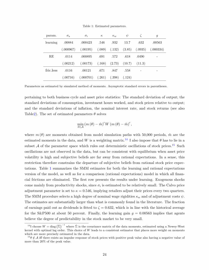
Table 1: Estimated parameters.

param. σa σi κ κw ψ ζ g

learning .00884 .000423 .546 .932 13.7 .632 .00563

(.000967) (.00195) (.089) (.132) (3.85) (.0935) (.000334)

RE .0114 .000895 .691 .572 .618 .0490 -

(.00212) (.00173) (.168) (2.73) (10.7) (11.3)

fric.less .0116 .00121 .671 .847 .558 - -

(.00716) (.000701) (.261) (.398) (.124)

Parameters as estimated by simulated method of moments. Asymptotic standard errors in parentheses.

pertaining to both business cycle and asset price statistics: The standard deviation of output; thestandard deviations of consumption, investment hours worked, and stock prices relative to output;and the standard deviations of inflation, the nominal interest rate, and stock returns (see alsoTable2). The set of estimated parameters θ solves

minϑ∈A

(m (θ)− m)′W (m (θ)− m)′ ,

where m (θ) are moments obtained from model simulation paths with 50,000 periods, m are theestimated moments in the data, and W is a weighting matrix.14 I also impose that θ has to lie in asubset A of the parameter space which rules out deterministic oscillations of stock prices.15 Suchoscillations are not observed in the data, but can be consistent with equilibrium when asset pricevolatility is high and subjective beliefs are far away from rational expectations. In a sense, thisrestriction therefore constrains the departure of subjective beliefs from rational stock price expec-tations. Table 1 summarizes the SMM estimates for both the learning and rational expectationsversion of the model, as well as for a comparison (rational expectations) model in which all finan-cial frictions are eliminated. The first row presents the results under learning. Exogenous shockscome mainly from productivity shocks, since σi is estimated to be relatively small. The Calvo priceadjustment parameter is set to κ = 0.546, implying retailers adjust their prices every two quarters.The SMM procedure selects a high degree of nominal wage rigidities κw and of adjustment costs ψ.The estimates are substantially larger than what is commonly found in the literature. The fractionof earnings paid out as dividends is fitted to ζ = 0.632, which is in line with the historical averagefor the S&P500 at about 50 percent. Finally, the learning gain g = 0.00563 implies that agentsbelieve the degree of predictability in the stock market to be very small.

14I choose W = diag(Σ)−1 where Σ is the covariance matrix of the data moments, estimated using a Newey-West

kernel with optimal lag order. This choice of W leads to a consistent estimator that places more weight on momentswhich are more precisely estimated in the data.

15θ /∈ A iff there exists an impulse response of stock prices with positive peak value also having a negative value ofmore than 20% of the peak value.

24

The second row contains the parameters estimated under rational expectations. The fit to theasset price moments included in the estimation is worse and the asymptotic standard errors arelarge, implying that the distance of the moments to the data at the point estimate is relatively flat.Nevertheless, at this point estimate, the size of the shocks σa and σi is substantially larger underlearning. This implies that learning about stock prices leads to substantial amplification of shocks:The increased endogenous volatility of asset prices greatly magnifies the financial accelerator effect,just as in the simple model of Section 2. The degree of wage rigidities and investment adjustmentcosts required to fit the data is smaller than under learning.

The third row contains parameter estimates under the model without financial frictions (and ratio-nal expectations). Since the financial structure is eliminated from that model, the dividend payoutratio ζ is not present. The size of the shocks is larger than under the rational expectations modelwith the financial accelerator present. This points to moderate amplification effects of financialfrictions under rational expectations.

4 Results

I now present the quantitative results of this paper. First, I review standard business cycle statistics.Learning and asset price volatility account for more than a third of the volatility of output, pointingto the strength of the endogenous amplification mechanism. In contrast, the financial acceleratormechanism under rational expectations is relatively weak. I then look at asset pricing moments andfind that the model with learning closely matches not only the volatility of stock prices (which istargeted by the estimation), but also the predictability of stock returns as well as negative skewnessand excess kurtosis. Under rational expectations, all these statistics are close to zero even thoughthe estimation tries to target asset price volatility. Next, I present impulse response functionsto both supply and demand shocks, confirming the strong amplification mechanism in all mainmacroeconomic aggregates. The main element is the endogenous volatility of asset prices inducedby learning, leading to very procyclical credit constraints. But I also show that this is not thewhole story: The fact that agents are too optimistic about future asset prices during expansionsand vice-versa affects aggregate demand, adding additional amplification that is unique to a modelwith learning. Finally, I compare forecast errors made by agents in the model with those observedin actual survey data. The patterns of predictability are remarkably similar, lending credibility tothe chosen expectation formation process.

4.1 Business cycle and asset price moments

To get a better understanding of the quantitative properties of the model, I review key momentsin the data and across model specifications. Table 2 starts with business cycle statistics. Thedata moments are in Column (1). Moments for the estimated learning model are in Column

25

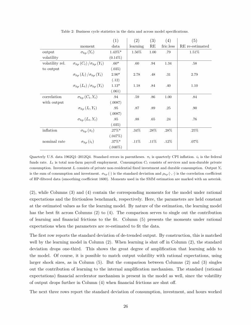
Table 2: Business cycle statistics in the data and across model specifications.

(1) (2) (3) (4) (5)moment data learning RE fric.less RE re-estimated

outputvolatility

σhp (Yt) 1.43%*(0.14%)

1.56% 1.00 .79 1.51%

volatility rel.to output

σhp (Ct) /σhp (Yt) .60*(.035)

.60 .94 1.34 .58

σhp (It) /σhp (Yt) 2.90*(.12)

2.78 .48 .31 2.79

σhp (Lt) /σhp (Yt) 1.13*(.061)

1.18 .84 .40 1.10

correlationwith output

σhp (Ct, Yt) .94(.0087)

.59 .86 1.00 .84

σhp (It, Yt) .95(.0087)

.87 .89 .25 .90

σhp (Lt, Yt) .85(.035)

.88 .65 .24 .76

inflation σhp (πt) .27%*(.047%)

.34% .28% .28% .25%

nominal rate σhp (it) .37%*(.046%)

.11% .11% .12% .07%

Quarterly U.S. data 1962Q1–2012Q4. Standard errors in parentheses. πt is quarterly CPI inflation. it is the federalfunds rate. Lt is total non-farm payroll employment. Consumption Ct consists of services and non-durable privateconsumption. Investment It consists of private non-residential fixed investment and durable consumption. Output Ytis the sum of consumption and investment. σhp (·) is the standard deviation and ρhp (·, ·) is the correlation coefficientof HP-filtered data (smoothing coefficient 1600). Moments used in the SMM estimation are marked with an asterisk.

(2), while Columns (3) and (4) contain the corresponding moments for the model under rationalexpectations and the frictionless benchmark, respectively. Here, the parameters are held constantat the estimated values as for the learning model. By nature of the estimation, the learning modelhas the best fit across Columns (2) to (4). The comparison serves to single out the contributionof learning and financial frictions to the fit. Column (5) presents the moments under rationalexpectations when the parameters are re-estimated to fit the data.

The first row reports the standard deviation of de-trended output. By construction, this is matchedwell by the learning model in Column (2). When learning is shut off in Column (2), the standarddeviation drops one-third. This shows the great degree of amplification that learning adds tothe model. Of course, it is possible to match output volatility with rational expectations, usinglarger shock sizes, as in Column (5). But the comparison between Columns (2) and (3) singlesout the contribution of learning to the internal amplification mechanism. The standard (rationalexpectations) financial accelerator mechanism is present in the model as well, since the volatilityof output drops further in Column (4) when financial frictions are shut off.

The next three rows report the standard deviation of consumption, investment, and hours worked

26

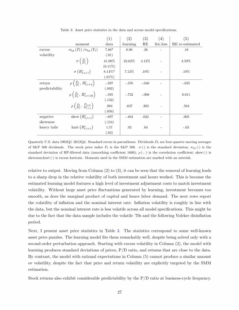
Table 3: Asset price statistics in the data and across model specifications.

(1) (2) (3) (4) (5)moment data learning RE fric.less RE re-estimated

excessvolatility

σhp (Pt) /σhp (Yt) 7.86*(.61)

8.96 .26 - .16

σ(PtDt

)41.08%(6.11%)

22.62% 4.12% - 3.59%

σ(Ret,t+1

)8.14%*(.61%)

7.12% .19% - .19%

returnpredictability

ρ(PtDt, Ret,t+4

)-.297(.092)

-.376 -.040 - -.035

ρ(PtDt, Ret,t+20

)-.585(.132)

-.732 -.006 - 0.011

ρ(PtDt, Pt+4Dt+4

).904(.056)

.637 .303 - .564

negativeskewness

skew(Ret,t+1

)-.897(.154)

-.404 .022 - .005

heavy tails kurt(Ret,t+1

)1.57(.62)

.92 .04 - -.03

Quarterly U.S. data 1962Q1–2012Q4. Standard errors in parentheses. Dividends Dt are four-quarter moving averagesof S&P 500 dividends. The stock price index Pt is the S&P 500. σ (·) is the standard deviation; σhp (·) is thestandard deviation of HP-filtered data (smoothing coefficient 1600); ρ (·, ·) is the correlation coefficient; skew (·) isskewness;kurt (·) is excess kurtosis. Moments used in the SMM estimation are marked with an asterisk.

relative to output. Moving from Column (2) to (3), it can be seen that the removal of learning leadsto a sharp drop in the relative volatility of both investment and hours worked. This is because theestimated learning model features a high level of investment adjustment costs to match investmentvolatility. Without large asset price fluctuations generated by learning, investment becomes toosmooth, as does the marginal product of capital and hence labor demand. The next rows reportthe volatility of inflation and the nominal interest rate. Inflation volatility is roughly in line withthe data, but the nominal interest rate is less volatile across all model specifications. This might bedue to the fact that the data sample includes the volatile ’70s and the following Volcker disinflationperiod.

Next, I present asset price statistics in Table 3. The statistics correspond to some well-knownasset price puzzles. The learning model fits them remarkably well, despite being solved only with asecond-order perturbation approach. Starting with excess volatility in Column (2), the model withlearning produces standard deviations of prices, P/D ratio, and returns that are close to the data.By contrast, the model with rational expectations in Column (5) cannot produce a similar amountov volatility, despite the fact that price and return volatility are explicitly targeted by the SMMestimation.

Stock returns also exhibit considerable predictability by the P/D ratio at business-cycle frequency.

27

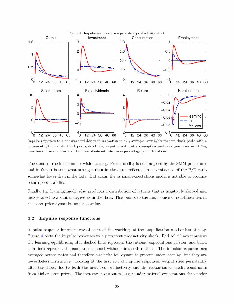
Figure 4: Impulse responses to a persistent productivity shock.

0 12 24 36 48 600

0.5

1

1.5Output

0 12 24 36 48 60−1

0

1

2

3Investment

0 12 24 36 48 600

0.2

0.4

0.6

0.8Consumption

0 12 24 36 48 60−1

−0.5

0

0.5

1Employment

0 12 24 36 48 60−5

0

5

10Stock prices

0 12 24 36 48 60−4

−2

0

2

4Exp. dividends

0 12 24 36 48 60−2

0

2

4Return

0 12 24 36 48 60−0.1

−0.08

−0.06

−0.04

−0.02

0Nominal rate

learning

RE

fric.less

Impulse responses to a one-standard deviation innovation in εAt, averaged over 5,000 random shock paths with aburn-in of 1,000 periods. Stock prices, dividends, output, investment, consumption, and employment are in 100*logdeviations. Stock returns and the nominal interest rate are in percentage point deviations.

The same is true in the model with learning. Predictability is not targeted by the SMM procedure,and in fact it is somewhat stronger than in the data, reflected in a persistence of the P/D ratiosomewhat lower than in the data. But again, the rational expectations model is not able to producereturn predictability.

Finally, the learning model also produces a distribution of returns that is negatively skewed andheavy-tailed to a similar degree as in the data. This points to the importance of non-linearities inthe asset price dynamics under learning.

4.2 Impulse response functions

Impulse response functions reveal some of the workings of the amplification mechanism at play.Figure 4 plots the impulse responses to a persistent productivity shock. Red solid lines representthe learning equilibrium, blue dashed lines represent the rational expectations version, and blackthin lines represent the comparison model without financial frictions. The impulse responses areaveraged across states and therefore mask the tail dynamics present under learning, but they arenevertheless instructive. Looking at the first row of impulse responses, output rises persistentlyafter the shock due to both the increased productivity and the relaxation of credit constraintsfrom higher asset prices. The increase in output is larger under rational expectations than under

28

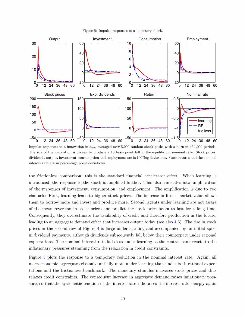
Figure 5: Impulse responses to a monetary shock.

0 12 24 36 48 600

10

20

30Output

0 12 24 36 48 60−20

0

20

40

60Investment

0 12 24 36 48 600

2

4

6

8

10Consumption

0 12 24 36 48 60−20

0

20

40

60Employment

0 12 24 36 48 60−50

0

50

100

150

200Stock prices

0 12 24 36 48 60−50

0

50

100

150Exp. dividends

0 12 24 36 48 60−50

0

50

100

150Return

0 12 24 36 48 60−1.5

−1

−0.5

0

0.5Nominal rate

learning

RE

fric.less

Impulse responses to a innovation in εmt, averaged over 5,000 random shock paths with a burn-in of 1,000 periods.The size of the innovation is chosen to produce a 10 basis point fall in the equilibrium nominal rate. Stock prices,dividends, output, investment, consumption and employment are in 100*log deviations. Stock returns and the nominalinterest rate are in percentage point deviations.

the frictionless comparison; this is the standard financial accelerator effect. When learning isintroduced, the response to the shock is amplified further. This also translates into amplificationof the responses of investment, consumption, and employment. The amplification is due to twochannels: First, learning leads to higher stock prices. The increase in firms’ market value allowsthem to borrow more and invest and produce more. Second, agents under learning are not awareof the mean reversion in stock prices and predict the stock price boom to last for a long time.Consequently, they overestimate the availability of credit and therefore production in the future,leading to an aggregate demand effect that increases output today (see also 4.3). The rise in stockprices in the second row of Figure 4 is large under learning and accompanied by an initial spikein dividend payments, although dividends subsequently fall below their counterpart under rationalexpectations. The nominal interest rate falls less under learning as the central bank reacts to theinflationary pressures stemming from the relaxation in credit constraints.

Figure 5 plots the response to a temporary reduction in the nominal interest rate. Again, allmacroeconomic aggregates rise substantially more under learning than under both rational expec-tations and the frictionless benchmark. The monetary stimulus increases stock prices and thusrelaxes credit constraints. The consequent increase in aggregate demand raises inflationary pres-sure, so that the systematic reaction of the interest rate rule raises the interest rate sharply again

29

after the shock.

4.3 Does learning matter?

The discussion so far has mainly focused on how large swings in asset prices lead to large swingsin real activity through their effect on credit constraints. But is learning necessary for this storyat all? Maybe all that matters for amplification is that asset price volatility has to be increased,by some mechanism or other. In this section, I show that learning has an effect on amplificationover and above its effect on asset prices.

I replace the stock market value Pt in the borrowing constraint (3.24) with an exogenous processVt that has the same law of motion as the stock price under learning. More precisely, I fit anARMA(10,5) process for Vt such that its impulse responses are as close as possible to those ofPt under learning (the exogenous shock in the ARMA process are the productivity and monetaryshocks). I then solve this model, but with rational expectations. If learning only matters because itaffects stock price dynamics, then this hypothetical model should have exactly identical dynamicsto the model under learning.16

Figure 6 shows that this is not the case. The ARMA process fits stock prices well: The impulseresponse of Pt under learning and Vt in the counterfactual experiment are indistinguishable. Butafter a positive productivity shock, output, investment, and consumption rise more under learning,even though the counterfactual model has the same stock price dynamics by construction. Thereason is that expectations of future asset prices matter beyond their direct impact on currentprices. Under learning, agents do not fully internalize mean reversion in stock prices and thereforepredict that credit constraints are loose for longer than they turn out to be. This leads to awealth effect on households that increases their consumption, raising aggregate demand, and itleads to higher future expected prices of capital goods EtQt+1, which enters the liquidation value offirms and hence relaxes borrowing constraints, even if stock prices are the same as under rationalexpectations. These effects are powerful enough to create significant endogenous amplificationthrough the departure of subjective beliefs from rational expectations.

4.4 Relation to survey evidence on expectations

The rational expectations hypothesis asserts that “outcomes do not differ systematically [...] fromwhat people expect them to be” (Sargent, 2008). Put differently, a forecast error should not besystematically predictable by information available at the time of the forecast. The absence ofpredictability is almost always rejected in the data.

Similarly, agents in the model under learning also make systematic, predictable forecast errors.This holds not only for stock prices but also other endogenous model variables, despite the fact

16For this exercise I only compute a first-order approximation to the model equations.

30

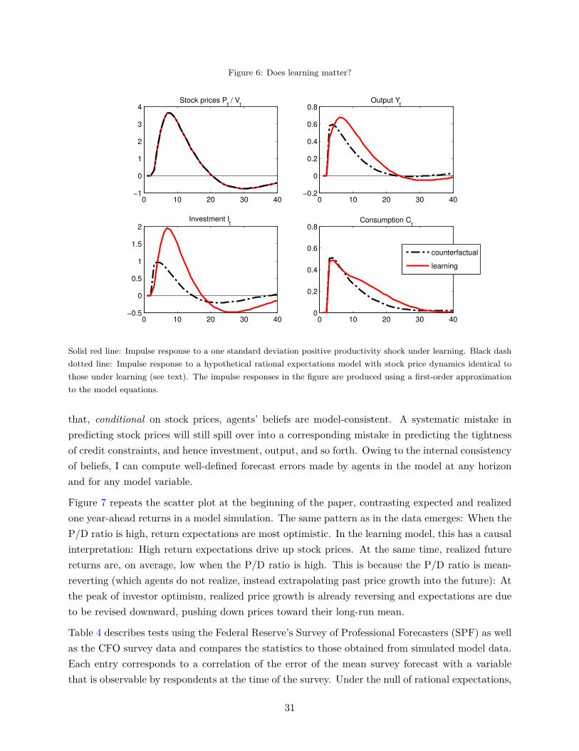
Figure 6: Does learning matter?

0 10 20 30 40−1

0

1

2

3

4Stock prices P

t / V

t

0 10 20 30 40−0.2

0

0.2

0.4

0.6

0.8Output Y

t

0 10 20 30 40−0.5

0

0.5

1

1.5

2Investment I

t

0 10 20 30 400

0.2

0.4

0.6

0.8Consumption C

t

counterfactual

learning

Solid red line: Impulse response to a one standard deviation positive productivity shock under learning. Black dashdotted line: Impulse response to a hypothetical rational expectations model with stock price dynamics identical tothose under learning (see text). The impulse responses in the figure are produced using a first-order approximationto the model equations.

that, conditional on stock prices, agents’ beliefs are model-consistent. A systematic mistake inpredicting stock prices will still spill over into a corresponding mistake in predicting the tightnessof credit constraints, and hence investment, output, and so forth. Owing to the internal consistencyof beliefs, I can compute well-defined forecast errors made by agents in the model at any horizonand for any model variable.

Figure 7 repeats the scatter plot at the beginning of the paper, contrasting expected and realizedone year-ahead returns in a model simulation. The same pattern as in the data emerges: When theP/D ratio is high, return expectations are most optimistic. In the learning model, this has a causalinterpretation: High return expectations drive up stock prices. At the same time, realized futurereturns are, on average, low when the P/D ratio is high. This is because the P/D ratio is mean-reverting (which agents do not realize, instead extrapolating past price growth into the future): Atthe peak of investor optimism, realized price growth is already reversing and expectations are dueto be revised downward, pushing down prices toward their long-run mean.

Table 4 describes tests using the Federal Reserve’s Survey of Professional Forecasters (SPF) as wellas the CFO survey data and compares the statistics to those obtained from simulated model data.Each entry corresponds to a correlation of the error of the mean survey forecast with a variablethat is observable by respondents at the time of the survey. Under the null of rational expectations,

31

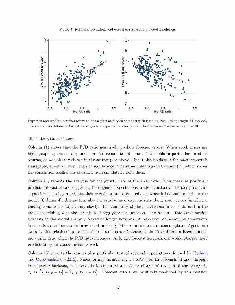
Figure 7: Return expectations and expected returns in a model simulation.

2.2

2.4

2.6

2.8

33.

21-

year

ret

urn

fore

cast

3.4 3.6 3.8 4 4.2log P/D ratio

-60

-40

-20

020

4060

1-ye

ar r

ealis

ed r

etur

n

3.4 3.6 3.8 4 4.2log P/D ratio

Expected and realized nominal returns along a simulated path of model with learning. Simulation length 200 periods.Theoretical correlation coefficient for subjective expected returns ρ = .47, for future realized returns ρ = −.38.

all entries should be zero.

Column (1) shows that the P/D ratio negatively predicts forecast errors. When stock prices arehigh, people systematically under-predict economic outcomes. This holds in particular for stockreturns, as was already shown in the scatter plot above. But it also holds true for macroeconomicaggregates, albeit at lower levels of significance. The same holds true in Column (2), which showsthe correlation coefficients obtained from simulated model data.

Column (3) repeats the exercise for the growth rate of the P/D ratio. This measure positivelypredicts forecast errors, suggesting that agents’ expectations are too cautious and under-predict anexpansion in its beginning but then overshoot and over-predict it when it is about to end. In themodel (Column 4), this pattern also emerges because expectations about asset prices (and hencelending conditions) adjust only slowly. The similarity of the correlations in the data and in themodel is striking, with the exception of aggregate consumption. The reason is that consumptionforecasts in the model are only biased at longer horizons: A relaxation of borrowing constraintsfirst leads to an increase in investment and only later to an increase in consumption. Agents areaware of this relationship, so that their three-quarter forecasts, as in Table 4 do not become muchmore optimistic when the P/D ratio increases. At longer forecast horizons, one would observe morepredictability for consumption as well.

Column (5) reports the results of a particular test of rational expectations devised by Coibionand Gorodnichenko (2015). Since for any variable xt, the SPF asks for forecasts at one- throughfour-quarter horizons, it is possible to construct a measure of agents’ revision of the change inxt as Et [xt+3 − xt] − Et−1 [xt+3 − xt]. Forecast errors are positively predicted by this revision

32

Table 4: Forecast errors under learning and in the data.

(1) (2) (3) (4) (5) (6)logPDt ∆ logPDt forecast revision

forecast variable data model data model data modelRstockt,t+4 -.44 -.38 .06 .30 - -.30

(-3.42) (.41)Yt,t+3 -.21 -.16 .22 .16 .29 .28

(-1.78) (2.42) (3.83)It,t+3 -.20 -.37 .25 .27 .31 .35

(-1.74) (2.88) (3.79)Ct,t+3 -.19 -.04 .21 .01 .23 .02

(-1.85) (2.37) (2.67)ut,t+3 .05 .20 -.27 -.20 .43 .32

(.12) (-3.07) (6.07)

Correlation coefficients for mean forecast errors on one year-ahead nominal stock returns (Graham-Harvey survey)and three quarters-ahead real output growth, investment growth, consumption growth and the unemployment rate(SPF). t-statistics in parentheses. Regressors: Column (1) is the S&P 500 P/D ratio and Column (2) is its firstdifference. Column (3) is the forecast revision, as in Coibion and Gorodnichenko (2015). Data from Graham-Harveycovers 2000Q3–2012Q4. Data for the SPF covers 1981Q1–2012Q4. For the model, correlations are computed usinga simulation of length 50,000, where subjective forecasts are computed using a second-order approximation to thesubjective belief system on a path in which no more future shocks occur, starting at the current state in each period.Unemployment in the model is taken to be ut = 1− Lt.

measure. Coibion and Gorodnichenko take this as evidence for sticky information models in whichinformation sets are gradually updated over time. But it is also consistent with the learning model:The correlation coefficients in Column (6) are very similar to those in the data.17

The spill-over of expectational errors is illustrated graphically in Figure 8. The solid red line is astandard impulse response function to a technology shock in the learning model. The green dashedline of Figure 4 depicts agents’ average subjective forecast at the peak of the stock market boomfollowing the shock. Agents do not foresee the decline in the stock market and instead extrapolatehigh stock price growth into the future. Because stock market valuations matter for access to credit,agents also forecast loose borrowing conditions and are too optimistic about output, investment,and (to a lesser extent) consumption, as in the data. The green dashed line (expectations) is abovethe red solid line (realization) when the P/D ratio is high: It negatively predicts forecast errors.The blue dotted line is the forecast made at a time in which the P/D ratio is rising. In this situation,agents under-predict the size of the coming boom in the stock market and real activity. Therefore,the growth rate of the P/D ratio positively predicts forecast errors.

17The model predicts a negative correlation of forecast errors on stock returns with their forecast revisions. The CFOsurvey does not allow for the construction of the corresponding statistic in the data, but it is an interesting implicationsince a negative correlation cannot be produced by rigid information models as in Coibion and Gorodnichenko.

33

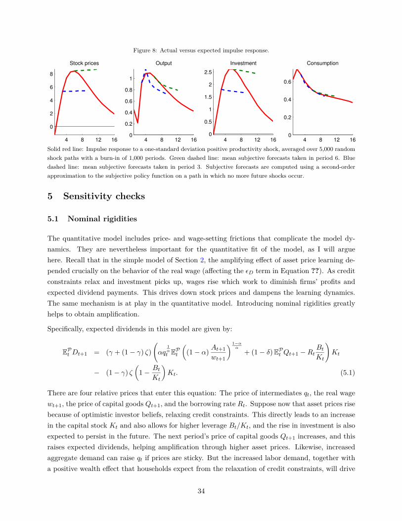
Figure 8: Actual versus expected impulse response.

4 8 12 16

0

2

4

6

8

Stock prices

4 8 12 160

0.2

0.4

0.6

0.8

1

Output

4 8 12 160

0.5

1

1.5

2

2.5

Investment

4 8 12 160

0.2

0.4

0.6

Consumption

Solid red line: Impulse response to a one-standard deviation positive productivity shock, averaged over 5,000 randomshock paths with a burn-in of 1,000 periods. Green dashed line: mean subjective forecasts taken in period 6. Bluedashed line: mean subjective forecasts taken in period 3. Subjective forecasts are computed using a second-orderapproximation to the subjective policy function on a path in which no more future shocks occur.

5 Sensitivity checks

5.1 Nominal rigidities

The quantitative model includes price- and wage-setting frictions that complicate the model dy-namics. They are nevertheless important for the quantitative fit of the model, as I will arguehere. Recall that in the simple model of Section 2, the amplifying effect of asset price learning de-pended crucially on the behavior of the real wage (affecting the εD term in Equation ??). As creditconstraints relax and investment picks up, wages rise which work to diminish firms’ profits andexpected dividend payments. This drives down stock prices and dampens the learning dynamics.The same mechanism is at play in the quantitative model. Introducing nominal rigidities greatlyhelps to obtain amplification.

Specifically, expected dividends in this model are given by:

EPt Dt+1 = (γ + (1− γ) ζ)(αq

1αt EPt

((1− α) At+1

wt+1

) 1−αα

+ (1− δ)EPt Qt+1 −RtBtKt

)Kt

− (1− γ) ζ(

1− BtKt

)Kt. (5.1)

There are four relative prices that enter this equation: The price of intermediates qt, the real wagewt+1, the price of capital goods Qt+1, and the borrowing rate Rt. Suppose now that asset prices risebecause of optimistic investor beliefs, relaxing credit constraints. This directly leads to an increasein the capital stock Kt and also allows for higher leverage Bt/Kt, and the rise in investment is alsoexpected to persist in the future. The next period’s price of capital goods Qt+1 increases, and thisraises expected dividends, helping amplification through higher asset prices. Likewise, increasedaggregate demand can raise qt if prices are sticky. But the increased labor demand, together witha positive wealth effect that households expect from the relaxation of credit constraints, will drive

34

up the real wage wt. This will tend to reduce Dt+1 and dampen the expansion. Also, to the extentthat higher investment comes at the expense of lower consumption in the economy, real borrowingrates Rt will rise, also dampening the expansion. This latter effect is stronger the more leveragethere is in the economy.

Nominal rigidities have effects on real wages, the price of intermediates, and real rates. Wagerigidities will counteract the dampening effects of real wage responses to shocks, allowing for greaterdividend, and therefore asset price, volatility. They also lead to amplification in the response ofemployment to movements in financial market sentiment. Price rigidities, together with a relativelyloose monetary policy rule, imply that the prices of intermediates qt are pro-cyclical, and lead tosmaller real interest rates movements in response to changes in investor sentiment, also helpingamplification. The mirror image of this result, through the consumption Euler equation, is thatconsumption is not pushed down as much by increases in investment, so its response, too, isamplified. In sum, nominal price and wage rigidities allow for comovement of all macroeconomicaggregates in response to changes in subjective beliefs. This co-movement property obtains moregenerally and has been documented in the context of news shocks (Kobayashi and Nutahara, 2010)and financial shocks Ajello (2016).

To illustrate this point, I re-compute impulse responses of the model with learning, but withoutnominal rigidities—i.e., setting κ = κw = 0. I also reduce the size of investment adjustmentcosts to ψ = 0.125. With the high degree of adjustment costs in the baseline version, the modelwould include an explosive two-period oscillation and reducing ψ ensures stability. The low costsof adjusting investment also gives the real version a better chance at delivering strong impulseresponses. Even then, the nominal version delivers far greater amplification. Figure 9 plots impulseresponses to a positive productivity shock for the baseline and the real versions of the model.Owing to lower adjustment costs, the initial response of investment is expectedly stronger in thereal version. However, the real wage wt rises by much more, and also the price of intermediatesqt is fixed, so dividends do not rise as much after the shock. This considerably dampens thelearning dynamics and mutes the response of stock prices. By consequence, the response of output,investment, consumption and hours worked (not shown) is overall weaker than in the baselineversion of the model.

5.2 Borrowing constraint parameters

I will now briefly discuss the sensitivity of the results to the two main parameters affecting theborrowing constraint (3.24): The probability x that a firm can be sold as a going concern afterfiling for bankruptcy, governing the dependency of the constraint on stock prices; and the fractionof assets ξ preserved in bankruptcy, governing the overall tightness of the constraint. Figure 10plots the standard deviation of output and stock prices as a function of these two parameters,respectively.

35

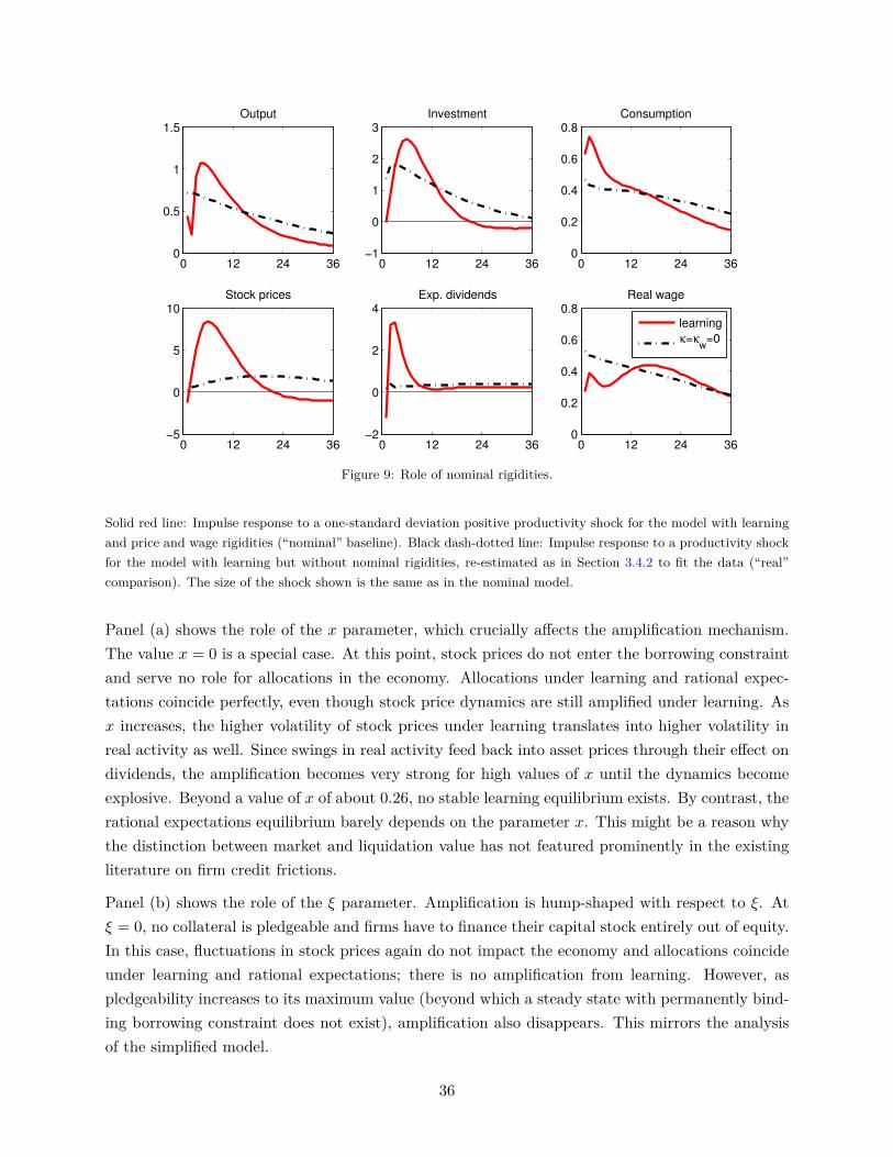
0 12 24 360

0.5

1

1.5Output

0 12 24 36−1

0

1

2

3Investment

0 12 24 360

0.2

0.4

0.6

0.8Consumption

0 12 24 36−5

0

5

10Stock prices

0 12 24 36−2

0

2

4Exp. dividends

0 12 24 360

0.2

0.4

0.6

0.8Real wage

learning

κ=κw

=0

Figure 9: Role of nominal rigidities.

Solid red line: Impulse response to a one-standard deviation positive productivity shock for the model with learningand price and wage rigidities (“nominal” baseline). Black dash-dotted line: Impulse response to a productivity shockfor the model with learning but without nominal rigidities, re-estimated as in Section 3.4.2 to fit the data (“real”comparison). The size of the shock shown is the same as in the nominal model.

Panel (a) shows the role of the x parameter, which crucially affects the amplification mechanism.The value x = 0 is a special case. At this point, stock prices do not enter the borrowing constraintand serve no role for allocations in the economy. Allocations under learning and rational expec-tations coincide perfectly, even though stock price dynamics are still amplified under learning. Asx increases, the higher volatility of stock prices under learning translates into higher volatility inreal activity as well. Since swings in real activity feed back into asset prices through their effect ondividends, the amplification becomes very strong for high values of x until the dynamics becomeexplosive. Beyond a value of x of about 0.26, no stable learning equilibrium exists. By contrast, therational expectations equilibrium barely depends on the parameter x. This might be a reason whythe distinction between market and liquidation value has not featured prominently in the existingliterature on firm credit frictions.

Panel (b) shows the role of the ξ parameter. Amplification is hump-shaped with respect to ξ. Atξ = 0, no collateral is pledgeable and firms have to finance their capital stock entirely out of equity.In this case, fluctuations in stock prices again do not impact the economy and allocations coincideunder learning and rational expectations; there is no amplification from learning. However, aspledgeability increases to its maximum value (beyond which a steady state with permanently bind-ing borrowing constraint does not exist), amplification also disappears. This mirrors the analysisof the simplified model.

36

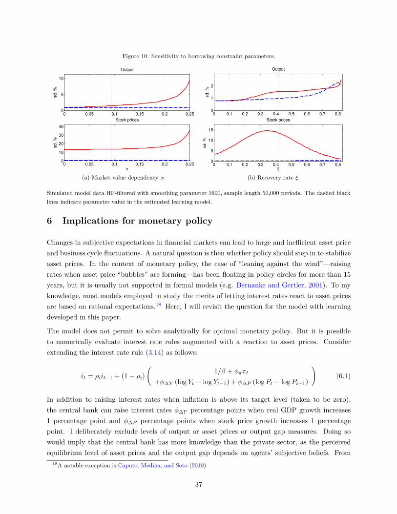
Figure 10: Sensitivity to borrowing constraint parameters.

0 0.05 0.1 0.15 0.2 0.250

5

10

sd

. %

Output

0 0.05 0.1 0.15 0.2 0.250

10

20

30

40

sd

. %

Stock prices

x

(a) Market value dependency x.

0 0.1 0.2 0.3 0.4 0.5 0.6 0.7 0.80

1

2

sd

. %

Output

0 0.1 0.2 0.3 0.4 0.5 0.6 0.7 0.80

5

10

15

sd

. %

Stock prices

ξ

(b) Recovery rate ξ.

Simulated model data HP-filtered with smoothing parameter 1600, sample length 50,000 periods. The dashed blacklines indicate parameter value in the estimated learning model.

6 Implications for monetary policy

Changes in subjective expectations in financial markets can lead to large and inefficient asset priceand business cycle fluctuations. A natural question is then whether policy should step in to stabilizeasset prices. In the context of monetary policy, the case of “leaning against the wind”—raisingrates when asset price “bubbles” are forming—has been floating in policy circles for more than 15years, but it is usually not supported in formal models (e.g. Bernanke and Gertler, 2001). To myknowledge, most models employed to study the merits of letting interest rates react to asset pricesare based on rational expectations.18 Here, I will revisit the question for the model with learningdeveloped in this paper.

The model does not permit to solve analytically for optimal monetary policy. But it is possibleto numerically evaluate interest rate rules augmented with a reaction to asset prices. Considerextending the interest rate rule (3.14) as follows:

it = ρiit−1 + (1− ρi)(

1/β + φππt

+φ∆Y (log Yt − log Yt−1) + φ∆P (logPt − logPt−1)

)(6.1)

In addition to raising interest rates when inflation is above its target level (taken to be zero),the central bank can raise interest rates φ∆Y percentage points when real GDP growth increases1 percentage point and φ∆P percentage points when stock price growth increases 1 percentagepoint. I deliberately exclude levels of output or asset prices or output gap measures. Doing sowould imply that the central bank has more knowledge than the private sector, as the perceivedequilibrium level of asset prices and the output gap depends on agents’ subjective beliefs. From

18A notable exception is Caputo, Medina, and Soto (2010).

37

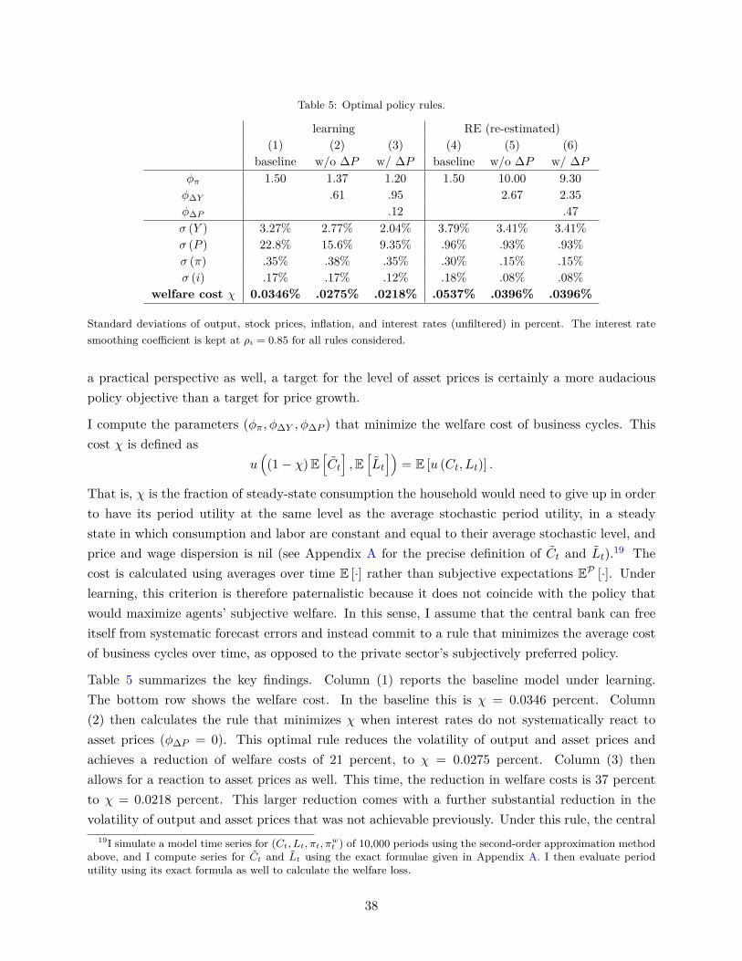
Table 5: Optimal policy rules.

learning RE (re-estimated)(1) (2) (3) (4) (5) (6)

baseline w/o ∆P w/ ∆P baseline w/o ∆P w/ ∆Pφπ 1.50 1.37 1.20 1.50 10.00 9.30φ∆Y .61 .95 2.67 2.35φ∆P .12 .47σ (Y ) 3.27% 2.77% 2.04% 3.79% 3.41% 3.41%σ (P ) 22.8% 15.6% 9.35% .96% .93% .93%σ (π) .35% .38% .35% .30% .15% .15%σ (i) .17% .17% .12% .18% .08% .08%

welfare cost χ 0.0346% .0275% .0218% .0537% .0396% .0396%

Standard deviations of output, stock prices, inflation, and interest rates (unfiltered) in percent. The interest ratesmoothing coefficient is kept at ρi = 0.85 for all rules considered.

a practical perspective as well, a target for the level of asset prices is certainly a more audaciouspolicy objective than a target for price growth.

I compute the parameters (φπ, φ∆Y , φ∆P ) that minimize the welfare cost of business cycles. Thiscost χ is defined as

u((1− χ)E

[Ct],E[Lt])

= E [u (Ct, Lt)] .

That is, χ is the fraction of steady-state consumption the household would need to give up in orderto have its period utility at the same level as the average stochastic period utility, in a steadystate in which consumption and labor are constant and equal to their average stochastic level, andprice and wage dispersion is nil (see Appendix A for the precise definition of Ct and Lt).19 Thecost is calculated using averages over time E [·] rather than subjective expectations EP [·]. Underlearning, this criterion is therefore paternalistic because it does not coincide with the policy thatwould maximize agents’ subjective welfare. In this sense, I assume that the central bank can freeitself from systematic forecast errors and instead commit to a rule that minimizes the average costof business cycles over time, as opposed to the private sector’s subjectively preferred policy.

Table 5 summarizes the key findings. Column (1) reports the baseline model under learning.The bottom row shows the welfare cost. In the baseline this is χ = 0.0346 percent. Column(2) then calculates the rule that minimizes χ when interest rates do not systematically react toasset prices (φ∆P = 0). This optimal rule reduces the volatility of output and asset prices andachieves a reduction of welfare costs of 21 percent, to χ = 0.0275 percent. Column (3) thenallows for a reaction to asset prices as well. This time, the reduction in welfare costs is 37 percentto χ = 0.0218 percent. This larger reduction comes with a further substantial reduction in thevolatility of output and asset prices that was not achievable previously. Under this rule, the central

19I simulate a model time series for (Ct, Lt, πt, πwt ) of 10,000 periods using the second-order approximation methodabove, and I compute series for Ct and Lt using the exact formulae given in Appendix A. I then evaluate periodutility using its exact formula as well to calculate the welfare loss.

38

bank raises its interest rate target 12 basis points when annualised quarterly stock price growthincreases 1 percentage point. With the interest rate smoothing parameter ρi = 0.85 this implies animmediate increase of 1.8 basis points. These numbers are not as small as it might look given thehigh volatility of stock prices. When (non-annualized) quarterly growth of the S&P500 droppedfrom -10 percent in 2008Q3 to -25.7 percent 2008Q4 at the height of the financial crisis, the rule inColumn (3) would have called for an immediate reduction in interest rates of 113 basis points fromthe stock market movement alone.

One critique of “leaning against the wind” policies is that they would lead to excessively volatileinterest rate policies. Here, the opposite is true. Despite the reaction of interest rates to stock pricesin Column (3), the volatility of interest rates drops from 0.17 percent to 0.12 percent. The reason isthat the asset price reaction greatly stabilizes equilibrium asset prices. Since investors’ subjectiveexpectations are formed on the basis of observations of past price growth, raising interest rateswhen price growth is high stabilizes these expectations at the right moment and reduces volatility.

While a reaction to asset prices is desirable under learning, the same is not true under rationalexpectations. This is shown on the right side of Table 5 which evaluates policies in the model withrational expectations, re-estimated to fit the data as discussed above. At the baseline policy inColumn (4), the welfare cost is χ = 0.0537 percent.20 This cost can be reduced by 26 percentto χ = 0.0396 percent in Column (5) under the optimal rule without a reaction to asset prices.The optimal rule reacts much more strongly to inflation than under learning and manages toconsiderably reduce inflation volatility while having little effect on the volatility of output andasset prices. When I calculate the optimal rule allowing for a non-zero φ∆P in Column (6), I dofind a positive coefficient. But the allocations obtained under this rule are almost identical to thosein Column (5) and the welfare cost is virtually unchanged. In other words, the objective functionis flat at the optimum and a rule that leans against the wind is as good as one that doesn’t. Thisresult mirrors the findings of the existing literature. As it turns out, it crucially depends on theassumption of rational expectations.

7 Conclusion

In this paper, I analyzed the implications of a learning-based asset pricing theory in a business cyclemodel with financial frictions. When firms borrow against the market value of their assets, learningin the stock market interacts with credit frictions to form a two-sided feedback loop between stockprices and firm profits that amplifies the learning dynamics encountered in Adam, Beutel, andMarcet (2014). At the same time, it leads to a large amount of propagation and amplification ofboth supply and demand shocks, while matching standard business cycle statistics and a numberof asset price properties such as the volatility, predictability, skewness and excess kurtosis of stockreturns.

20Since the model is re-estimated and does not match the data moments in the same way, the baseline welfare costunder learning and rational expectations cannot be easily compared.

39

An important innovation in developing the model was to introduce a belief system that combineslearning about asset prices with a high degree of rationality and internal consistency. Beliefs aboutvariables other than asset prices are restricted to be such that forecast errors conditional on futureprices and fundamentals are zero. This is different from rational expectations where forecast errorsconditional on fundamentals alone are zero. But it is also different from the existing adaptivelearning literature which usually parametrizes every forward-looking equation separately, resultingin a large number of degrees of freedom in specifying beliefs. The method can be widely applied inother models of the business cycle. Here, it led to forecast error predictability that closely matchessurvey data on expectations on a range of variables, despite the fact that learning only takes placeabout asset prices.

The model was also used to study normative implications of learning. In particular, I have revisitedthe question of whether monetary policy should react systematically to asset prices. I found thata reaction to stock price growth is desirable from a welfare perspective when investors in financialmarkets are learning. In contrast, under rational expectations, such a reaction does not improvewelfare, in line with previous findings in the literature. These normative findings are certainly onlya first step, but they illustrate that the choice of an asset pricing theory can have profound policyimplications.

References

Adam, K., J. Beutel, and A. Marcet (2014): “Stock Price Booms and Expected CapitalGains,” Working paper.

Adam, K., P. Kuang, and A. Marcet (2012): “House Price Booms and the Current Account,”NBER Macroeconomics Annual, 26(1), 77–122.

Adam, K., and A. Marcet (2011): “Internal rationality, imperfect market knowledge and assetprices,” Journal of Economic Theory, 146(3), 1224–1252.

Adam, K., A. Marcet, and J. P. Nicolini (2015): “Stock Market Volatility and Learning,”Journal of Finance.

Ajello, A. (2016): “Financial intermediation, investment dynamics and business cycle fluctua-tions,” American Economic Review, (forthcoming).

Altman, E. I. (2014): “The Role of Distressed Debt Markets, Hedge Funds and Recent Trends inBankruptcy on the Outcomes of Chapter 11 Reorganizations,” American Bankruptcy InstituteLaw Review, 22(1), 75–267.

Bansal, R., and A. Yaron (2004): “Risks for the Long Run: A Potential Resolution of AssetPricing Puzzles,” Journal of Finance, 59(4), 1481–1509.

40

Bernanke, B. S., and M. Gertler (2001): “Should Central Banks Respond to Movements inAsset Prices?,” American Economic Review, 91(2), 253–257.

Bernanke, B. S., M. Gertler, and S. Gilchrist (1999): “The financial accelerator in aquantitative business cycle framework,” in Handbook of Macroeconomics, ed. by J. B. Taylor, andM. Woodford, vol. 1, chap. 21, pp. 1341–1393. Elsevier.

Boldrin, M., L. J. Christiano, and J. D. M. Fisher (2001): “Habit Persistence, AssetReturns, and the Business Cycle,” American Economic Review, 91(1), pp.149–166.

Campbell, J. Y., and J. H. Cochrane (1999): “By Force of Habit: A Consumption-BasedExplanation of Aggregate Stock Market Behavior,” Journal of Political Economy, 107(2), 205–251.

Campbell, J. Y., and L. Hentschel (1992): “No news is good news,” Journal of FinancialEconomics, 31(3), 281 – 318.

Caputo, R., J. P. Medina, and C. Soto (2010): “The Financial Accelerator Under Learningand The Role of Monetary Policy,” Working Papers of the Central Bank of Chile 590, CentralBank of Chile.

Coibion, O., and Y. Gorodnichenko (2015): “Information Rigidity and the Expectations For-mation Process: A Simple Framework and New Facts,” American Economic Review, 105(8),2644–2678.

Cordoba, J.-C., and M. Ripoll (2004): International Economic Review45(4), 1011–1046.

Croce, M. M. (2014): “Long-run productivity risk: A new hope for production-based assetpricing?,” Journal of Monetary Economics, 66(0), 13–31.

Epstein, L. G., E. Farhi, and T. Strzalecki (2013): “How Much Would You Pay to ResolveLong-Run Risk?,” Working Paper 19541, NBER.

Faia, E., and T. Monacelli (2007): “Optimal interest rate rules, asset prices, and credit fric-tions,” Journal of Economic Dynamics and Control, 31(10), 3228–3254.

Fama, E. F., and K. R. French (1988): “Dividend yields and expected stock returns,” Journalof Financial Economics, 22(1), 3–25.

Flynn, E., and P. Crewson (2009): “Chapter 11 Filing Trends in History and Today,” AmericanBankruptcy Institute Journal, 14, 65 ff.

Gali, J. (2014): “Monetary Policy and Rational Asset Price Bubbles,” American Economic Review,104(3), 721–752.

41

Gelain, P., K. J. Lansing, and C. Mendicino (2013): “House Prices, Credit Growth, andExcess Volatility: Implications for Monetary and Macroprudential Policy,” International Journalof Central Banking, 9(2), 219–276.

Greenwood, R., and A. Shleifer (2014): “Expectations of Returns and Expected Returns,”Review of Financial Studies, 27(3), 714–746.

Iacoviello, M. (2005): “House Prices, Borrowing Constraints, and Monetary Policy in the Busi-ness Cycle,” American Economic Review, 95(3), 739–764.

Kobayashi, K., and K. Nutahara (2010): “Nominal Rigidities, News-Driven Business Cycles,and Monetary Policy,” B.E. Journal of Macroeconomics, 10(1), 1–26.

Lawton, A. (2012): “Chapter 11 Triage: Diagnosing a Debtor’s Prospects for Success,” ArizonaLaw Review, 54(4), 985–1028.

Lettau, M., and H. Uhlig (2000): “Can Habit Formation Be Reconciled with Business CycleFacts?,” Review of Economic Dynamics, 3(1), 79–99.

Liu, Z., P. Wang, and T. Zha (2013): “Land-Price Dynamics and Macroeconomic Fluctuations,”Econometrica, 81(3), 1147–1184.

Maussner, A. (2010): “The Analytics of New Keynesian Phillips Curves,” Discussion Paper Series313, Universitaet Augsburg, Institute for Economics.

Milani, F. (2011): “Expectation Shocks and Learning as Drivers of the Business Cycle,” EconomicJournal, 121(552), 379–401.

Sargent, T. J. (2008): “Rational Expectations,” in The Concise Encyclopedia of Economics, ed.by D. R. Henderson. Library of Economics and Liberty, 2nd edn.

Schmitt-Grohe, S., and M. Uribe (2004): “Solving dynamic general equilibrium models using asecond-order approximation to the policy function,” Journal of Economic Dynamics and Control,28(4), 755–775.

Shiller, R. (1981): “Do Stock Prices Move Too Much to be Justified by Subsequent Changes inDividends?,” American Economic Review, 71(3), 421–436.

Tallarini Jr., T. D. (2000): “Risk-sensitive real business cycles,” Journal of Monetary Eco-nomics, 45(3), 507–532.

Warren, E., and J. L. Westbrook (2009): “The Success of Chapter 11: A Challenge to theCritics,” Michigan Law Review, 107(4), 604–641.

Xu, Z., P. Wang, and J. Miao (2013): “A Bayesian DSGE Model of Stock Market Bubbles andBusiness Cycles,” Meeting Paper 167, Society for Economic Dynamics.

42

A Further details on the full model

Retailers

Retailers transform a homogeneous intermediate good into differentiated final consumption goodsusing a one-for-one technology. The intermediate good trades in a competitive market at the realprice qt (expressed in units of the composite final good). Each retailer enjoys market power inher output market, though, and sets a nominal price pit for her production. A standard priceadjustment friction à la Calvo means that a retailer cannot adjust her price with probability κ,which is independent across retailers and across time. Hence, the retailer solves the followingoptimization:

maxPit

∞∑s=0

(s∏

τ=1κΛt+τ

)((1 + τ)Pit − qt+sPt+s)Yit+s

s.t. Yit =(PitPt

)−σYt

where Qt,t+s is the nominal discount factor of households between time t and t + s, and Yt isaggregate demand for the composite final good. Since all retailers that can re-optimize at t areidentical, they all choose the same price Pit = P ∗t . Since I want to evaluate welfare in the model,I cannot log-linearize the first-order conditions of this problem. Their derivation is neverthelessstandard (for example, Maussner, 2010) and I only report the final equations here:

P ∗tPt

= 11 + τ

σ

σ − 1Γ1tΓ2t

(A.1)

Γ1t = qt + κEPt Λt+1Yt+1

Ytπσt+1 (A.2)

Γ2t = 1 + κEPt Λt+1Yt+1

Ytπσ−1t+1 (A.3)

I assume that the government sets subsidies such that τ = 1/(σ−1) so that the steady-state markupover marginal cost is zero. Inflation and the reset price are linked through the price aggregationequation which can be written as

1 = (1− κ)(P ∗tPt

)1−σ+ κπσ−1

t (A.4)

and the Tak-Yun distortion term is

∆t = (1− κ)(Γ1t

Γ2t

)−σ+ κπσt ∆t−1. (A.5)

This term ∆t ≥ 1 is the wedge due to price distortions between the amount of intermediate goodsproduced and the amount of the final good consumed. The amount of final goods available forconsumption and investment is Yt = Yt/∆t. Similarly, one can define Ct = Ct/∆t as the level of

43

consumption the household could obtain if price distortions were zero.

Labor agencies

Similarly to retailers, labor agencies transform the homogeneous household labor input into differ-entiated labor goods at the nominal price wtPt and sell them to intermediate firms at the priceWht,which cannot be adjusted with probability κw. Labor agency h solves the following optimization:

maxWht

EPt∞∑s=0

(s∏

τ=1κwΛt+τ

)((1 + τw)Wht − wt+sPt+s)Lht+s

s.t. Lht =(Wht

Wt

)−σwLt

Since all labor agencies that can re-optimize at t are identical, they all choose the same priceWht = W ∗t . The first-order conditions are analogous to those for retailers. Again, I assume thatthe government sets taxes such that τ = 1/(σw− 1) so that the steady-state markup over marginalcost is zero. Wage inflation πwt and the Tak-Yun distortion ∆wt are defined in the same way as forretailers. Finally, the real wage that intermediate producers effectively pay is

wt = Wt

Pt= wt−1

πwtπt. (A.6)

Capital good producers

Capital good producers operate competitively in input and output markets, producing new capitalgoods using old final consumption goods. For the latter, they have a CES aggregator just likehouseholds. Their maximization program is entirely intratemporal:

maxIt

QtIt −(It + ψ

2

(ItIt−1

− 1)2)

In particular, they take past investment levels It−1 as given when choosing current investmentoutput. Their first-order condition defines the price for capital goods:

Qt = 1 + ψ

(ItIt−1

− 1)

(A.7)

44

Market clearing

The market clearing conditions are summarized below. Supply stands on the left-hand side, demandon the right-hand side.

Yt =ˆ 1

0Yjtdj =

ˆ 1

0Yitdi (A.8)

Yt = Yt∆t

= Ct + It +−ψ2

(ItIt−1

− 1)2

+ Cet (A.9)

Lt =ˆ 1

0Lhtdh (A.10)

Lt = Lt∆wt

=ˆ 1

0Ljtdj (A.11)

Kt =ˆ 1

0Kjtdj = (1− δ)Kt−1 + It (A.12)

1 = Sjt, j ∈ [0, 1] (A.13)

0 = Bgt (A.14)

B Properties of the rational expectations equilibrium

The rational expectations equilibrium considered here has the following properties that need to beverified. All statements are local in the sense that for each of them, there exists a neighborhood ofthe non-stochastic steady-state in which the statement holds.

1. All firms choose the same capital-labor ratio Kjt/Ljt .

2. The expected return on capital is higher than the internal return on debt: EtRkt+1 > Rt.

3. At any time t, the stock market valuation Pjt of a firm j is proportional to its net worth afterentry and exit Njt with a slope that is strictly greater than one.

4. Borrowers never default on the equilibrium path and borrow at the risk-free rate, and thelender only accepts debt payments up to a certain limit.

5. If the firm defaults and the lender seizes the firm, it always prefers restructuring to liquidation.

6. The firm always exhausts the borrowing limit.

7. All firms can be aggregated. Aggregate debt, capital and net worth are sufficient to describethe intermediate goods sector.

I take the following steps to prove the existence of this equilibrium. After setting up the firm valuefunctions, Property 1 just follows from constant returns to scale. I then take Properties 2 and 3 asgiven and prove 4 to 6. I verify that 3 holds. The aggregation property 7 is then easily verified. Iconclude by establishing the parameter restrictions for which 2 holds.

45

Value functions

An operating firm j enters period t with a predetermined stock of capital and debt. It is convenientto decompose its value function into two stages. The first stage is given by:

Υ1 (K,B) = maxN,L,D

γN + (1− γ) (D + Υ2 (N −D))

s.t. N = qY − wL+ (1− δ)QK −RB

Y = Kα (AL)1−α

D = ζ (N −QK +B)

(I suppress the time and firm indices for the sake of notation.) After production, the firm exitswith probability γ and pays out all net worth as dividends. The second stage of the value functionconsists in choosing debt and capital levels as well as a strategy in the default game:

Υ2(N)

= maxK′,B′,strategy in default game

βE[Υ1(K ′, B′

), no default

]+ βE

[Υ1(K ′, B∗

),debt renegotiated

]+ βE [0, lender seizes firm]

s.t. K ′ = N +B′

A firm that only enters in the current period starts directly with an exogenous net worth endowmentand the value function Υ2.

Characterizing the first stage

The first order conditions for the first stage with respect to L equalizes the wage with the marginalrevenue: w = q (1− α) (K/L)αA1−α. Since there is no firm heterogeneity apart from capital K anddebt B, this already implies Property 1 that all firms choose the same capital-labor ratio. Hencethe internal rate of return on capital is common across firms:

Rk = αq

((1− α) qA

w

) 1−αα

+ (1− δ)Q (B.1)

Taking Property 3 as given for now, Υ2 is a linear function with slope strictly greater than one.

46

Then the following holds for the first-stage value function Υ1:

Υ1 (K,B) = N + (1− γ) (D −N + Υ2 (N −D))

= N + (1− γ)(Υ ′2 − 1

)((1− ζ)N + ζ (QK −B))

> N

= RkK −RB (B.2)

This property will be used repeatedly in the next step of the proof.

Characterizing the second stage

The second stage involves solving for the subgame-perfect equilibrium of the default game betweenborrower and lender. Pairings are anonymous, so repeated interactions are ruled out. Also, onlythe size B and the interest rate R of the loan can be contracted (I omit primes for ease of notationand separate R from the risk-free rate R). The game is played sequentially:

1. The firm (F) proposes a borrowing contract(B, R

).

2. The lender (L) can accept or reject the contract.

• A rejection corresponds to setting the contract(B, R

)= (0, 0).

Payoff for L: 0. Payoff for F: βE[Υ1(N , 0

)].

3. F acquires capital and can then choose to default or not.

• If F does not default, it has to repay in the next period.Payoff for L: EQt,t+1RB −B. Payoff for F: βE

[Υ1(K, RRB

)].

4. If F defaults, the debt needs to be renegotiated. F makes an offer for a new debt level B∗.21

5. L can accept or reject the offer.

• If L accepts, the new debt level replaces the old one.Payoff for L: EΛRB∗ −B. Payoff for F: βE

[Υ1(K, RRB

∗)].

6. If L rejects, then she seizes the firm. A fraction 1−ξ of the firm’s capital is lost in the process.Nature decides randomly whether the firm can be “restructured.”

• If the firm cannot be restructured, or it can but the lender chooses not to do so, thenthe lender has to liquidate the firm.Payoff for L: EΛξQK −B. Payoff for F: 0.

21That the interest rate on the repayment is fixed is without loss of generality.

47

• If the firm can be restructured and the lender chooses to do so, she retains a debt claimof present value ξB and sells the residual equity claim in the firm to another investor.Payoff for L: ξB + βE [Υ1 (ξK, ξB)]−B. Payoff for F: 0.

Backward induction leads to the (unique) subgame-perfect equilibrium of this game. Start withthe possibility of restructuring. L prefers this to liquidation if

ξB + βE [Υ1 (ξK, ξB)] ≥ EΛξQK. (B.3)

This holds true at the steady state because Rk > R (Property 2), Q = 1, β = Λ and

ξB + βE [Υ1 (ξK, ξB)] > ξB + βE[RkξK −RξB

]= βE

[RkξK

]> ξK (B.4)

Since the inequality is strict, the statement holds in a neighborhood around the steady-state aswell. This establishes Property 5.

Next, L will accept an offer B∗ if it gives her a better expected payoff (assuming that lenders candiversify among borrowers so that their discount factor is invariant to the outcome of the game).The probability of restructuring is given by x. The condition for accepting B∗ is therefore that

EΛRB∗ ≥ x(ξB + βE [Υ1 (ξK, ξB)]

)+ (1− x)EΛξQK. (B.5)

Now turn to the firm F. Among the set of offers B∗ that are accepted by L, the firm will prefer thelowest one—i.e., that which satisfies (B.5) with equality. This follows from Υ1 being a decreasingfunction of debt. This lowest offer will be made if it leads to a higher payoff than expropriation:βE

[Υ1(K, RRB

∗)]≥ 0. Otherwise, F offers zero and L seizes the firm.

Going one more step backwards, F has to decide whether to declare default or not. It is preferableto do so if the B∗ that L will just accept is strictly smaller than B or if expropriation is better thanrepaying, βE

[Υ1(K, RRB

)]≥ 0.

What is then the set of contracts that L accepts in the first place? From the perspective of L, thereare two types of contracts: those that will not be defaulted on and those that will. If F does notdefault (B∗ ≥ B), L will accept the contract simply if it pays at least the risk-free rate, R ≥ R. IfF does default (B∗ < B), then L accepts if the expected discounted recovery value exceeds the sizeof the loan—i.e., EΛRB∗ ≥ B.

Finally, let us consider the contract offer. F can offer a contract on which it will not default. Inthis case, it is optimal to offer just the risk-free rate R = R. Also note that the payoff from this

48

strategy is strictly positive since

βE [Υ1 (K,B)] > βE[RkK −RB

]= βE

[RkN +

(Rk −R

)B]

> 0. (B.6)

The payoff is also increasing in the size of the loan B. So conditional on not defaulting, it isoptimal for F to take out the maximum loan size B = B∗, and this is preferable to default withexpropriation. However, it might also be possible for F to offer a contract that only leads to adefault with debt renegotiation. The optimal contract of this type is the solution to the followingproblem:

maxR,B,B∗

βE[Υ1

(N +B,

R

RB∗)]

s.t. EΛRB∗ ≥ B

EΛRB∗ = x(ξB + βE

[Υ1(ξ(N +B

), ξB

)])+ (1− x)EΛQξ

(N +B

)The first thing to note is that only the product RB∗ appears, so the choice of the interest rate R isredundant. Further, B = B∗ and R = R solve this problem, and this amounts to the same as notdeclaring default. This choice solves the maximization problem above if the following condition issatisfied at the steady state:

ξ

R

(1− x+ xR+ xΥ ′1

[Rk

R− 1

])< 1 (B.7)

For the degree of stock price dependence x sufficiently small, this condition is satisfied. Thisestablishes Properties 4 and 6.

Linearity of firm value

Since firms do not default and exhaust the borrowing limit B∗, the second-stage firm value can bewritten as follows:

Υ2(N)

= βE[Υ1(N +B,B

)](B.8)

where B = x(ξB + βE

[Υ1(ξ(N +B

), ξB

)])+ (1− x)Qtξ

(N +B

)(B.9)

We already know that if Υ2 is a linear function, then Υ1 is also linear. The converse also holds: Theconstraint above, together with linearity of Υ1 imply that B is linear in N , and thus Υ2 is linear,too.

49

To establish Property 3, it remains to show that the slope of Υ2 is greater than one. This is easyto see in steady state:

Υ ′2 = βΥ1 (K,B)

N

= βγ(RkK −RB

)+ (1− γ)Υ2

(RkK −RB

)N

= β(γ + (1− γ)Υ ′2

) (Rk

K

N−RB

N

)

=(γ + (1− γ)Υ ′2

) Rk +(Rk −R

)BN

R︸ ︷︷ ︸=:c0>1

= γc01− (1− γ) c0

> 1 (B.10)

Finally, the aggregated law of motion for capital and net worth needs to be established (Property7). Denoting again by Γt ⊂ [0, 1] the indices of firms that exit and are replaced in period t, we have

Kt =ˆ 1

0Kjtdj =

ˆj /∈Γt

(Njt − ζEjt +Bjt) dj +ˆj∈Γt

(ω (Nt − ζEt) +Bjt) dj

= (1− γ + γω) (Nt − ζEt) +Bt (B.11)

Nt =ˆ 1

0Njtdj = RktKt−1 −Rt−1Bt−1 (B.12)

Bt =ˆ 1

0Bjtdj = xξ (Bt + Pt) + (1− x) ξEtΛt+1Qt+1Kt (B.13)

So far, then, all model properties are established except for Rk > R.

Return on capital

It can now be shown under which conditions the internal rate of return is indeed greater than thereturn on debt. From the steady-state versions of equations (B.11) and (B.12), it follows that

Rk = R+ (G−R (1− γ + γω)) NK

+Rc (1− γ + γω) EK. (B.14)

Sufficient conditions for Rk > R are therefore that N/K and E/K are strictly positive and thatthe following holds:

γ >R−G

G (1− ω) . (B.15)

50

C Approximation method for the learning equilibrium

The second-order perturbation method for the learning equilibrium follows Schmitt-Grohe andUribe (2004) but has to be adapted to allow for relaxation of the rational expectations assumption.A rational expectations equilibrium can generally be described as a solution (yt)t∈N to

Et [f (yt+1, yt, xt, ut)] = 0, (C.1)

where Et is the expectations operator with respect to the probability measure and filtration inducedby exogenous stochastic disturbances ut. These disturbances are of dimensionality nu, independentand identically distributed, of zero mean and variance σ2Σu. The solution yt is of dimensionality n,as is the image of f . xt denotes a vector of predetermined state variables of dimensionality nx < n:xi,t = yι(i),t−1 for an injective ι : {1..n} → {1..nx}, or simply xt = Cyt−1 for an appropriate matrixC. One is interested in finding a policy function that generates solutions of the form

yt = g (xt, ut, σ) . (C.2)

Perturbation methods for approximating the policy function to higher orders are straightforward.They compute Taylor expansions of g, typically around a non-stochastic steady state of the model:a constant solution y for σ = 0 such that f (y, y, x, 0) = 0 and hence g (y, 0, 0) = y.

In a learning equilibrium, (C.1) does not fully characterize the equilibrium because the probabilitymeasure used by agents to form expectations does not coincide with the actual probability measureof the model. The stock price in the model of this paper is determined by the usual market-clearing condition, but agents think it is determined by random unpredictable shocks that are notnecessarily related to the rest of the economy. A model described by (C.1) cannot contain a shockthat is perceived as exogenous but at the same time is determined endogenously.

The model in this paper belongs to a class that can be written as follows:

EPt [f (yt+1, yt, xt, ut, zt)] = 0 (C.3)

EPt [φ (yt+1, yt, xt, ut, zt)] = 0 (C.4)

Here, the probability measure P denotes beliefs for which the disturbances zt (of dimensionality nz)are perceived as exogenous, independent, and identically distributed with zero mean and varianceσ2Σz. They are also perceived as independent of ut, although this can be relaxed. These distur-bances have the interpretation of forecast errors. The iid assumption then amounts to imposingthat agents holding the belief P think their forecasts cannot be improved upon. As before, f is ofdimensionality n. The system (C.3) is assumed to have a unique solution for each initial conditionxt and path of disturbances ut and zt which can be described by a subjective policy function:

yt = h (xt, ut, zt, σ) (C.5)

51

Contrary to agents’ beliefs, zt is not an exogenous disturbance but is determined endogenouslyby the second set of equilibrium conditions (C.4). The function φ is of dimension nz. This setof conditions is not known to agents. The actual probability measure P0, induced by (C.3)–(C.4)and the disturbances ut, is thus different from P. Under P0, zt is a function of the state and thefundamental disturbances:

zt = r (xt, ut, σ) (C.6)

This leads to the objective policy function:

g (xt, ut, σ) = h (xt, ut, r (xt, ut, σ) , σ) (C.7)

All functional forms are assumed to be such that the functions h and r are uniquely determined.

In the case of the model of this paper, lagged belief updating requires two pseudo-disturbances,nz = 2. Agents cannot update their beliefs about future stock prices at the same time as theyobserve current prices, yet by observing the price they can infer the current forecast error. Thisimplies the following subjective belief equations that are part of (C.3):

logPt = logPt−1 + µt −σ2η + σ2

ν

2 + z1t (C.8)

µt = µt−1 −σ2ν

2 + gz2t (C.9)

The conditions (C.4) that pin down the values for the forecast errors zt in equilibrium are thendescribed as follows:

Pt − βEPt [Dt+1 + Pt+1] = 0 (C.10)

z2t − z1t−1 = 0 (C.11)

Going back to the general case, the goal is to derive an accurate second-order approximation of theobjective policy function g around the non-stochastic steady state:

g (xt, ut, σ) ≈ g (x, 0, 0)

+ gx (xt − x) + guut + gσσ

+ 12gxx [(xt − x)⊗ (xt − x)] + 1

2gxu [(xt − x)⊗ ut] + 12guu [ut ⊗ ut]

+ 12gσσσ

2 (C.12)

The first step in deriving the approximation is calculating this approximation for the subjectivepolicy function h. This can be done using standard methods as implemented in Dynare. Thesecond step is finding the derivatives of the function r in (C.6). Substituting it into the equilibrium

52

conditions (C.4) gives

0 = Φ (x, u, σ) = EPt[φ(y′, y, x, u, z

)]= EPt

φ h (Ch (x, u, z, σ) , u′, z′, σ) ,

h (x, u, z, σ) , x, u, z

= EPt

φ h (Ch (x, u, r (x, u, σ) , σ) , u′, z′, σ) ,h (x, u, r (x, u, σ) , σ) , x, u, r (x, u, σ)

. (C.13)

Here, I drop time subscripts and denote by prime variables at t+1. Note that the term z′ must notbe substituted out when the expectation is taken under P. Doing so would imply that agents knowthe true relationship between zt+1 and the model variables instead of taking it as an exogenousdisturbance. Total differentiation at the non-stochastic steady state leads to the following first-orderderivatives:

0 = dΦdx

(x, 0, 0) =(φy′hxC + φy

)(hx + hzrx) + φx + φzrx (C.14)

0 = dΦdu

(x, 0, 0) =(φy′hxC + φy

)(hu + hzru) + φu + φzru (C.15)

0 = dΦdσ

(x, 0, 0) =(φy′hxC + φy

)(hσ + hzrσ) + φzrσ (C.16)

Since the existence of a unique solution for r is assumed, the first derivatives can be solved for. Ialso assume that the equilibrium conditions imply that z = 0 at the steady state. This means thatin the absence of shocks, agents make no forecast errors under learning.

Define the matrix A =(φy′hxC + φy

)hz + φz. Then the first-order derivatives of r are given by

rx = −A−1 ((φy′hxC + φy)hx + φx

)(C.17)

ru = −A−1 ((φy′hxC + φy)hu + φu

)(C.18)

rσ = 0. (C.19)

Up to first order, the existence and uniqueness of the function r is equivalent to invertibility of thematrix A. The first-order derivatives of the actual policy function g can be obtained by applyingthe chain rule. The certainty-equivalence property holds for the subjective policy function h, hencehσ = 0. This implies that rσ = 0 and gσ = 0 as well, so certainty equivalence also holds underlearning.

The second-order calculations are similar, if more tedious. The second-order derivative of Φ with

53

respect to x is

0 = d2Φdx2 (x, 0, 0) =

(φy′gxC + φy

)(hxx + 2hxz [Inx ⊗ rx] + hzz [rx ⊗ rx])

+ φy′hxx [Cgx ⊗ Cgx] +Bxx +Arxx. (C.20)

This equation isn2x-dimensional and linear in rxx and thus can be solved easily. As in first order,

only invertibility of the matrix A is required for a unique local solution under learning. I havecollected all cross-derivatives of φ inside the matrix Bxx (of size nz × n2

x), which contains onlyfirst-order derivatives of the policy functions:

Bxx = φy′y′ [hxCgx ⊗ hxCgx] + φyy [gx ⊗ gx] + φxx + φzz [rx ⊗ rx]

+ 2φy′y [hxCgx ⊗ gx] + 2φy′x [hxCgx ⊗ Inx ] + 2φy′z [hxCgx ⊗ rx]

+ 2φyx [gx ⊗ Inx ] + 2φyz [gx ⊗ rx] + 2φxz [Inx ⊗ rx] (C.21)

The formulae to solve for rxu and ruu are analogous. It remains to look at the derivatives involvingσ. This simplifies considerably because the first derivatives of the policy functions g and h withrespect to σ are zero. The cross-derivative of Φ with respect to x and σ thus reads:

0 = d2Φdxdσ

(x, 0, 0) =(φy′gxC + φy

)(hxσ + hzrxσ) + φzrxσ (C.22)

But because hxσ = 0, as under rational expectations, rxσ = 0 holds as well. The same applies toruσ = 0. Finally, the second derivative with respect to σ involves the variance of the disturbances:

0 = d2Φdσ2 (x, 0, 0) = φy′y′ (hσσ + huuvec (Σu) + +hxxvec (Σz))

+ φy′y′(vec

(h′uΣuhu

)+ vec

(h′zΣzhz

))+

(φy′gxC + φy

)(hσσ) +Arσσ (C.23)

Again, this can be solved for rσσ when A is invertible. Note that the perceived variance Σz appearsin the calculation because it matters for expectations for the future (unless φy′y′ = 0). This varianceis not necessarily equal to the objective variance of z.

The second-order derivatives of the actual policy function g are calculated easily once those of rare known:

gxx = hxx + 2hxz [Inx ⊗ rx] + gzz [rx ⊗ rx] + gzrxx (C.24)

and analogously for gxu, guu and gσσ. The cross-derivatives guσ and gxσ are zero.

54