Asset Prices and Institutional Investors∗

Suleyman Basak Anna Pavlova

London Business School London Business School

and CEPR and CEPR

This version: August 2012

Abstract

Empirical evidence indicates that trades by institutional investors have sizable effects onasset prices, generating phenomena such as index effects, asset-class effects and others. Itis difficult to explain such phenomena within standard representative-agent asset pricingmodels. In this paper, we consider an economy populated by institutional investors alongsidestandard retail investors. Institutions care about their performance relative to a certainindex. Our framework is tractable, admitting exact closed-form expressions, and producesthe following analytical results. We find that institutions optimally tilt their portfoliostowards stocks that comprise their benchmark index. The resulting price pressure boostsindex stocks, while leaving nonindex stocks unaffected. By demanding a higher fractionof risky stocks than retail investors, institutions amplify the index stock volatilities andaggregate stock market volatility, and give rise to countercyclical Sharpe ratios. Trades byinstitutions induce excess correlations among stocks that belong to their benchmark index,generating an asset-class effect.

JEL Classifications: G12, G18, G29Keywords: Asset pricing, indexing, institutions, money management, general equilibrium.

∗Email addresses: sbasak@london.edu and apavlova@london.edu. We have benefitted from valuable feed-back of Patrick Bolton, Georgy Chabakauri, Guillaume Plantin, Raman Uppal, Dimitri Vayanos, our col-leagues at LBS, our discussants Julien Hugonnier, Ron Kaniel, Ralph Koijen, Lukas Schmid, and threeanonymous referees, as well as seminar participants at the Bank of Italy, Carlo Alberto, Chicago Booth,CBS, Erasmus, HEC Paris, IDC Herzliya, IE, Koc, Lancaster, LBS, LSE, St. Gallen, Stockholm, USC, War-wick, Zurich, and the 2011 AFA, CRETE, and EFA meetings, ESSET 2011 at Gerzensee, ICBFP conference,Paul Woolley Centre conference, and Swissquote conference for helpful comments and Federica Pievani forexcellent research assistance. Pavlova thanks the European Research Council for financial support (GrantERC263312).

1. Introduction

A significant part of the trading volume in financial markets is attributed to institutional

investors. Trades by retail investors constitute only a small fraction of the trading volume.1

In contrast, the standard theories of asset pricing stipulate that prices in financial markets are

determined by households (or by the “representative consumer” aggregated over households)

who seek to optimize their consumption and investment over their life cycle. This approach

leaves no role for important considerations influencing institutional investors’ portfolios such

as, for instance, compensation-induced incentives or implicit incentives arising from the

predictability of inflows of capital into the money management business. This underscores

the importance of studying how the incentives of institutional investors may influence the

prices of the assets they hold.

In this paper, we take institutional investors to be institutional/professional asset man-

agers. These managers have a mandate to manage a portfolio for a mutual fund, a hedge

fund, a pension fund, an endowment, an asset management team in a bank or insurance com-

pany, etc. In our analysis, we focus on perhaps the most prominent feature of professional

managers’ incentives: concern about own performance vis-a-vis some benchmark index (e.g.,

S&P 500). This characteristic is what induces institutional investors to act differently from

retail investors. Relative performance matters because inflows of new money into institu-

tional portfolios and payouts to asset managers at year-end depend on it, or simply because

managers care about their standing in the profession (status). Our goal is to demonstrate

how, in the presence of such incentives, institutions optimally tilt their portfolios towards

the stocks in their benchmark index, influencing the performance of the index, and in the

process how they exacerbate leverage in the economy as well as stock market volatility, and

boost the correlation among the stocks that are included in the index.

We consider a dynamic general equilibrium model with two classes of investors: “re-

tail” investors with standard logarithmic preferences and “institutional” investors who are

concerned not only about their own performance but also about the performance of a bench-

mark index. The institutional investors have an additional incentive to post a higher return

1See, for example, Griffin, Harris, and Topaloglu (2003).

1

when their benchmark is high than when it is low, in an effort to outdo the benchmark.

Formally, their marginal utility of wealth is increasing with the level of their benchmark

index. Towards that we take a reduced-form approach in our specification of the institu-

tional investor’s objective function that captures the above salient features and admits much

tractability. In our model, there are multiple risky stocks, some of which are part of the

index, and a riskless bond. The stocks are in positive net supply, while the bond is in zero

net supply. The model is designed to capture several important empirical phenomena and

to provide the economic mechanisms generating these phenomena. One major advantage

of our model is that it delivers exact, closed-form expressions for all quantities which are

behind our results described below.

We first examine the tilt in the portfolios of the institutional investors which is caused

by the presence of the benchmark indexing. We find that, relative to the retail investor,

the institution increases the fraction of index stocks in the portfolio so as not to fall behind

when the index does well. To finance this additional demand for index stocks, the institution

takes on leverage.2 So the institutions in our model always end up borrowing funds from the

retail sector, to the extent allowed by the size of their assets under management that serve

as collateral. As institutions continue to do well and accumulate assets, they increase the

overall leverage in the economy, but only up to a certain point determined by the lending

capacity of the retail sector.

We next investigate how the presence of institutions influences asset prices. Our first

finding is that institutions push up the prices of stocks in the benchmark index. In the econ-

omy with institutional investors, the index stock prices are higher both relative to those in

the retail-investor-only economy and relative to their (otherwise identical) nonindex coun-

terparts. This is because institutions generate excess demand for the index stocks. This

finding is well supported in the data: such an “index effect” occurs in many markets and

2Our institutions may be interpreted as mutual funds. Due to regulation, most mutual funds choose tobe long-only, although some do use leverage (e.g., the 130/30 funds). Other, less regulated, institutionalinvestors can use leverage (closed-end funds, hedge funds, etc.). We further note that leverage is inevitablein a model with heterogeneous agents and a zero-net supply riskless bond. However, it is not essential forour mechanism; what is essential is that institutions have excess demand for index stocks. In Appendix C,we present a variant of our model without leverage. In that model there are only (positive net supply) riskystocks available for trading and there is no riskless bond. Typically the investors are long in all stocks. Theyhave an excess demand for index stocks and they finance this additional demand by reducing their portfolioweights in nonindex stocks.

2

countries.3

We also find that the price pressure from the institutions boosts the level of the overall

stock market in addition to the index. This is because the institutions have a higher demand

for risky assets than retail investors. Since the stocks are in fixed supply, the index stocks

have to become less attractive for markets to clear. This translates into higher volatilities

and lower Sharpe ratios for the index stocks and the overall stock market. The presence of

institutions also induces time variation in these quantities; in particular makes Sharpe ratios

countercyclical. This is because the institutions are over-weighted in the risky assets. They

therefore benefit more from good cash flow news than retail investors, and so become more

dominant in the economy. This amplifies the cash flow news and pushes down the Sharpe

ratios. As the size of institutions increases, their influence on equilibrium also becomes more

pronounced. Therefore, the Sharpe ratios are lower in good times than in bad times. In light

of these findings, one can attempt to examine the effects on asset markets of several popular

policy recommendations put forward during the 2007-2008 financial crisis. We make no wel-

fare comparisons here; we simply highlight the side effects of some policy recommendations.

One such recommendation was to impose leverage caps on institutions, excessive leverage of

which had arguably caused the crisis. In our model, when institutions do not control the

dominant fraction of wealth in the economy, a leverage cap brings down the riskiness of their

portfolios (an intended effect) but it also brings down the level of stock prices, creating an

adverse side effect.

Finally, we examine the correlations among stocks included in the index and stocks out-

side the index. We find that the presence of institutions who care explicitly about their index

induces time-varying correlations and generates an “asset-class” effect: returns on stocks be-

longing to the index are more correlated amongst themselves than with those of otherwise

identical stocks outside the index. This asset-class effect is, of course, absent in the retail-

3Starting from Harris and Gurel (1986) and Shleifer (1986), a series of papers documents that prices ofstocks that are added to the S&P 500 and other indices increase following the announcement and prices ofstocks that are deleted drop. For example, Chen, Noronha, and Singal (2004) find that during 1989-2000,the stock price increased by an average of 5.45% on the day of the S&P 500 inclusion announcement and afurther 3.45% between the announcement and the actual addition. The corresponding figures for the S&P500 deletions are -8.46% and -5.97%, respectively. Moreover, the index effect has become stronger after 1989.While there are possible alternative explanations to this phenomenon, the growth of the institutions whobenchmark their performance against the index remains a leading one.

3

investor-only benchmark economy: there, the correlation between any two stocks’ returns

is determined simply by the correlation of their fundamentals (dividends). The additional

correlation among the index stocks is caused by the additional demand of institutions for

the index stocks: the institutions hold a hedging portfolio, consisting of only index stocks,

that hedges them against fluctuations in the index. Following a good realization of cash

flow news, institutions get wealthier and demand more shares of index stocks relative to

the retail-investor-only benchmark. This additional price pressure affects all index stocks at

the same time, inducing excess correlations among these stocks. Empirical research lends

support to our findings; asset-class effects have now been documented in many markets.4

We get the time-varying correlations in the presence of institutions for the same reasons as

for the time-varying volatilities.

It is somewhat surprising that despite extensive empirical work showing that institutions

have important effects on asset prices and despite the 2007-2008 financial crisis that has made

this point all too obvious, we still have little theoretical work on equilibrium in the presence

of professional money management. Brennan (1993) is the first to attempt to introduce

institutional investors into an asset pricing model. Brennan considers a static mean-variance

setting with constant absolute risk aversion (CARA) utility agents who are compensated

based on their performance relative to a benchmark index. He shows that in equilibrium

expected returns are given by a two-factor model, with the two factors being the market

and the index. More recent related, also static, mean-variance models appear in Gomez

and Zapatero (2003), Cornell and Roll (2005), Brennan and Li (2008), Leippold and Rohner

(2008), and Petajisto (2009). CARA utility, as is well-known, rules out wealth effects, which

play a central role in our paper.

Cuoco and Kaniel (2011) develop a dynamic equilibrium model with constant relative

risk aversion (CRRA) agents who explicitly care about an index due to performance-based

4For example, Barberis, Shleifer, and Wurgler (2005) show that when a stock is added to the S&P 500index, its beta with respect to the S&P 500 goes up while its non-S&P 500 “rest of the market” beta falls;and the opposite is true for stocks deleted from the index. Moreover, these effects are stronger in more recentdata. Boyer (2011) provides similar evidence for BARRA value and growth indices. He finds that “marginalvalue” stocks—the stocks that just switched from the growth into the value index—comove significantly morewith the value index; the opposite is true for the “marginal growth” stocks. Consistent with the institutionalexplanation for this phenomenon, Boyer finds that the effect appears only after 1992, which is when BARRAindices were introduced.

4

fees.5 In a two-stock economy, Cuoco and Kaniel show that inclusion in an index increases a

stock’s price and illustrate numerically that it also lowers its unconditional expected return

and increases its unconditional volatility. However, in an exercise more closely related to

the one we perform in this paper, they show numerically that, in contrast to our work, the

conditional volatilities of the index stock and aggregate stock market decrease in the presence

of benchmarking. In another closely related paper, He and Krishnamurthy (2012a) consider

a dynamic single-stock model with CRRA (logarithmic) institutions, in which institutions

are constrained in their portfolio choice due to contracting frictions. They show that in bad

states of the world (crises), institutional constraints are particularly severe, causing increases

in the stock’s Sharpe ratio and conditional volatility and replicating other patterns observed

during crises. This literature remains sparse due to the modeling challenges of tractably

solving for asset prices in the presence of wealth effects and multiple assets. We overcome

this challenge by modeling institutions differently: our model has the tractability of CARA-

based models but it additionally features wealth effects. This tractability not only allows

us to elucidate the mechanisms through which institutions influence asset prices, but also to

extend our setting to multiple risky stocks, permitting an analysis of the “asset-class” effect.

The closest theoretical model that exhibits the “asset-class” effect is by Barberis and Shleifer

(2003), whose explanation for this phenomenon is behavioral. By providing microfoundations

for investors’ demand schedules, we can establish a set of primitives that give rise to the

asset-class effect and discuss what these primitives imply for other equilibrium quantities

(time-varying volatilities, Sharpe ratios, leverage, risk tolerance and others). Moreover, the

correlations of stocks within an asset class in our model are time-varying due to wealth

effects.

Other related papers that have explored equilibrium effects of delegated portfolio manage-

ment include He and Krishnamurthy (2012b), in which poor performance of fund managers

triggers portfolio outflows due to contracting frictions, Dasgupta and Prat (2008), Dasgupta,

Prat, and Verardo (2008), Malliaris and Yan (2010), Vayanos and Woolley (2010), Guerreri

and Kondor (2012), in which outflows following poor performance are due to learning about

managerial ability, and Vayanos (2004) and Kaniel and Kondor (2012) in which outflows oc-

5See also Kapur and Timmermann (2005) and Arora, Ju, and Ou-Yang (2006) for related dynamic models.

5

cur for exogenous reasons, dependent on fund performance. They show that, similar to our

findings, flow-based considerations amplify the effects of exogenous shocks on asset prices.

All of these papers model various agency frictions. In our model, we simplify this aspect,

but offer a richer model of a securities market. We view these papers as complementary to

our work. Our paper is also connected to the literature on relative wealth concerns and asset

prices (Galı (1994)). For example, in DeMarzo, Kaniel, and Kremer (2004, 2008), where

such concerns arise endogenously, agents care about their relative wealth in the community

which causes them to overinvest in stocks held by other members of their community. In our

model, the institutional investors end up overinvesting in the index stocks.

Finally, there is a related literature on the effects of fund flows and benchmarking con-

siderations on portfolio choice of fund managers, at a partial equilibrium level. For example,

Carpenter (2000), Basak, Pavlova, and Shapiro (2007, 2008), Hodder and Jackwerth (2007),

Binsbergen, Brandt, and Koijen (2008), and Chen and Pennacchi (2009) show that future

fund flows induce a manager to tilt her portfolio towards stocks that belong to her benchmark.

These papers demonstrate that there is a range over which such benchmarking considera-

tions induce her to take more risk. The main difference of our paper from this body of work

is that we examine the general equilibrium effects of benchmarking.

The remainder of our paper is organized as follows. Section 2 presents a simplified

single-stock version of our model for which we establish a number of our results in the

clearest possible way. Section 3 discusses the index effect, institutional risk-taking, wealth

effects, and the resulting policy implications. Section 4 presents the general multi-stock

version of our model and focuses on the asset-class effect and Section 5 summarizes our

key predictions and empirical implications. Appendix A contains all proofs, Appendix B

generalizes the analysis to nonzero dividend growth and interest rate, Appendix C presents

the stocks-only version of our model, and Appendix D provides an agency-based justification

for the institutional objective function.

6

2. Economy with Institutional Investors

2.1. Economic Setup

We consider a simple and tractable pure-exchange security market economy with a finite

horizon. The economy evolves in continuous time and is populated by two types of market

participants: retail investors, R, and institutional investors, I. In the general specification

of our model, there are N stocks, M of which are included in the index against which the

performance of institutions is measured, as well as a riskless bond. In this section, however,

we specialize the securities market to feature a single risky stock, henceforth referred to as

the stock market index, and a riskless bond. The index is exposed to a single source of risk

represented by a Brownian motion ω. The main reason for considering the single-stock case

is expositional simplicity. It turns out that a number of key insights of this paper can be

illustrated within the single-stock economy. We then build on our baseline intuitions and

expand them (Section 4) to demonstrate how our economy behaves in the general case in

which there are multiple stocks and multiple sources of risk.

Investment opportunities. The stock market index, S, is posited to have dynamics given

by

dSt = St[µStdt+ σStdωt], (1)

with σSt > 0. The mean return µS and volatility σS are determined endogenously in equilib-

rium (Section 3). The bond is in zero net supply. It pays a riskless interest rate r, which we

set to zero without loss of generality.6 The stock market index is in positive net supply. It

is a claim to the terminal payoff (or “dividend”) DT , paid at time T , and hence ST = DT .

This payoff DT is the terminal value of the process Dt, with dynamics

dDt = Dt[µdt+ σdωt], (2)

where µ and σ > 0 are constant. The process Dt represents the arrival of news about

6This is equivalent to using the riskless bond as the numeraire and denoting all prices in terms of thisnumeraire. Such an assumption is innocuous because our model does not have intermediate consumption.In other words, there is no intertemporal choice that would pin down the interest rate. Our normalization iscommonly employed in models with no intermediate consumption (see e.g., Pastor and Veronesi (2012) fora recent reference). In Appendix B, we incorporate a nonzero (constant) interest rate. This change modifiesour formulae, but leaves our economic insights unchanged.

7

DT . We refer to it as the cash flow news. Equation (2) implies that cash flow news arrives

continuously and that DT is lognormally distributed. The lognormality assumption is made

for technical convenience. For expositional purposes, we set µ = 0, as this simplification

does not alter any of our economic insights.7

Investors. Each type of investor i = I, R in this economy dynamically chooses a portfolio

process ϕi, where ϕi denotes the fraction of the portfolio invested in the stock index, or the

risk exposure, given the initial assets of Wi0. The wealth process of investor i, Wi, then

follows the dynamics

dWit = ϕitWit[µStdt+ σStdωt]. (3)

The (representative) institutional and retail investors are initially endowed with fractions

λ ∈ [0, 1] and (1 − λ) of the stock market index, providing them with initial assets worth

WI0 = λS0 and WR0 = (1 − λ)S0, respectively.8 The parameter λ thus represents the

(initial) fraction of the institutional investors in the economy—or equivalently, how large

the institutions are relative to the overall economy. It is an important comparative statics

parameter in our analysis, which allows us to illustrate how the growth of the financial sector

(or more precisely, funds managed by institutions) can influence asset prices.

The retail investor has standard logarithmic preferences over the terminal value of her

portfolio:

uR(WRT ) = log(WRT ). (4)

In modeling the institutional investor’s objective function, we consider two noteworthy fea-

tures of the professional money management industry that make institutions behave differ-

ently from retail investors. First, institutional investors care about their benchmark index.

This can be due to implicit or explicit incentives. The implicit incentives to perform well in

relative terms come in the form of inflow/outflow of funds in response to relative performance.

7Appendix B generalizes the analysis to incorporate a nonzero dividend growth rate and demonstratesthat all our predictions remain equally valid. Moreover, in related analysis (not presented here due to spacelimitations), we relax the lognormality assumption and show that the bulk of our results remains valid formore general stochastic processes, but the characterization of our economy becomes more complex.

8We do not explicitly model households, who delegate their assets to institutions to manage, but simplyendow the institutions with an initial portfolio. The households who delegate their money to the institutionscan be thought of, for example, as participants in defined benefit pension plans (worth $3.14 trillion in theUS as of June 2009 according to official figures and significantly more according to Novy-Marx and Rauh(2010)).

8

The fee of practically any type of an institutional asset manager includes a fraction of funds

under management. Institutional asset managers therefore seek to perform well relative to

their peer group so as to attract more new funds than their less successful peers. This posi-

tive flows-performance relation is a prevalent finding in asset management, as documented by

Chevalier and Ellison (1997) and Sirri and Tufano (1998) for mutual funds, Agarwal, Daniel,

and Naik (2004) and Ding, Getmansky, Liang and Wermers (2010) for hedge funds, and

Del Guercio and Tkac (2002) for pension funds. For the purposes of highlighting explicit

incentives of fund managers, it is important to distinguish between external and internal

managers. External managers (working for e.g., large pension funds or endowments) typi-

cally have mandates that get reviewed every one to five years by the trustees. These reviews

are based to a large extent on their performance relative to passive benchmarks, and these

managers win/lose mandates as well as attract inflows based on their relative performance

(BIS (2003), p.22). With the exception of hedge funds, internal managers receive bonuses

that are linked to performance relative to their benchmarks (e.g., BIS (2003), p.23; Ma,

Tang, and Gomez (2012)). Such explicit and implicit incentives make both types of man-

agers care about their relative performance. This discussion leads us to the second feature of

professional asset management that we attempt to capture: money managers strive to post

a higher return when their benchmark is high than when it is low, in an effort to outdo their

benchmark. Putting this formally, their marginal utility of wealth is increasing in the level

of their benchmark index. This feature can also be microfounded using an agency-based

argument, following the ideas of Holmstrom (1979, 1982). In Appendix D, we employ the

approach of Edmans and Gabaix (2011) to demonstrate it formally. Accordingly, we formu-

late the institutional investor’s objective function over the terminal value of her portfolio as

being given by:

uI(WIT ) = (a+ bST ) log(WIT ), (5)

where a, b > 0. We set a = 1, since by homogeneity only the ratio b/a matters in the

ensuing analysis. In this one-stock economy, the manager’s benchmark index coincides with

the stock market.9

9The objective function then has another interpretation: the institutional investor has an incentive toperform well during bull markets (high ST ). This is plausible since empirical evidence indicates that duringbull markets payouts to money managers are especially high. For example, there are higher money inflows

9

There are, of course, multiple alternative specifications that are consistent with bench-

mark indexing, but the empirical literature to date is unclear as to what the exact form of

the dependence on the benchmark index should be. An interesting recent attempt to esti-

mate the form of a money manager’s objective function is by Koijen (2010). In (5) we have

chosen a particularly simple affine specification, which renders tractability to our model.

This specification is as tractable as CARA utility, but it behaves like CRRA preferences,

inducing wealth effects. In future work, it is certainly desirable to extend our specification

to a more general class of functions.

Remark 1 (Alternative specifications for institutional objective). A natural, alter-native specification of our institutional objective function is uI(WIT ) = (1+bST/S0) log(WIT ),which is defined over the return on the index as opposed to the level of the index. SinceS0 is endogenously determined in equilibrium, this specification is more difficult to ana-lyze. Nonetheless, we demonstrate that all our main implications remain valid under thisspecification, and our model continues to deliver closed-form solutions (see Remark 3).

One may be concerned that our institutional objective function is increasing in the indexlevel, whereas contract theory (see Appendix D) and common sense suggests that it shouldinstead be decreasing. To alleviate this concern, it is important to note that for the purposesof deriving asset pricing implications, what really matters is the marginal utility of wealth.Our objective function can be made decreasing in the index level if we subtract from ita sufficiently increasing function of ST , such as e.g., logST . This transformation does notimpact the marginal utility of the institutional investor and hence none of our expressionschange.

Finally, we note that our specification of the institutional objective function is not theonly one that delivers the property that the marginal utility is increasing in the index level.One alternative specification satisfying this property is uI(WIT ) = log(WIT − ST ), or avariant of this utility that penalizes gains and losses differently. While this is certainly avalid specification to consider, it loses its tractability with multiple stocks and asset classes.For CRRA investors with the objective defined over α + βWIT + γ(WIT − ST ), Cuoco andKaniel (2011) obtain numerically a subset of our results for a two-stock economy, which is avaluable robustness check for our findings. Under the CARA objective −ea(WIT−ST ), Brennan(1993) and subsequent literature are able to tackle the multiple-stock case analytically. This

into mutual funds following years when the market has done well (e.g., Karceski (2002)), and so fundmanagers have an implicit incentive to do well in those years so as to attract a larger fraction of the inflows.Managers guided by these incentives would perform worse in bad times, but fund outflows are typically alot less responsive to poor relative performance (e.g., Sirri and Tufano (1998)).

The mechanism through which the institutional managers’ payouts are computed is unfortunately complexand opaque, but vast anecdotal evidence suggests that bonuses are higher in good years and especially of thosemanagers who have done well in those years. One could also draw inferences from the CEO compensationliterature documenting that payouts are positively correlated with the stock market returns (e.g., Gabaixand Landier (2008)).

10

literature, again, provides an important robustness check, but our implications are richerbecause of the presence of wealth effects. The key property that unites the objective functionsthat have been proposed in this related literature is that the marginal utility is increasingin the index level.

Remark 2 (Status interpretation). One may alternatively interpret the objective func-tion of our institutional investor as that of an agent with a preference for status. Buildingon the ideas of Friedman and Savage (1948) and developing them more formally, Robson(1992) has proposed to model status concerns by introducing an additional argument in theutility function. This additional argument captures the aggregate wealth/consumption ofthe comparison group. In Finance, a related paper exploring this idea is DeMarzo, Kanieland Kremers (2004). In particular, similarly to us, these authors argue that the marginalutility of consumption should be increasing with the level of community consumption (p.1700). DeMarzo et al. discuss how such status concerns may induce agents to overinvestin the assets that are correlated with the status variable. In our model, the institutionalinvestor overinvests in the index—a benchmark for his performance evaluation within theinvestment management community.

The view that an institutional investor’s desire to do well relative to an index may not beentirely due to monetary incentives but is instead driven by social esteem considerations issupported by the experimental/behavioural evidence on status concerns. Ball et al. (2001)present evidence from a lab experiment demonstrating that subjects care about status andthat the preference for status affects economic outcomes. They argue further that status hasto be publicly observable to influence outcomes. This is one of the reasons why status con-cerns are particularly important in labor markets, in which one’s standing in the professionis easier to observe (as also argued by, e.g., Ellingsen and Johannesson (2007) and Heffetzand Frank (2009)). In professional money management, status is associated with a fund’srelative performance, a publically observable characteristic for most funds.

Direct empirical support for the status-based interpretation of our model is providedin Hong, Jiang, and Zhao (2011), who adopt the formulation in this section as a basis fortheir analysis. Using Chinese data they argue that status concerns of residents of wealthierprovinces in China influence their risk exposure and affect asset prices, in directions aspredicted by our model.

2.2. Investors’ Portfolio Choice

Each type of investor’s dynamic portfolio problem is to maximize her expected objective

function in (4) or (5), subject to the dynamic budget constraint (3). Lemma 1 presents the

investors’ optimal portfolios explicitly, in closed form.

11

Lemma 1. The institutional and retail investors’ portfolios are given by

ϕIt =µSt

σ2St

+bDt

1 + bDt

σ

σSt

, (6)

ϕRt =µSt

σ2St

. (7)

Consequently, the institution invests a higher fraction of wealth in the stock market indexthan the retail investor does, ϕIt > ϕRt.

The first term in the expression for the institutional investor’s portfolio is the standard

(instantaneous) mean-variance efficient portfolio. It is the same mean-variance portfolio

that the retail investor holds. The wedge between the portfolio holdings of the two groups of

investors is created by the second term in (6): the hedging portfolio. This hedging portfolio

arises because the institution has an additional incentive to do well when his benchmark

does well, and so the hedging portfolio is positively correlated with cash flow news (Dt).

The instrument that allows the institution to achieve a higher correlation with cash flow

news is the stock market index itself, and so the institution holds more of it than does

the retail investor. This implies that the institution ends up taking on more risk than the

retail investor does. We are going to demonstrate shortly (Section 3.2) that in equilibrium,

the institution finances its additional demand for the stock by borrowing from the retail

investor. So the higher effective risk appetite of the institutional investor induces her to

lever up. One can draw parallels with the 2007-2008 financial crisis, in which leverage of

financial institutions was one of the key factors contributing to the instability. Excessive

leverage has often been ascribed to the bonus structure of market participants. While we do

not dispute the conclusion that an option-like compensation function can generate excessive

risk taking, we would like to stress that a simple incentive to do well when the stock market

index is high, which we model here, also leads to a higher effective risk appetite.

We here note the resemblance of the results in Lemma 1 to those of Brennan (1993). In a

static setting, Brennan argues that an investor who is paid based on performance relative to

an index has an additional demand for the index portfolio. A similar observation is made in

the portfolio choice literature studying the behavior of mutual funds (e.g., Basak, Pavlova,

and Shapiro (2007) and Binsbergen, Brandt, and Koijen (2008)). Cuoco and Kaniel (2011)

12

make a related point in the context of a dynamic equilibrium model and provide explicit

solutions for the case of investors compensated with fulcrum fees, though their mechanism

is different and it does depend on the nature on the fees. In particular, the managers’

equilibrium portfolios are buy-and-hold, while our managers in equilibrium buy in response

to good cash flow news and grow in the importance in the economy (Figure 2), which is

central to our mechanism.

3. Equilibrium in the Presence of Institutional Investors

We are now ready to explore the implications of the presence of institutions in the economy

on asset prices and their dynamics. As we have shown in the previous section, institutions

have an incentive to take on more risk relative to the retail investors, and hence their presence

increases the demand for the risky stock. In this section, we demonstrate how these incentives

boost the price and the volatility of the risky stock and how they affect the behavior of all

market participants.

Equilibrium in our economy is defined in a standard way: equilibrium portfolios and

asset prices are such that (i) both the retail and institutional investors choose their optimal

portfolio strategies, and (ii) stock and bond markets clear. We will often make comparisons

with equilibrium in a benchmark economy in which institutions are not concerned about the

index (i.e., b = 0) and so behave as retail investors. We refer to this economy as the economy

without institutional investors.

3.1. Stock Price, Volatility, and Index Effect

Proposition 1. In the economy with institutional investors, the equilibrium level of the stockmarket index is given by

St = St1 + bD0 + λ b(Dt −D0)

1 + bD0 + λ b (e−σ2(T−t)Dt −D0), (8)

where St is the equilibrium index level in the benchmark economy with no institutional in-vestors given by

St = e−σ2(T−t)Dt. (9)

13

Consequently, the stock market index level is increased in the presence of institutional in-vestors, St > St. Moreover, it increases with the fraction λ of the institutional investors inthe economy.

The presence of institutions generates price pressure on the stock market index. Recall

that institutions in our model have a higher demand for the risky stock than retail investors.

Therefore, relative to the benchmark economy, there is an excess demand for the stock

market index. The stock is in fixed supply, and so its price must be higher. As the fraction

of institutional investors goes up (λ increases), there is more price pressure on the index,

pushing it up further. This is the simplest way to capture the “index effect” in our model.

(This result is generalizable to the multi-stock case. In that case, only the stocks included in

the index trade at a premium due to the excess demand for these stocks by the institutions;

prices of the nonindex stocks remain unchanged. See Section 4.) Finally, it is worth noting

that the expressions for asset prices that we derive here and below are all simple and in closed

form. This is a very convenient feature of our framework, which allows us to explore the

economic mechanisms in play within our model and comparative statics without resorting

to numerical analysis.

Since institutional investors affect the level of the index, it is conceivable that they also

influence its volatility. They demand a riskier portfolio relative to that of the retail investors,

and so one would expect them to amplify the riskiness of the index. Proposition 2 verifies

this conjecture.

Proposition 2. In the equilibrium with institutional investors, the volatility of the stockmarket index returns is given by

σSt = σSt + λ b σ

(1− e−σ2(T−t)

)(1 + (1− λ)bD0)Dt

(1 + (1− λ) bD0 + λ b e−σ2(T−t)Dt) (1 + (1− λ) bD0 + λ bDt), (10)

where σSt is the equilibrium index volatility in the benchmark economy with no institutions,given by

σSt = σ.

Consequently, the index volatility is increased in the presence of institutions, σSt > σSt.

In the benchmark economy with no institutional investors, the index return volatility is

simply a constant. In the presence of institutional investors, it becomes stochastic, and in

14

particular, dependent on the cash flow news. It also depends on the fraction of institutional

investors in the economy, λ. The notable implication here is that institutional investors

make the stock more volatile. In other words, the effects of cash flow news are amplified

by institutional investors. This is again due to the institutions’ higher risk appetite. The

institutions demand a riskier portfolio, but the risky stock market is in fixed supply. Hence,

to clear markets, the stock market must become relatively less attractive in the presence of

institutions. In our framework, that is achieved by the market volatility increasing relative

to the benchmark economy with no institutions.

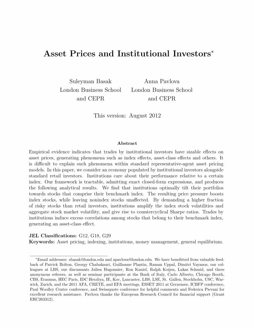
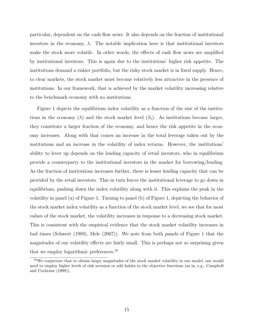
Figure 1 depicts the equilibrium index volatility as a function of the size of the institu-

tions in the economy (λ) and the stock market level (St). As institutions become larger,

they constitute a larger fraction of the economy, and hence the risk appetite in the econ-

omy increases. Along with that comes an increase in the total leverage taken out by the

institutions and an increase in the volatility of index returns. However, the institutions’

ability to lever up depends on the lending capacity of retail investors, who in equilibrium

provide a counterparty to the institutional investors in the market for borrowing/lending.

As the fraction of institutions increases further, there is lesser lending capacity that can be

provided by the retail investors. This in turn forces the institutional leverage to go down in

equilibrium, pushing down the index volatility along with it. This explains the peak in the

volatility in panel (a) of Figure 1. Turning to panel (b) of Figure 1, depicting the behavior of

the stock market index volatility as a function of the stock market level, we see that for most

values of the stock market, the volatility increases in response to a decreasing stock market.

This is consistent with the empirical evidence that the stock market volatility increases in

bad times (Schwert (1989), Mele (2007)). We note from both panels of Figure 1 that the

magnitudes of our volatility effects are fairly small. This is perhaps not so surprising given

that we employ logarithmic preferences.10

10We conjecture that to obtain larger magnitudes of the stock market volatility in our model, one wouldneed to employ higher levels of risk aversion or add habits to the objective functions (as in, e.g., Campbelland Cochrane (1999)).

15

0.2 0.4 0.6 0.8 1

0.151

0.152

0.153

σSt

λ

σSt

20 40 60 80 100

0.151

0.152

0.153

σSt

St

σSt

(a) Effect of the size of institutions (b) Effect of the stock market level

Figure 1: Equilibrium index volatility. This figure plots the index volatility in thepresence of institutions against the fraction of institutions in the economy λ and against thestock market index level St. The dotted lines correspond to the equilibrium index volatilityin the benchmark economy with no institutions. The plots are typical. The parameter valuesare: b = 1, D0 = 1, σ = 0.15, t = 1, T = 5. In panel (a) Dt = 2, and in panel (b) λ = 0.2.

3.2. Risk Taking, Leverage, and Wealth Effects

To further understand the underlying economic mechanisms operating in our model, we look

more closely at the investors’ portfolios in equilibrium. Towards that, we also look at the

investors’ portfolios in terms of the number of shares in the risky stock, i.e.,

πIt = ϕIt

WIt

St

, πRt = ϕRt

WRt

St

,

where as before ϕit denotes the fraction of investor’s wealth invested in the index. This is

to enable us to explicitly identify the nature of the wealth effects in the economy, i.e., who

buys or sells in response to cash flow news. Proposition 3 reports the investors’ equilibrium

portfolios, as well as an important property of the institutional portfolio holdings.

Proposition 3. The institutional and retail investors’ portfolios in equilibrium are given by

πIt = λ1 + bDt

1 + (1− λ) bD0 + λ bDt

(1− λ bDt

1 + (1− λ) bD0 + λ bDt

σ

σSt

+bDt

1 + bDt

σ

σSt

), (11)

πRt = (1− λ)1 + bD0

1 + (1− λ) bD0 + λ bDt

(1− λ bDt

1 + (1− λ) bD0 + λ bDt

σ

σSt

), (12)

16

where σSt is as in Proposition 2.

Consequently, for λ ∈ (0, 1) the institutional investor is always levered, WIt(1− ϕIt) < 0.

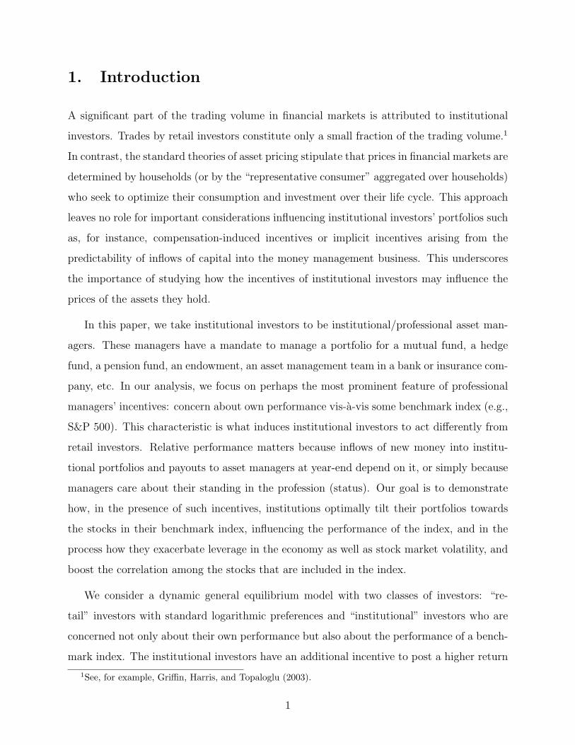
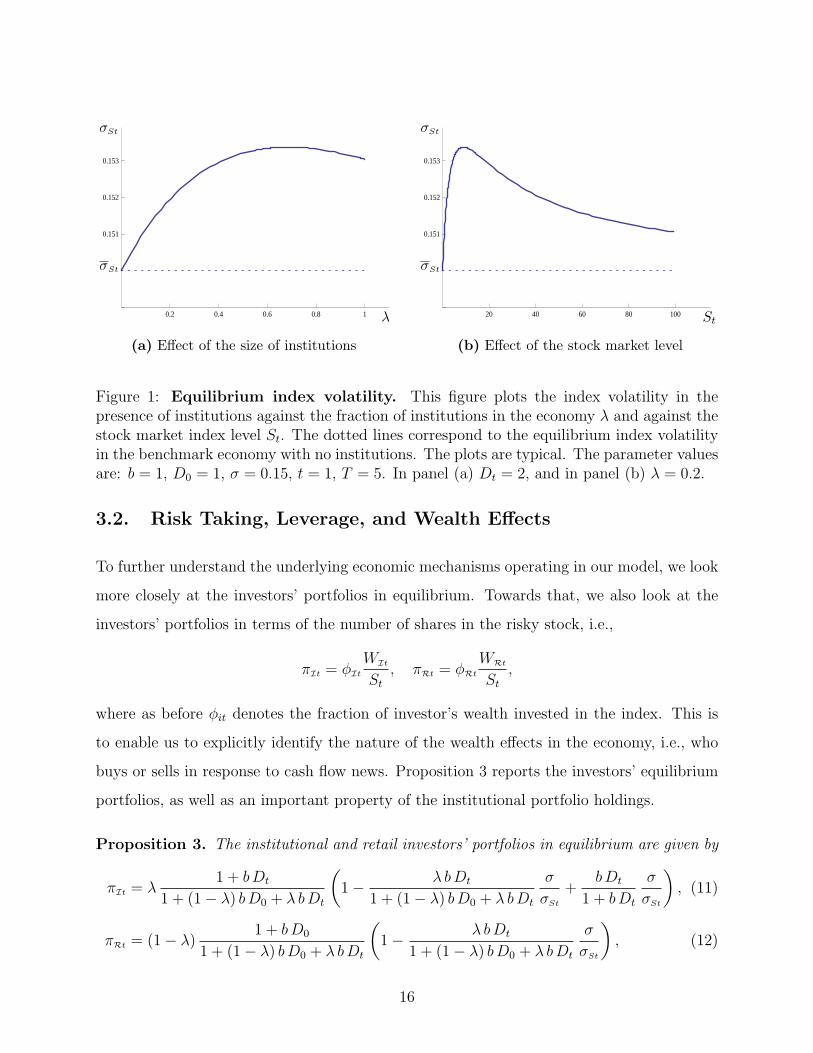
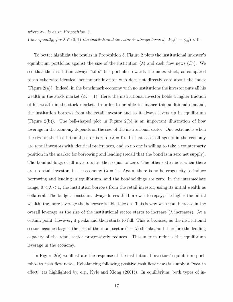
To better highlight the results in Proposition 3, Figure 2 plots the institutional investor’s

equilibrium portfolios against the size of the institution (λ) and cash flow news (Dt). We

see that the institution always “tilts” her portfolio towards the index stock, as compared

to an otherwise identical benchmark investor who does not directly care about the index

(Figure 2(a)). Indeed, in the benchmark economy with no institutions the investor puts all his

wealth in the stock market (ϕI = 1). Here, the institutional investor holds a higher fraction

of his wealth in the stock market. In order to be able to finance this additional demand,

the institution borrows from the retail investor and so it always levers up in equilibrium

(Figure 2(b)). The bell-shaped plot in Figure 2(b) is an important illustration of how

leverage in the economy depends on the size of the institutional sector. One extreme is when

the size of the institutional sector is zero (λ = 0). In that case, all agents in the economy

are retail investors with identical preferences, and so no one is willing to take a counterparty

position in the market for borrowing and lending (recall that the bond is in zero net supply).

The bondholdings of all investors are then equal to zero. The other extreme is when there

are no retail investors in the economy (λ = 1). Again, there is no heterogeneity to induce

borrowing and lending in equilibrium, and the bondholdings are zero. In the intermediate

range, 0 < λ < 1, the institution borrows from the retail investor, using its initial wealth as

collateral. The budget constraint always forces the borrower to repay; the higher the initial

wealth, the more leverage the borrower is able take on. This is why we see an increase in the

overall leverage as the size of the institutional sector starts to increase (λ increases). At a

certain point, however, it peaks and then starts to fall. This is because, as the institutional

sector becomes larger, the size of the retail sector (1− λ) shrinks, and therefore the lending

capacity of the retail sector progressively reduces. This in turn reduces the equilibrium

leverage in the economy.

In Figure 2(c) we illustrate the response of the institutional investors’ equilibrium port-

folios to cash flow news. Rebalancing following positive cash flow news is simply a “wealth

effect” (as highlighted by, e.g., Kyle and Xiong (2001)). In equilibrium, both types of in-

17

0.2 0.4 0.6 0.8 1

0.8

1

1.2

1.4

1.6

ϕI

λ

ϕI

0.2 0.4 0.6 0.8 1

-0.1

-0.2

-0.3

λWI(1− ϕI)

(a) Effect of size of institution (b) Effect of size of institution

0 5 10 15 20

0.1

0.4

0.6

0.8

1

πI

Dt

πI

(c) Effect of cash flow news

Figure 2: The institutional investor’s portfolio holdings. Panels (a) and (b) of thisfigure plot the institution’s fraction of wealth invested in the index ϕI and the bond holdingsWI(1 − ϕI) against the size of the institution λ. Panel (c) plots the institution’s holdingsof the shares of the index πI against cash flow news Dt. The lines for π correspond to theholdings of an otherwise identical investor in the benchmark economy. The plots are typical.In panels (a) and (b) Dt = 2, and in panel (c) λ = 0.2. The remaining parameter values areas in Figure 1.

18

vestors have positive holdings of the risky stock, and so good cash flow news translates into

higher wealth for each investor. As the investors become wealthier, they want to increase

the riskiness of their portfolios, which in this model implies buying more shares of the risky

stock. Of course, for the stock market to clear, both investors cannot be buying the stock

simultaneously; one of them has to sell. To determine who is buying and who is selling, one

can look at the change in the wealth distribution in the economy. In this case, as positive

cash flow news arrives (Dt increases), the wealth distribution shifts in favor of the institu-

tional investor. Intuitively, this is because the institutional portfolio is over-weighted in the

risky stock relative to that of the retail investor, and so good news about the stock produces

a higher return on the institutional portfolio relative to that of the retail investor.11 Hence,

following good cash flow news, the institution buys from the retail investor (Figure 2(c)).

This wealth effect is an important part of the economic mechanisms that operate in our

model. It is useful to stress at this point that the bulk of the related literature, developed

in the framework in which investors have CARA preferences, is not able to capture wealth

effects. The assumption of CARA utilities is made, of course, for tractability. In our model,

tractability is achieved through alternative channels, which we highlight in this section and

the next.

3.3. Sharpe Ratio and Further Discussion

We now explore the behavior of the Sharpe ratio (or market price of risk), stock mean return

per unit volatility κt ≡ µSt/σSt, in the presence of institutions in equilibrium. It has been

well-documented in the data that this quantity is countercyclical. It is of interest to explore

the nature of the time variation in the Sharpe ratios that the presence of institutions may

induce.

11We show formally that the institution becomes wealthier relative to the retail investor following goodcash flow news, i.e., WIt/WRt increases with Dt, in the proof of Proposition 3 in Appendix A. In particular,we show that the wealth distribution is given by

WIt

WRt

=λ

1− λ

1 + bDt

1 + bD0.

19

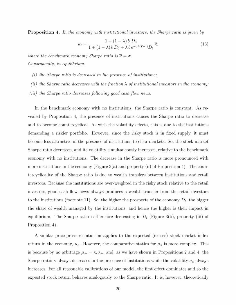
Proposition 4. In the economy with institutional investors, the Sharpe ratio is given by

κt =1 + (1− λ) b D0

1 + (1− λ) bD0 + λ b e−σ2(T−t)Dt

κ, (13)

where the benchmark economy Sharpe ratio is κ = σ.

Consequently, in equilibrium:

(i) the Sharpe ratio is decreased in the presence of institutions;

(ii) the Sharpe ratio decreases with the fraction λ of institutional investors in the economy;

(iii) the Sharpe ratio decreases following good cash flow news.

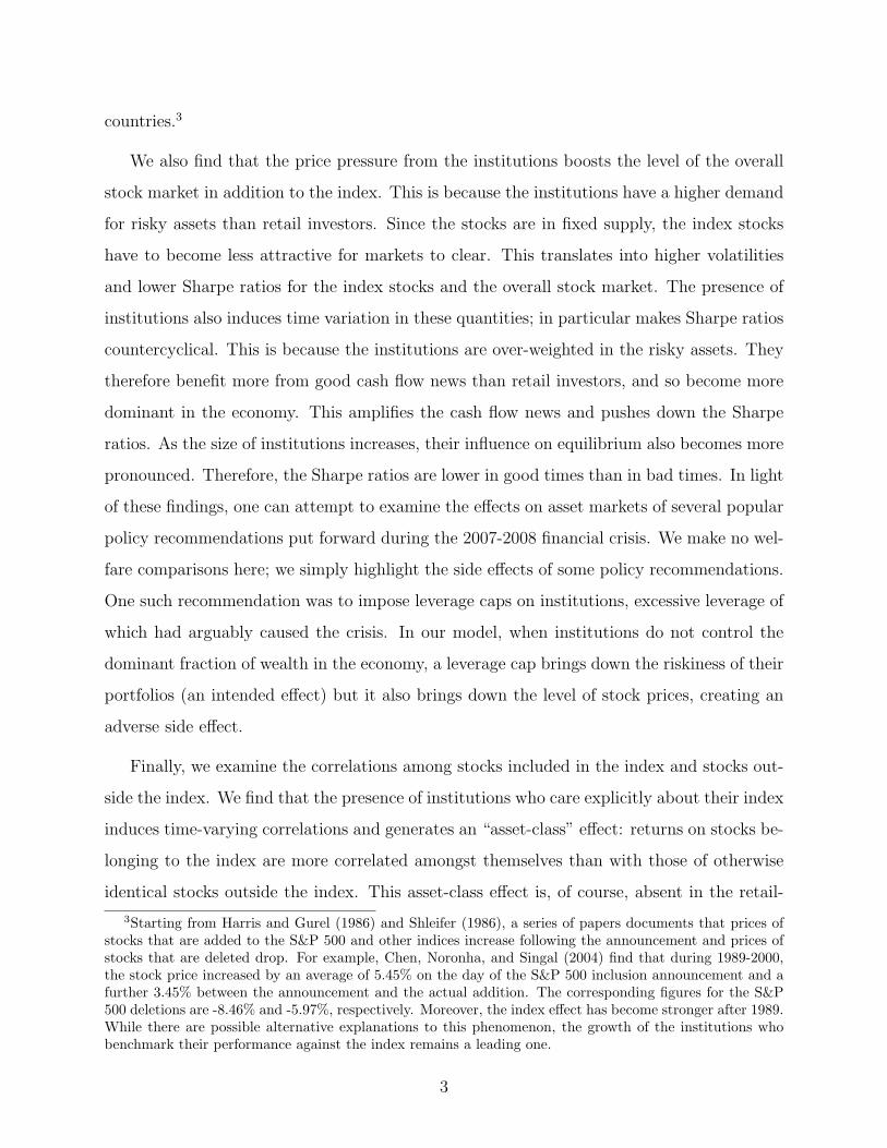
In the benchmark economy with no institutions, the Sharpe ratio is constant. As re-

vealed by Proposition 4, the presence of institutions causes the Sharpe ratio to decrease

and to become countercyclical. As with the volatility effects, this is due to the institutions

demanding a riskier portfolio. However, since the risky stock is in fixed supply, it must

become less attractive in the presence of institutions to clear markets. So, the stock market

Sharpe ratio decreases, and its volatility simultaneously increases, relative to the benchmark

economy with no institutions. The decrease in the Sharpe ratio is more pronounced with

more institutions in the economy (Figure 3(a) and property (ii) of Proposition 4). The coun-

tercyclicality of the Sharpe ratio is due to wealth transfers between institutions and retail

investors. Because the institutions are over-weighted in the risky stock relative to the retail

investors, good cash flow news always produces a wealth transfer from the retail investors

to the institutions (footnote 11). So, the higher the prospects of the economy Dt, the bigger

the share of wealth managed by the institutions, and hence the higher is their impact in

equilibrium. The Sharpe ratio is therefore decreasing in Dt (Figure 3(b), property (iii) of

Proposition 4).

A similar price-pressure intuition applies to the expected (excess) stock market index

return in the economy, µS. However, the comparative statics for µS is more complex. This

is because by no arbitrage µSt = κtσSt, and, as we have shown in Propositions 2 and 4, the

Sharpe ratio κ always decreases in the presence of institutions while the volatility σS always

increases. For all reasonable calibrations of our model, the first effect dominates and so the

expected stock return behaves analogously to the Sharpe ratio. It is, however, theoretically

20

0 0.2 0.4 0.6 0.8 1

0.04

0.07

0.1

0.13

κ

λ

κ

0 2 4 6 8 10

0.07

0.1

0.13

κ

Dt

κ

(a) Effect of the size of institutions (b) Effect of cash flow news

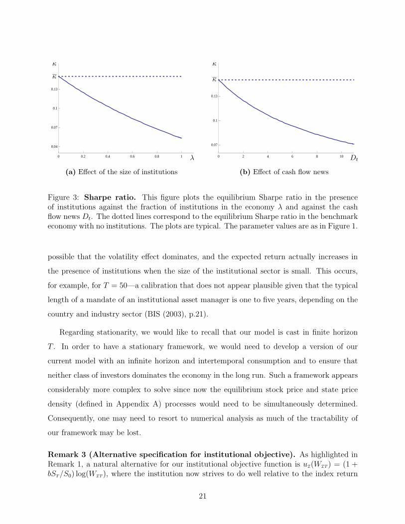
Figure 3: Sharpe ratio. This figure plots the equilibrium Sharpe ratio in the presenceof institutions against the fraction of institutions in the economy λ and against the cashflow news Dt. The dotted lines correspond to the equilibrium Sharpe ratio in the benchmarkeconomy with no institutions. The plots are typical. The parameter values are as in Figure 1.

possible that the volatility effect dominates, and the expected return actually increases in

the presence of institutions when the size of the institutional sector is small. This occurs,

for example, for T = 50—a calibration that does not appear plausible given that the typical

length of a mandate of an institutional asset manager is one to five years, depending on the

country and industry sector (BIS (2003), p.21).

Regarding stationarity, we would like to recall that our model is cast in finite horizon

T . In order to have a stationary framework, we would need to develop a version of our

current model with an infinite horizon and intertemporal consumption and to ensure that

neither class of investors dominates the economy in the long run. Such a framework appears

considerably more complex to solve since now the equilibrium stock price and state price

density (defined in Appendix A) processes would need to be simultaneously determined.

Consequently, one may need to resort to numerical analysis as much of the tractability of

our framework may be lost.

Remark 3 (Alternative specification for institutional objective). As highlighted inRemark 1, a natural alternative for our institutional objective function is uI(WIT ) = (1 +bST/S0) log(WIT ), where the institution now strives to do well relative to the index return

21

ST/S0. Following the analysis of Section 2.2 and Appendix A, for this objective function, wederive the institutional investor’s optimal portfolio to be

ϕIt =µSt

σ2St

+bDt/S0

1 + bDt/S0

σ

σSt

.

We again obtain the tilt in the institutional portfolio towards the index, arising due to theinstitution’s desire to perform well as compared to the index return. Moving to equilibrium,similarly to Section 3.1, we determine the equilibrium market index level as

St = St1 + bD0/S0 + λ b(Dt/S0 −D0/S0)

1 + bD0/S0 + λ b (e−σ2(T−t)Dt/S0 −D0/S0), (14)

where St is the equilibrium index level in the benchmark economy as in (9). The endogenousinitial index level S0 solves (14), and it can be shown that the unique strictly positive solutionis given by

S0 = D0

√B2 − 4b e−σ2T −B

2,

where B = b−e−σ2T+λb(be−σ2T−1). Comparing with Proposition 1 of the earlier analysis, wesee that under this alternative specification, we have a very similar index level expression.The main difference is that the index cash flow news news quantity D is now expressedper unit of the initial index level. More importantly, the price pressure from the institutionsincreases the stock index level, as before. Similarly, all other results and intuitions, includingthe index volatility, Sharpe ratio, go through for this alternative specification, with similarlymodified expressions.

3.4. Asset Pricing Implications of Popular Policy Measures

The two main policy measures we would like to consider in the context of our model are the

effects of deleveraging (a mandate to reduce leverage) and the effects of a transfer of capital

to leveraged institutions. These two policy instruments have widely been employed during

the 2007-2008 financial crisis. The objective, of course, was to improve the balance sheets

of individual institutions in difficulty. But these policy actions, given their size and scope,

inevitably had an effect on the overall economy, including asset prices. In this paper, we

have nothing to say about the welfare consequences of these policies; in future research it

would be interesting to address this question. Our goal here is to simply analyze the spillover

effects of the popular policy measures on asset prices in our model.

At this point, we also draw a distinction between long-only institutions (“real money”)

and leveraged institutions (“leveraged money”). So far we have only dealt with the latter

22

category. We model long-only institutions, L, in a very simple form: these institutions do not

solve any optimization problem but simply buy and hold the risky stock they are endowed

with. The initial endowments of the retail investors, leveraged institutions, and long-only

institutions are nowWR0 = (1−λ)S0, WI0 = λθS0, andWL0 = λ(1−θ)S0, respectively. That

is, the endowment of the retail investors is as before, but the endowment of institutions is

now divided between the leveraged institutions and long-only institutions in proportions θ

and 1− θ, respectively. The new parameter θ ∈ (0, 1) then captures the mass of “leveraged

money” as a fraction of funds held (initially) by institutions. By reducing θ we can model a

transfer of assets from leveraged institutions to long-only, or deleveraging.

Denote by λ′ the endowment held by the leveraged institutional investors relative to the

combined endowment of all active investors (the retail and leveraged institutional investors),

so thatλ′

1− λ′=

λθ

1− λ.

Proposition 5 summarizes how asset prices and equilibrium portfolios in our model are af-

fected by the introduction of this new class of institutions.

Proposition 5. The equilibrium index level, volatility, and institutional portfolio in thepresence of long-only and leveraged institutions are given by their counterparts in Propo-sitions 1–3, but with λ replaced by λ′.

Consequently, the equilibrium stock price and volatility are higher in the presence of in-stitutions and the stock price increases further as the fraction of leveraged institutions, θ,increases.

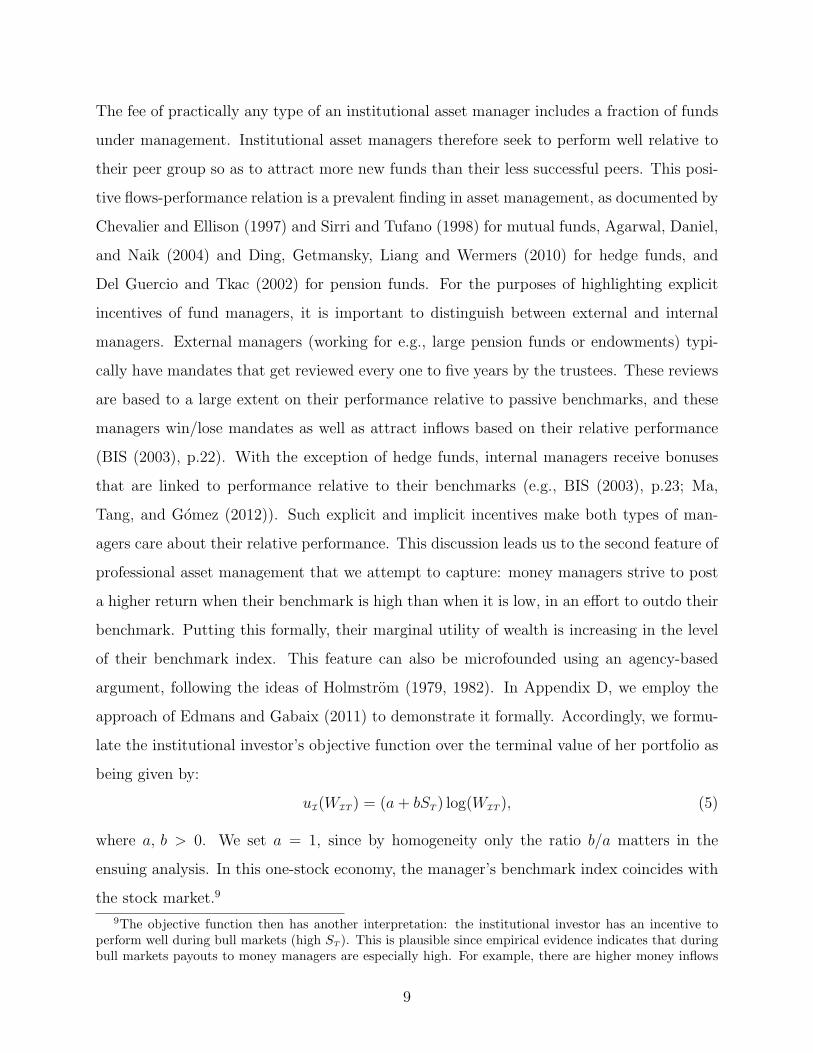
We again find it useful to highlight the results of the proposition in a figure. Figure 4

plots the bond and stock holdings of the leveraged institution, as well as the equilibrium

stock market index and its volatility, as functions of the size of the “leveraged money” sector

θ. The figure confirms that the stock price and the stock holdings of the leveraged institution

are unambiguously increasing in θ. The effect of θ on bondholdings (leverage), however, is

not necessarily unambiguous. It depends on the total size of the institutional investors (both

real and leveraged money) relative to that of the retail investors. If there is enough lending

capacity in the economy—the mass of retail investors is high—then the total amount of

borrowing always increases with the size of the leveraged money sector. If, however, the

23

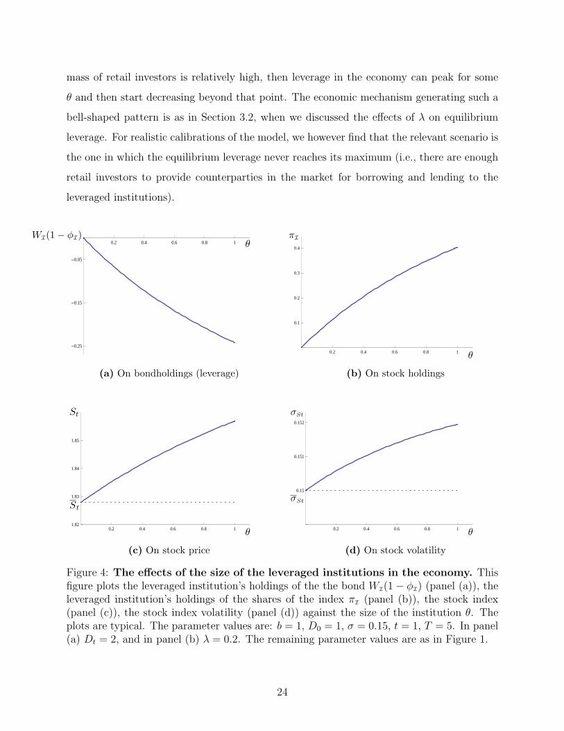
mass of retail investors is relatively high, then leverage in the economy can peak for some

θ and then start decreasing beyond that point. The economic mechanism generating such a

bell-shaped pattern is as in Section 3.2, when we discussed the effects of λ on equilibrium

leverage. For realistic calibrations of the model, we however find that the relevant scenario is

the one in which the equilibrium leverage never reaches its maximum (i.e., there are enough

retail investors to provide counterparties in the market for borrowing and lending to the

leveraged institutions).

0.2 0.4 0.6 0.8 1

-0.05

-0.15

-0.25

θWI(1− ϕI)

0.2 0.4 0.6 0.8 1

0.1

0.2

0.3

0.4

πI

θ

(a) On bondholdings (leverage) (b) On stock holdings

0.2 0.4 0.6 0.8 11.82

1.83

1.84

1.85

St

θ

St

0.2 0.4 0.6 0.8 1

0.15

0.151

0.152

σSt

θ

σSt

(c) On stock price (d) On stock volatility

Figure 4: The effects of the size of the leveraged institutions in the economy. Thisfigure plots the leveraged institution’s holdings of the the bond WI(1− ϕI) (panel (a)), theleveraged institution’s holdings of the shares of the index πI (panel (b)), the stock index(panel (c)), the stock index volatility (panel (d)) against the size of the institution θ. Theplots are typical. The parameter values are: b = 1, D0 = 1, σ = 0.15, t = 1, T = 5. In panel(a) Dt = 2, and in panel (b) λ = 0.2. The remaining parameter values are as in Figure 1.

24

a. Effects of deleveraging

In our framework, we model deleveraging as a transfer of assets from leveraged institutions

to long-only institutions at time 0. This policy can be interpreted as a requirement that a

fraction of leveraged institutions must convert into “real money” long-only investors. In our

model, we capture this as a reduction in the fraction of leveraged institutions θ.

Figure 4(a) reveals that a reduction in the mass of leveraged institutions indeed decreases

the total leverage in the economy, with the total amount of outstanding bondholdings going

down. Not being able to finance a risky asset position of the same size as prior to deleveraging,

the institutional sector reduces its demand for the risky stock and the stock holdings of the

sector fall (Figure 4(b)). While the deleveraging policy does achieve its desired outcome—the

riskiness of the institutional portfolios going down—it does, however, come with side effects.

The most notable one is that a reduction in the number of leveraged institutions also brings

down the stock market index (Figure 4(c)). This effect is a simply a consequence of the drop

in demand for the stock index by the institutions.

b. Effects of a capital injection

In our model, a capital injection into leveraged institutions at time 0 is equivalent to

an increase in the mass of leveraged institutions θ. So the effects of such an injection are

the opposite from those of deleveraging. This policy does boost the stock market index

(Figure 4(c)) because a capital injection increases the demand of the institutions for the

risky stock and they purchase more shares of it (Figure 4(b)). As a result of the stock

price increase, everybody in the economy, including retail investors, becomes wealthier. But

along with the run-up in the stock market, comes an increase in the leverage of institutional

investors (Figure 4(a)). When the institutions do not control a dominant fraction of the

financial wealth in the economy (θ ≪ 1), the stock price volatility also increases (Figure 4(d)).

These side effects could be undesirable.

25

4. Multiple Stocks, Asset Classes, and Correlations

Our analysis has so far been presented in the context of a single-stock economy. Our goal

in this section is to demonstrate how our results generalize in a multi-stock economy and to

examine the correlations between stock returns. For the latter, we aim to demonstrate how

institutional investors in our model generate an “asset-class” effect—i.e., how they make

returns of assets belonging to an index to be more correlated amongst themselves than with

those of otherwise identical assets outside the index.

4.1. Economic Setup

The general version of our economy features N risky stocks and N sources of risk, generated

by a standard N -dimensional Brownian motion ω = (ω1, . . . , ωN)⊤, as well as a riskless

bond.12 Each stock price, Sj, j = 1, . . . , N , is posited to have dynamics

dSjt = Sjt[µSjtdt+ σSjt

dωt], (15)

where the vector of stock mean returns µS ≡ (µS1, . . . , µSN

)⊤ and the stock volatility matrix

σS ≡ {σSjℓ, j, ℓ = 1, . . . , N} are to be determined in equilibrium. The (instantaneous)

correlation between stock j and ℓ returns, ρjℓt ≡ σ⊤SjtσSℓt/

√||σSjt||2||σSℓt

||2, is also to be

endogenously determined.13 The value of the equity market portfolio, SMKT , is the sum of

the risky stock prices:

SMKT t =N∑j=1

Sjt, (16)

with posited dynamics

dSMKT t = SMKT t[µMKT t dt+ σMKT t dωt]. (17)

12We include the bond to keep the discipline of a standard asset pricing framework, which serves as ourbenchmark. However, our analysis is equally valid without the bond present and the investment opportunitiesrepresented only by risky stocks. Such a variant of our model is perhaps more appropriate for modeling funds,whose investments are typically restricted to a single asset class, e.g., equities. We present the analysis forthe stocks-only economy in Appendix C.

13The notation ||z|| denotes the dot product z · z.

26

Additionally, there is a value-weighted index (in terms of returns) made up of the first M

stocks in the economy:

SIt =M∑i=1

Sjt.

This stock index SI represents a specific asset class in the economy, and we will refer to the

first M stocks as “index stocks” and the remainder N −M stocks as the nonindex stocks.

Each stock is in positive net supply of one share. Its terminal payoff (or dividend) DjT ,

due at time T , is determined by the process

dDjt = Djtσjdωt, (18)

where σj > 0 is constant for all stocks except for the last ones in the index and the market (the

M th and N th stocks).14 The process Djt represents the cash flow news about the terminal

stock dividendDjT , and SjT = DjT . For expositional clarity and the thought experiment that

we are going to undertake in this section, assume that the stocks’ fundamentals (dividends)

are independent. We thus assume that only the jth element of σj in (18) is nonzero, while

all other elements are zero, so that the volatility matrix of cash flow news is diagonal. This

implies zero correlation among all stocks’ cash flow news, σ⊤j σℓ = 0 for all j = ℓ.

The stock market has a terminal payoff SMKT T = DT , given by the terminal value of the

process

dDt = Dtσdωt, (19)

where σ > 0 is constant. Similarly, the index has a terminal value SIT = IT , determined by

the process

dIt = ItσIdωt, (20)

with σI > 0 constant and having its first M components non-zero and the remainder N −M

components zero. The latter assumption is to make σI consistent with our assumptions

14That is, we do not explicitly specify the process of the cash flow news for the last stock in the index andin the market; but, in what follows, we specify processes for the sums of all stocks in the index and in themarket. This modeling device is inspired by Menzly, Santos, and Veronesi (2004). It allows us to assumethat the stock market and the index cash flow news follow geometric Brownian motion processes (equations(19) and (20)), which improves the tractability of the model considerably. In related analysis, we find thatone may alternatively not assume a geometric Brownian motion process for the index cash flow news, butinstead assume that stock M ’s dividend follows a geometric Brownian motion process. In that case, theanalogs of the expressions that we report below are less elegant, and several results can be obtained onlynumerically.

27

about the individual stocks’ cash flow news processes. Accordingly, while the index stocks’

cash flow news have positive correlation with that of the index, σ⊤j σI > 0, j = 1, . . . ,M , the

cash flow news of the nonindex stocks have zero correlation, σ⊤k σI = 0, k =M + 1, . . . , N .

Each type of investor i = I, R now dynamically chooses a multi-dimensional portfolio

process ϕi, where ϕi = (ϕi1, . . . , ϕiN)⊤ denotes the portfolio weights in each risky stock. The

portfolio value Wi then has the dynamics

dWit = Witϕ⊤it [µStdt+ σStdωt]. (21)

The retail investor is initially endowed with 1 − λ fraction of the stock market, providing

initial assets WR0 = (1−λ)SMKT0, and has the same objective function as in the single-stock

case: uR(WRT ) = log(WRT ). The institutional investor is initially endowed with λ fraction

of the stock market and hence has initial assets worth WI0 = λSMKT0. In this multi-stock

version of our economy, the objective function of the institution is given by

uI(WIT ) = (1 + bIT ) log(WIT ), (22)

where b > 0 and IT = SIT is the terminal value of the index (composed of the first M stocks

in the economy). Here, the institutional investor has a benchmark that is distinct from the

overall stock market. He now strives to perform particularly well when a specific asset class,

represented by the index SI, does well. One can think of this asset class as value stocks,

technology stocks, or the stocks included in the S&P 500 index.

4.2. Investors’ Portfolio Choice

We are now ready to examine how the results derived in the earlier analysis extend to the

multi-stock case. We start with Lemma 2, which reports the investors’ optimal portfolios in

closed form.

Lemma 2. The institutional and retail investors’ optimal portfolio processes are given by

ϕIt = (σStσ⊤St)

−1µSt +b It

1 + b It(σ⊤

St)−1σI, (23)

ϕRt = (σStσ⊤St)

−1µSt. (24)

Moreover,

28

(i) The institutional investor’s hedging portfolio, the second term in (23), has positiveportfolio weights in the index stocks j = 1, . . . , N − 1, but zero weights in the nonindexstocks in equilibrium;

(ii) The institutional investor invests a higher fraction of wealth in the index stocks j =1, . . . , N − 1 than the retail investor, while holding the same fractions in the nonindexstocks as the retail investor.

The investors’ portfolios in (23)–(24) are natural multi-stock generalizations of the single-

stock case. Again, the institutional investor holds the mean-variance efficient portfolio plus

an additional portfolio hedging her against fluctuations in her index. In our single-stock

economy, the hedging demand of the institutional investor generates a tilt in her portfolio

towards the risky stock, as compared to the retail investor. The multi-stock economy refines

this implication. It is not the case that the institutional investor simply desires to take on

more risk; rather, she demands a portfolio that is highly correlated with her index. This is

why she has the same demand for the nonindex stocks as the retail investor, but demands

additional holdings of index stocks, so as to not fall behind when the index does well. As

we will see shortly, this excess demand for index stocks by the institution is the key driver

of the index effect in our model.

From Lemma 2, we also see that the institution’s optimal portfolio satisfies a three-fund

separation property, with the three funds being the mean-variance efficient portfolio, the

intertemporal hedging portfolio, and the riskless bond. The importance of this decomposition

will become apparent later, when we discuss the asset-class effect in Section 4.4. For now,

we just note that the hedging portfolio has positive portfolio weights in the index stocks,

and when the institution gets wealthier—following for example, good cash flow news—she

demands more shares of the index stocks (a wealth effect). This additional price pressure

(beyond the standard increase in demand for the mean-variance portfolio) is applied to all

index stocks simultaneously. There is no additional demand for the nonindex stocks.

Our implications for the higher risk-taking by institutions, who take on leverage in order

to finance the hedging portfolio, remain the same as in our earlier analysis. We do not repeat

them here and proceed to exploring the additional insights that a multiple stock environment

is able to offer.

29

4.3. Stock Prices and Index Effect

Proposition 6 reports the equilibrium stock prices in closed form and highlights the effects

of institutions on stock prices.

Proposition 6. In the economy with institutional investors and multiple risky stocks, theequilibrium prices of the market portfolio, index stocks j = 1, . . . ,M −1 and nonindex stocksk =M + 1, . . . , N − 1 are given by

SMKT t = SMKT t1 + b I0 + λ b (It − I0)

1 + b I0 + λ b (e−σ⊤I σ(T−t)It − I0)

, (25)

Sjt = Sjt1 + b I0 + λ b (e(−σ⊤

I σ+σ⊤j σI)(T−t)It − I0)

1 + b I0 + λ b (e−σ⊤I σ(T−t)It − I0)

, (26)

Skt = Skt, (27)

where SMKT t, Sjt, and Skt are the equilibrium prices of the market portfolio, index andnonindex stocks, respectively, in the benchmark economy with no institutions, given by

SMKT t = e−||σ||2(T−t)Dt, Sjt = e−σ⊤j σ(T−t)Djt, Skt = e−σ⊤

k σ(T−t)Dkt. (28)

Consequently, the market portfolio and index stock prices are increased in the presence ofinstitutional investors, while nonindex stock prices are unaffected.

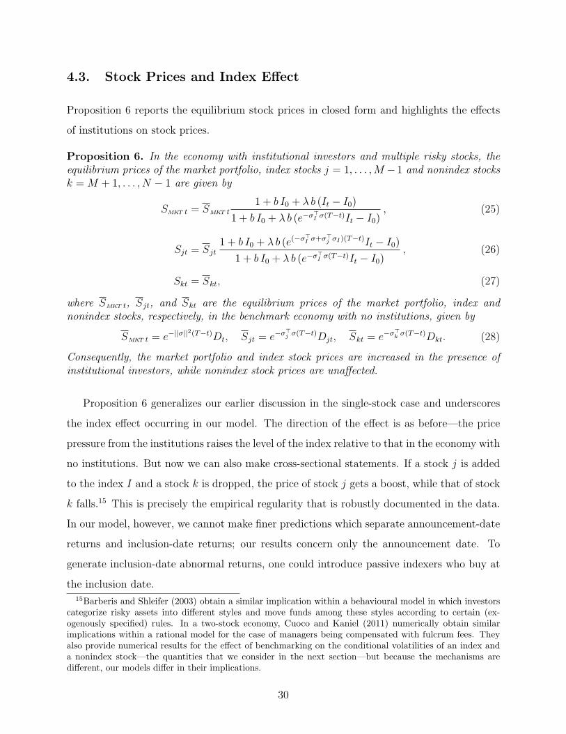
Proposition 6 generalizes our earlier discussion in the single-stock case and underscores

the index effect occurring in our model. The direction of the effect is as before—the price

pressure from the institutions raises the level of the index relative to that in the economy with

no institutions. But now we can also make cross-sectional statements. If a stock j is added

to the index I and a stock k is dropped, the price of stock j gets a boost, while that of stock

k falls.15 This is precisely the empirical regularity that is robustly documented in the data.

In our model, however, we cannot make finer predictions which separate announcement-date

returns and inclusion-date returns; our results concern only the announcement date. To

generate inclusion-date abnormal returns, one could introduce passive indexers who buy at

the inclusion date.15Barberis and Shleifer (2003) obtain a similar implication within a behavioural model in which investors

categorize risky assets into different styles and move funds among these styles according to certain (ex-ogenously specified) rules. In a two-stock economy, Cuoco and Kaniel (2011) numerically obtain similarimplications within a rational model for the case of managers being compensated with fulcrum fees. Theyalso provide numerical results for the effect of benchmarking on the conditional volatilities of an index anda nonindex stock—the quantities that we consider in the next section—but because the mechanisms aredifferent, our models differ in their implications.

30

0.2 0.4 0.6 0.8 1

4.8

4.85

4.9

4.95

Sjt, Skt

λ

Skt

Figure 5: An index effect. This figure plots the prices of an index stock Sj (solid line)and a nonindex stock Sk (dotted line) in the presence of institutions against the fraction ofinstitutions in the economy λ. The plot is typical. The parameter values are: M = 3, N = 6,j = 1, k = 4, σj = 0.15 ij, where ij is an N-dimensional unit vector with the jth element

equal to 1 and the remaining elements equal to 0, σk = 0.15 ik, σI = 0.15∑M

j=1 ij/√M ,

σ = 0.15×1/√N , where 1 is an N-dimensional vector of ones, I0 = 1, It = 2, and Dt = 5.

The normalizations by√M and

√N are adopted so as to keep ||σI|| and ||σ|| constant as

we vary the number of stocks. The remaining parameters are as in Figure 1.

Figure 5 presents a plot of the price of an index stock relative to that of an otherwise

identical nonindex stock. The plot is drawn as a function of the size of institutions λ. As

expected, we see that the stock price is increasing with λ. This is due to the additional price

pressure on index stocks as the institutional sector becomes larger. We also observe that the

magnitudes are reasonable for our calibration. Chen, Noronha, and Singal (2004) find that

during 1989-2000, a stock’s price increases by an average of 5.45% on the day of the S&P

500 inclusion announcement and a further 3.45% between the announcement and the actual

addition. The effects that we find are smaller, but roughly in line with these figures.

4.4. Stock Volatilities, Correlations, and Asset-class Effects

We now turn to examining the implications of our model for stock return volatilities and

correlations. We report them in the following proposition in closed form.

Proposition 7. In the economy with institutional investors and multiple risky stocks, theequilibrium volatilities of the market portfolio, index stocks j = 1, . . . ,M − 1, and nonindex

31

stocks k =M + 1, . . . , N − 1 are given by

σMKT t = σMKT t + λ b σI

(1− e−σ⊤σI(T−t)

)(1 + (1− λ) b I0)It(

1 + (1− λ) b I0 + λ b e−σ⊤I σ(T−t)It

)(1 + (1− λ) b I0 + λ b It)

, (29)

σSjt = σSjt + λ b σI

×

(1− e−σ⊤

j σI(T−t))(1 + (1− λ) b I0)e

(−σ⊤I σ+σ⊤

j σI)(T−t)It(1 + (1− λ) b I0 + λ b e−σ⊤

I σ(T−t)It

)(1 + (1− λ) b I0 + λ b e(−σ⊤

I σ+σ⊤j σI)(T−t)It

) ,(30)

σSkt = σSkt, (31)

where σMKT t, σSjt, and σSkt are the equilibrium market portfolio, index stock, and nonindexstock volatilities, respectively, in the benchmark economy with no institutions, given by

σMKT t = σ, σSjt = σj, σSkt = σk. (32)

Consequently, in equilibrium:

(i) The market portfolio and index stock volatilities are increased in the presence of insti-tutional investors, while nonindex stock volatilities are unaffected;

(ii) The correlations between index stocks are increased in the presence of institutional in-vestors, while the correlations between nonindex stocks and between index and nonindexstocks are unaffected.

As one could expect from our earlier analysis, only the volatilities of the index stocks

change in the presence of institutions; the volatilities of the nonindex stocks remain un-

changed. The index stocks become riskier for the same reason as in the single-stock economy:

the risk appetite of in the economy is higher in the presence of institutional investors.

The multiple stock formulation offers additional insights, allowing us to explore how the

presence of institutions affects the correlations of stock returns. These results, based on

fully analytical closed-form expressions, are reported in Proposition 7. Consistent with the

empirical evidence on asset-class effects, we find that the presence of institutions increases

the correlations among the stocks included in their index. The intuition is as follows. In the

benchmark retail-investor-only economy, the cash flow news on all stocks are independent,

and the stock returns turn out to be independent as well. Now consider the economy with

32

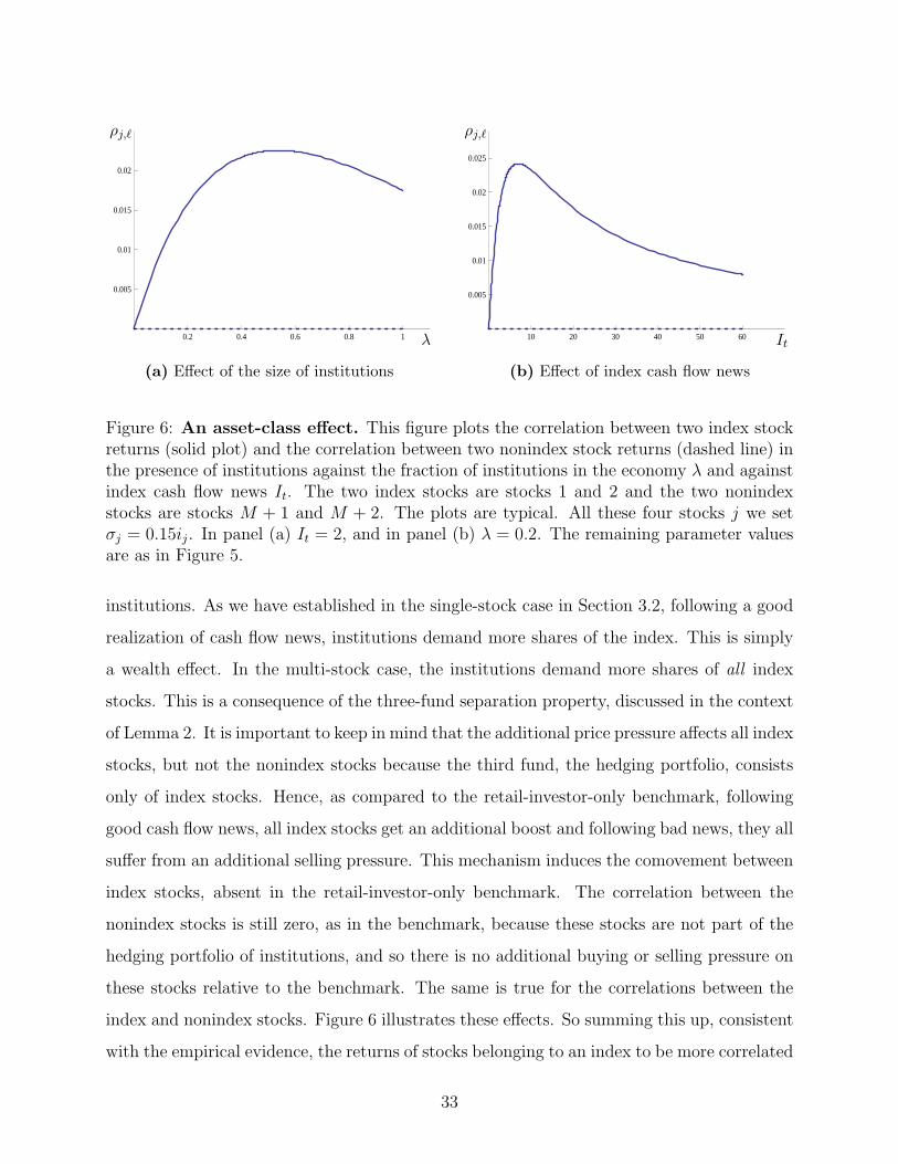
0.2 0.4 0.6 0.8 1

0.005

0.01

0.015

0.02

ρj,ℓ

λ 10 20 30 40 50 60

0.005

0.01

0.015

0.02

0.025

ρj,ℓ

It

(a) Effect of the size of institutions (b) Effect of index cash flow news

Figure 6: An asset-class effect. This figure plots the correlation between two index stockreturns (solid plot) and the correlation between two nonindex stock returns (dashed line) inthe presence of institutions against the fraction of institutions in the economy λ and againstindex cash flow news It. The two index stocks are stocks 1 and 2 and the two nonindexstocks are stocks M + 1 and M + 2. The plots are typical. All these four stocks j we setσj = 0.15ij. In panel (a) It = 2, and in panel (b) λ = 0.2. The remaining parameter valuesare as in Figure 5.

institutions. As we have established in the single-stock case in Section 3.2, following a good

realization of cash flow news, institutions demand more shares of the index. This is simply

a wealth effect. In the multi-stock case, the institutions demand more shares of all index

stocks. This is a consequence of the three-fund separation property, discussed in the context

of Lemma 2. It is important to keep in mind that the additional price pressure affects all index

stocks, but not the nonindex stocks because the third fund, the hedging portfolio, consists

only of index stocks. Hence, as compared to the retail-investor-only benchmark, following

good cash flow news, all index stocks get an additional boost and following bad news, they all

suffer from an additional selling pressure. This mechanism induces the comovement between

index stocks, absent in the retail-investor-only benchmark. The correlation between the

nonindex stocks is still zero, as in the benchmark, because these stocks are not part of the

hedging portfolio of institutions, and so there is no additional buying or selling pressure on

these stocks relative to the benchmark. The same is true for the correlations between the

index and nonindex stocks. Figure 6 illustrates these effects. So summing this up, consistent

with the empirical evidence, the returns of stocks belonging to an index to be more correlated

33

amongst themselves than with those of otherwise identical stocks outside the index.

Figure 6(b) depicts the time-variation in the index stock correlations. The pattern here

is similar to the one observed for the conditional volatilities of the stocks (Figure 1). The

institutions are over-weighted in the index stocks, and therefore good index cash flow news

create a wealth transfer from the retail investors to the institutions. In good states of the

world (high It), the institutions dominate the economy and in bad states (low It) the retail

investors control a larger share of total wealth. The correlations peak when the investor

heterogeneity is the highest. To the right of the peak, the correlations decline, which resemble

their behavior in the data.

5. Summary of Key Predictions and Empirical Impli-

cations

Institutions and the incentives they face feature prominently in models of corporate finance

and banking, but they have largely been ignored in the standard asset pricing theory. In

this paper, we develop an asset-pricing model that incorporates incentives of institutional

investors to do well relative to their index. We demonstrate that this simple ingredient

has profound implications for asset prices. In particular, it generates index effects and

creates excess correlations among stocks belonging to an index (an asset-class effect). It also

increases volatilities of index stocks and the overall market volatility. Moreover, the presence

of institutions decreases the market Sharpe ratio, making it countercyclical.

It is difficult to obtain differential predictions for index and nonindex stocks within

(heterogeneous-agent) consumption-based asset pricing models. For a standard model to

deliver similar results, one would require that either (i) risk aversions “with respect to dif-

ferent stocks” are different, or (ii) capital constraints are more stringent for nonindex stocks

than for index stocks, or (iii) agents have more optimistic beliefs about index stocks than

nonindex stocks. Within a standard asset pricing model, these assumptions appear some-

what contrived, and we believe that benchmarking considerations represent a more plausible

explanation.

34

Empirical literature lends support to all our key predictions. The extensive literature on

index effects growing out of Harris and Gurel (1986) and Shleifer (1986) has now confirmed

in many countries and many markets that stocks rise when added to an index (e.g., Wurgler

and Zhuravskaya (2002), Chen, Noronha, and Singal (2004) and Greenwood (2005)). The

presence of asset-class effects has been documented by e.g., Barberis, Shleifer, and Wurgler

(2005) and Boyer (2011) for stocks, Rigobon (2002) for sovereign bonds, Tan and Xiong

(2011) for commodity futures. There is a large literature documenting that institutional

ownership increases stock volatility (e.g., Bushee and Noe (2000), Sias (2006)). Recently,

Greenwood and Thesmar (2012) linked this finding to the asset-class effect. Gabaix et al.

(2006) argue that institutions amplify volatility by examining trades of very large institu-

tional investors. Our finding that the Sharpe ratio is countercyclical is also well-documented

in the literature (see, e.g., Lettau and Ludvigson (2010)). Our model also predicts that the

Sharpe ratios of index stocks are lower than those of nonindex stocks—this is a testable

implications that future research might explore. Finally, Asparouhova et al. (2010) pro-

vide experimental support in favor of our model by documenting significant effects of money

managers on asset prices in a large-scale experimental setting.

We left for future research several unexplored implications and potential extensions of

our model. The presence of institutions may generate momentum of stock returns. Recently,

the link between institutional fund flows and momentum has been established theoretically

by Vayanos and Woolley (2010) and empirically by Lou (2009). The explanation in Vayanos

and Woolley relies additionally on delayed reaction of traders; it would be interesting to

see whether our model can also generate momentum and whether one needs to assume

further that traders cannot immediately rebalance. Another fruitful avenue to explore is to

endogenize the reward for good performance relative to an index (as in, for example, Berk

and Green (2004)).

35

References

Agarwal, V., Daniel, N.D., and N. Naik, 2004, “Flows, Performance, and Managerial In-centives in Hedge Funds,” working paper, London Business School.

Asparouhova, E., Bossaerts, P., Copic, J., Cornell, B., Cvitanic, J., and D. Meloso, 2010,“Experiments on Asset Pricing under Delegated Portfolio Management,” working pa-per, University of Utah.

Arora, N., N. Ju, and H. Ou-Yang, 2006, “A Model of Asset Pricing under Portfolio Dele-gation and Differential Information,” working paper, University of North Carolina.

Ball, S., Eckel, C., Grossman, P.J., and W. Zame, 2001, “Status in Markets,” QuarterlyJournal of Economics, 116(1), 161-188.

Barberis, N., and A. Shleifer, 2003, “Style Investing,” Journal of Financial Economics,68(2), 161-199.

Barberis, N., A. Shleifer, and J. Wurgler, 2005, “Comovement,” Journal of Financial Eco-nomics, 75, 283-317.

Basak, S., A. Pavlova, and A. Shapiro, 2007, “Optimal Asset Allocation and Risk Shiftingin Money Management,” Review of Financial Studies, 20(5), 1583-1621.

Basak, S., A. Pavlova, and A. Shapiro, 2008, “Offsetting the Implicit Incentives: Benefitsof Benchmarking in Money Management,” Journal of Banking and Finance, 32(9),1883-1893.

Binsbergen, J.H.v., M.W. Brandt, and R.S.J. Koijen, 2008, “Optimal Decentralized Invest-ment Management,” Journal of Finance, 63, 1849-1895.

BIS, 2003, “Incentive structures in Institutional Asset Management and their Implicationsfor Financial Markets,” Committee on the Global Financial System, Bank for Interna-tional Settlements, Basel.

Berk, J., and R. Green, 2004, “Mutual Fund Flows and Performance in Rational Markets,”Journal of Political Economy, 112, 1269-1295.

Boyer, B., 2011, “Style Related Comovement: Fundamentals or Labels?,” Journal of Fi-nance, forthcoming.

Brennan, M. J., 1993, “Agency and Asset Pricing,” working paper, UCLA.

Brennan, M. J., and F. Li, 2008, “Agency and Asset Pricing,” working paper, UCLA.

Bushee, B.J., and C. F. Noe, 2000, “Corporate disclosure practices, institutional investors,and stock return volatility,” Journal of Accounting Research, 38, 171-202.

Campbell J., and J. Cochrane, 1999, “By Force of Habit: A Consumption-Based Explana-tion of Aggregate Stock Market Behavior,” Journal of Political Economy, 107, 205-251.

Chen, H., G. Noronha, and V. Singal, 2004, “The Price Response to S&P 500 Index Ad-ditions and Deletions: Evidence of Asymmetry and a New Explanation,” Journal ofFinance, 59, 1901-29.

Chen, H., and G. Pennacchi, 2009, “Does Prior Performance Affect a Mutual Fund’s Choiceof Risk?,” Journal of Financial and Quantitative Analysis, 44, 745-775.

36

Chevalier, J. and G. Ellison, 1997, “Risk Taking by Mutual Funds as a Response to Incen-tives,” Journal of Political Economy, 105(6), 1167-1200.

Cornell, B., and R. Roll, 2005, “A Delegated-Agent Asset-Pricing Model,” Financial Ana-lysts Journal, 61, 57-69.

Cuoco, D., and R. Kaniel, 2011, “Equilibrium Prices in the Presence of Delegated PortfolioManagement,” Journal of Financial Economics, 101(2), 264-296.

Dasgupta, A., and A. Prat, 2008, “Information Aggregation in Financial Markets withCareer Concerns,” Journal of Economic Theory, 143, 83-113.

Dasgupta, A., A. Prat, and M. Verardo, 2008, “The Price Impact of Institutional Herding,”working paper, London School of Economics.

DeMarzo, P., R. Kaniel, and I. Kremer, 2004, “Diversification as a Public Good: Commu-nity Effects in Portfolio Choice,” Journal of Finance, 59, 1677-1716.

DeMarzo, P., R. Kaniel, and I. Kremer, 2008, “Relative Wealth Concerns and FinancialBubbles,” Review of Financial Studies, 21, 19-50.

Del Guercio, D., and P.A. Tkac , 2002, “The Determinants of the Flow of Funds of ManagedPortfolios: Mutual Funds vs. Pension Funds,” Journal of Financial and QuantitativeAnalysis, 37(4), 523-557.

Ding, B., Getmansky, M., Liang, B., and R. Wermers, 2010, “Share Restrictions and In-vestor Flows in the Hedge Fund Industry,” working paper, University of Maryland.

Edmans A., and X. Gabaix, 2011, “Tractability in Incentive Contracting,” Review of Fi-nancial Studies, 24(9), 2865-2894.

Ellingsen, T., and M. Johannesson, 2007, “Paying Respect,” Journal of Economic Perspec-tives, 21(4), 135-149.

Friedman, M., and L.J. Savage, 1948, “The Utility Analysis of Choices Involving Risk,”Journal of Political Economy, 56(4), 279-304.

Gabaix, X., Gopikrishnan, P., Plerou, V., and H.E. Stanley, 2006, “Institutional Investorsand Stock Market Volatility,” Quarterly Journal of Economics, 121(2), 461-504.

Gabaix, X., and A. Landier, 2008, “Why Has CEO Pay Increased So Much?,” QuarterlyJournal of Economics,” 123, 49-100.

Galı, J., 1994, “Keeping up with the Joneses: Consumption Externalities, Portfolio Choice,and Asset Prices,” Journal of Money, Credit and Banking, 26, 1-8.

Gomez, J.P., and F. Zapatero, 2003, “Asset Pricing Implications of Benchmarking: A Two-Factor CAPM,” European Journal of Finance, 9, 343-57.

Greenwood, R., and D. Thesmar, 2012, “Stock Price Fragility,”, Journal of Financial Eco-nomics, forthcoming.

Griffin, J.M., Harris, J.H., and S. Topaloglu, 2003, “The Dynamics of Institutional andIndividual Trading,” Journal of Finance, 58, 2285-2320.

Guerrieri, V., and P. Kondor, 2012, “Fund Managers, Career Concerns, and Asset PriceVolatility,” American Economic Review, forthcoming.

37

Harris L., and E. Gurel, 1986, “Price and Volume Effects Associated with Changes in theS&P 500 List: New Evidence for the Existence of Price Pressures,” Journal of Finance,41, 815-29.

He, Z., and A. Krishnamurthy, 2012a, “A Model of Capital and Crises,” Review of EconomicStudies, forthcoming.

He, Z., and A. Krishnamurthy, 2012b, “Intermediary Asset Pricing,” American EconomicReview, forthcoming.

Heffetz, O., and R.H. Frank, 2011, “Preferences for Status: Evidence and Economic Impli-cations,” in Handbook of Social Economics ed. by Jess Benhabib, Matthew O. Jacksonand Alberto Bisin, vol. 1A, 69-91, The Netherlands: North-Holland.

Hodder, J.E., and J.C. Jackwerth, 2007, “Incentive Contracts and Hedge Fund Manage-ment,” Journal of Financial and Quantitative Analysis, 42, 811-826.

Holmstrom, B., 1979, “Moral Hazard and Observability,” The Bell Journal of Economics,10(1), 74-91.

Holmstrom, B., 1982, “Moral Hazard in Teams,” The Bell Journal of Economics, 13(2),324-340.

Hong, H., Jiang, W., and B. Zhao, 2011, “Trading for Status,” working paper, PrincetonUniversity.

Kaniel, R., and P. Kondor, 2012, “The Delegated Lucas Tree,” Review of Financial Studies,forthcoming.

Kapur, S., and A. Timmermann, 2005, “Relative Performance Evaluation Contracts andAsset Market Equilibrium,” Economic Journal, 115, 1077-1102.

Karceski, J., 2002, “Returns-Chasing Behavior, Mutual Funds, and Beta’s Death,” TheJournal of Financial and Quantitative Analysis, 37, 559-594.

Koijen, R.S.J., 2010, “The Cross-section of Managerial Ability, Incentives, and Risk Pref-erences,” working paper, University of Chicago.

Kyle, A., and W. Xiong, 2001, “Contagion as a Wealth Effect,” Journal of Finance, 56,1401-1440.

Leippold, M., and P. Rohner, 2008, “Equilibrium Implications of Delegated Asset Manage-ment under Benchmarking,” working paper, University of Zurich.

Lettau, M., and S. Ludvigson, 2010, “Measuring and Modeling Variation in the Risk-ReturnTradeoff,” in Handbook of Financial Econometrics, ed. by Yacine Ait-Sahalia and LarsP. Hansen, vol. 1, 617-690. Elsevier Science B.V., North Holland, Amsterdam.

Lou, D., 2009, “A Flow-Based Explanation for Return Predictability,” working paper, Lon-don School of Economics.

Ma, L., Y. Tang, and J.P. Gomez, 2012, “Portfolio Manager Compensation in the U.S.Mutual Fund Industry,” working paper, J. Mack Robinson College of Business, GeorgiaState University.

Malliaris, S., and H. Yan, 2010, “Reputation Concerns and Slow-Moving Capital,” workingpaper, Yale University.

Mele, A., 2007, “Asymmetric Stock Market Volatility and the Cyclical Behavior of ExpectedReturns,” Journal of Financial Economics, 86, 446-478.

38

Menzly, L., T. Santos, and P. Veronesi, 2004, “Understanding Predictability,” Journal ofPolitical Economy, 112, 1-47.

Novy-Marx, R., and J. Rauh, 2010, “Public Pension Promises: How Big Are They andWhat Are They Worth?,” Journal of Finance, 66(4), 1207-1245.

Pastor, L., and P. Veronesi, 2012, “Uncertainty About Government Policy and StockPrices,” Journal of Finance, forthcoming.

Petajisto, A., 2009, “Why Do Demand Curves for Stocks Slope Down?,” Journal of Finan-cial and Quantitative Analysis, 44, 1013-1044.

Rigobon, R., 2002, “The Curse Of Non-Investment Grade Countries,” Journal of Develop-ment Economics, 69, 423-449.

Robson, A., 1992, “Status, the Distribution of Wealth, Private and Social Attitudes toRisk”, Econometrica, 60, 837-857.

Schwert, W., 1989, “Why Does Stock Market Volatility Change Over Time?”, Journal ofFinance, 44, 1115-1153.

Sias, R. W., 1996, “Volatility and the Institutional Investor,” Financial Analysts Journal,52, 1320.

Sirri, E., and P. Tufano, 1998, “Costly Search and Mutual Fund Flows,” Journal of Finance,53, 1589-1622.

Shleifer A., 1986, “Do Demand Curves for Stocks Slope Down?,” Journal of Finance, 41,579-90.

Vayanos, D., 2004, “Flight to Quality, Flight to Liquidity, and the Pricing of Risk,” workingpaper, London School of Economics.

Vayanos, D., and P. Woolley, 2010, “An Institutional Theory of Momentum and Reversal,”working paper, London School of Economics.

Wurgler, J., and E. Zhuravskaya, 2002, “Does Arbitrage Flatten Demand Curves for Stocks?,”Journal of Business, 75, 583-608.

39

Online Appendix for “Asset Prices and Institutional In-

vestors”

Appendix A: Proofs

Proof of Lemma 1. Since the securities market in our setup is dynamically complete, it

is well known that there exists a state price density process, ξ, such that the time-t value of

a payoff CT at time T is given by Et

[ξTCT

]/ξt. In our setting, the state price density is a

martingale and follows the dynamics

dξt = −ξtκtdωt, (A1)

where κt ≡ µSt/σSt is the Sharpe ratio process. Accordingly, investor i’s dynamic budget

constraint (3) can be restated as

Et

[ξTWiT

]= ξtWit. (A2)

Maximizing the institutional investor’s expected objective function (5) subject to (A2)

evaluated at time t = 0 leads to the institution’s optimal terminal wealth as

WIT =1 + bDT

yIξT,

where 1/yI solves (A2) evaluated at t = 0. Using the fact that Dt is lognormally distributed

for all t, we obtain

1

yI=

λξ0S0

1 + bD0

.

Consequently, the institution’s optimal terminal wealth is given by

WIT =λξ0S0

ξT

1 + bDT

1 + bD0

, (A3)

and from (A2) its optimal time-t wealth by

ξtWIt = λξ0S01 + bDt

1 + bD0

. (A4)

Applying Ito’s lemma to both sides of (A4), and using (3) and (A1), leads to

ξtWIt(ϕItσSt − κt)dwt = λξ0S0bDt

1 + bD0

σdωt,

which after matching the diffusion terms and rearranging gives the institutional investor’s

optimal portfolio (6). Similarly, we obtain the retail investor’s optimal terminal and time-t

wealth as

WRT =(1− λ)ξ0S0

ξT, (A5)

X1

ξtWRt = (1− λ)ξ0S0. (A6)

Application of Ito’s lemma leads to the standard retail investor’s optimal portfolio in (7).

Q.E.D.

Proof of Proposition 1. By no arbitrage, the stock market price in this complete market

setup is given by

St =Et

[ξTDT

]ξt

. (A7)

We proceed by first determining the equilibrium state price density process ξ. Imposing

the market clearing condition WRT +WIT = DT , and substituting (A3) and (A5) yields(λ1 + bDT

1 + bD0

+ (1− λ)

)ξ0S0

ξT= DT , (A8)

which after rearranging leads to the equilibrium terminal state price density:

ξT =ξ0S0

1 + bD0

1

DT

(1 + bD0 + λb(DT −D0)) . (A9)

Consequently, the equilibrium state price density at time t is given by

ξt = Et

[ξT]

=ξ0S0

1 + bD0

Et

[1/DT

](1 + bD0 + λb (1/Et[1/DT ]−D0))

=ξ0S0

1 + bD0

eσ2(T−t)

Dt

(1 + bD0 + λb

(e−σ2(T−t)Dt −D0

)), (A10)

where the last equality employs the fact that Dt is lognormally distributed.

Finally, to determine the equilibrium stock market level, we substitute (A9)–(A10) into

(A7) and manipulate to obtain the stated expression (8). The stock market level S in the

benchmark economy with no institutions (9) follows by considering the special case of b = 0

in (8). The property that the stock market is higher in the presence of institutions follows

from the fact that the factor multiplying St in expression (8) is strictly positive, and being

increasing in λ from the fact that the numerator in that factor is increasing at a faster rate

than the denominator does in λ. Q.E.D.

Proof of Proposition 2. We write the equilibrium stock price in (8) as

St = StXt

Zt

, (A11)

X2

where

St = e−σ2(T−t)Dt,

Xt = 1 + bD0 + λb (Dt −D0) ,

Zt = 1 + bD0 + λb(e−σ2(T−t)Dt −D0

).

Applying Ito’s lemma to (A11) we obtain

σSt = σ + σXt − σZt, (A12)

where

σXt =λbDt

1 + bD0 + λb (Dt −D0)σ,

σZt =λbe−σ2(T−t)Dt

1 + bD0 + λb (e−σ2(T−t)Dt −D0)σ.

We note that XtσXt = λbDtσ, ZtσZt = λbe−σ2(T−t)Dtσ, and so XtσXt = ZtσZte−σ2(T−t).

Hence, we have

XtσXtZt − ZtσZtXt = XtσXt(1− e−σ2(T−t)) (1 + (1− λ)bD0) . (A13)

Substituting (A13) into the expression σXt − σZt = (XtσXtZt − ZtσZtXt)/XtZt, and then

into (A12) leads to the equilibrium stock index volatility expression in (10). The property

that the stock volatility is higher than the volatility in the benchmark with no institutions

is immediate since σXt − σZt > 0. Q.E.D.

Proof of Proposition 3. We first determine the investors’ equilibrium fractions of wealth

invested in the stock index, ϕit, i = I,R. From (A7) and (A9) we have

ξtSt = Et

[ξTDT

]=

ξ0S0

1 + bD0

(1 + (1− λ)bD0 + λbDt). (A14)

Applying Ito’s lemma to both sides of (A14), we obtain

σSt − κt =λbDt

1 + (1− λ)bD0 + λbDt

σ,

or

κtσSt

= 1− λbDt

1 + (1− λ)bD0 + λbDt

σ

σSt

, (A15)

X3

where σSt is as given in Proposition 2. Substituting (A15) into the investors’ optimal port-

folios (6)–(7) in Lemma 1 yields their equilibrium portfolios ϕit.

Next, we determine the investors’ wealth per unit of the stock market level, Wit/St, in

equilibrium. Substituting the deflated time-t wealth of investors, (A4) and (A6), along with

the deflated stock market level (A14), we obtain

WIt

St

=ξtWIt

ξtSt

= λ1 + bDt

1 + bD0 + λb(Dt −D0), (A16)

WRt

St

=ξtWRt

ξtSt

= (1− λ)1 + bD0

1 + bD0 + λb(Dt −D0). (A17)

As a remark, we here note that the ratio of the two investors’ wealth in equilibrium is given

by substituting (A16) in (A17):

WIt

WRt

=λ

1− λ

1 + bDt

1 + bD0

, (A18)

as highlighted in footnote (11). Finally, the investors’ equilibrium portfolio weights ϕit above,

along with their equilibrium per unit of stock index level leads to their equilibrium strategies

in units of shares πit, as given by (11)–(12) in Proposition 3.

The leverage property follows by substituting (A15) into (6) and rearranging to get the

fraction of wealth invested in the riskless bond as

1− ϕIt =λbDt

1 + (1− λ)bD0 + λbDt

σ

σSt− bDt

1 + bDt

σ

σSt

< 0.

Q.E.D.

Proof of Proposition 4. Applying Ito’s Lemma to both sides of (A10) and manipulating

leads to the equilibrium Sharpe ratio expression (13). The benchmark Sharpe ratio with

no institutions is obtained by considering the special case of b = 0 in (13). The properties

reported are straightforward to derive from the expression in (13). Q.E.D.

Proof of Proposition 5. We first consider the investors’ optimal choices in partial equi-

librium. The retail investor’s optimal terminal wealth and time-t wealth are as in the proof

of Lemma 1, given by (A5)–(A6). The “leveraged” institutional investor with initial wealth

WI0 = θλS0 now chooses its optimal terminal wealth and time-t wealth as

WIT =θλξ0S0

ξT

1 + bDT

1 + bD0

and ξtWIt = θλξ0S01 + bDt

1 + bD0

, (A19)

which are the same as in the baseline economy but with θλ replacing λ. Both the lev-

ered institutional and retail investors’ optimal portfolios are as before, given by (6)–(7) in

Lemma 1.

X4

Moving to general equilibrium, we first note that in the presence of the additional buy-

and-hold institutional investor with initial assets WL0 = (1 − θ)λS0, the market clearing

condition is now:

WIT +WRT = (1− (1− θ)λ)DT . (A20)

Substituting the investors’ optimal terminal wealth (A5) and (A19) into (A20), we have(λθ

1 + bDT

1 + bD0

+ (1− λ)

)ξ0S0

ξT= (1− (1− θ)λ)DT .

Manipulating, we obtain the equilibrium terminal state price density as

ξT =ξ0S0

1 + bD0

1

(1− (1− θ)λ)DT

((1− λ)(1 + bD0) + θλ(1 + bDT )) . (A21)

and the time-t state price density as

ξt = Et

[ξT]=

ξ0S0

1 + bD0

eσ2(T−t)

(1− (1− θ)λ)Dt

((1− λ)(1 + bD0) + θλ(1 + be−σ2(T−t)Dt)

).

(A22)

The stock price is then given by

St =Et [ξTDT ]

ξt= e−σ2(T−t)Dt

1 + bD0 +θλ1−λ

(1 + bDt)

1 + bD0 +θλ1−λ

(1 + b e−σ2(T−t)Dt), (A23)

which is the same formula as in the baseline economy (Proposition 1) but with λ/(1 − λ)

replaced by λ′/(1 − λ′). It then follows immediately that the volatility σSt is the same as

in Proposition 2, but with λ replaced by λ′. The same transformation also applies to the

investors’ portfolios. One can see this from the proof of Proposition 3, which gets modified

analogously. The comparative statics results parallel those in Propositions 1-3 because λ′

increases in θ. Q.E.D.

Proof of Lemma 2. The securities market is still dynamically complete in this multi-stock

setup with N risky stocks and N sources of risk. Hence, there exists a state price density

process, ξ, which is a martingale and follows the dynamics

dξt = −ξtκTt dωt, (A24)

where κt ≡ σ−1St µSt is the N -dimensional Sharpe ratio process.

Following the same steps as in the proof of Lemma 1, the single-stock case, and using the

fact that the index cash flow news I is lognormally distributed, we obtain the institutional

investor’s optimal terminal wealth and time-t wealth as

WIT =λξ0SMKT 0

ξT

1 + b IT1 + bI0

, (A25)

X5

ξtWIt = λξ0SMKT 01 + b It1 + bI0

. (A26)

Applying Ito’s lemma to (A26) leads to

ξtWIt(ϕTItσSt − κTt )dwt = λξ0SMKT 0

bIt1 + bI0

σIdωt, (A27)

which after matching coefficients yields the institutional optimal portfolio as reported in (23).

The retail investor’s optimal terminal wealth and time-t wealth are as in the single-stock case

given by (A5) and (A6), which leads to the optimal portfolio in (24).

To prove property (i), we first note from (A27) that

σTStϕIt = κt + Atσ

TI , (A28)

where the scalar At ≡ bIt/(1 + bIt). This is a system of N equations in N unknowns (ϕIt).

We represent its solution in the form

ϕIt ≡ ϕRt + ϕHt,

where ϕRt is the mean-variance portfolio and ϕHt denotes the hedging portfolio. The mean-

variance portfolio is given by (24), and together with (A24) satisfies

σTStϕRt = κt. (A29)

The hedging portfolio is well-known to be a portfolio that has the maximal correlation

with the state variable It (e.g., Ingersoll (1987)). Here the securities market is dynamically

complete, and so the perfect correlation of 1 can be achieved. Let us now consider an

auxiliary securities market in which we replace any of the stocks, say the first stock, by the

index SI itself. In equilibrium, SI and σSIare given by (26) and (30) in Propositions 6 and 7,

respectively, with the subscript j replaced by the subscript I. The index value SI is therefore

driven by a single state variable It, and hence by investing in the index SI one can achieve

a unit correlation with It. So, we can conclude that the hedging portfolio ϕH is of the form

ϕHt = Ct(1, 0, . . . , 0)T , where Ct is a scalar, satisfying

σTStϕHt = Atσ

TIt, (A30)

which together with (A29) satisfy (A28). The relation (A30) holds because the first row of

σSt in the auxiliary economy, σSIt, and σI are collinear. This is nothing else but the three-fund

separation property, with the funds being the mean-variance efficient portfolio, the index,

and the riskless bond. Moreover, ϕHt > 0 since σSI> 0 and At, Ct > 0. In this auxiliary

economy, therefore, the optimal hedging portfolio puts zero weights on all securities but the

index. Mapping the auxiliary economy back into the original economy and recognizing that

the index SI is a portfolio of one share in each of the index stocks, we arrive at property (i).

Property (ii) then follows immediately. Q.E.D.

X6

Proof of Proposition 6. We first determine the equilibrium state price density process.

Imposing the market clearing condition WIT +WRT = DT , substituting (A25) and (A5), and

manipulating yields the terminal equilibrium state price density as

ξT =ξ0SMKT 0

1 + bI0

1

DT

(1 + b I0 + λb(IT − I0)) . (A31)

To obtain the time-t equilibrium state price density, we use the properties of lognormal

distribution Et

[1/DT

]= e||σ||

2(T−t)/Dt, Et

[IT/DT

]= e(||σ||

2−σTI σ)(T−t)It/Dt, which along

with (A31) and some manipulations we get

ξt =ξ0SMKT 0

1 + bI0

e||σ||2(T−t)

Dt

(1 + bI0 + λb(e−σT

I σ(T−t)It − I0)). (A32)

To determine the equilibrium market portfolio price, we first compute its deflated process

from (A31) as, after some manipulation

ξtSMKT t = Et

[ξTDT

]=ξ0SMKT 0

1 + bI0(1 + b I0 + λb(It − I0)) . (A33)

Substituting (A32) into (A33) yields the market portfolio level as reported in (25). The price

in the benchmark economy with no institution is obtained as a special case by setting b = 0.

To determine the equilibrium price of an index stock j = 1, ...,M − 1, we first find its

deflated process:

ξtSjt = Et

[ξTDjT

]. (A34)

From (A31), we have

ξTDjT =ξ0SMKT 0

1 + b I0

DjT

DT

(1 + b I0 + λb(IT − I0)) . (A35)

After some manipulations and substitution of the properties of the properties of lognormally

distributed processes

Et

[DjT

DT

]= e(||σ||

2−σTj σ)(T−t)Djt

Dt

,

Et

[DjT ITDT

]= e(σ

Tj σI+||σ||2−σT

I σ−σTj σ)(T−t)DjtIt

Dt

,

we obtain

Et [ξTDjT ] =ξ0SMKT 0

1 + b I0e(||σ||

2−σTj σ)(T−t)Djt

Dt

×(1 + b I0 + λb(e(−σT

I σ+σTj σI)(T−t)It − I0)

). (A36)

X7

Finally, substituting (A32) and (A36) into (A34), we obtain the equilibrium price of an index

stock as reported in (26) of Proposition 5. The index stock price in the benchmark economy

is obtained as a special case by setting b = 0.

To determine the equilibrium price of a nonindex stock k =M +1, ..., N − 1, we proceed

as in the index stock case and obtain the same stock price equation (26) but now with the

correlation with the index σTk σI = 0 substituted in. With this zero correlation, the nonindex

stock price collapses to its value in the benchmark economy with no institutions. The stated

property of higher market portfolio and index stock prices is immediate from the expressions

(25)–(26). Q.E.D.

Proof of Proposition 7. To determine the equilibrium volatilities in this multi-stock case,

we proceed as in Proposition 3. For the market portfolio, we express its equilibrium price as

SMKT,t ≡ SMKT,tXt/Zt and apply Ito’s lemma to obtain

σMKT t = σ + σXt − σZt,

where

σXt =λbIt

1 + b I0 + λb (It − I0)σI,

σZt =λbe−σT

I σ(T−t)It

1 + b I0 + λb(e−σTI σ(T−t)It − I0)

σI.

So we have σZtZt = σXtXte−σT

I σ(T−t), implying after some manipulation that

(σXt − σZt)XtZt = λb(1− e−σTI σ(T−t)) (1 + (1− λ)bI0) ItσI,

leading to the market portfolio volatility as reported in (29).

For the index stock volatility, analogously we express the equilibrium price of an index

stock j = 1, ...,M − 1 as Sjt ≡ SjtXjt/Zjt. Applying Ito’s lemma we obtain

σSjt= σj + σXjt

− σZjt,

where

σXjt=

λbe(−σTI σ+σT

j σI)(T−t)It

1 + (1− λ)bI0 + λbe(−σTI σ+σT

j σI)(T−t)ItσI,

σZjt=

λbe−σTI σ(T−t)It

1 + (1− λ)bI0 + λbe−σTI σ(T−t)It

σI.

hence, we have σZjtZjt = σXjt

Xjte−σT

j σI(T−t), implying

(σXjt− σZjt

)XjtZjt = λb(1− e−σTj σI(T−t)) (1 + (1− λ)bI0) e

(−σTI σ+σT

j σI)(T−t)ItσI,

X8

leading to the market portfolio volatility as reported in (30).

The implications that the market portfolio and index stock volatilities are higher follow

immediately from the expressions (29)–(30). As for the higher correlation property (ii)

amongst index stocks, we need to show that for two index stocks j and l

σTSjtσSlt√

||σSjt||2||σSlt

||2>

σTSjtσSlt√

||σSjt||2||σSlt

||2.

Since σTSjtσSlt

= σTj σl = 0, above is equivalent to showing σT

SjtσSlt

> 0. From (25), for an

index stock we have

σSjt= σj + fj(It)σI,

where fj is some strictly positive function of It specific to stock j. Consequently, we have

σTSjtσSlt

= σTj σl + fjσ

Tj σI + flσ

Tl σI + fjfl||σI||2 > 0, (A37)

proving the desired result. The correlation property regarding the nonindex stocks is obvious.

Q.E.D.

Appendix B: Generalization to Nonzero Dividend Growth

and Interest Rate

In this appendix, we generalize our setup to additionally feature a nonzero growth rate

for the stock dividend and a nonzero riskless rate for the bond. This setting turns out to

be equally tractable, leading to closed-form expressions for all quantities, as demonstrated

below. Importantly, however, all our previous conclusions and intuitions remain robust to

this generalization.

The economic setup is as in Section 2.1, but now the stock market payoff (the “dividend”)

DT is the terminal value of the process Dt with dynamics

dDt = Dt[µdt+ σdωt], (B1)

where the growth rate µ and σ > 0 are constant. Consequently, Dt is lognormally distributed,

as before. Moreover, the zero-net supply bond now pays a nonzero, riskless interest at a

constant rate r. As becomes evident from the analysis below, when µ = 0, the expressions

in the text and the appendices remain the same, replacing Dt by D′t = eµ(T−t)Dt (and,

consequently, replacing D0 by D′0 = eµTD0).

Given the dynamically complete market, there exists a state price density process, ξ,

which is no longer a martingale and follows the modified dynamics

dξt = −ξtrdt− ξtκtdωt, (B2)

X9

where κt ≡ (µSt − r)/σSt is the modified Sharpe ratio process. Accordingly, investor i’s

dynamic budget constraint (3) can again be restated as

Et

[ξTWiT

]= ξtWit. (B3)

We first determine the investors’ optimal portfolios. Maximizing the institutional in-

vestor’s objective function (5) subject to (B3) evaluated at time t = 0 leads to the institu-

tion’s optimal terminal wealth as

WIT =1 + bDT

yIξT,

where 1/yI solves (B3) evaluated at t = 0, and with Dt lognormally distributed, we obtain

1

yI=

λξ0S0

1 + beµTD0

.

Consequently, the institution’s optimal terminal wealth is given by

WIT =λξ0S0

ξT

1 + bDT

1 + b eµTD0

, (B4)

and from (B3) its optimal time-t wealth by

ξtWIt = λξ0S01 + b eµ(T−t)Dt

1 + b eµTD0

. (B5)

Applying Ito’s lemma to both sides of (B5), and using (3) and (B2), leads to

ξtWIt(ϕItσSt − κt)dwt = λξ0S0beµ(T−t)Dt

1 + beµTD0

σdωt,

which after matching the diffusion terms and rearranging gives the institutional investor’s

optimal portfolio below. The retail investor’s optimal portfolio is obtained similarly.

Lemma B1. The institutional and retail investors’ portfolios are given by

ϕIt =µSt − r

σ2St

+b eµ(T−t)Dt

1 + b eµ(T−t)Dt

σ

σSt

, (B6)

ϕRt =µSt − r

σ2St

. (B7)

As in Lemma 1, the institution demands a higher fraction of wealth in the stock market

index than the retail investor, due to the hedging portfolio in (B6), and the same intuition

holds.

We next turn to the equilibrium asset pricing implications of the presence of institutional

investors. To determine the equilibrium state price density process ξ, we impose the market

clearing condition WRT +WIT = DT , and substitute (B4) and (A5) to obtain(λ

1 + bDT

1 + beµTD0

+ (1− λ)

)ξ0S0

ξT= DT , (B8)

X10

which after rearranging leads to the equilibrium terminal state price density:

ξT =ξ0S0

1 + beµTD0

1

DT

(1 + beµTD0 + λb(DT − eµTD0)

). (B9)

From (B2) we have

ξT = ξte−r(T−t)− 1

2

∫ Tt κ2

sds−∫ Tt κsdωs

= ξte−r(T−t)ηT/ηt, (B10)

where η is the exponential martingale defined by ηt = e−12

∫ t0 κ2

sds−∫ t0 κsdωs . Taking expectations

on both sides of (B10) leads to

Et [ξT ] = ξte−r(T−t).

Consequently, the equilibrium state price density at time t is given by

ξt = er(T−t)Et

[ξT]

=ξ0S0e

r(T−t)

1 + beµTD0

Et

[1/DT

] (1 + beµTD0 + λb

(1/Et[1/DT ]− eµTD0

))=

ξ0S0

1 + beµTD0

e(r−µ+σ2)(T−t)

Dt

(1 + beµTD0 + λb

(e(µ−σ2)(T−t)Dt − eµTD0

)), (B11)

where the last equality employs the fact that Dt is lognormally distributed. To determine the

equilibrium stock market level, we substitute (B9)–(B11) into (A7) and manipulate to obtain

the stated expression (B12) below. The stock market level S in the benchmark economy with

no institutions follows by considering the special case of b = 0 in (B12).

Proposition B1. In the economy with institutional investors, the equilibrium level of thestock market index is given by

St = St1 + b eµTD0 + λ b(eµ(T−t)Dt − eµTD0)

1 + b eµTD0 + λ b (e(µ−σ2)(T−t)Dt − eµTD0), (B12)

where St is the equilibrium index level in the benchmark economy with no institutional in-vestors given by

St = e(µ−r−σ2)(T−t)Dt.

As in Section 3.1, the stock market index level is increased in the presence of institutional

investors, St > St, with identical price pressure intuition.

To derive the stock market volatility, we write the equilibrium stock price in (B12) as

St = StXt

Zt

, (B13)

X11

where

Xt = 1 + beµTD0 + λb(eµ(T−t)Dt − eµTD0

),

Zt = 1 + beµTD0 + λb(e(µ−σ2)(T−t)Dt − eµTD0

).

Applying Ito’s lemma to (B13) and following the same steps as in the proof of Proposition 2

in Appendix A we obtain the following.

Proposition B2. In the equilibrium with institutional investors, the volatility of the stockmarket index returns is given by

σSt = σSt+λ b σ

(1− e−σ2(T−t)

)(1 + (1− λ)beµTD0)e

µ(T−t)Dt

(1 + (1− λ) b eµTD0 + λ b e(µ−σ2)(T−t)Dt) (1 + (1− λ) b eµTD0 + λ b eµ(T−t)Dt),

where σSt is the equilibrium index volatility in the benchmark economy with no institutions,given by

σSt = σ.

Consequently, the index volatility is increased in the presence of institutions, σSt > σSt, as

in the analysis of Section 3.1.

Finally, we determine the investors’ equilibrium portfolios following identical steps as in

the proof of Proposition 3 in Appendix A and obtain the following, with the same implications

as in the analysis of Section 3.2.

Proposition B3. The institutional and retail investors’ portfolios in equilibrium in termsof shares in the stock index are given by

πIt = λ1 + b eµ(T−t)Dt

1 + (1− λ) b eµTD0 + λ b eµ(T−t)Dt

×(1− λ b eµ(T−t)Dt

1 + (1− λ) b eµTD0 + λ b eµ(T−t)Dt

σ

σSt

+b eµ(T−t)Dt

1 + b eµ(T−t)Dt

σ

σSt

),

πRt = (1− λ)1 + b eµTD0

1 + (1− λ) b eµTD0 + λ b eµ(T−t)Dt

(1− λ b eµ(T−t)Dt

1 + (1− λ) b eµTD0 + λ b eµ(T−t)Dt

σ

σSt

),

where σSt is as in Proposition B2.

Consequently, the institutional investor is always levered, WIt(1− ϕIt) < 0.

The results of Section 4 with multiple stocks generalize analogously, and all our economic

insights obtained in that section remain exactly the same.

Appendix C: Stocks-Only Economy

This appendix presents a variant of our multi-stock economy in Section 4 in which there

are only risky stocks available for trading and there is no riskless bond. Such a variant

X12

is perhaps more appropriate for modeling institutional investors for whom portfolios are

typically restricted to a single asset class, e.g., equities, and do not normally involve leverage.

We first extend our earlier analysis to such a stocks-only setting and show that our main

implications presented in Section 4 remain valid. The main difference here is that instead

of borrowing through the riskless bond to finance the additional demand for index stocks,

the institutional investors reduce their positions in nonindex stocks to fund this additional

demand. This model, however, is less tractable because unlike in Section 4, we have only

been able to demonstrate such portfolio implications numerically.

The economic setup is as follows. The securities market is driven by N sources of risk

represented by the N -dimensional Brownian motion ω = (ω1, . . . , ωN)T , but now features

N +1 risky stocks and no riskless bond. As in Section 4, each stock is in positive net supply

of one share and is a claim against a terminal payoff DjT at time T . Each stock price, Sj,

j = 1, . . . , N + 1, is then posited to have dynamics

dSjt = Sjt[µSjtdt+ σSjt

dωt],

where the vector of stock mean returns µS ≡ (µS1, . . . µSN+1

)T and the stock volatility matrix

σS ≡ {σSjℓ, j = 1, . . . , N+1, ℓ = 1, . . . , N}, now with dimensions (N+1)×1 and (N+1)×N ,

respectively, are determined in equilibrium. The stock market is again the sum of all the

stocks in the economy with the terminal payoff SMKTT = DT , while the stock index is made

up of the firstM stocks with the terminal payoff SIT = IT . The primary difference here from

the setup in Section 4 is the presence of the additional stock, N + 1, and the absence of the

riskless bond. By dropping the riskless bond, we are departing from the typical investment

opportunity set featured in the canonical asset pricing model. We note, however, that in

this dynamically complete-markets setting such a bond can be synthetically replicated using

the N + 1 risky stocks.

We first examine the investors’ optimal portfolios. In this stocks-only economy, each in-

vestor type i = I,R now chooses an (N+1)-dimensional portfolio process ϕi ≡ (ϕi1, . . . , ϕiN+1)T ,

where ϕi denotes the portfolio weights in each risky stock. The investor’s investment portfolio

value Wi then follows the dynamics

dWit = Witϕ⊤it [µStdt+ σStdωt].

Following the analysis of Section 4, and particularly the same steps as in the proof of

Lemma 2, we obtain the same equations (A24)–(A28) in determining the institution’s opti-

mal portfolio. In particular, we still have that

σTStϕIt = κt + Atσ

TI , (C1)

where At ≡ bIt/(1 + bIt). The only difference now is that this is a system of N equations in

N + 1 unknowns (ϕIt). The last equation that is needed to determine the optimal portfolio

process is that the portfolio weights add up to one:

1TϕIt = 1, (C2)

X13

where 1 is an (N + 1) × 1 vector of 1’s. Equations (C1) and (C2) together fully determine

the institution’s portfolio.

To derive the analogue of Lemma 2, we define the following augmented volatility matrix

and vectors:

σSt ≡

1

σSt

...

1

, κt ≡

κt

1

, σI ≡

σI

0

,where we have added the N+1st column of 1 to the σSt matrix, appended “1” to the Sharpe

ratio vector κ and “0” to the σI vector. We then obtain from (C1) and (C2) that

ϕIt = (σTSt)

−1κt +bIt

1 + bIt(σT

St)−1σI. (C3)

The retail investor’s optimal portfolio is determined by setting b = 0:

ϕRt = (σTSt)

−1κt . (C4)

Substituting µSt ≡ (σTSt)

−1κt = µSt + 1, we obtain the following.

Lemma 2′. The institutional and retail investors’ optimal portfolio processes in the stocks-

only economy are given by

ϕIt = (σStσTSt)

−1κt +bIt

1 + bIt(σT

St)−1σI ,

ϕRt = (σStσTSt)

−1µSt .

The structure of the optimal portfolios here closely resembles that presented in Lemma 2.

The main difference is that the hedging portfolio of the institutional investor is not collinear

with the index because of the last element of σI. This breaks the simple three-fund separation

property that we have relied on in deriving our implications in Lemma 2. In particular, it

is no longer the case that the hedging portfolio consists of index stocks only. It turns

out that this portfolio has positive portfolio weights in index stocks and negative portfolio

weights nonindex stocks. That is, the institution has a positive tilt in the index stocks and a

negative tilt in nonindex stocks.16 We have not, however, been able to prove this implication

analytically, unlike the implications in Lemma 2. Our numerical analysis, consistent with

out intuitions, confirms that this implication is true for a wide range of parameters. We

depict the typical institutional portfolio in Figure 7. We further note that the counterparty

to the institutional investor, the retail investor, ends up tilting his portfolio in the opposite

direction. One may reinterpret the retail investor in our model as another institution, but one

that is not benchmarked to the same index—for example, a hedge fund, whose performance

is evaluated relative to a different benchmark, can be the counterparty to our institutional

investor.16The additional demand for index and nonindex relative to our earlier analysis is effectively demand for

a portfolio replicating a riskless bond.

X14

0.2 0.4 0.6 0.8 10

0.1

0.2

0.3

0.4

ϕIj

λ

ϕj

0.2 0.4 0.6 0.8 10

0.1

0.2

0.3

0.4

ϕIk

λ

ϕk

(a) Portfolio weights in index stocks (b) Portfolio weights in nonindex stocks

Figure 7: The institutional investor’s portfolio weights. Panels (a) and (b) of thisfigure plot the institution’s portfolio weights in an index stock j and a nonindex stock k,respectively, against the size of the institution λ. The lines for ϕ correspond to the portfolioweights of an otherwise identical investor in the benchmark economy. The plots are typical.The remaining parameter values are as in Figure 6.

The implications reported in Propositions 6 and 7 go through in the stocks-only setting.

Proposition 6′. In the stocks-only economy with N + 1 risky stocks, the equilibrium prices

of the market portfolio, index stocks j = 1, . . . ,M −1 and nonindex stocks k =M +1, . . . , N

are the same as those reported in Proposition 6 (in equations (26)–(27)). Consequently, all

properties reported in Proposition 6 remain valid.

Proposition 7′. In the stocks-only economy with N + 1 risky stocks, the equilibrium

volatilities of the market portfolio, index stocks j = 1, . . . ,M − 1, and nonindex stocks

k =M + 1, . . . , N are the same as those reported in Proposition 7 (in equations (29)–(31)).

Consequently, properties (i) and (ii) of the equilibrium stock volatilities and correlations

remain as in Proposition 7.

We find differences in portfolio holdings from the analysis in Section 4, due to the fact that

the market structure of the available securities has changed. However, all other primitives

of the model, including the objective functions and the terminal payoffs of the stock market

DT and the stock index IT , have remained the same. Therefore, the equilibrium valuation

of index and nonindex stocks, as presented in Proposition 6, and their ensuing equilibrium

volatilities and correlations, as presented in Proposition 7, remain exactly the same. Hence,

our asset-pricing implications are unchanged in the stocks-only economy.

In the typical case of our numerical analysis, no investor in the model takes on leverage.

In rare cases one can obtain a scenario in which the negative tilt in the nonindex stocks is

so large that it counterbalances the positive weights of these stocks in the mean-variance

portfolio and the overall portfolio weights of nonindex stocks are negative. Such portfolios,

featuring leverage, resemble portfolios held by 130/30 mutual funds who are short in some

stocks to finance the increase in their exposure to other stocks in their portfolio. While this

X15

is theoretically possible in our model, this situation rarely occurs in our numerical analysis.

Appendix D: An Agency Justification for Benchmarking

In this appendix, we provide possible microfoundations for the two key properties of our

institutional investor’s objective function, namely that (i) it depends on the index level ITand that (ii) the marginal utility of wealth is increasing in the index level IT . The institutional

investor can be thought of as an agent working for a principal, whom we have not explicitly

specified in the body of the paper but will specify in this appendix. The agency problem

is due to moral hazard.17 The value of the managed portfolio is not observed perfectly by

the principal, and the agent may take an unobservable action that reduces the portfolio

value. For the former, see e.g., Getmansky, Lo, and Makarov (2004) for evidence that hedge

funds report returns that are smoother than true returns. For the latter see e.g., Lakonishok

et al. (1991) for evidence on “window dressing” by money managers—managers engage in

unnecessary trades from the viewpoint of fund investors and incur unwarranted trading costs.

See also Zitzewitz (2006) for evidence on value-destroying late trading activity by mutual

funds, and Mahoney (2004) for an overview article on the hidden costs of investor-manager

conflicts in mutual funds. The key property (i) of the institutional objective is relatively

straightforward to obtain in this context. The argument that it may be beneficial for the

principal to make the agent’s contract depend on an index dates back to Holmstrom (1979).

Since the index IT is correlated with the (unobserved) portfolio value, it adds valuable

information. Therefore for different contingencies signalled by IT , the agent should receive

different remunerations. To support key property (ii), one needs to characterize the optimal

contract. For a dynamic model with a continuous state space like ours, it is well-known that

this task is highly complex. To make it manageable, we adopt the tractable contracting

setup recently proposed by Edmans and Gabaix (2011), which imposes few restrictions on

preferences and distributions.18

17A related recent work modelling portfolio delegation under moral hazard is Dybvig, Farnsworth, andCarpenter (2010) who show that under certain conditions, benchmarking the manager against the indexemerges as an optimal compensation contract.

18An alternative setup that one may employ is the moral-hazard-based relative performance model ofBolton and Dewatripont (2005, Chapter 8). Bolton and Dewatripont consider a setting with CARA agentsand normally distributed shocks and focus on linear contracts. “Output” (portfolio value, in our context)produced by each agent is affected by a common shock. In that model, if individual outputs are notindependent, it is optimal to make the contract contingent on the other agent’s output. Moreover, if thetwo outputs are positively correlated, the other agent’s output should enter negatively, so as to filter outthe common shock. As also stressed by Holmstrom (1982), such a contract exposes the agent to less risk.It is easy to see from the analysis of Bolton and Dewatripont that the agent’s marginal utility (under theoptimal contract) increases in the output of his rival. Bolton and Dewatripont’s model simplifies in oursetting because instead of the rival’s output we have an exogenous benchmark. The contract obtained inthat setting will satisfy all three properties stated in Proposition D1 below, providing a valuable robustnesscheck for our key insights in this appendix.

X16

Following Edmans and Gabaix, we specify the institutional investor’s objective as

E[u(v(cT ) + g(pT )

)], (D1)

where u(·) is his utility function and v(·) is the felicity function that denotes the agent’s

utility from the cash compensation cT . The agent, the “manager,” reports at time T the

value of his portfolio WT ≡ (1 − pT )WT , where pT ∈ (0, 1) is the fraction of portfolio value

that gets diverted by the manager at time T (by engaging in value-destroying activities,

an extreme version of which is stealing). The manager derives a private benefit g(pT ) from

this diversion activity. Only the agent observes the true state of the world, which in our

setting is captured by the state price density ξT . The principal can thus offer the manager

a compensation contract contingent on WT but not on ξT . We also allow the manager to

include the index level IT in the compensation contract, noting that IT is correlated with ξT(although not perfectly, as in our setup of Section 4). The principal knows the distribution

of ξT conditional on IT .

Borrowing from Edmans and Gabaix, we make two important assumptions. First, the

manager “takes action after noise”—i.e., decides on the diversion policy pT after observing

the state of the world ξT . Second, the principal wishes to implement the action pT = p∗—

i.e., we do not solve for the optimal action but specify it exogenously and solve for the

contract that implements it. This assumption can be justified within a setting in which the

marginal benefit to the principal of reducing diversion far exceeds the benefit of diversion

to the manager, and so the level of diversion should be set equal to its lower bound p∗, as

specified, e.g., by the trustees of the fund.

The manager chooses his optimal terminal wealth WT and the action pT to maximize

(D1) subject to the following constraint:

E[ξTWT ] = W0, (D2)

where cT = c(WT , IT ). This constraint is the budget constraint written in a static form (see

equation (A2)), which allows us replace the problem of solving for the optimal portfolio ϕ

by the (simpler) problem of solving for the optimal WT as a function of the state variable

ξT (Cox and Huang (1989)). It is then easy to recover the portfolio ϕ that implements the

optimal WT .

The formal solution to this problem can be found in Edmans and Gabaix. Here we

provide a heuristic derivation assuming that the functions u, v and g satisfy all necessary

regularity conditions. The first-order conditions to the manager’s problem with respect to

WT and pT , respectively, are:

u′(v(cT ) + g(pT ))v′(cT )cW (WT , IT )(1− pT ) = yMξT , (D3)

u′(v(cT ) + g(pT ))(v′(cT )cW (WT , IT )(−WT ) + g′(pT )) = 0, (D4)

X17

where yM is the Lagrange multiplier on the manager’s static budget constraint (D2). From

(D4) evaluated at pT = p∗, we derive that

v′(cT )cW (WT , IT ) =1− p∗

WT

g′(p∗),

which after integrating over WT yields the optimal contract of the form

c(WT , IT ) = v−1((1− p∗)g′(p∗) log(WT ) +K(IT )

). (D5)

The function K(IT ) is chosen by the principal so as to maximize his expected utility subject

to the manager’s participation constraint E[u(v(cT )+ g(pT )

)] ≥ u, where u is the manager’s

reservation utility. This is the same contract as in Edmans and Gabaix (see especially their

Appendix C).

The principal is a fund investor, who is left unmodelled in the body of the paper. This

investor delegates all his money to the manager. For simplicity, we assume that this investor

is risk-neutral (this assumption can be relaxed in future work). He chooses the functionK(IT )

to minimize the expected cost of the contract in (D5) subject to the manager’s participation

constraint:

minK(·)

E v−1((1− p∗)g′(p∗) log(WT ) +K(IT )

)(D6)

s.t. E[u((1− p∗)g′(p∗) log(WT ) +K(IT ) + g(p∗)

)]≥ u. (D7)

We now specialize the manager’s preferences to u(x) = e(1−γ)x/(1 − γ), γ > 1, and

v(x) = log x. This specification has been adopted by, e.g., Edmans and Gabaix (2011) and

Edmans et al. (2012). Under this specification, one can use equations (D3) and (D2) to

compute the optimal terminal wealth of the agent (after diversion) in closed form:

WT = ξ− 1

1−Z2T

W0(1− p∗)eM2 K(IT )

E [ξRT eM2 K(IT )]

and reduce the principal’s problem (D6)–(D7) to

minK(·)

E[eM1 K(IT )ξ

R/(1−γ)T

](E[eM2 K(IT )ξRT

])Z1

(D8)

s.t. E[eM1 K(IT )ξRT

]≥ Q

(E[eM2 K(IT )ξRT

])Z2, (D9)

where

Z1 = −(1− p∗)g′(p∗), Z2 = (1− γ)(1− p∗)g′(p∗), Q =(1− γ)u

(W0(1− p∗))Z2 eg(p∗),

M1 =1− γ(1− γ)(1− p∗)g′(p∗)

1− (1− γ)(1− p∗)g′(p∗), M2 =

1− γ

1− (1− γ)(1− p∗)g′(p∗), R = Z1M2.

X18

Denote the optimal function K(IT ) by K(IT ) and consider a small perturbation εL(IT ),

where ε is a scalar and L(IT ) is a function of IT . Replacing K(IT ) by K(IT ) + εL(IT ) in the

principal’s problem (D8)–(D9) and considering only terms of up to order 1 in ε, we arrive at

minL(IT )

E[eM1K(IT )ξ

R/(1−γ)T

] (E[eM2K(IT )ξRT

])Z1

+ E[(Y1e

M1K(IT )ξR/(1−γ)T + Y2e

M2K(IT )ξRT

)εL(IT )

](D10)

s.t.

E[eM1K(IT )ξRT

]−Q

(E[eM2K(IT )ξRT

])Z2

+ E[M1e

M1K(IT )ξRT εL(IT )]≥ E

[Y3e

M2K(IT )ξRT εL(IT )],

(D11)

where

Y1 =(E[eM2K(IT )ξRT

])Z1

M1, Y2 = Z1M2E[eM1K(IT )ξ

R/(1−γ)T

] (E[eM2K(IT )ξRT

])Z1−1

,

Y3 = QZ2M2

(E[eM2K(IT )ξRT

])Z2−1.

The terms in K(IT ) can be dropped from the objective because the maximization is with

respect to LT . They can be dropped from the constraint because it is satisfied for K(IT ).

Hence, the principal’s problem reduces to

minL(IT )

E[(Y1e

M1K(IT )ξR/(1−γ)T + Y2e

M2K(IT )ξRT

)L(IT )

](D12)

s.t. E[(M1e

M1K(IT )ξRT − Y3eM2K(IT )ξRT

)L(IT )

]≥ 0. (D13)

Since K(IT ) is optimal, this minimum must be zero. Therefore, the terms in the parentheses

of the objective (D12) and of the constraint (D13) have to be the same, state-by-state, up

to a multiplicative constant. Otherwise, it would be possible to find a function L(IT ) which

renders the objective negative without violating the constraint. We therefore have

Y1eM1K(IT )E

[ξR/(1−γ)T

∣∣∣ IT]+ Y2eM2K(IT )E

[ξRT

∣∣ IT]= ψ

(M1e

M1K(IT )E[ξRT

∣∣ IT]− Y3eM2K(IT )E

[ξRT

∣∣ IT]) ,where the expectations are conditional on IT because the principal observes IT but not ξT ,

and ψ is a constant. Solving this equation for K(IT ) and simplifying, we obtain

K(IT ) =1

γlog

E[ξRT

∣∣ IT] (ψY3 − Y2)

ψM1E [ξRT | IT ] + Y1E[ξR/(1−γ)T

∣∣∣ IT] , (D14)

where the constant ψ is such that the participation constraint (D9) binds with equality.

Equation (D14) reveals that if the index IT and the state price density ξT are independent,

X19

K(IT ) is a constant and hence the optimal contract does not depend on the index IT . In

the language of Holmstrom (1979), in that case the signal IT does not carry any valuable

information about the state of the world ξT . Only if the two random variables are correlated,

the signal becomes valuable, and so it is beneficial for the principal to include IT in the

compensation contract.

To derive the relevant properties of the optimal contract, we need to evaluate the con-

ditional expectations in (D14). Towards this, we impose distributional assumptions on the

processes ξ and I. We note that the results derived below hold under milder assumptions,

but at the expense of expositional clarity. We assume that

dIt = σIItdω1t, (D15)

dξt = −κ1ξtdω1t − κ2ξtω2t, (D16)

where the Brownian motions ω1 and ω2 are independent and where κ1, κ2 ≥ 0 are constant.

As in Section 4, the index cash flow news process It loads on a subset of Brownian motions

driving the economy, while the state price density process ξt loads on all of them. By

observing IT the principal learns of the realization of ω1T but not of ω2T . We can now

compute the conditional expectations in (D14) as follows:

E[ξRT

∣∣ IT] = ξR0 e

((Rκ2)

2

2−R

||κ||22

)Te−Rκ1f(IT )

E[ξR/(1−γ)T

∣∣∣ IT] = ξR/(1−γ)0 e

((R/(1−γ)κ2)

2

2− R

1−γ||κ||2

2

)Te−

R1−γ

κ1f(IT ),

where f(IT ) = (log (IT/I0) + σ2IT/2) /σI and κ = (κ1, κ2). It follows from our definitions

that R < 0 and γ > 1. It is then straightforward to show that

∂E[ξRT

∣∣ IT]∂IT

< 0 and∂E

[ξR/(1−γ)T

∣∣∣ IT]∂IT

> 0.

The economic intuition for these results is that good states of the world (low ξT states) are

more likely to occur when the index IT is high.

Under our assumptions, the (indirect) utility of the manager is given by

uI(WT , IT ) =e(1−γ)((1−p∗)g′(p∗) log WT+K(IT )+g(p∗))

1− γ,

where we have substituted the optimal contract. Taking the pertinent derivatives and sign-

ing them, one can prove the following result.

Proposition D1. As long as the index IT and the state price density ξT are correlated(κ1 = 0),

X20

(i) the manager’s optimal compensation contract is contingent on IT ;

(ii) the manager’s compensation decreases in the level of the index(

∂c(WT ,IT )∂IT

< 0);

(iii) the marginal utility of wealth of the manager increases in the level of the index(

∂2uI(WT ,IT )

∂WT ∂IT> 0

).

In our discussion of the optimal contract we have already highlighted property (i) of

Proposition D1. This property does not rely on any distributional assumptions on ξT and

IT . The intuition for property (ii) can be adapted from Holmstrom (1979): the manager

should not be excessively penalized for poor performance (beyond optimal risk sharing)

if his index has also performed poorly; on the contrary, if the index has done well, the

manager’s poor performance could be an indication of a high level of cash flow diversion,

and so the manager should be penalized. Note that the objective function in the body of the

paper does not satisfy property (ii). However, as discussed in Remark 1, the institutional

investor’s objective function can be made decreasing in IT without any change to our results

(by, e.g., subtracting from it a sufficiently increasing function of IT ). Since the contract

explicitly penalizes the manager for underperformance relative to his index, his marginal

utility of wealth is especially high in the states in which the index has done well. This

intuition is formalized in property (iii) of Proposition D1. Property (iii) plays an important

role in our results reported in the body of the paper. As our analysis in this appendix

demonstrates, an agency problem in money management is a channel through which it may

arise.

References

Bolton, P. and M. Dewatripont, 2005, “Contract Theory,” MIT Press, Cambridge, Mas-

sachusetts.

Cox, J., and C. Huang, 1989, “Optimal Consumption and Portfolio Policies when Asset

Prices Follow a Diffusion Process,” Journal of Economic Theory, 49, 33-83.

Dybvig, P.H., H.K. Farnsworth, and J.N. Carpenter, 2010, “Portfolio Performance and

Agency,” Review of Financial Studies, 23, 1–23.

Edmans, A. and X. Gabaix, 2011, “The Effect of Risk on the CEO Market,” Review of

Financial Studies, 24(8), 2822-2863.

Edmans A., and X. Gabaix, 2011, “Tractability in Incentive Contracting,” Review of Fi-

nancial Studies, 24(9), 2865-2894.

Edmans, A., Gabaix, X., Sadzik, T., and Y. Sannikov, 2012, “Dynamic CEO Compensa-

tion,” Journal of Finance, forthcoming.

X21

Getmansky, M., Lo, A., and I. Makarov, 2004, “An Econometric Model of Serial Correlation

and Illiquidity of Hedge Fund Returns,” Journal of Financial Economics, 74, 529-610.

Holmstrom, B., 1979, “Moral Hazard and Observability,” The Bell Journal of Economics,

10(1), 74-91.

Holmstrom, B., 1982, “Moral Hazard in Teams,” The Bell Journal of Economics, 13(2),

324-340.

Ingersoll, J.E., 1987, “Theory of Financial Decision Making,” Rowman and Littlefield,

Savage, Maryland.

Lakonishok, J., Shleifer, A., Thaler, R., and R. Vishny, 1991, “Window Dressing by Pension

Fund Managers,” American Economic Review, 81(2), 227-31.

Mahoney, P. G., 2004, “Manager-Investor Conflicts in Mutual Funds,” Journal of Economic

Perspectives, 18(2), 161-82.

Zitzewitz, E., 2006, “How Widespread Was Late Trading in Mutual Funds?,” American

Economic Review, 96(2), 284-289.

X22