Embed Size (px)
Citation preview
i
THE ROBOTIC GAIT REHABILITATION TRAINER
A Dissertation Presented
by
Maciej Dariusz Pietrusinski
to
The Department of Mechanical and Industrial Engineering
in partial fulfillment of the requirements
for the degree of
Doctor of Philosophy
in the field of
Mechanical Engineering
Northeastern University
Boston, Massachusetts
April, 2012

ii
Abstract
Current methods of robotic neurorehabilitation of gait often do not address secondary gait
deviations, focusing instead on only the primary gait deviations. Therefore, a robotic
system was developed, which guides the pelvis in the frontal plane (pelvic obliquity), in
order to address hip-hiking - the most common secondary gait deviation. A prototype of
the device was built with a single actuator and impedance control system to generate
force field and transfer it to the patient’s pelvis via a lower body exoskeleton. The RGR
Trainer’s ability to alter gait pattern via force fields applied to pelvic obliquity was tested
on several healthy subjects. It was found that the RGR Trainer can coax healthy subjects
to walk with an altered gait pattern, and signs of retention of this newly learned gait
pattern have been observed.
Thesis Supervisor:
Prof. Constantinos Mavroidis
Professor of Mechanical Engineering

iii
Acknowledgement
I owe my deepest gratitude to my advisor, Professor Constantinos Mavroidis, who has
given me the opportunity to work under his guidance at the Biomedical Mechatronics
Laboratory, and on the research project presented in this thesis. I am also very grateful to
Dr. Paolo Bonato from Spaulding Rehabilitation Hospital, for his involvement in the
project and the human subject testing of the RGR Trainer. I’m also very grateful for the
time and energy invested by Iahn Cajigas from Spaulding Rehabilitation Hospital, who
has been involved in many aspects of this project from the very beginning.
I would also like to thank my colleagues at the Biomedical Mechatronics Laboratory:
Ozer Unluhisarcikli, Richard Ranky, Mark Sivak and Brian Weinberg, who have been all
very supportive throughout the duration of my graduate studies, and who have
contributed in many ways to the project.
Finally, I’d like to thank my parents, Jan and Grażyna for their emotional and financial
support throughout my life and during the last 5 years of my graduate studies in
particular.
The Robotic Gait Rehabilitation Trainer project presented in this thesis has been funded
by the National Science Foundation (NSF) Grant 0803622.

iv
Biographical Note
The author received his BS in Mechanical Engineering from University of Massachusetts
at Amherst in December of 2002. He entered the department of Mechanical and
Industrial Engineering at Northeastern University in September of 2007, and he began
working at the Biomedical Mechatronics Laboratory under prof. Mavroidis on the NSF-
funded project “Pelvic Obliquity Rehabilitation in Stroke Patients Using Robotically
Generated Force-Fields” in the summer of 2008. He received his MS in Mechanical
Engineering in August of 2009.

v
Table of Contents
Abstract ..................................................................................................................... ii
Acknowledgement .................................................................................................... iii
Biographical Note ...................................................................................................... iv
List of Figures ........................................................................................................... vii
List of Tables ............................................................................................................ xiii
Glossary ................................................................................................................... xiv
Chapter 1. Introduction ......................................................................................... 1
1.1 Problem Description ........................................................................................... 1
1.2 Significance ......................................................................................................... 1
1.3 Contributions ...................................................................................................... 3
1.4 Overview ............................................................................................................. 6
Chapter 2. Background .......................................................................................... 7
2.1 Human Gait ......................................................................................................... 7
2.2 Pelvis Motion during Gait ................................................................................... 8
2.3 Common Gait Deviations in Pelvic Motion ......................................................... 9
2.4 Gait Rehabilitation ............................................................................................ 11
2.5 Robotic Gait Rehabilitation ............................................................................... 13
2.6 Conclusion ......................................................................................................... 18
Chapter 3. On the Mechanical Design of RGR Trainer ........................................... 20
3.1 Introduction ...................................................................................................... 20
3.2 RGR Trainer Working Principle ......................................................................... 20
3.3 RGR Trainer Mechanical System Overview ...................................................... 22
3.4 Actuation System .............................................................................................. 23
3.5 Human - Robot Interface .................................................................................. 30
3.6 Conclusion ......................................................................................................... 39
Chapter 4. RGR Trainer Control System ............................................................... 40
4.1 Introduction ...................................................................................................... 40
4.2 Impedance Control Theory ............................................................................... 40
4.3 Actuator Position Feedback .............................................................................. 46
4.4 Force Feedback ................................................................................................. 46
4.5 Control Hardware and Software ....................................................................... 50
4.6 Force Controller Tuning .................................................................................... 52

vi
4.7 Linear Motion Impedance Controller Bench Tests ........................................... 57
4.8 Pelvic Obliquity Position Feedback ................................................................... 64
4.9 Pelvic Obliquity Impedance Controller ............................................................. 65
4.10 Human – Machine Synchronization .................................................................. 67
4.11 Overall Control System Architecture ................................................................ 71
4.12 Actuation System Backdrivability ..................................................................... 75
4.13 Actuation System Bandwidth ........................................................................... 77
4.14 Safety ................................................................................................................ 79
4.15 Conclusion ......................................................................................................... 81
Chapter 5. Healthy Subject Testing ...................................................................... 83
5.1 Introduction ...................................................................................................... 83
5.2 Protocol 1 .......................................................................................................... 87
5.3 Protocol 2 .......................................................................................................... 92
5.4 Protocol 3 .......................................................................................................... 97
5.5 Protocol 4 ........................................................................................................ 110
5.6 Conclusion ....................................................................................................... 127
Chapter 6. Conclusions ...................................................................................... 129
6.1 Summary ......................................................................................................... 129
6.2 Future Work .................................................................................................... 130
Appendix A - Impedance Controller Bench Test Results ........................................... 132
Appendix B - Protocol 3 Results .............................................................................. 141
Appendix C - RGR Trainer 2DOF .............................................................................. 149
Bibliography ........................................................................................................... 167
vii
List of Figures
Figure 1: The human gait cycle [7]. ................................................................................................................ 7 Figure 2: The body can be viewed in the frontal, sagittal and transverse planes [8]. .................................... 8 Figure 3: Normal pelvis motion events in gait [9]. .......................................................................................... 9 Figure 4: Hip – hike is a voluntary upward motion of the contralateral (affected) side of the body
during leg swing [9]. .................................................................................................................. 10 Figure 5: Circumduction is used by subjects to create additional foot clearance. ........................................ 10 Figure 6: Manual treadmill gait retraining is labor intensive and physically demanding. Image
adapted from [15]. .................................................................................................................... 12 Figure 7: The Lokomat in action [18]. ........................................................................................................... 14 Figure 8: LOPES’ nine degrees of freedom (eight are actuated) [19] (1) foreward-back
translation, (2) lateral translation, (3) vertical translation, (4) hip abduction, (5) hip flexion, (6) knee flexion. ............................................................................................................ 15
Figure 9: LOPES structure [19]. ..................................................................................................................... 15 Figure 10: The HapticWalker [20]. ................................................................................................................ 16 Figure 11: PAM and POGO [6]. ..................................................................................................................... 17 Figure 12: With one leg in swing, a moment can be applied onto the pelvis about the weight –
supporting hip joint with just one actuator. Adapted from [9]. ............................................... 21 Figure 13: Subject in the RGR Trainer with major components labeled. ...................................................... 22 Figure 14: Servo tube linear actuator from Copley Controls Inc. .................................................................. 24 Figure 15: Sensing (pelvis orientation and force) and actuation in the RGR Trainer. The servo-tube
actuator (which contains hall-effect sensor based internal position measurement) and the linear potentiometer are fixed to the frame of the RGR Trainer, but can follow the motion of the body in the horizontal plane. ............................................................. 26
Figure 16: Horizontal motion system upgrade with the actuation system. Triangular subassemblies support the linear actuator assembly and the linear potentiometer assembly. A revolute joint about the vertical axis and a prismatic joint in the horizontal plane provide unconstrained motion in the horizontal plane while constraining motion in the vertical direction. ........................................................................... 27
Figure 17: The horizontal motion system (upgrade) with the actuation system is secured to the Biodex frame with four locking clamp subassemblies. Body weight support components are not shown. ...................................................................................................... 28
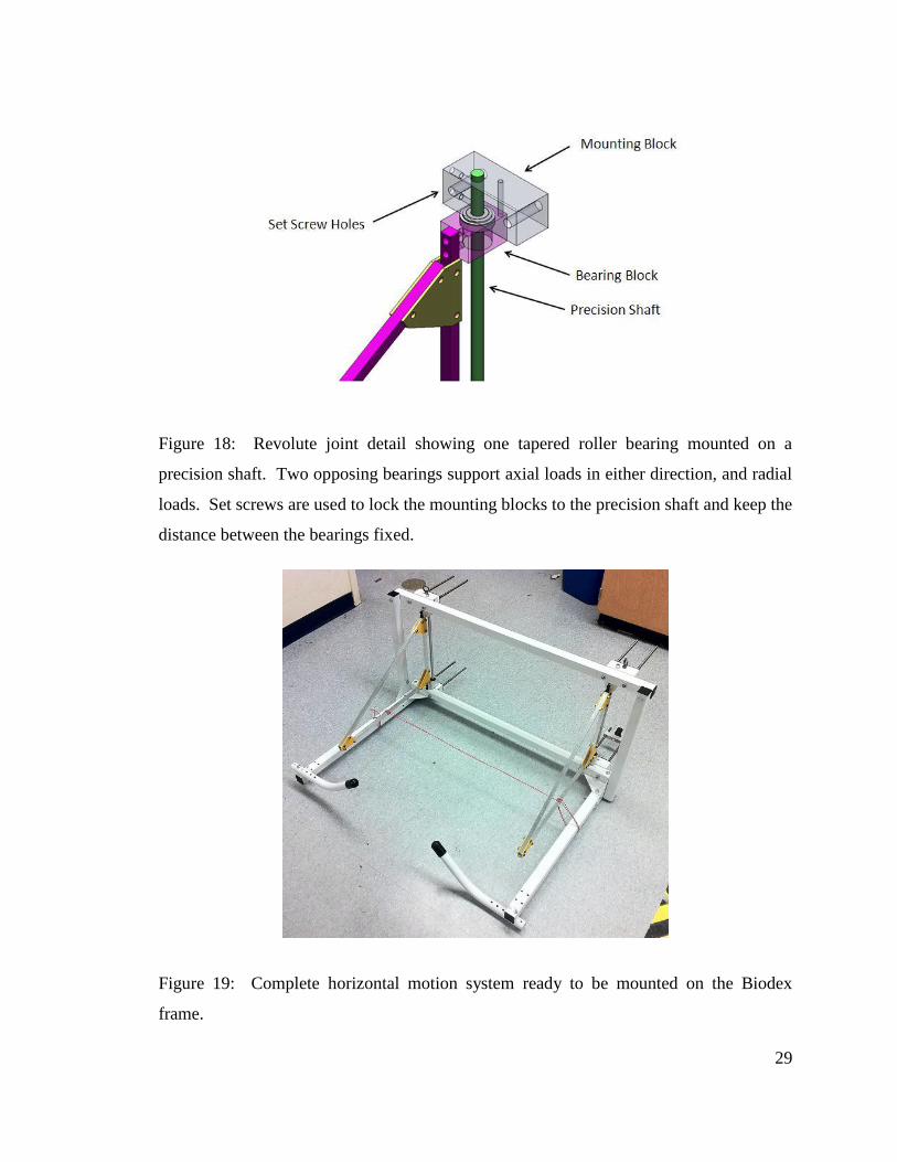
Figure 18: Revolute joint detail showing one tapered roller bearing mounted on a precision shaft. Two opposing bearings support axial loads in either direction, and radial loads. Set screws are used to lock the mounting blocks to the precision shaft and keep the distance between the bearings fixed. ........................................................................................ 29
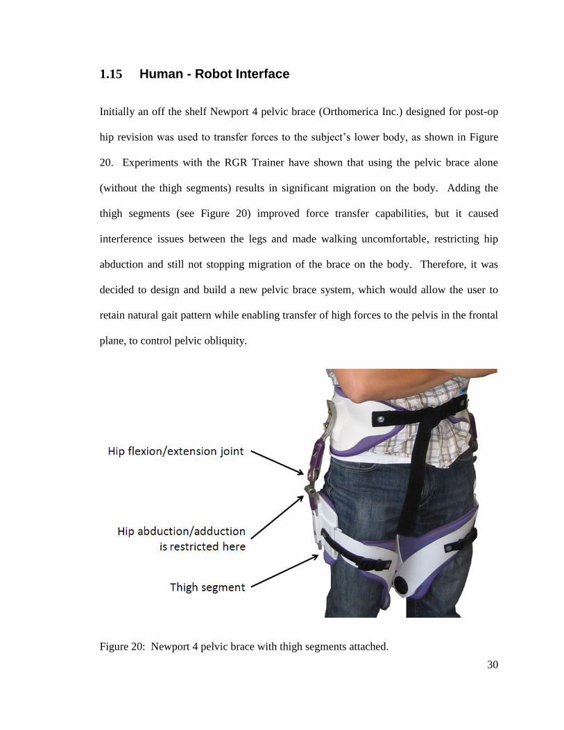
Figure 19: Complete horizontal motion system ready to be mounted on the Biodex frame. ....................... 29 Figure 20: Newport 4 pelvic brace with thigh segments attached. .............................................................. 30 Figure 21: LOPES DOFs, including free hip flexion/extension and free abduction/adduction. ..................... 32 Figure 22: BLEEX worn by a user. ................................................................................................................. 33 Figure 23: Pelvic brace design of BLEEX exoskeleton. ................................................................................... 33 Figure 24: Complete human-robot interface suspended from the RGR Trainer’s actuation system –
front view. ................................................................................................................................. 34 Figure 25: HRI top view. Plastic shells wrap around subject’s pelvis. .......................................................... 35 Figure 26: Right side of the human-robot interface, with all DOFs (left) and adjustments (right)
shown. Plastic shell interfacing with subject’s waist was removed for clarity. The DOF axes are: (1) hip flexion, (2) hip abduction, (3) hip internal/external rotation, (4) knee flexion, (5) ankle flexion. Adjustments: (a) hip joint span, (b) pelvis width, (c) thigh length, (d) shank length, (e) knee frontal plane angle. .................................................... 36
viii
Figure 27: Hip revolute joint, with potentiometer for flexion-extension angle measurement. Precision shaft is double supported by a pair of needle pin bearings and thrust bearings. .................................................................................................................................... 37
Figure 28: Knee joints with adjustable frontal plane angle (two extremes shown) and rotary potentiometer for knee flexion/extension measurement. The design is optimized to resist moments in the frontal plane, resulting from force fields applied to pelvic obliquity. .................................................................................................................................... 38
Figure 29: Basic outline of impedance control architecture. Proportional and derivative gains (PD) produce a force command which is executed by the force loop with gain G. System’s interaction force with the environment (Fext) is measured with load cell. .................. 41
Figure 30: Simple model of actuator’s thrust rod. ........................................................................................ 42 Figure 31: Actuator shaft and force control law. .......................................................................................... 42 Figure 32: Dynamics of the actuator. ........................................................................................................... 43 Figure 33: Physical implementation of equation (4.14). ............................................................................... 45 Figure 34: The unconditioned load cell signal contains significant noise. .................................................... 47 Figure 35: Once analog – filtered, the noise level in the signal is greatly reduced. ...................................... 48 Figure 36: Unfiltered load cell signal – sinusoidal loading at 1Hz. ............................................................... 48 Figure 37: Low – pass analog – filtered (480Hz cutoff) load cell signal – sinusoidal loading at 1Hz. ........... 49 Figure 38: Combination of analog – filtering to remove high frequency aliases, and digital
filtering produces a clean force signal. ...................................................................................... 50 Figure 39: Xenus servo amplifier from Copley Controls Inc. ......................................................................... 51 Figure 40: Outline of the inner current loop contained in the Xenus servo amplifier. .................................. 51 Figure 41: Actuator shaft coupled to the body via pelvic brace, with load cell reading the
interaction forces....................................................................................................................... 53
Figure 42: In open loop mode, we see about 15-20% steady state error. .................................................... 54 Figure 43: Closed loop step response with proportional gain G=1. .............................................................. 55 Figure 44: Closed loop step response. With a proportional gain of 1.8, serious instability
occurred. .................................................................................................................................... 55 Figure 45: Linear motion impedance controller was used in bench testing. ................................................ 57 Figure 46: Position error (Des. Position – Act. Position) generated the force command (Fvirt). Load
cell measured actual interaction force (Fext). ............................................................................. 60 Figure 47: The addition of damping attenuated the oscillatory force interaction. Effects of
stiction can be seen just past maxima and minima. .................................................................. 60 Figure 48: Higher gain value caused greater environment deflection (Act. Position). Lack of
damping resulted in oscillatory response. ................................................................................. 61 Figure 49: After the damping ratio (zeta) was introduced, the oscillatory behavior diminished. ................ 61 Figure 50: At this high virtual stiffness setting, slight vibrations were again felt, and can be seen
in the Fext signal. ........................................................................................................................ 62 Figure 51: Increasing the damping ratio to 0.8 amplified the vibrations. .................................................... 63 Figure 52: Obliquity angle can be calculated knowing vertical position of the two attachment
points. D is the length of the direct line between the two attachment points, and y is the distance between them in the vertical direction. ................................................................ 65
Figure 53: The PD controller acts on the obliquity error and outputs the appropriate force command. Low pass filters 1 and 2 are RC anti-alias filters. .................................................... 66
Figure 54: Details of the PD gain block from Figure 53. The proportional gain Kc is specified at the obliquity level, while the derivative gain Bc acts on linear velocity error at the actuator level. Bc is computed from Kc (linear motion equivalent) and the specified damping ratio ζ using Equation 4.17. Velocity feedback undergoes secondary filtering (after velocity error is computed). ............................................................................... 66
Figure 55: Conceptual diagram and synchronization algorithm diagram, adapted from [6]. ...................... 68 Figure 56: Foot switch construction. Clear plastic sheet taped over the top improves user
comfort. ..................................................................................................................................... 69
ix
Figure 57: MATLAB’s “unwrap” function produces continuous curves of periodic time series. The range of phase angle of 5 radians to 75 radians covers approx. 11 full gait cycles. ................. 70
Figure 58: With offset introduced to remove delay, heel strikes as predicted by gait estimation algorithm (“Trep”) nearly coincide with those produced by the discrete gait event (heel strike). ........................................................................................................................................ 71
Figure 59: Overall Control System Architecture. ........................................................................................... 72 Figure 60: Two consecutive gait cycles. Synchronization algorithm output predicts left heel
strikes well, and gives good estimate of gait cycle location mid-stride. Gait estimation (Synchr Output) is the progression through the gait cycle from 0 to 1 (100%). Force field activation sigmoid switch (3Hz) was set to go on at 44% and off at 76%. Heel strike is marked by the rising edge of the ‘Heel Strike Switch’ signal. ................. 73
Figure 61: Layout of hardware components of the RGR Trainer’s control system. ...................................... 74 Figure 62: Interaction force data with the RGR Trainer’s control system set to ‘follow’ mode,
under two force gain settings, collected at 50Hz. ..................................................................... 75 Figure 63: Backdrivability test results (with force control gains as indicated). The healthy subject
ambulated at his comfortable walking speed (CWS) of 3km/h. Approximately 50% (6dB) interaction force reduction for frequencies 0-6Hz can be seen........................................ 76
Figure 64: Bandwidth test setup with two compression springs (k=5.66kN/m). .......................................... 77 Figure 65: Commanded force (Chirp Force Command) and the resulting interaction force. ........................ 78 Figure 66: Actuator force bandwidth test results. ........................................................................................ 79 Figure 67: Analog amplifier-enable safety circuit. ........................................................................................ 81 Figure 68: Pelvic obliquity trajectories collected from healthy and impaired subjects in the study
by Cruz et al. [44]. The impaired subjects (stroke) clearly exhibit a hip-hiking pelvic motion trajectory. ...................................................................................................................... 88
Figure 69: Graphical representation of protocol 1. ...................................................................................... 89 Figure 70: Result of hip-hike inducing test. The interaction force magnitudes measured by the
load cell (Fint) are graphed. Models fitted to the data (Fit) were used to estimate time constants. .................................................................................................................................. 91
Figure 71: Graphical representation of protocol 2. ...................................................................................... 95 Figure 72: Sample result from one subject tested under Protocol 2. In the top graph, refBL is the
baseline pelvic obliquity of the subject, refHH is the hip-hiking trajectory from Cruz et.al, actBL is the mean pelvic obliquity trajectory under force field, actHH is the average hip-hiking trajectory produced by the subject under force field and actAE is the average pelvic obliquity following hip-hike training session. In the bottom graph, pelvic obliquity curves from all gait cycles in epoch 4 are shown (dashed blue) along with baseline (solid black). Here one gait cycle spans between consecutive left foot toe-offs. ..................................................................................................................................... 96
Figure 73: Subject # 2 baseline and hip-hiking plots. Baseline and its standard deviation curves are plotted along with their inverses (with first half of gait cycle plotted first, and vice versa) in order to aid in visualizing symmetry. Right hip-hike curves are also inverted and plotted in reverse order to facilitate comparison with left hip-hike curves. ....................... 98
Figure 74: Subject # 3 baseline and hip-hiking plots..................................................................................... 99 Figure 75: Subject # 4 baseline and hip-hiking plots..................................................................................... 99 Figure 76: Subject # 7 baseline and hip-hiking plots................................................................................... 100 Figure 77: Subject # 8 baseline and hip-hiking plots................................................................................... 100 Figure 78: Mean pelvic left hip-hike obliquities of 8 subjects (across ca. 200 gait cycles) and mean
across the means of 7 subjects (subject # 2 data excluded due to the time-series’ extreme mismatch with the rest due to erroneous foot switch operation). ............................ 102
Figure 79: Graphical representation of protocol 3 trial. A session consisted of five such trials concatenated into a single run. Epoch 1 was only used in trial 1 of the run, and each trial used a different force field magnitude. ............................................................................ 106
x
Figure 80: Taking into account the offset in pelvic obliquity between baseline (refBL) and pelvic obliquities resulting from hip-hike training, an after-effect can be observed (actAE-Early) which diminishes with time (actAE-Late). .................................................................................... 107
Figure 81: Subject 2 exhibits significant after-effect, characterized by exaggerated pelvic drop at the beginning of the third epoch (backdrive), labeled as actAE-Early. This after-effect diminishes throughout the duration of the third epoch, and the de-adapt epoch (4
th)
seems to accomplish its task (actde-Adapt). ................................................................................ 108 Figure 82: This subject’s baseline pelvic obliquity (refBL) has a gross offset. Nevertheless, the
action of the RGR Trainer does make the subject produce a hip-hike during the second half of the gait cycle. Unlike what was observed in Figure 80 and 81, the subject exhibits a reduced pelvic drop, which returns to baseline over time. ......................... 109
Figure 83: Graphical representation of a single trial of protocol 4. A complete session consisted of three trials running continuously (each using a different force field), with trial 2 and 3 consisting of epochs 2 through 5. Epoch 3 type was randomized. Two sessions per training type (assistive or resistive) were run to ensure that every combination of force field and epoch 3 type was tested. ................................................................................. 113
Figure 84: Assistive training: baseline trajectories and pelvic obliquities during epoch 2 (train at Kc = 5N-m/deg) followed by epoch 3b (backdrive, check-). Subjects hip-hiked during the training period, and exaggerated pelvic drop in the subsequent epoch may indicate motor adaptation. ..................................................................................................... 114
Figure 85: Assistive training: baseline trajectories and pelvic obliquities during epoch 2 (train at 15N-m/deg) followed by epoch 3b (backdrive, check-). Subjects hip-hiked during the training period. The exaggerated pelvic drop in the subsequent epoch (3b) may be a sign of motor adaptation. ....................................................................................................... 115
Figure 86: Assistive training: baseline trajectories and pelvic obliquities during epoch 2 (train at 25N-m/deg) followed by epoch 3b (backdrive, check-). Subject 2 exhibited most exaggerated pelvic drop in epoch 3b. ...................................................................................... 116
Figure 87: Similarity of pelvic obliquity to hip-hiking reference (0-300 strides, training at 5N-m/deg) and to baseline reference (301-600 strides, epoch 3b) during assistive training. ................................................................................................................................... 117
Figure 88: Similarity of pelvic obliquity to hip-hiking reference (0-300 strides, training at 15N-m/deg) and to baseline reference (301-600 strides, epoch 3b) during assistive training. Only subject 4 exhibited a gait pattern close to hip-hiking for several gait cycles after the switch occurred. ............................................................................................. 118
Figure 89: Similarity of pelvic obliquity to hip-hiking reference (0-300 strides, training at 25N-m/deg) and to baseline reference (301-600 strides, epoch 3b) during assistive training. ................................................................................................................................... 119
Figure 90: Resistive training: baseline trajectories and pelvic obliquities during epoch 2 (train at 5N-m/deg) followed by epoch 3b (backdrive-check). .............................................................. 120
Figure 91: Resistive training: baseline trajectories and pelvic obliquities during epoch 2 (train at 15N-m/deg) followed by epoch 3b (backdrive-check). ............................................................ 121
Figure 92: Resistive training: baseline trajectories and pelvic obliquities during epoch 2 (train at 25N-m/deg) followed by epoch 3b (backdrive-check). ............................................................ 122
Figure 93: Resistive training at 5N-m/deg: Interaction forces during epoch 2 (Hip Hike), epoch 3b (Backdrive), and epoch 4 (Error Clamp). .................................................................................. 123
Figure 94: Resistive training at 15N-m/deg: Interaction forces during epoch 2 (Hip Hike), epoch 3b (Backdrive), and epoch 4 (Error Clamp). Subject 1 resisted the force field the most, peaking at almost 100N (mean), and during the Error Clamp epoch he again fought against the system the most (-40N mean). This particular subject reported verbally during the training session having difficulty recalling his baseline pelvic obliquity pattern. .................................................................................................................................... 124
xi
Figure 95: Resistive training at 25N-m/deg: Interaction forces during epoch 2 (Hip Hike), epoch 3b (Backdrive), and epoch 4 (Error Clamp). ............................................................................. 125
Figure 96: Position error (Des. Position – Act. Position) generated the force command (Fvirt). Load cell measured actual interaction force (Fext). ........................................................................... 132
Figure 97: The addition of damping attenuated the oscillatory force interaction. Effects of stiction can be seen just past maxima and minima. ................................................................ 133
Figure 98: Higher gain value caused greater environment deflection (Act. Position). Lack of damping again resulted in oscillatory response. ..................................................................... 133
Figure 99: Once again, after the damping ratio (zeta) was introduced, the oscillatory behavior diminished. .............................................................................................................................. 134
Figure 100: At this high virtual stiffness setting, slight vibrations were again felt, and can be seen in the Fext signal. ...................................................................................................................... 134
Figure 101: Again, with the damping ratio increased, the vibrations diminish. ......................................... 135 Figure 102: As the damping ratio was increased to 0.6, undesirable behavior appeared. The
virtual damper component of the command signal began displaying vibratory behavior. The resulting forces were felt by the subject, but are not present in the measured force signal Fext due to low-pass filtering. ............................................................... 135
Figure 103: With the reference trajectory of 3Hz and no damping, the measured force signal (Fext) tended to lag behind the commanded force (Fvirt). .................................................................. 136
Figure 104: Increase in damping ratio smoothed out both force curves. ................................................... 136 Figure 105: With the damping ratio set to 0.5, the system still behaved well. .......................................... 137 Figure 106: Once the damping ratio was increased to 0.6, the performance deteriorated due to
appearance of high frequency vibrations, which can be seen in the Fvirt signal, and could be felt by the subject. ..................................................................................................... 137
Figure 107: With the reference trajectory frequency increased to 6Hz, actuator thrust rod’s inertia caused significant distortions to the position and force profiles. The system still behaved in a stable manner. ............................................................................................. 138
Figure 108: Introduction of damping had the effect of correcting the profile of the external measured force Fext, by properly modulating the virtual force Fvirt. ......................................... 138
Figure 109: Inertial effects cause the measured force profile Fext to lag significantly behind position error. .......................................................................................................................... 139
Figure 110: Increasing the damping ratio seemed to make the controller efforts (Fvirt) more abrupt. ..................................................................................................................................... 139
Figure 111: As seen before, damping ratio of 0.6 amplified the derivative action of the PD impedance controller. This caused high frequency vibrations. ............................................... 140
Figure 112: Subject 1 – 2nd
trial. ................................................................................................................. 141 Figure 113: Subject 1 – 3rd trial. ................................................................................................................. 142 Figure 114: Subject 1 – 4th trial. ................................................................................................................. 142 Figure 115: Subject 1 – 1st trial. ................................................................................................................. 143 Figure 116: Subject 1 – 5
th trial. .................................................................................................................. 143
Figure 117: Subject 2 – 5th
trial. .................................................................................................................. 144 Figure 118: Subject 2 – 2
nd trial. ................................................................................................................. 144
Figure 119: Subject 2 – 1st
trial. .................................................................................................................. 145 Figure 120: Subject 2 – 3
rd trial. .................................................................................................................. 145
Figure 121: Subject 2 – 4th
trial. .................................................................................................................. 146 Figure 122: Subject 3 – 1
st trial. .................................................................................................................. 146
Figure 123: Subject 3 – 2nd
trial. ................................................................................................................. 147 Figure 124: Subject 3 – 3
rd trial. .................................................................................................................. 147
Figure 125: Subject 3 – 4th
trial. .................................................................................................................. 148 Figure 126: Subject 3 – 5
th trial. .................................................................................................................. 148
Figure 127: Control link optimized for mass. .............................................................................................. 151
xii
Figure 128: Concept 2 with torsion bar applying moments in pelvic obliquity and two push-rods in pelvic rotation, here pictured with two Copley linear actuators. ............................................ 152
Figure 129: Constant-radius arc guided by bearings used to place the center of rotation within the subject’s body. ................................................................................................................... 153
Figure 130: The gimbals at the hip joints allow for hip abduction/adduction and flexion/extension. Flexible transmission is required to apply moments at pelvic obliquity. .................................................................................................................................. 154
Figure 131: RGR Trainer 2DOF actuation concept. ..................................................................................... 155 Figure 132: Actuator mount – detail design. .............................................................................................. 156 Figure 133: Closed linkage mechanism. ..................................................................................................... 157 Figure 134: Top view of the mechanism. .................................................................................................... 158 Figure 135: Definition of pelvic obliquity Φ and pelvic rotation θ angles. Pelvic brace as viewed
from behind. ............................................................................................................................ 159 Figure 136: Forces fL and fR necessary to produce desired net forces and moments. ................................. 160 Figure 137: Force f resolved into the component magnitudes and unit vectors. ....................................... 162 Figure 138: RGR Trainer 2DOF frame structure only. BWS beam is reinforced with steel cables. ............. 164 Figure 139: Side view of RGR Trainer 2DOF over treadmill. Manipulators are shown attached to
pelvic interface worn by 99th
percentile female subject. ......................................................... 164 Figure 140: Manipulator attachment to frame. ......................................................................................... 165 Figure 141: Handle bar tilt adjustment using quick release clamps and spring loaded plunger. ............... 165 Figure 142: Handle bar height adjustment. ................................................................................................ 166

xiii
List of Tables
Table 1: Summary of hip-hike data. The means exclude subject # 2 data. Only one subject (#6) was left-foot-dominant. .......................................................................................................... 101

xiv
Glossary
Afferent - anatomical term: towards the center of the body
Brain plasticity - the capacity of the nervous system to change its structure
and network, neurogenesis, its cognition and function
over a lifetime
Central Pattern Generators - neural networks that produce rhythmic patterned outputs
without sensory feedback
Contralateral - side of the body opposite to the side of brain lesion;
generally this side of the body is the one affected by
stroke
Equinus - condition characterized by tiptoe walking on one or both
feet. It is usually associated with clubfoot
Hemiparesis - weakness on one side of the body
Ipsilateral - same side of the body as the side of brain lesion;
generally this side of the body is not affected by the
stroke
Motor adaptation - modification of a movement from trial to trial based on
error feedback
Motor cortex - region of the cerebral cortex involved in the planning,
control, and execution of voluntary motor functions
Motor learning - formation of new motor pattern that occurs via long-term
practice (i.e. days, weeks, years)
Neurorehabilitation - complex medical process which aims to aid recovery
from nervous system injury, and to minimize and/or
compensate for any functional alterations resulting from
it
Orthosis - orthopedic appliance or apparatus used to support, align,
prevent, or correct deformities or to improve function of
movable parts of the body

1
Introduction
1.1 Problem Description
Each year 800,000 people suffer a stroke in the United States alone [1]. Stroke is a
leading cause of disability. Stroke survivors experience weakness and difficulties
moving one side of the body (i.e. they are affected by hemiparesis), with a negative effect
on the performance of motor activities such as walking. Walking allows individuals to
perform activities of daily living [2, 3]. The ability to walk is strongly correlated with
quality of life [4]. Hemiparesis and abnormal synergy patterns are characteristic of gait
disorders following stroke. Abnormal synergy patterns include equinus synergy, paretic
synergy and reflex coactivation [5]. Comfortable walking speed is reduced in stroke
survivors. Asymmetries mark post-stroke ambulation. Asymmetry of stance time during
gait, a common feature following stroke, often limits walking efficiency, results in
instability, and causes an aesthetically sub-optimal gait pattern. Therefore, the restoration
of a normal gait pattern is an important goal of post-stroke rehabilitation.
1.2 Significance
Many rehabilitation approaches have been used to promote functional recovery in stroke
survivors. Unfortunately, the rehabilitation process is labor intensive, since it often relies
on a one-to-one administration of therapy, i.e. clinicians work with a single patient at a
time. Robotic systems for gait retraining have been recently developed to facilitate the
administration of intensive therapy. Most of the existing systems focus on the correction
2
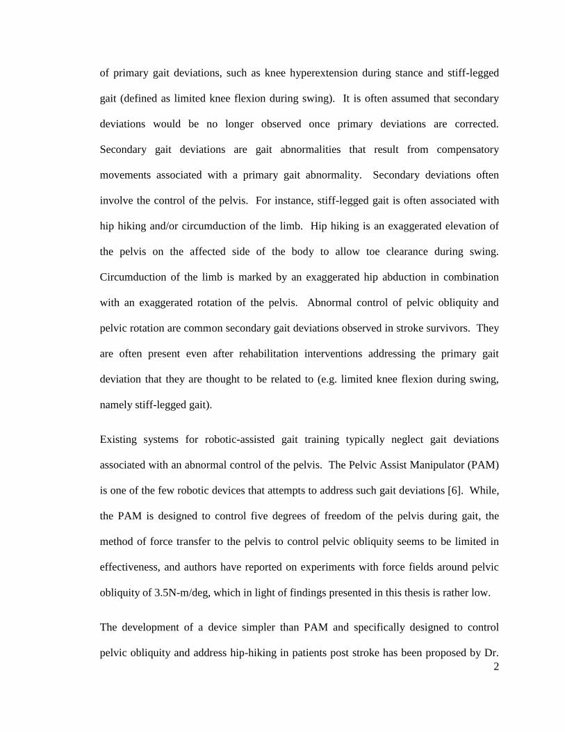
of primary gait deviations, such as knee hyperextension during stance and stiff-legged
gait (defined as limited knee flexion during swing). It is often assumed that secondary
deviations would be no longer observed once primary deviations are corrected.
Secondary gait deviations are gait abnormalities that result from compensatory
movements associated with a primary gait abnormality. Secondary deviations often
involve the control of the pelvis. For instance, stiff-legged gait is often associated with
hip hiking and/or circumduction of the limb. Hip hiking is an exaggerated elevation of
the pelvis on the affected side of the body to allow toe clearance during swing.
Circumduction of the limb is marked by an exaggerated hip abduction in combination
with an exaggerated rotation of the pelvis. Abnormal control of pelvic obliquity and
pelvic rotation are common secondary gait deviations observed in stroke survivors. They
are often present even after rehabilitation interventions addressing the primary gait
deviation that they are thought to be related to (e.g. limited knee flexion during swing,
namely stiff-legged gait).
Existing systems for robotic-assisted gait training typically neglect gait deviations
associated with an abnormal control of the pelvis. The Pelvic Assist Manipulator (PAM)
is one of the few robotic devices that attempts to address such gait deviations [6]. While,
the PAM is designed to control five degrees of freedom of the pelvis during gait, the
method of force transfer to the pelvis to control pelvic obliquity seems to be limited in
effectiveness, and authors have reported on experiments with force fields around pelvic
obliquity of 3.5N-m/deg, which in light of findings presented in this thesis is rather low.
The development of a device simpler than PAM and specifically designed to control
pelvic obliquity and address hip-hiking in patients post stroke has been proposed by Dr.
3
Paolo Bonato, the director of the Motion Analysis Lab at Spaulding Rehabilitation
Hospital in Boston, and Assistant Professor at Harvard Medical School. The result is a
robotic device of low mechanical complexity, presented in this thesis, which allows all
the natural motions of the pelvis, while being able to selectively and compliantly guide
the pelvis in the frontal plane (pelvic obliquity) in order to target hip-hiking in patients
post stroke. This device uses impedance control and human-machine synchronization to
generate corrective forces as a response to deviations from pre-determined pelvic
obliquity trajectories. The corrective force fields are applied onto the subject via a lower
body exoskeleton, which can very effectively transfer forces to the pelvis, while its 10
DOFs allow for unhindered ambulation on the treadmill.
1.3 Contributions
The main contributions of this thesis are:
- A novel design and actuation method of a robotic device, which applies forces to
the pelvic area in order to affect the pelvic obliquity angle during ambulation.
- The novel design of a lower body exoskeleton, which can effectively and reliably
transfer moments to the pelvis in the frontal plane.
- A control method, which facilitates application of determinate moment onto the
pelvis in frontal plane with a single actuator.
- Demonstration of feasibility of inducing the learning of new gait patterns via
application of force fields to pelvic obliquity.
Some of the work presented in this thesis has been the subject of the following
publications:
4
- Pietrusinski M., Cajigas I., Bonato P. and Mavroidis C., "Healthy Subject Testing
with the Robotic Gait Rehabilitation(RGR) Trainer,” Proceedings of the CISM-
IFToMM Symposium on Robot Design, Dynamics, and Control, June 12 – 15,
2012.
- Pietrusinski M., Cajigas I., Bonato P. and Mavroidis C., "Robotic Gait
Rehabilitation Trainer Pelvic Obliquity Trajectory Recording with Robotic Gait
Rehabilitation (RGR) Trainer and Lower Body Exoskeleton,” Proceedings of the
Dynamic Walking Conference (DWC), May 21 – May 24, 2012.
- Pietrusinski, Maciej; Unluhisarcikli, Ozer; Mavroidis, Constantinos; Cajigas,
Iahn; Bonato, Paolo; , "Design of human — Machine interface and altering of
pelvic obliquity with RGR Trainer," Rehabilitation Robotics (ICORR), 2011 IEEE
International Conference on , vol., no., pp.1-6, June 29 2011-July 1 2011.
- Pietrusinski, M.; Cajigas, I.; Goldsmith, M.; Bonato, P.; Mavroidis, C.; ,
"Robotically generated force fields for stroke patient pelvic obliquity gait
rehabilitation," Robotics and Automation (ICRA), 2010 IEEE International
Conference on , vol., no., pp.569-575, 3-7 May 2010.
- Pietrusinski, M.; Cajigas, I.; Mizikacioglu, Y.; Goldsmith, M.; Bonato, P.;
Mavroidis, C.; , "Gait Rehabilitation therapy using robot generated force fields
applied at the pelvis," Haptics Symposium, 2010 IEEE , vol., no., pp.401-407,
25-26 March 2010.
Submitted:
- Pietrusinski M., Severini G., Cajigas I., Bonato P. and Mavroidis C., "Design of a
gait training device for control of pelvic obliquity," submitted for possible
5
presentation in Engineering in Medicine & Biology (EMBC), 2012 IEEE
International Conference on, August 28 – September 1, 2012.
- Pietrusinski M., Cajigas I., Severini G., Bonato P. and Mavroidis C., "Robotic
Gait Rehabilitation Trainer," submitted for possible publication in the IEEE /
ASME Transactions on Mechatronics, March, 2012.
In preparation:
- IEEE Transactions on Neural Systems and Rehabilitation Engineering, June,
2012
As a result of this work, two provisional patent applications have been filed:
- Pietrusinski M., Mavroidis C., "Mobile Wearable Orthopedic Lower Body
Exoskeleton for Control of Pelvic Obliquity during Gait," Invention Disclosure
submitted on November 30, 2011 (INV-1234). Initial provisional patent
application filed on December 5, 2011.
- Pietrusinski M., Mavroidis C., Bonato P., Unluhisarcikli O., Cajigas I., Weinberg
B., "Orthopedic Lower Body Exoskeleton for Torque Transfer to Control
Rotation of Pelvis during Gait," Invention disclosure submitted on May 31, 2011
(INV-1148). Initial provisional patent application filed on June 24, 2011.
The publication presented at the International Conference on Robotics and Automation
(ICRA 2010) was also nominated for the best medical robotics paper award.
6
1.4 Overview
This thesis is an attempt to address several questions. In Chapter 2 the current state of the
art compliantly controlled robotic devices for gait rehabilitation are presented. Chapter 3
describes the design of a robotic device of low mechanical complexity such that it can
reliably and effectively apply force fields to pelvic motion in the frontal plane (pelvic
obliquity) when walking on a treadmill. Chapter 4 presents how to control The RGR
Trainer such that it can generate the prescribed corrective force fields, and finally in
Chapter 5 several experimental protocols are tested on healthy subjects, providing insight
on the many challenges and the right approaches for gait retraining by application of
force fields at the pelvis.
7
Background
1.5 Human Gait
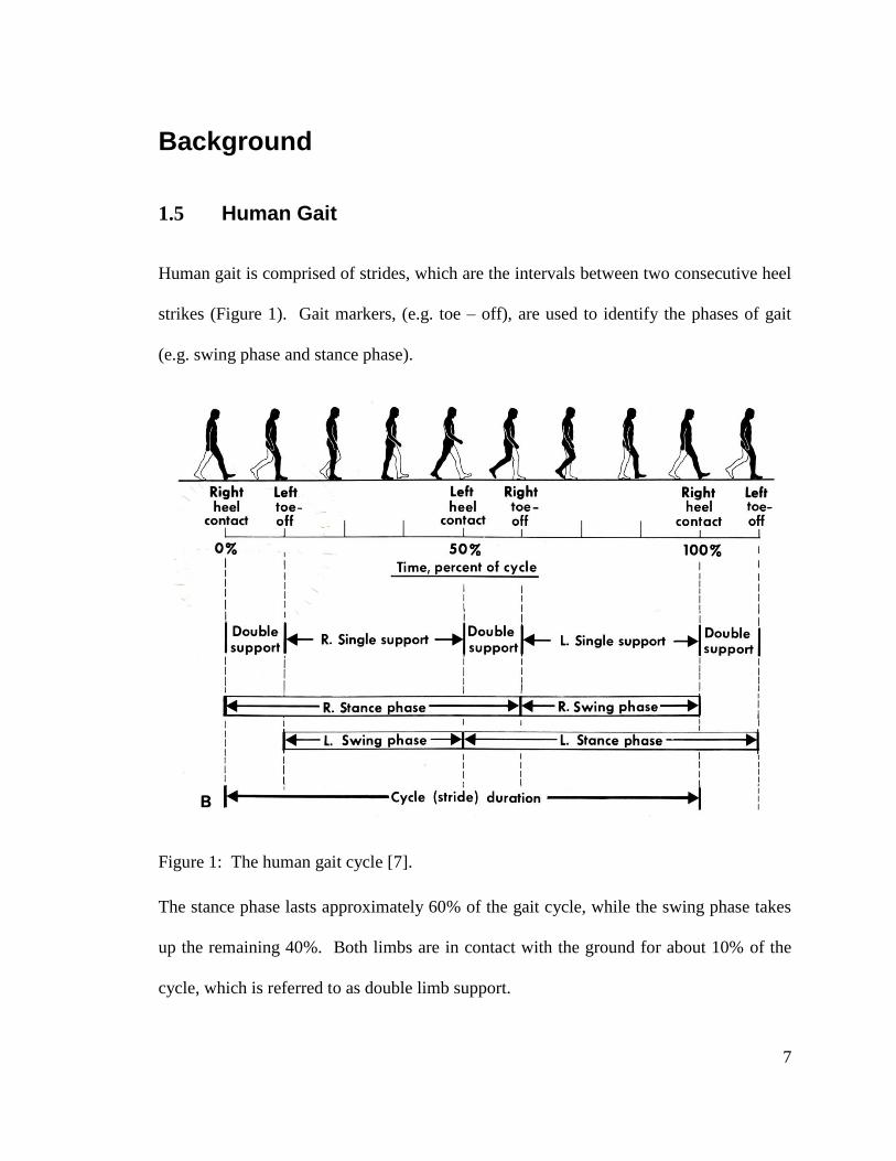
Human gait is comprised of strides, which are the intervals between two consecutive heel
strikes (Figure 1). Gait markers, (e.g. toe – off), are used to identify the phases of gait
(e.g. swing phase and stance phase).
Figure 1: The human gait cycle [7].
The stance phase lasts approximately 60% of the gait cycle, while the swing phase takes
up the remaining 40%. Both limbs are in contact with the ground for about 10% of the
cycle, which is referred to as double limb support.
8
1.6 Pelvis Motion during Gait
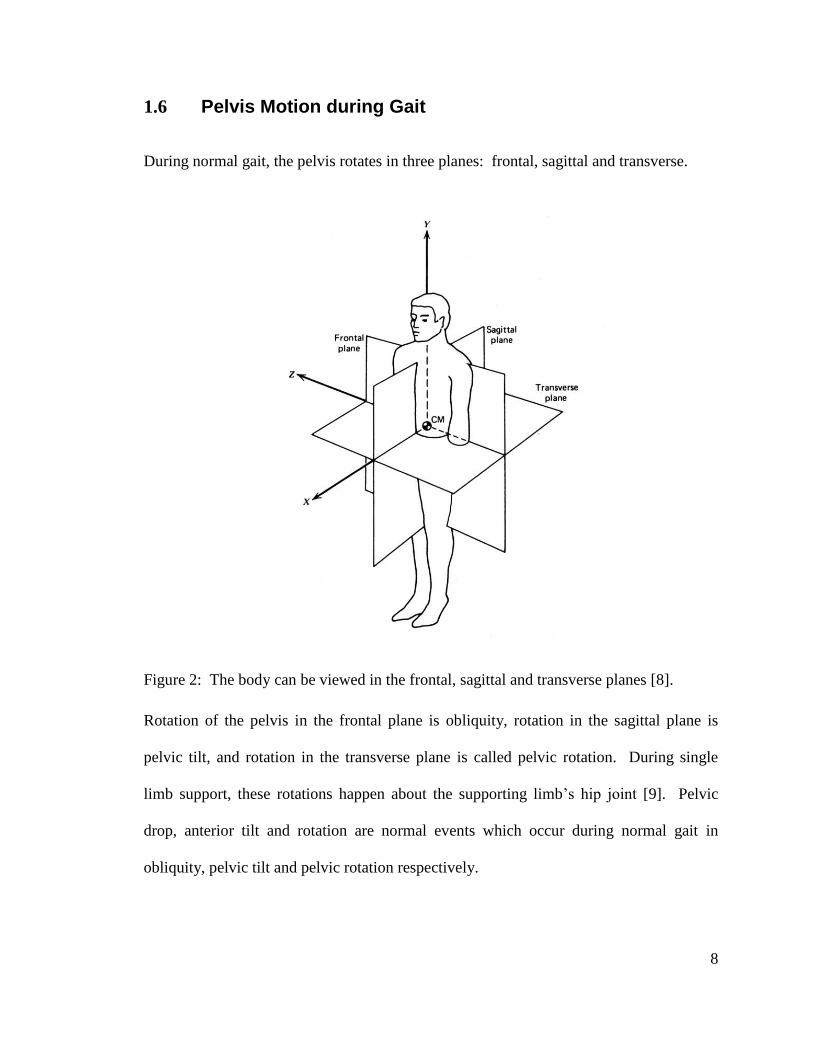
During normal gait, the pelvis rotates in three planes: frontal, sagittal and transverse.
Figure 2: The body can be viewed in the frontal, sagittal and transverse planes [8].
Rotation of the pelvis in the frontal plane is obliquity, rotation in the sagittal plane is
pelvic tilt, and rotation in the transverse plane is called pelvic rotation. During single
limb support, these rotations happen about the supporting limb’s hip joint [9]. Pelvic
drop, anterior tilt and rotation are normal events which occur during normal gait in
obliquity, pelvic tilt and pelvic rotation respectively.

9
Figure 3: Normal pelvis motion events in gait [9].
1.7 Common Gait Deviations in Pelvic Motion
The most common primary gait deviation in patients post – stroke is stiff – legged gait.
This gait deviation oftentimes results in the subject employing secondary gait deviations
which involve motor control of the pelvis. Stiff legged gait is associated with hip-hiking
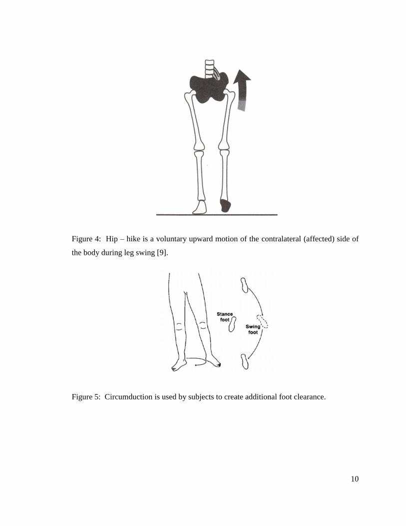
(Figure 4) or circumduction (Figure 5). Hip-hiking is an exaggerated elevation of the
pelvis on the contralateral side (i.e. hemiparetic side) to allow toe clearance during swing,
while circumduction is an exaggerated rotation of the pelvis in combination with an
exaggerated hip abduction. Abnormal control of pelvic obliquity and rotation of the
pelvis are the most common secondary gait deviations observed in post-stroke patients.
A subject will employ these secondary gait deviations in order to assist in foot clearance
when either hip flexion or knee flexion are inadequate [9].
10
Figure 4: Hip – hike is a voluntary upward motion of the contralateral (affected) side of
the body during leg swing [9].
Figure 5: Circumduction is used by subjects to create additional foot clearance.
11
1.8 Gait Rehabilitation
Animal research studies have shown that goal oriented, repetitive training is the primary
means of augmenting post-stroke motor relearning [10]. Human clinical trial studies that
utilize goal-oriented, repetitive, active training such as constrained induced movement
therapy [11], partial weight-supported ambulation [12] and robotic therapy [13] have
demonstrated encouraging results. Based on the growing body of scientific evidence
pointing to the effectiveness of goal-oriented motor retraining, clinicians have recently
privileged a goal-oriented approach also in gait retraining, and have utilized treadmills to
implement clinical protocols. Studies examining treadmill gait retraining have shown its
effectiveness in improving walking velocity and other key characteristics of ambulation
[12, 14] and a positive effect on mobility. Treadmill walking is used as a substitute to
level ground walking since not only it appears to be an effective clinical tool, but also it
offers some practical advantages over level ground gait retraining. For instance,
treadmill gait retraining uses less space and is relatively simple to apply this technique in
less functional patients with the use of weight support. Studies have shown that walking
on a treadmill does not significantly change the gait pattern compared to level ground
waking [14] and that improvements achieved during treadmill gait retraining transfer to
level ground walking. In cases when patients are unable to properly ambulate, use of a
treadmill for gait retraining makes it easier for physical therapists to administer motion to
lower extremities manually (Figure 6).
12
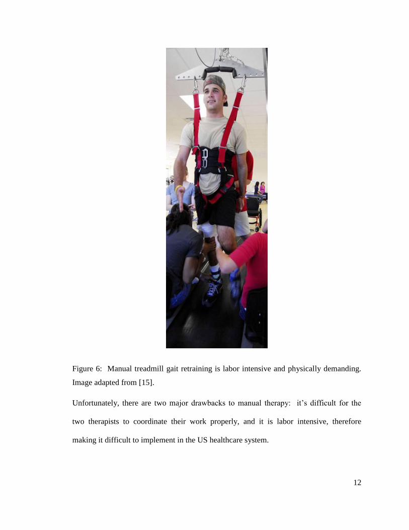
Figure 6: Manual treadmill gait retraining is labor intensive and physically demanding.
Image adapted from [15].
Unfortunately, there are two major drawbacks to manual therapy: it’s difficult for the
two therapists to coordinate their work properly, and it is labor intensive, therefore
making it difficult to implement in the US healthcare system.
13
1.9 Robotic Gait Rehabilitation
Due to the difficulties associated with manual gait retraining, robotic gait retraining
systems have been developed to facilitate administration of intensive gait retraining
therapy. From the point of view of training strategy and robot control, there are two
types of robotic devices for rehabilitation: those which drive the body components in
position mode regardless of patient efforts, and those which apply force-fields to the
body, therefore modulating the forces applied onto the body depending on patient’s
efforts. The latter method, employing force-fields, has been shown to be the preferred
method for retraining post-stroke subjects to regain their motor functions [16].
Therefore, only those robotic devices, which apply force-fields (with force measurement)
to the lower body for the purpose of gait retraining, are presented here.
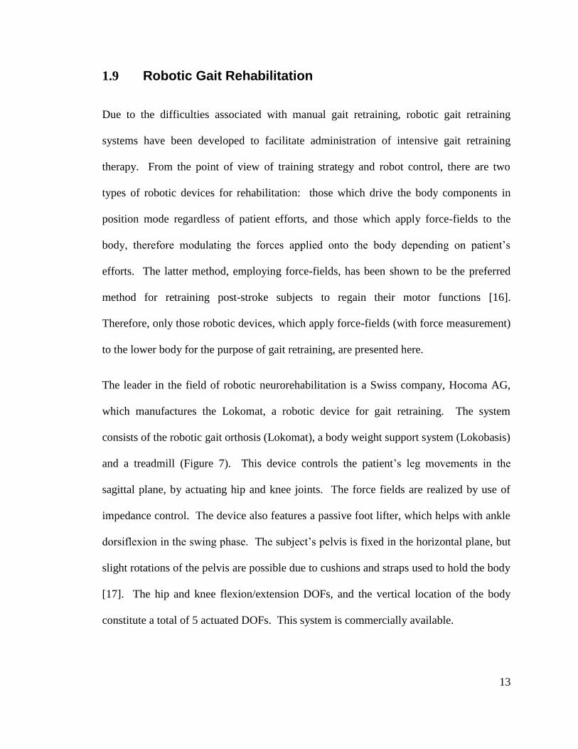
The leader in the field of robotic neurorehabilitation is a Swiss company, Hocoma AG,
which manufactures the Lokomat, a robotic device for gait retraining. The system
consists of the robotic gait orthosis (Lokomat), a body weight support system (Lokobasis)
and a treadmill (Figure 7). This device controls the patient’s leg movements in the
sagittal plane, by actuating hip and knee joints. The force fields are realized by use of
impedance control. The device also features a passive foot lifter, which helps with ankle
dorsiflexion in the swing phase. The subject’s pelvis is fixed in the horizontal plane, but
slight rotations of the pelvis are possible due to cushions and straps used to hold the body
[17]. The hip and knee flexion/extension DOFs, and the vertical location of the body
constitute a total of 5 actuated DOFs. This system is commercially available.
14
Figure 7: The Lokomat in action [18].
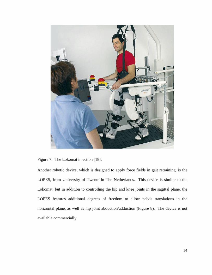
Another robotic device, which is designed to apply force fields in gait retraining, is the
LOPES, from University of Twente in The Netherlands. This device is similar to the
Lokomat, but in addition to controlling the hip and knee joints in the sagittal plane, the
LOPES features additional degrees of freedom to allow pelvis translations in the
horizontal plane, as well as hip joint abduction/adduction (Figure 8). The device is not
available commercially.
15
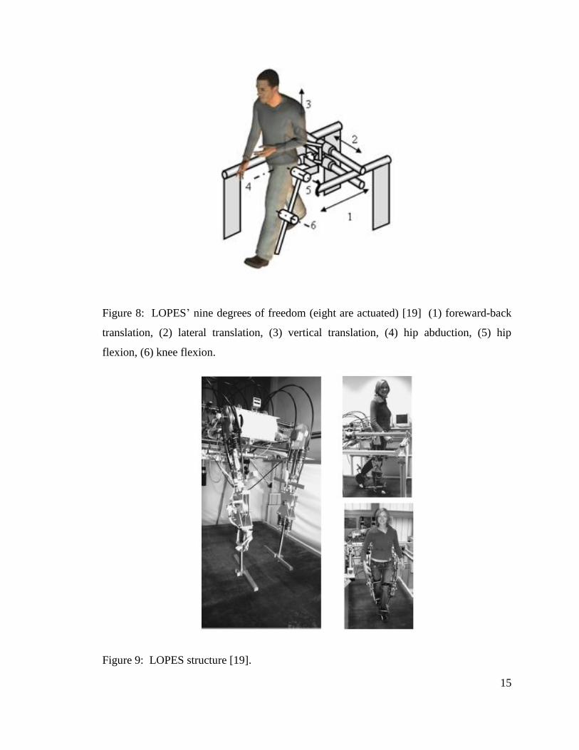
Figure 8: LOPES’ nine degrees of freedom (eight are actuated) [19] (1) foreward-back
translation, (2) lateral translation, (3) vertical translation, (4) hip abduction, (5) hip
flexion, (6) knee flexion.
Figure 9: LOPES structure [19].
16
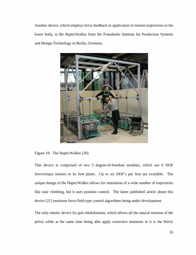
Another device, which employs force feedback in application of motion trajectories to the
lower body, is the HapticWalker from the Fraunhofer Institute for Production Systems
and Design Technology in Berlin, Germany.
Figure 10: The HapticWalker [20].
This device is comprised of two 3 degree-of-freedom modules, which use 6 DOF
force/torque sensors in its foot plates. Up to six DOF’s per foot are available. The
unique design of the HapticWalker allows for simulation of a wide number of trajectories
like stair climbing, but it uses position control. The latest published article about this
device [21] mentions force-field type control algorithms being under development.
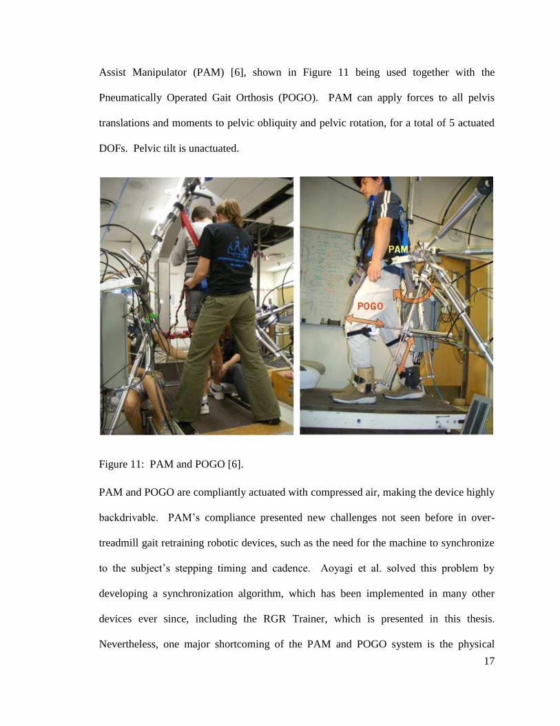
The only robotic device for gait rehabilitation, which allows all the natural motions of the
pelvis while at the same time being able apply corrective moments to it is the Pelvic
17
Assist Manipulator (PAM) [6], shown in Figure 11 being used together with the
Pneumatically Operated Gait Orthosis (POGO). PAM can apply forces to all pelvis
translations and moments to pelvic obliquity and pelvic rotation, for a total of 5 actuated
DOFs. Pelvic tilt is unactuated.
Figure 11: PAM and POGO [6].
PAM and POGO are compliantly actuated with compressed air, making the device highly
backdrivable. PAM’s compliance presented new challenges not seen before in over-
treadmill gait retraining robotic devices, such as the need for the machine to synchronize
to the subject’s stepping timing and cadence. Aoyagi et al. solved this problem by
developing a synchronization algorithm, which has been implemented in many other
devices ever since, including the RGR Trainer, which is presented in this thesis.
Nevertheless, one major shortcoming of the PAM and POGO system is the physical
18
interface between the robot and the human, as the authors point out. Moments are
applied to the pelvis via a semi-rigid belt, and the POGO which is not directly linked
mechanically to the pelvic belt exerts flexion/extension moments at the hips and knees.
The authors reported on conducting tests with spinal cord injury patients, where the force
fields which PAM was configured to generate around pelvic obliquity and pelvic rotation
were 200N-m/rad (3.5N-m/deg), which is quite low.
1.10 Conclusion
The Lokomat, the LOPES and the HapticWalker systems described above have the
capability to correct primary gait deviations, such as knee hyperextension during stance
and stiff legged gait defined as limited knee flexion during swing, but the secondary gait
deviations in the pelvis are not targeted. PAM is the only device for gait retraining which
allows all natural motions of the pelvis and can apply moments to the pelvis, but its
performance seems to be limited by the design of the physical interface between the robot
and the subject.
The development of the RGR Trainer was proposed by Dr. Paolo Bonato, to facilitate
robotic gait retraining using force-fields applied to the secondary gait deviations in the
pelvic motion. The RGR Trainer allows all of the natural motions of the pelvis, and
features a lower body exoskeleton which employs the waist, thighs, shanks and feet to
transfer moments to the pelvis. The mechanical design of the RGR Trainer coupled with
the lower body exoskeleton, highly backdrivable linear actuator, impedance control and
PAM’s synchronization algorithm produced a gait retraining device which can effectively
and reliably apply corrective moments to pelvic obliquity. These features make the RGR

19
Trainer arguably the best robotic system for studying motor control of pelvic obliquity in
healthy subjects, which may lead to developing better gait retraining therapies for
patients post-stroke.
20
On the Mechanical Design of RGR Trainer
1.11 Introduction
Neurorehabilitation, whether in upper or lower limbs, puts forth certain desirable
qualities, which robotic devices should possess, such as high backdrivability and force
controllability [6]. Some devices have been developed with these qualities in mind [22-
24]. On the other hand the Lokomat was first designed as a position-controlled device,
and only later was it outfitted with impedance control, in order to improve its
performance [25]. In light of this, the actuation system and the human-robot interface of
the RGR Trainer were designed to be simple, with low moving mass and low friction,
easing the task of the control system in generating appropriate performance of the overall
system.
1.12 RGR Trainer Working Principle
The RGR Trainer is a stationary device, which is placed over a treadmill, and which
generates force fields around the user’s pelvis, while they ambulate on the treadmill, in
order to administer gait retraining therapy. The particular secondary gait deviation,
which the RGR Trainer targets in patients post-stroke, is hip-hiking. Hip-hiking occurs
when the leg affected by hemiparesis is in swing phase. During that period, the weight of
the body is supported by the other leg (ipsilateral side).
21
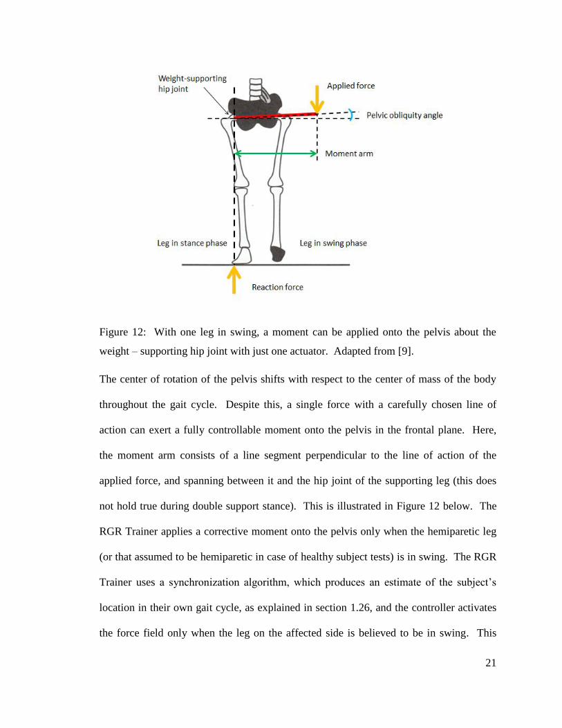
Figure 12: With one leg in swing, a moment can be applied onto the pelvis about the
weight – supporting hip joint with just one actuator. Adapted from [9].
The center of rotation of the pelvis shifts with respect to the center of mass of the body
throughout the gait cycle. Despite this, a single force with a carefully chosen line of
action can exert a fully controllable moment onto the pelvis in the frontal plane. Here,
the moment arm consists of a line segment perpendicular to the line of action of the
applied force, and spanning between it and the hip joint of the supporting leg (this does
not hold true during double support stance). This is illustrated in Figure 12 below. The
RGR Trainer applies a corrective moment onto the pelvis only when the hemiparetic leg
(or that assumed to be hemiparetic in case of healthy subject tests) is in swing. The RGR
Trainer uses a synchronization algorithm, which produces an estimate of the subject’s
location in their own gait cycle, as explained in section 1.26, and the controller activates
the force field only when the leg on the affected side is believed to be in swing. This
22
makes it possible to use only one actuator to generate a well-defined moment around the
pelvis in the frontal plane, with a vertical reaction force at the support leg, which is equal
in magnitude to the applied force generated by the actuator.
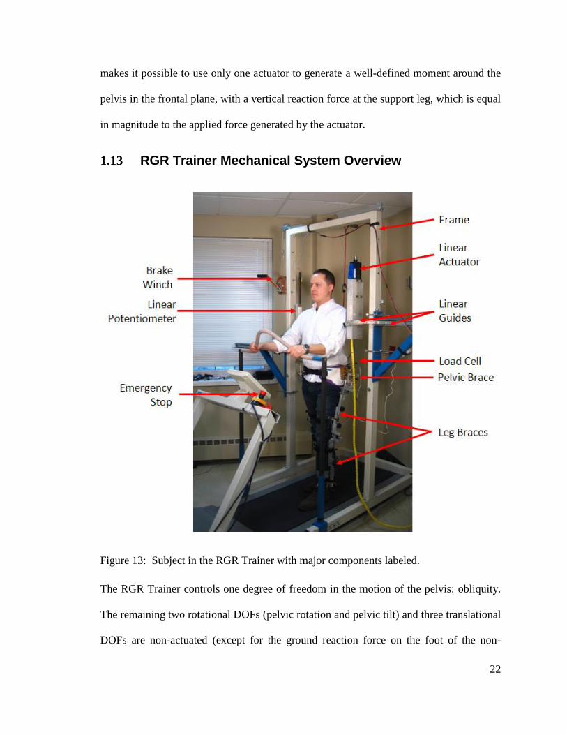
1.13 RGR Trainer Mechanical System Overview
Figure 13: Subject in the RGR Trainer with major components labeled.
The RGR Trainer controls one degree of freedom in the motion of the pelvis: obliquity.
The remaining two rotational DOFs (pelvic rotation and pelvic tilt) and three translational
DOFs are non-actuated (except for the ground reaction force on the foot of the non-
23
actuated side). The two major mechanical subsystems of the RGR Trainer, as shown in
Figure 13 are:
1. Actuation system, which follows the natural motions of the subject’s pelvis, while
applying corrective moments to pelvic obliquity as determined by the control
system.
2. Human-robot interface (HRI), a lower body exoskeleton, which is designed to
transfer corrective moments to the pelvis. The HRI employs the waist, thighs,
shanks and feet to effectively and reliably impart significant forces onto the user’s
lower body, and alter the orientation of the pelvis in the frontal plane (pelvic
obliquity).
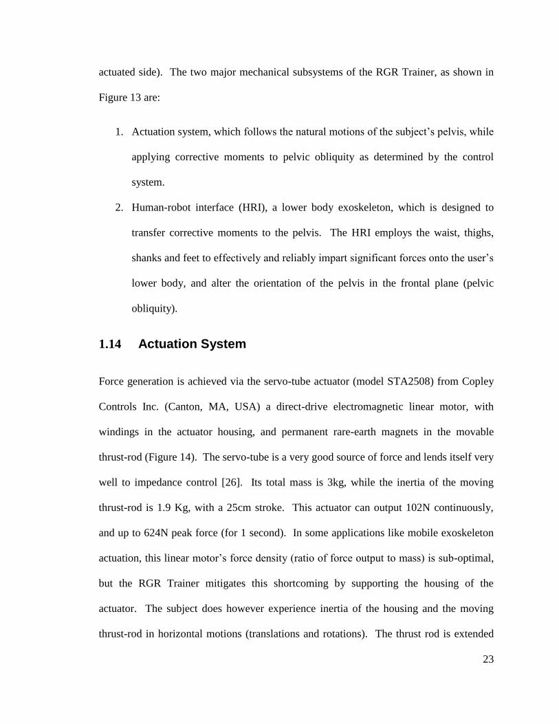
1.14 Actuation System
Force generation is achieved via the servo-tube actuator (model STA2508) from Copley
Controls Inc. (Canton, MA, USA) a direct-drive electromagnetic linear motor, with
windings in the actuator housing, and permanent rare-earth magnets in the movable
thrust-rod (Figure 14). The servo-tube is a very good source of force and lends itself very
well to impedance control [26]. Its total mass is 3kg, while the inertia of the moving
thrust-rod is 1.9 Kg, with a 25cm stroke. This actuator can output 102N continuously,
and up to 624N peak force (for 1 second). In some applications like mobile exoskeleton
actuation, this linear motor’s force density (ratio of force output to mass) is sub-optimal,
but the RGR Trainer mitigates this shortcoming by supporting the housing of the
actuator. The subject does however experience inertia of the housing and the moving
thrust-rod in horizontal motions (translations and rotations). The thrust rod is extended
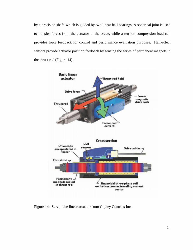
24
by a precision shaft, which is guided by two linear ball bearings. A spherical joint is used
to transfer forces from the actuator to the brace, while a tension-compression load cell
provides force feedback for control and performance evaluation purposes. Hall-effect
sensors provide actuator position feedback by sensing the series of permanent magnets in
the thrust rod (Figure 14).
Figure 14: Servo tube linear actuator from Copley Controls Inc.
25
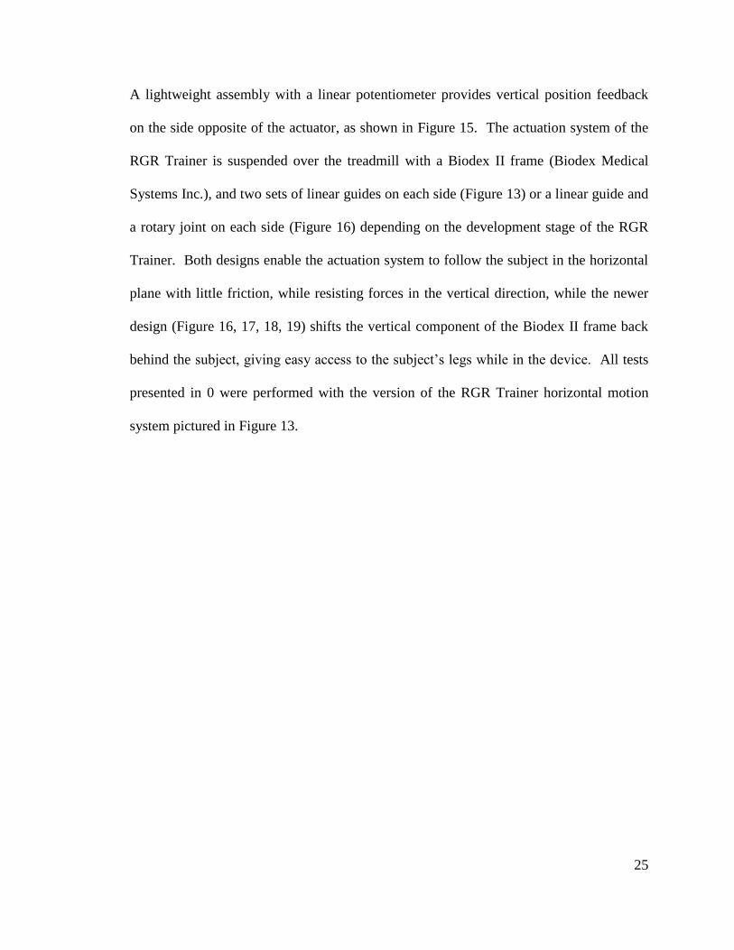
A lightweight assembly with a linear potentiometer provides vertical position feedback
on the side opposite of the actuator, as shown in Figure 15. The actuation system of the
RGR Trainer is suspended over the treadmill with a Biodex II frame (Biodex Medical
Systems Inc.), and two sets of linear guides on each side (Figure 13) or a linear guide and
a rotary joint on each side (Figure 16) depending on the development stage of the RGR
Trainer. Both designs enable the actuation system to follow the subject in the horizontal
plane with little friction, while resisting forces in the vertical direction, while the newer
design (Figure 16, 17, 18, 19) shifts the vertical component of the Biodex II frame back
behind the subject, giving easy access to the subject’s legs while in the device. All tests
presented in 0 were performed with the version of the RGR Trainer horizontal motion
system pictured in Figure 13.
26
Figure 15: Sensing (pelvis orientation and force) and actuation in the RGR Trainer. The
servo-tube actuator (which contains hall-effect sensor based internal position
measurement) and the linear potentiometer are fixed to the frame of the RGR Trainer, but
can follow the motion of the body in the horizontal plane.
27
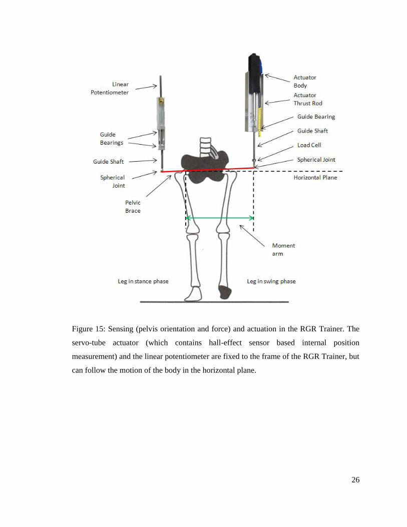
Figure 16: Horizontal motion system upgrade with the actuation system. Triangular
subassemblies support the linear actuator assembly and the linear potentiometer
assembly. A revolute joint about the vertical axis and a prismatic joint in the horizontal
plane provide unconstrained motion in the horizontal plane while constraining motion in
the vertical direction.
28
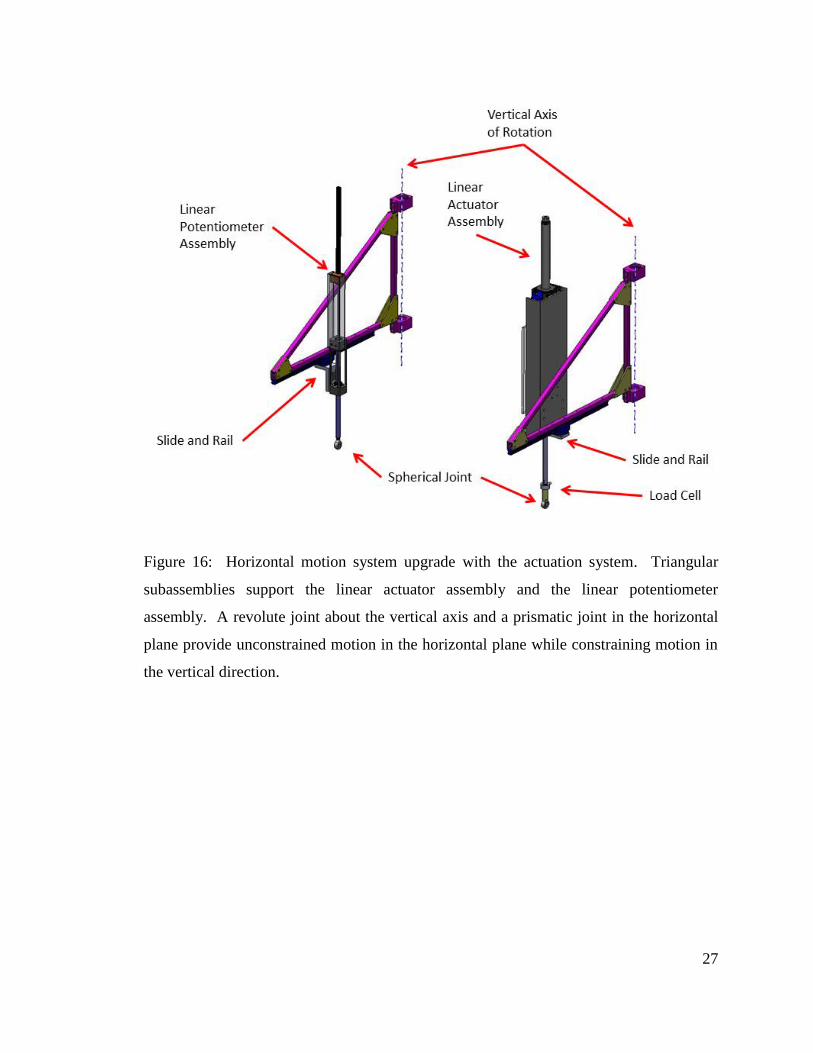
Figure 17: The horizontal motion system (upgrade) with the actuation system is secured
to the Biodex frame with four locking clamp subassemblies. Body weight support
components are not shown.
Each structure is supported with two tapered roller bearings, which themselves are
located concentrically with precision shafts. The mounting block shown in Figure 18 is
bolted directly to the Biodex frame upright.
29
Figure 18: Revolute joint detail showing one tapered roller bearing mounted on a
precision shaft. Two opposing bearings support axial loads in either direction, and radial
loads. Set screws are used to lock the mounting blocks to the precision shaft and keep the
distance between the bearings fixed.
Figure 19: Complete horizontal motion system ready to be mounted on the Biodex
frame.
30
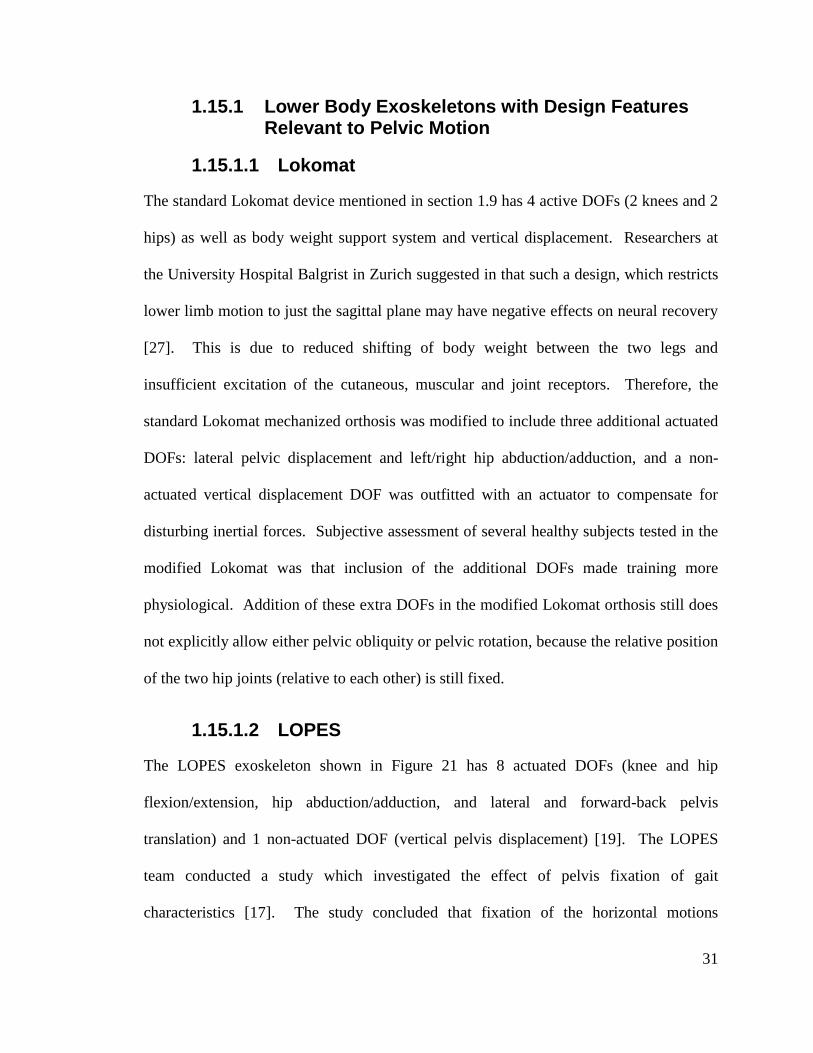
1.15 Human - Robot Interface
Initially an off the shelf Newport 4 pelvic brace (Orthomerica Inc.) designed for post-op
hip revision was used to transfer forces to the subject’s lower body, as shown in Figure
20. Experiments with the RGR Trainer have shown that using the pelvic brace alone
(without the thigh segments) results in significant migration on the body. Adding the
thigh segments (see Figure 20) improved force transfer capabilities, but it caused
interference issues between the legs and made walking uncomfortable, restricting hip
abduction and still not stopping migration of the brace on the body. Therefore, it was
decided to design and build a new pelvic brace system, which would allow the user to
retain natural gait pattern while enabling transfer of high forces to the pelvis in the frontal
plane, to control pelvic obliquity.
Figure 20: Newport 4 pelvic brace with thigh segments attached.
31
1.15.1 Lower Body Exoskeletons with Design Features Relevant to Pelvic Motion
1.15.1.1 Lokomat
The standard Lokomat device mentioned in section 1.9 has 4 active DOFs (2 knees and 2
hips) as well as body weight support system and vertical displacement. Researchers at
the University Hospital Balgrist in Zurich suggested in that such a design, which restricts
lower limb motion to just the sagittal plane may have negative effects on neural recovery
[27]. This is due to reduced shifting of body weight between the two legs and
insufficient excitation of the cutaneous, muscular and joint receptors. Therefore, the
standard Lokomat mechanized orthosis was modified to include three additional actuated
DOFs: lateral pelvic displacement and left/right hip abduction/adduction, and a non-
actuated vertical displacement DOF was outfitted with an actuator to compensate for
disturbing inertial forces. Subjective assessment of several healthy subjects tested in the
modified Lokomat was that inclusion of the additional DOFs made training more
physiological. Addition of these extra DOFs in the modified Lokomat orthosis still does
not explicitly allow either pelvic obliquity or pelvic rotation, because the relative position
of the two hip joints (relative to each other) is still fixed.
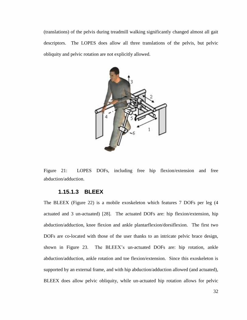
1.15.1.2 LOPES
The LOPES exoskeleton shown in Figure 21 has 8 actuated DOFs (knee and hip
flexion/extension, hip abduction/adduction, and lateral and forward-back pelvis
translation) and 1 non-actuated DOF (vertical pelvis displacement) [19]. The LOPES
team conducted a study which investigated the effect of pelvis fixation of gait
characteristics [17]. The study concluded that fixation of the horizontal motions
32
(translations) of the pelvis during treadmill walking significantly changed almost all gait
descriptors. The LOPES does allow all three translations of the pelvis, but pelvic
obliquity and pelvic rotation are not explicitly allowed.
Figure 21: LOPES DOFs, including free hip flexion/extension and free
abduction/adduction.
1.15.1.3 BLEEX
The BLEEX (Figure 22) is a mobile exoskeleton which features 7 DOFs per leg (4
actuated and 3 un-actuated) [28]. The actuated DOFs are: hip flexion/extension, hip
abduction/adduction, knee flexion and ankle plantarflexion/dorsiflexion. The first two
DOFs are co-located with those of the user thanks to an intricate pelvic brace design,
shown in Figure 23. The BLEEX’s un-actuated DOFs are: hip rotation, ankle
abduction/adduction, ankle rotation and toe flexion/extension. Since this exoskeleton is
supported by an external frame, and with hip abduction/adduction allowed (and actuated),
BLEEX does allow pelvic obliquity, while un-actuated hip rotation allows for pelvic
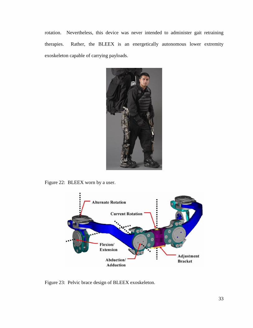
33
rotation. Nevertheless, this device was never intended to administer gait retraining
therapies. Rather, the BLEEX is an energetically autonomous lower extremity
exoskeleton capable of carrying payloads.
Figure 22: BLEEX worn by a user.
Figure 23: Pelvic brace design of BLEEX exoskeleton.
34
1.15.2 RGR Trainer’s Human-Robot Interface Design
1.15.2.1 General Description
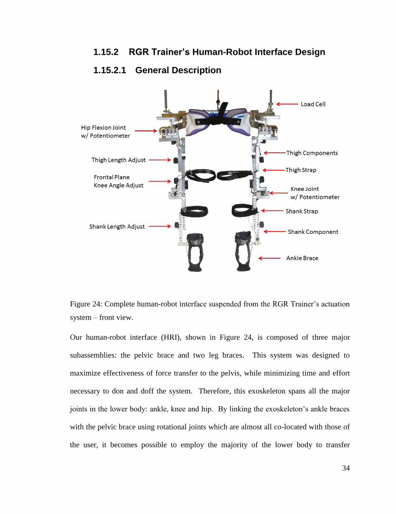
Figure 24: Complete human-robot interface suspended from the RGR Trainer’s actuation
system – front view.
Our human-robot interface (HRI), shown in Figure 24, is composed of three major
subassemblies: the pelvic brace and two leg braces. This system was designed to
maximize effectiveness of force transfer to the pelvis, while minimizing time and effort
necessary to don and doff the system. Therefore, this exoskeleton spans all the major
joints in the lower body: ankle, knee and hip. By linking the exoskeleton’s ankle braces
with the pelvic brace using rotational joints which are almost all co-located with those of
the user, it becomes possible to employ the majority of the lower body to transfer

35
moments to the pelvis. Also, strapping the human-robot interface to the relatively dense
feet solved the migration issue characteristic of the earlier method (Figure 20).
Two plastic shells (Newport 4 brace) wrap around the pelvis and locate the HRI with
respect to the body in the horizontal plane as shown in Figure 25.
Figure 25: HRI top view. Plastic shells wrap around subject’s pelvis.
1.15.2.2 Design Details
The human-robot interface has various free DOFs and adjustments to lower body size and
shape, as shown in Figure 26. Each half of the HRI explicitly accommodates 5 DOFs.
They are:
- hip abduction/adduction
- hip flexion/extension
- hip internal/external rotation
- knee flexion/extension
- ankle plantarflexion/dorsiflexion
36
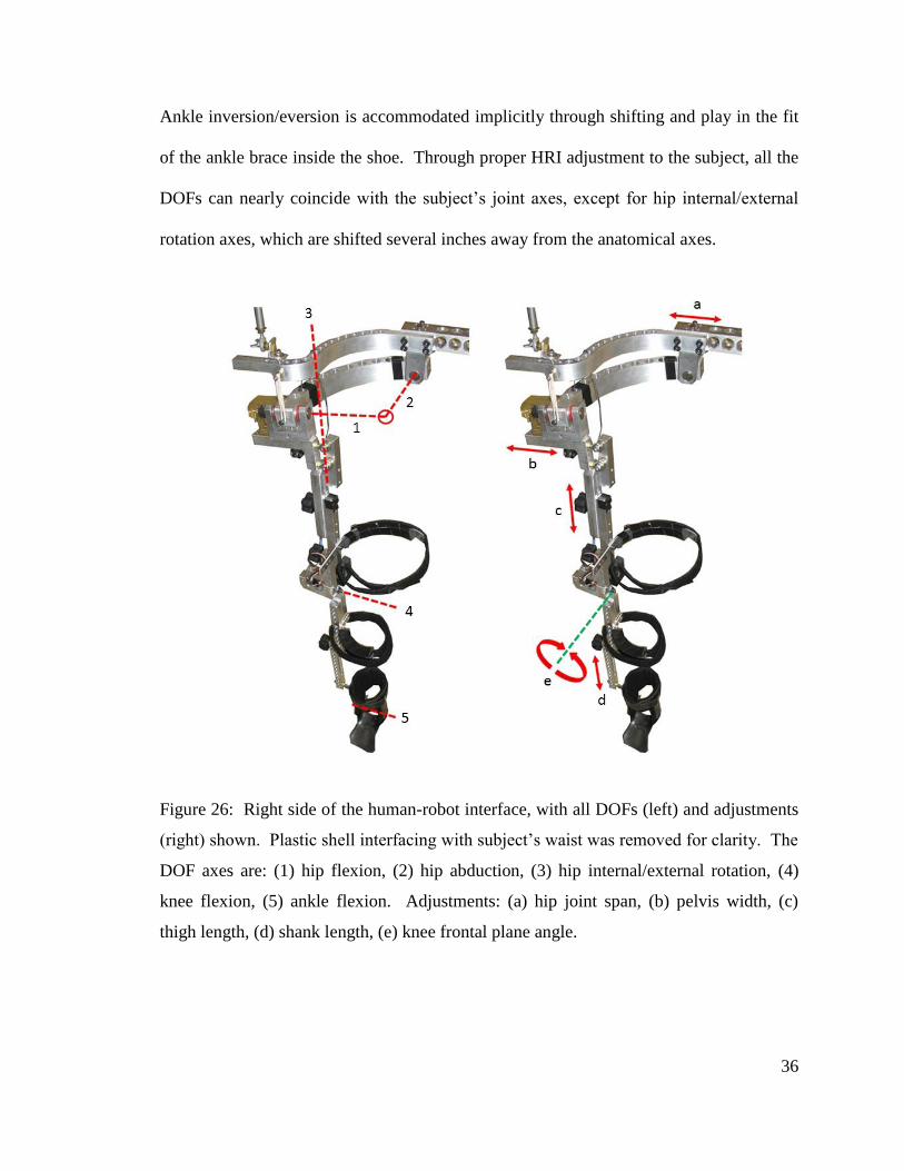
Ankle inversion/eversion is accommodated implicitly through shifting and play in the fit
of the ankle brace inside the shoe. Through proper HRI adjustment to the subject, all the
DOFs can nearly coincide with the subject’s joint axes, except for hip internal/external
rotation axes, which are shifted several inches away from the anatomical axes.
Figure 26: Right side of the human-robot interface, with all DOFs (left) and adjustments
(right) shown. Plastic shell interfacing with subject’s waist was removed for clarity. The
DOF axes are: (1) hip flexion, (2) hip abduction, (3) hip internal/external rotation, (4)
knee flexion, (5) ankle flexion. Adjustments: (a) hip joint span, (b) pelvis width, (c)
thigh length, (d) shank length, (e) knee frontal plane angle.
37
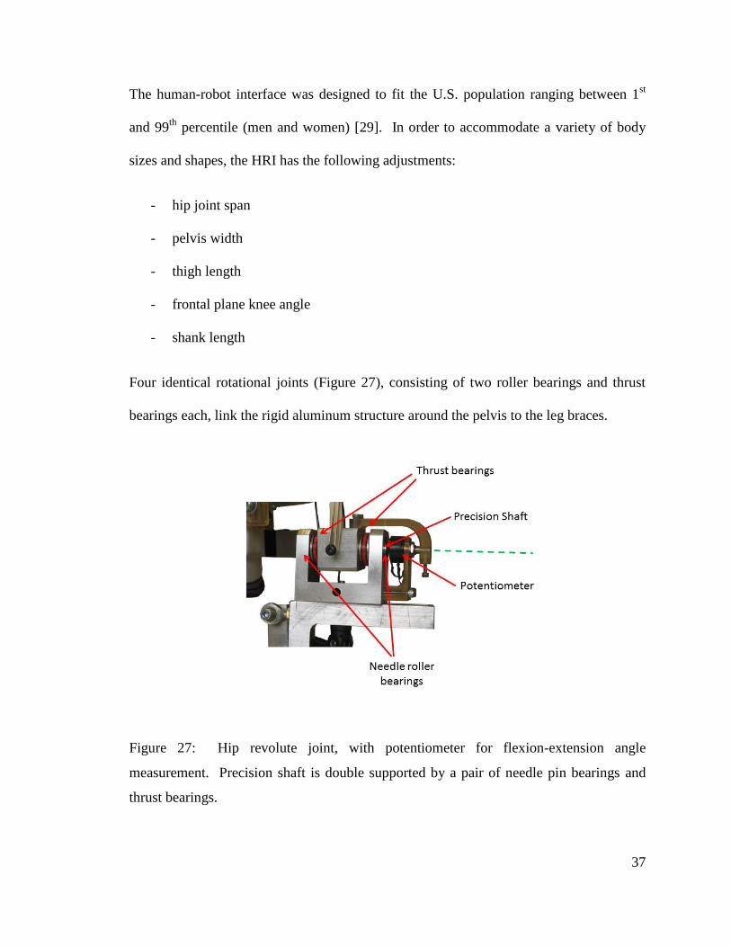
The human-robot interface was designed to fit the U.S. population ranging between 1st
and 99th
percentile (men and women) [29]. In order to accommodate a variety of body
sizes and shapes, the HRI has the following adjustments:
- hip joint span
- pelvis width
- thigh length
- frontal plane knee angle
- shank length
Four identical rotational joints (Figure 27), consisting of two roller bearings and thrust
bearings each, link the rigid aluminum structure around the pelvis to the leg braces.
Figure 27: Hip revolute joint, with potentiometer for flexion-extension angle
measurement. Precision shaft is double supported by a pair of needle pin bearings and
thrust bearings.
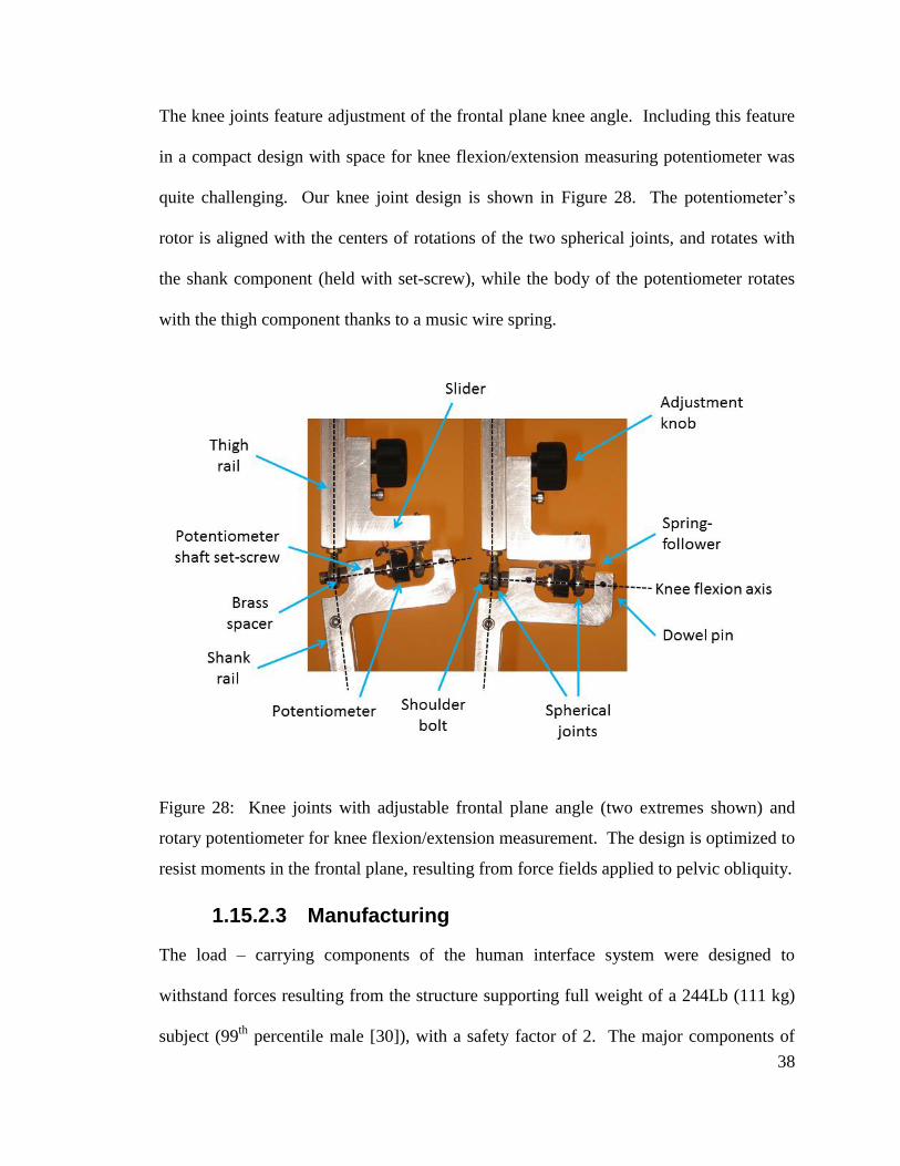
38
The knee joints feature adjustment of the frontal plane knee angle. Including this feature
in a compact design with space for knee flexion/extension measuring potentiometer was
quite challenging. Our knee joint design is shown in Figure 28. The potentiometer’s
rotor is aligned with the centers of rotations of the two spherical joints, and rotates with
the shank component (held with set-screw), while the body of the potentiometer rotates
with the thigh component thanks to a music wire spring.
Figure 28: Knee joints with adjustable frontal plane angle (two extremes shown) and
rotary potentiometer for knee flexion/extension measurement. The design is optimized to
resist moments in the frontal plane, resulting from force fields applied to pelvic obliquity.
1.15.2.3 Manufacturing
The load – carrying components of the human interface system were designed to
withstand forces resulting from the structure supporting full weight of a 244Lb (111 kg)
subject (99th
percentile male [30]), with a safety factor of 2. The major components of
39
the pelvic brace were machined from high strength aluminum alloy 7075. The
components which are subject to low forces were rapidly prototyped using an in-house
stereolithography (SLA) machine.
1.16 Conclusion
The final design of the RGR Trainer is a product of multiple revisions and updates, which
were motivated by continuous testing. The result is a practical, robust and reliable
design, which allows the user to ambulate with little restraint to all the natural lower body
joint articulations, while enabling transfer of high forces to the pelvis in the frontal plane
via the feet, shanks, and thighs.
40
RGR Trainer Control System
1.17 Introduction
The following sections outline various components of the control system which the RGR
Trainer employs to accurately and intelligently administer gait-retraining force fields to
the user.
1.18 Impedance Control Theory
Here, when speaking of impedance control, we refer to the control of the end-point
impedance of a robot or an actuator. Impedance control architecture consists of an inner
unity feedback force loop, and an outer unity feedback position loop. The main task of
the force loop is to increase backdrivability of the actuator. In that sense, force feedback
moves any actuator closer to an ideal source of force. The outer position loop sets the
relationship between the position of the end-effector, and the force it exerts. This is
usually accomplished with a PD controller, where the proportional term represents virtual
spring stiffness, and the derivative term acts like a virtual damper. A simple schematic of
an impedance controller is shown in Figure 29.
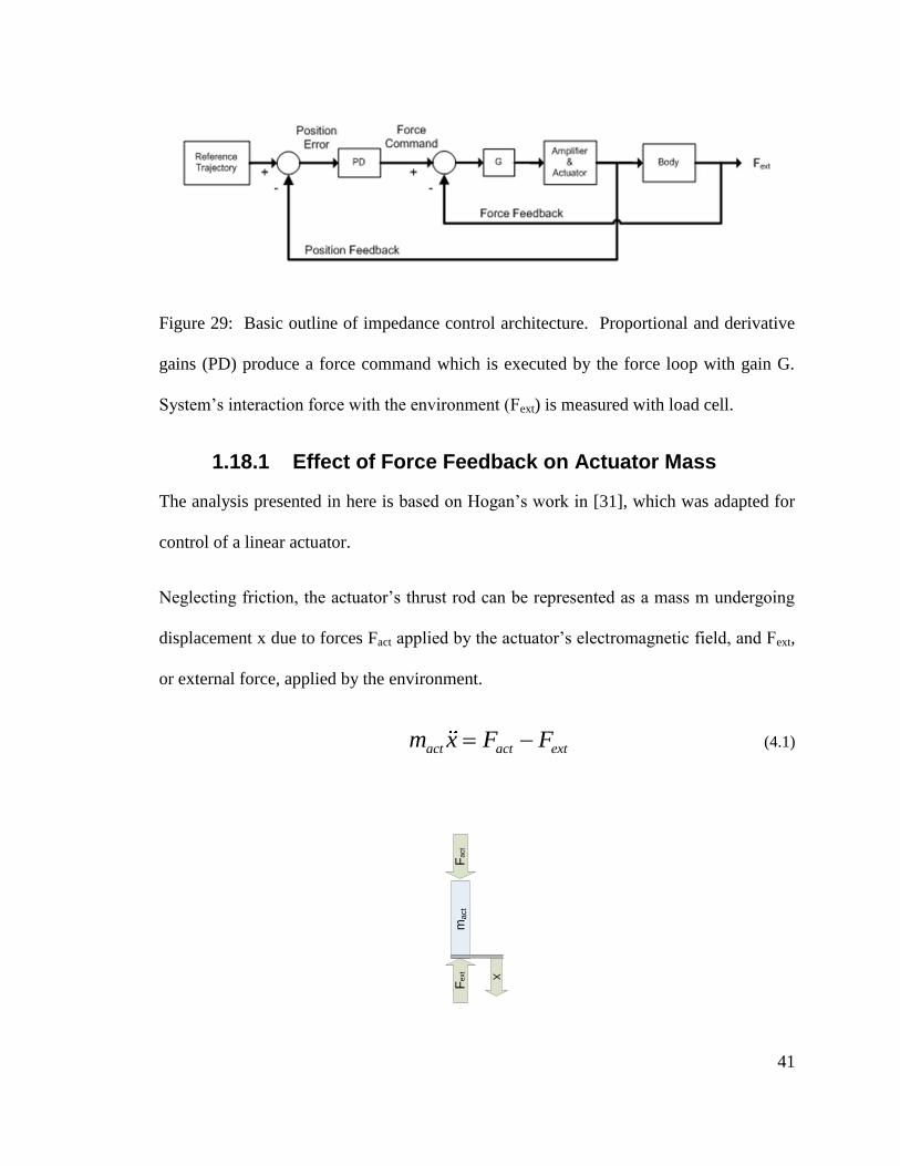
41
Figure 29: Basic outline of impedance control architecture. Proportional and derivative
gains (PD) produce a force command which is executed by the force loop with gain G.
System’s interaction force with the environment (Fext) is measured with load cell.
1.18.1 Effect of Force Feedback on Actuator Mass
The analysis presented in here is based on Hogan’s work in [31], which was adapted for
control of a linear actuator.
Neglecting friction, the actuator’s thrust rod can be represented as a mass m undergoing
displacement x due to forces Fact applied by the actuator’s electromagnetic field, and Fext,
or external force, applied by the environment.
act act extm x F F (4.1)
Fa
ct
Fe
xt
ma
ct
X
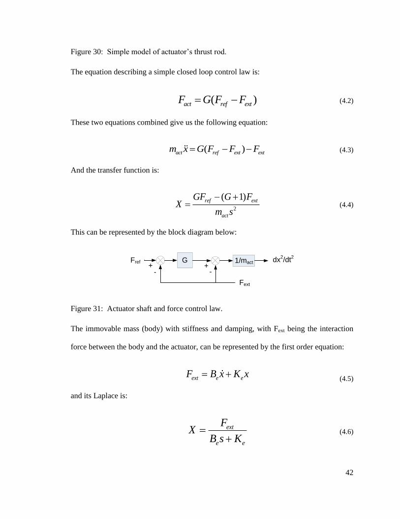
42
Figure 30: Simple model of actuator’s thrust rod.
The equation describing a simple closed loop control law is:
( )act ref extF G F F (4.2)
These two equations combined give us the following equation:
( )act ref ext extm x G F F F (4.3)
And the transfer function is:
2
( 1)ref ext
act
GF G FX
m s
(4.4)
This can be represented by the block diagram below:
GFref 1/mact dx2/dt
2
+- -
+
Fext
Figure 31: Actuator shaft and force control law.
The immovable mass (body) with stiffness and damping, with Fext being the interaction
force between the body and the actuator, can be represented by the first order equation:
ext e eF B x K x (4.5)
and its Laplace is:
ext
e e
FX
B s K
(4.6)
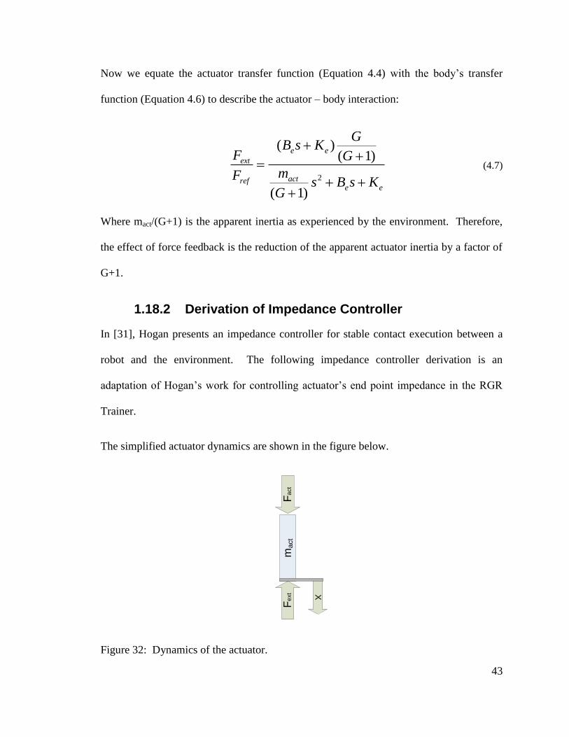
43
Now we equate the actuator transfer function (Equation 4.4) with the body’s transfer
function (Equation 4.6) to describe the actuator – body interaction:
2
( )( 1)
( 1)
e e
ext
actrefe e
GB s K
F G
mFs B s K
G
(4.7)
Where mact/(G+1) is the apparent inertia as experienced by the environment. Therefore,
the effect of force feedback is the reduction of the apparent actuator inertia by a factor of
G+1.
1.18.2 Derivation of Impedance Controller
In [31], Hogan presents an impedance controller for stable contact execution between a
robot and the environment. The following impedance controller derivation is an
adaptation of Hogan’s work for controlling actuator’s end point impedance in the RGR
Trainer.
The simplified actuator dynamics are shown in the figure below.
Fa
ct
Fe
xt
ma
ct
X
Figure 32: Dynamics of the actuator.
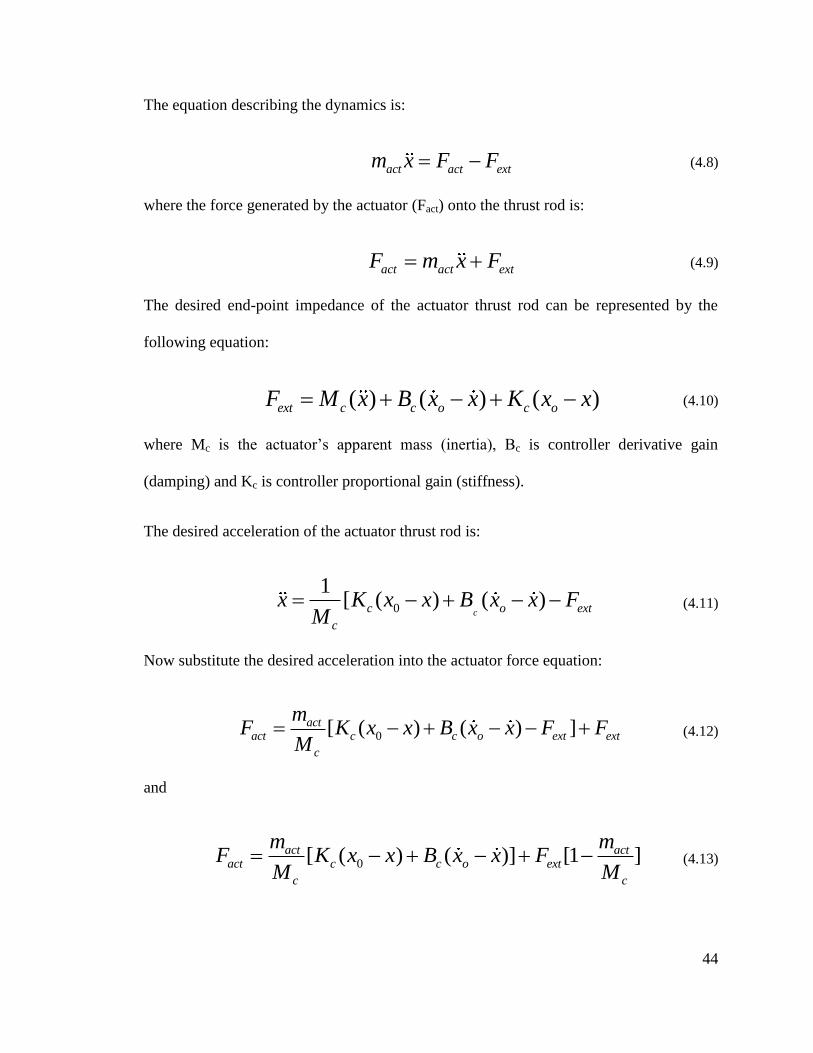
44
The equation describing the dynamics is:
act act extm x F F (4.8)
where the force generated by the actuator (Fact) onto the thrust rod is:
act act extF m x F (4.9)
The desired end-point impedance of the actuator thrust rod can be represented by the
following equation:
( ) ( ) ( )ext c c o c oF M x B x x K x x (4.10)
where Mc is the actuator’s apparent mass (inertia), Bc is controller derivative gain
(damping) and Kc is controller proportional gain (stiffness).
The desired acceleration of the actuator thrust rod is:
0
1[ ( ) ( )
cc o ext
c
x K x x B x x FM
(4.11)
Now substitute the desired acceleration into the actuator force equation:
0[ ( ) ( ) ]actact c c o ext ext
c
mF K x x B x x F F
M
(4.12)
and
0[ ( ) ( )] [1 ]act actact c c o ext
c c
m mF K x x B x x F
M M
(4.13)
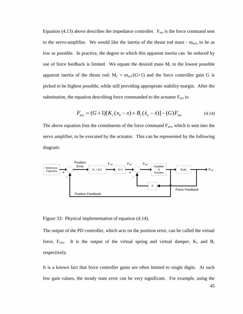
45
Equation (4.13) above describes the impedance controller. Fact is the force command sent
to the servo-amplifier. We would like the inertia of the thrust rod mass - mact, to be as
low as possible. In practice, the degree to which this apparent inertia can be reduced by
use of force feedback is limited. We equate the desired mass Mc to the lowest possible
apparent inertia of the thrust rod: Mc = mact/(G+1) and the force controller gain G is
picked to be highest possible, while still providing appropriate stability margin. After the
substitution, the equation describing force commanded to the actuator Fact is:
0( 1)[ ( ) ( )] ( )act c c o extF G K x x B x x G F (4.14)
The above equation lists the constituents of the force command Fact, which is sent into the
servo amplifier, to be executed by the actuator. This can be represented by the following
diagram:
Reference
Trajectory
Amplifier
&
Actuator
Kc + Bcs
Position Feedback
Position
ErrorFvirt
+-
+-
Force Feedback
Body FextG+1
G
FactFref
Figure 33: Physical implementation of equation (4.14).
The output of the PD controller, which acts on the position error, can be called the virtual
force, Fvirt. It is the output of the virtual spring and virtual damper, Kc and Bc
respectively.
It is a known fact that force controller gains are often limited to single digits. At such
low gain values, the steady state error can be very significant. For example, using the
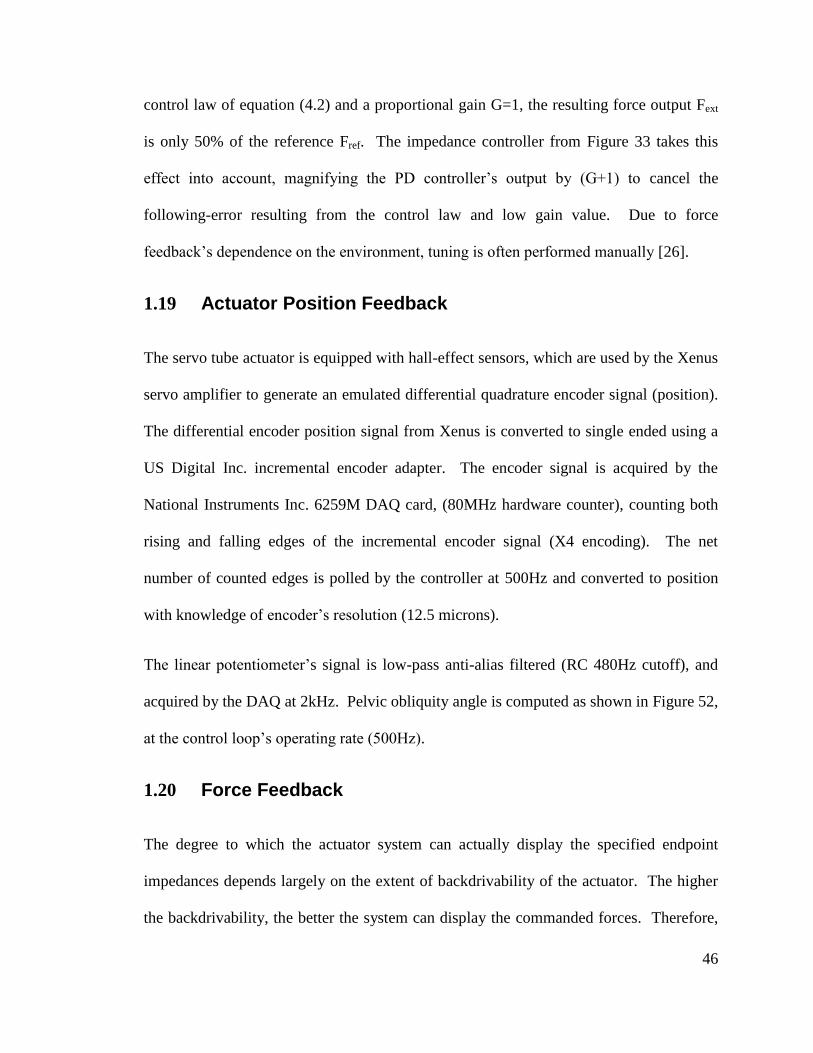
46
control law of equation (4.2) and a proportional gain G=1, the resulting force output Fext
is only 50% of the reference Fref. The impedance controller from Figure 33 takes this
effect into account, magnifying the PD controller’s output by (G+1) to cancel the
following-error resulting from the control law and low gain value. Due to force
feedback’s dependence on the environment, tuning is often performed manually [26].
1.19 Actuator Position Feedback
The servo tube actuator is equipped with hall-effect sensors, which are used by the Xenus
servo amplifier to generate an emulated differential quadrature encoder signal (position).
The differential encoder position signal from Xenus is converted to single ended using a
US Digital Inc. incremental encoder adapter. The encoder signal is acquired by the
National Instruments Inc. 6259M DAQ card, (80MHz hardware counter), counting both
rising and falling edges of the incremental encoder signal (X4 encoding). The net
number of counted edges is polled by the controller at 500Hz and converted to position
with knowledge of encoder’s resolution (12.5 microns).
The linear potentiometer’s signal is low-pass anti-alias filtered (RC 480Hz cutoff), and
acquired by the DAQ at 2kHz. Pelvic obliquity angle is computed as shown in Figure 52,
at the control loop’s operating rate (500Hz).
1.20 Force Feedback
The degree to which the actuator system can actually display the specified endpoint
impedances depends largely on the extent of backdrivability of the actuator. The higher
the backdrivability, the better the system can display the commanded forces. Therefore,
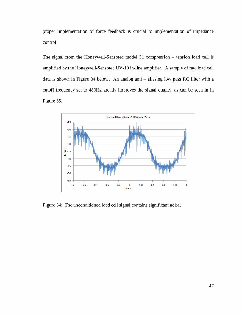
47
proper implementation of force feedback is crucial to implementation of impedance
control.
The signal from the Honeywell-Sensotec model 31 compression – tension load cell is
amplified by the Honeywell-Sensotec UV-10 in-line amplifier. A sample of raw load cell
data is shown in Figure 34 below. An analog anti – aliasing low pass RC filter with a
cutoff frequency set to 480Hz greatly improves the signal quality, as can be seen in in
Figure 35.
Figure 34: The unconditioned load cell signal contains significant noise.
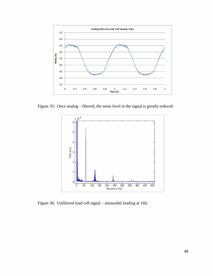
48
Figure 35: Once analog – filtered, the noise level in the signal is greatly reduced.
Figure 36: Unfiltered load cell signal – sinusoidal loading at 1Hz.
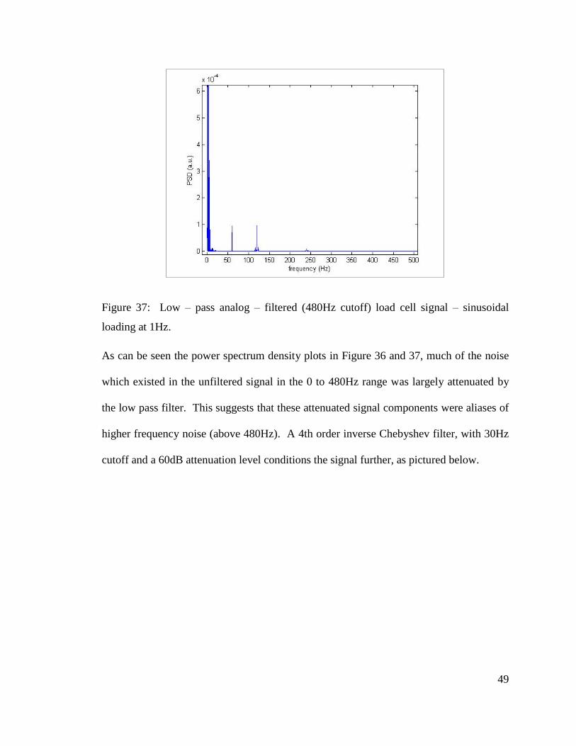
49
Figure 37: Low – pass analog – filtered (480Hz cutoff) load cell signal – sinusoidal
loading at 1Hz.
As can be seen the power spectrum density plots in Figure 36 and 37, much of the noise
which existed in the unfiltered signal in the 0 to 480Hz range was largely attenuated by
the low pass filter. This suggests that these attenuated signal components were aliases of
higher frequency noise (above 480Hz). A 4th order inverse Chebyshev filter, with 30Hz
cutoff and a 60dB attenuation level conditions the signal further, as pictured below.

50
Figure 38: Combination of analog – filtering to remove high frequency aliases, and
digital filtering produces a clean force signal.
1.21 Control Hardware and Software
The control hardware consists of a 6259M PCI data acquisition card (DAQ) from
National Instruments (Austin, TX, USA), which runs in LabVIEW Real-time operating
system (RTOS) on a dedicated PC (target) and a 4-core CPU. A host computer (laptop)
serves as the user interface. The servo tube linear actuator requires the Xenus servo
amplifier for operation. This digital amplifier can be programmed to operate in three
different modes: position, velocity or force.
51
Figure 39: Xenus servo amplifier from Copley Controls Inc.
In the force – mode, the Xenus servo – amplifier does not use a direct measure of force,
but it does however monitor the current consumed by the actuator, and a proportional –
integral (PI) controller adjusts the voltage sent to the actuator in order to coax the
requested current draw. The block diagram of the amplifier’s internal control loop is
pictured below. An automatic tuning procedure performed by the Xenus servo amplifier
set the current loop gains to Cp = 454 and Ci = 88.
Figure 40: Outline of the inner current loop contained in the Xenus servo amplifier.
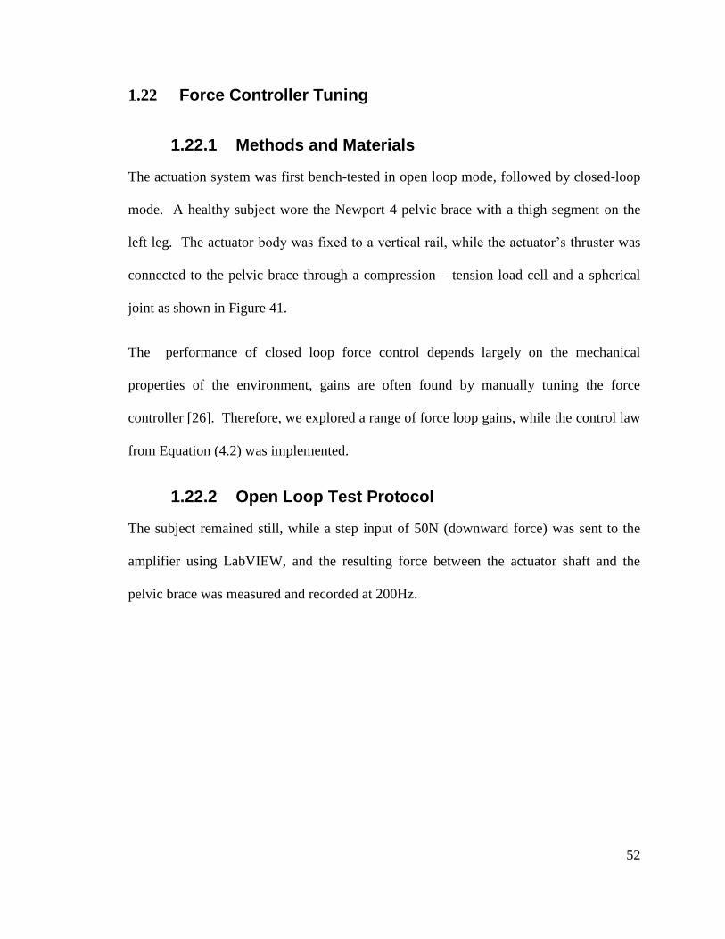
52
1.22 Force Controller Tuning
1.22.1 Methods and Materials
The actuation system was first bench-tested in open loop mode, followed by closed-loop
mode. A healthy subject wore the Newport 4 pelvic brace with a thigh segment on the
left leg. The actuator body was fixed to a vertical rail, while the actuator’s thruster was
connected to the pelvic brace through a compression – tension load cell and a spherical
joint as shown in Figure 41.
The performance of closed loop force control depends largely on the mechanical
properties of the environment, gains are often found by manually tuning the force
controller [26]. Therefore, we explored a range of force loop gains, while the control law
from Equation (4.2) was implemented.
1.22.2 Open Loop Test Protocol
The subject remained still, while a step input of 50N (downward force) was sent to the
amplifier using LabVIEW, and the resulting force between the actuator shaft and the
pelvic brace was measured and recorded at 200Hz.
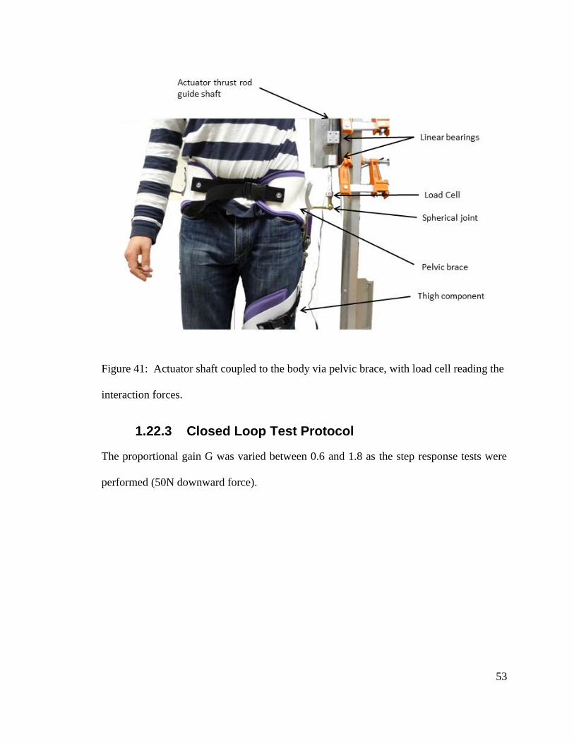
53
Figure 41: Actuator shaft coupled to the body via pelvic brace, with load cell reading the
interaction forces.
1.22.3 Closed Loop Test Protocol
The proportional gain G was varied between 0.6 and 1.8 as the step response tests were
performed (50N downward force).
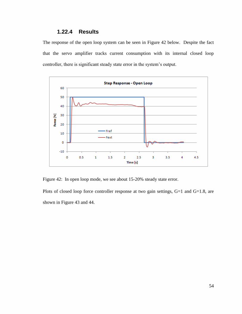
54
1.22.4 Results
The response of the open loop system can be seen in Figure 42 below. Despite the fact
that the servo amplifier tracks current consumption with its internal closed loop
controller, there is significant steady state error in the system’s output.
Figure 42: In open loop mode, we see about 15-20% steady state error.
Plots of closed loop force controller response at two gain settings, G=1 and G=1.8, are
shown in Figure 43 and 44.
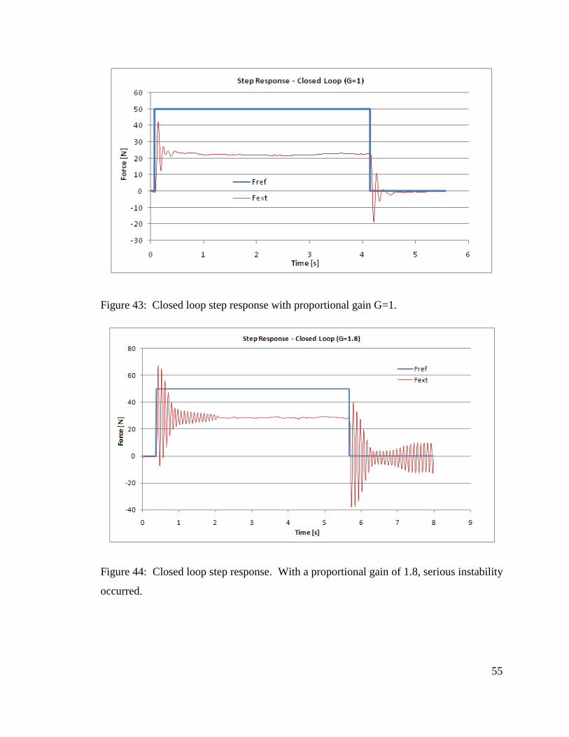
55
Figure 43: Closed loop step response with proportional gain G=1.
Figure 44: Closed loop step response. With a proportional gain of 1.8, serious instability
occurred.
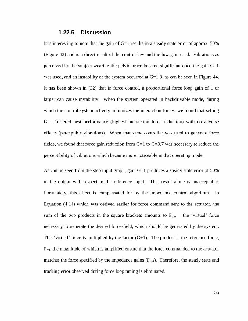
56
1.22.5 Discussion
It is interesting to note that the gain of G=1 results in a steady state error of approx. 50%
(Figure 43) and is a direct result of the control law and the low gain used. Vibrations as
perceived by the subject wearing the pelvic brace became significant once the gain G=1
was used, and an instability of the system occurred at G=1.8, as can be seen in Figure 44.
It has been shown in [32] that in force control, a proportional force loop gain of 1 or
larger can cause instability. When the system operated in backdrivable mode, during
which the control system actively minimizes the interaction forces, we found that setting
G = 1offered best performance (highest interaction force reduction) with no adverse
effects (perceptible vibrations). When that same controller was used to generate force
fields, we found that force gain reduction from G=1 to G=0.7 was necessary to reduce the
perceptibility of vibrations which became more noticeable in that operating mode.
As can be seen from the step input graph, gain G=1 produces a steady state error of 50%
in the output with respect to the reference input. That result alone is unacceptable.
Fortunately, this effect is compensated for by the impedance control algorithm. In
Equation (4.14) which was derived earlier for force command sent to the actuator, the
sum of the two products in the square brackets amounts to Fvirt – the ‘virtual’ force
necessary to generate the desired force-field, which should be generated by the system.
This ‘virtual’ force is multiplied by the factor (G+1). The product is the reference force,
Fref, the magnitude of which is amplified ensure that the force commanded to the actuator
matches the force specified by the impedance gains (Fvirt). Therefore, the steady state and
tracking error observed during force loop tuning is eliminated.
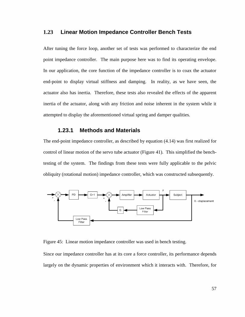
57
1.23 Linear Motion Impedance Controller Bench Tests
After tuning the force loop, another set of tests was performed to characterize the end
point impedance controller. The main purpose here was to find its operating envelope.
In our application, the core function of the impedance controller is to coax the actuator
end-point to display virtual stiffness and damping. In reality, as we have seen, the
actuator also has inertia. Therefore, these tests also revealed the effects of the apparent
inertia of the actuator, along with any friction and noise inherent in the system while it
attempted to display the aforementioned virtual spring and damper qualities.
1.23.1 Methods and Materials
The end-point impedance controller, as described by equation (4.14) was first realized for
control of linear motion of the servo tube actuator (Figure 41). This simplified the bench-
testing of the system. The findings from these tests were fully applicable to the pelvic
obliquity (rotational motion) impedance controller, which was constructed subsequently.
Figure 45: Linear motion impedance controller was used in bench testing.
Since our impedance controller has at its core a force controller, its performance depends
largely on the dynamic properties of environment which it interacts with. Therefore, for
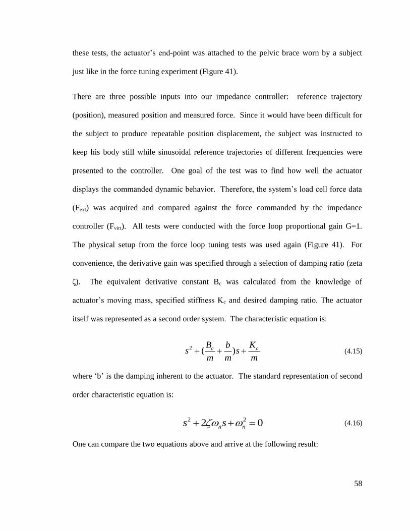
58
these tests, the actuator’s end-point was attached to the pelvic brace worn by a subject
just like in the force tuning experiment (Figure 41).
There are three possible inputs into our impedance controller: reference trajectory
(position), measured position and measured force. Since it would have been difficult for
the subject to produce repeatable position displacement, the subject was instructed to
keep his body still while sinusoidal reference trajectories of different frequencies were
presented to the controller. One goal of the test was to find how well the actuator
displays the commanded dynamic behavior. Therefore, the system’s load cell force data
(Fext) was acquired and compared against the force commanded by the impedance
controller (Fvirt). All tests were conducted with the force loop proportional gain G=1.
The physical setup from the force loop tuning tests was used again (Figure 41). For
convenience, the derivative gain was specified through a selection of damping ratio (zeta
ζ). The equivalent derivative constant Bc was calculated from the knowledge of
actuator’s moving mass, specified stiffness Kc and desired damping ratio. The actuator
itself was represented as a second order system. The characteristic equation is:
2 ( )c cB Kbs s
m m m (4.15)
where ‘b’ is the damping inherent to the actuator. The standard representation of second
order characteristic equation is:
2 22 0n ns s (4.16)
One can compare the two equations above and arrive at the following result:
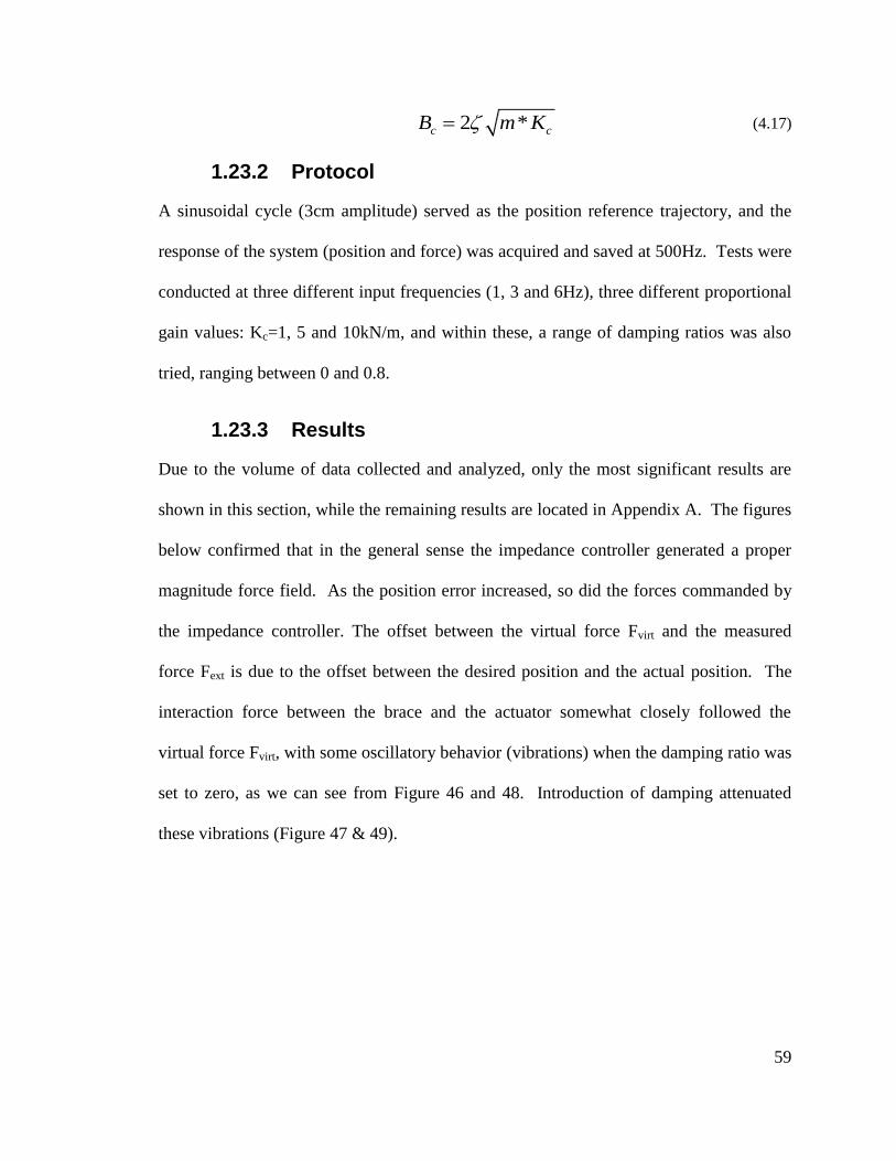
59
2 *c cB m K (4.17)
1.23.2 Protocol
A sinusoidal cycle (3cm amplitude) served as the position reference trajectory, and the
response of the system (position and force) was acquired and saved at 500Hz. Tests were
conducted at three different input frequencies (1, 3 and 6Hz), three different proportional
gain values: Kc=1, 5 and 10kN/m, and within these, a range of damping ratios was also
tried, ranging between 0 and 0.8.
1.23.3 Results
Due to the volume of data collected and analyzed, only the most significant results are
shown in this section, while the remaining results are located in Appendix A. The figures
below confirmed that in the general sense the impedance controller generated a proper
magnitude force field. As the position error increased, so did the forces commanded by
the impedance controller. The offset between the virtual force Fvirt and the measured
force Fext is due to the offset between the desired position and the actual position. The
interaction force between the brace and the actuator somewhat closely followed the
virtual force Fvirt, with some oscillatory behavior (vibrations) when the damping ratio was
set to zero, as we can see from Figure 46 and 48. Introduction of damping attenuated
these vibrations (Figure 47 & 49).
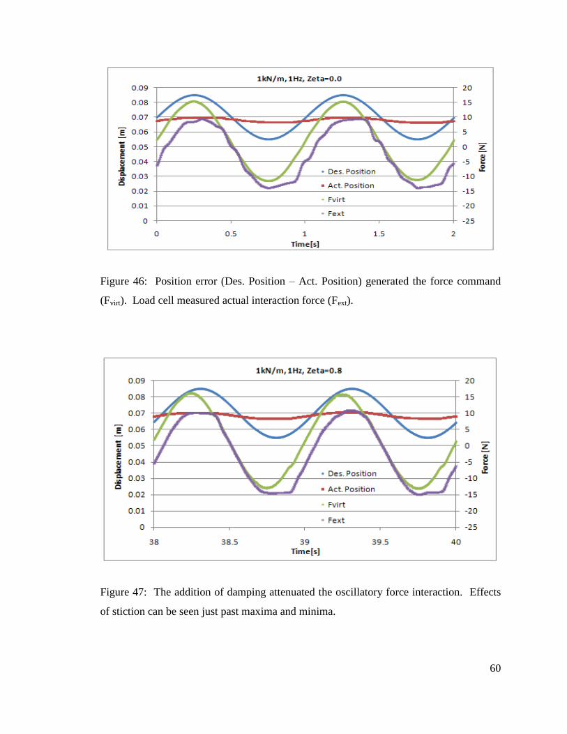
60
Figure 46: Position error (Des. Position – Act. Position) generated the force command
(Fvirt). Load cell measured actual interaction force (Fext).
Figure 47: The addition of damping attenuated the oscillatory force interaction. Effects
of stiction can be seen just past maxima and minima.
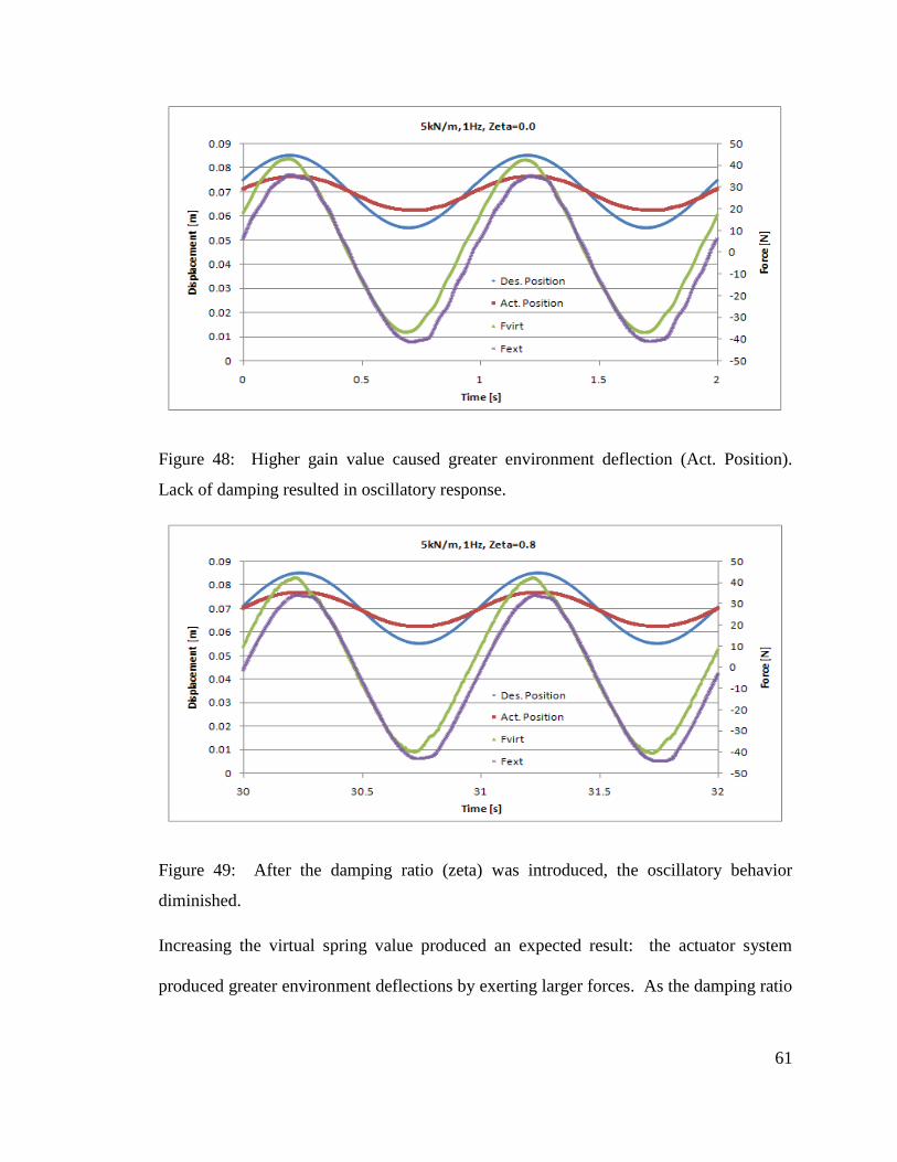
61
Figure 48: Higher gain value caused greater environment deflection (Act. Position).
Lack of damping resulted in oscillatory response.
Figure 49: After the damping ratio (zeta) was introduced, the oscillatory behavior
diminished.
Increasing the virtual spring value produced an expected result: the actuator system
produced greater environment deflections by exerting larger forces. As the damping ratio
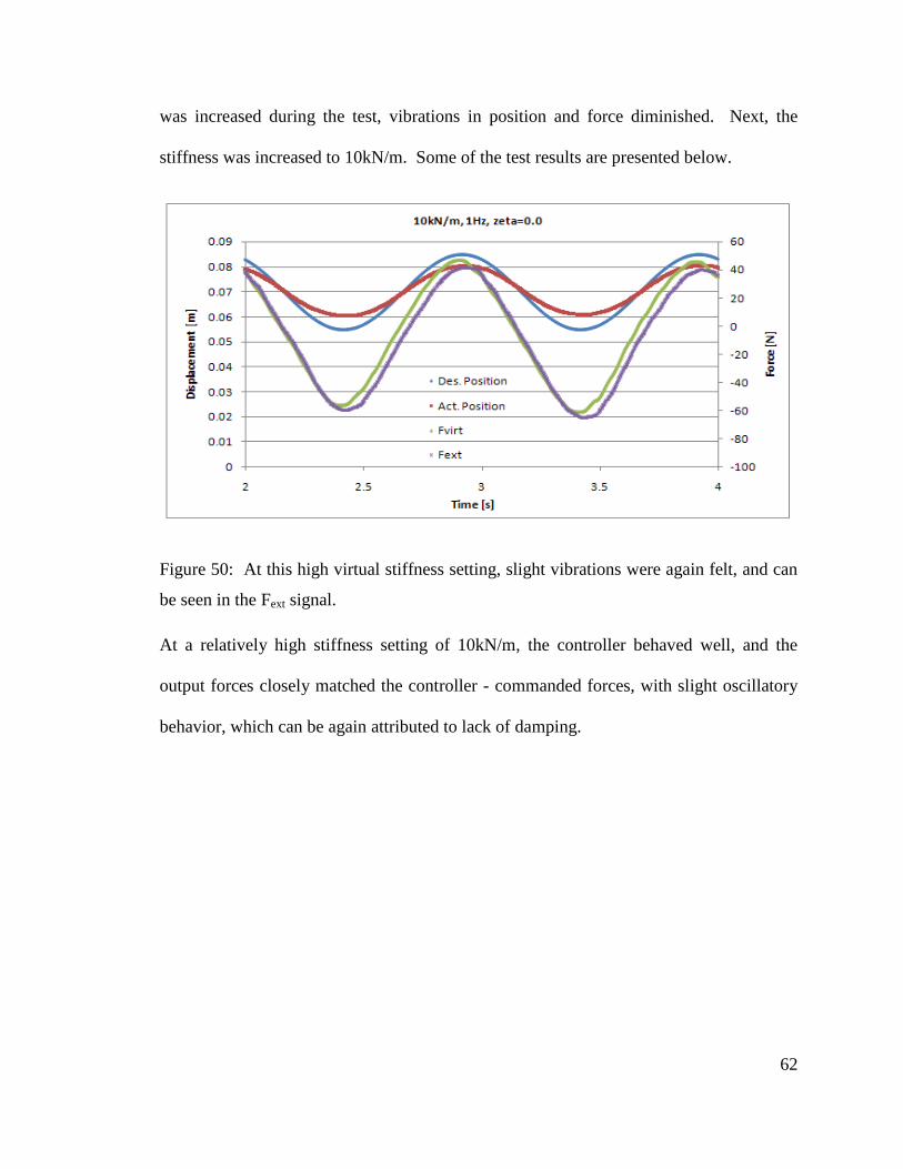
62
was increased during the test, vibrations in position and force diminished. Next, the
stiffness was increased to 10kN/m. Some of the test results are presented below.
Figure 50: At this high virtual stiffness setting, slight vibrations were again felt, and can
be seen in the Fext signal.
At a relatively high stiffness setting of 10kN/m, the controller behaved well, and the
output forces closely matched the controller - commanded forces, with slight oscillatory
behavior, which can be again attributed to lack of damping.
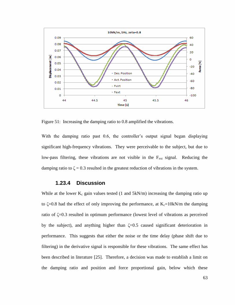
63
Figure 51: Increasing the damping ratio to 0.8 amplified the vibrations.
With the damping ratio past 0.6, the controller’s output signal began displaying
significant high-frequency vibrations. They were perceivable to the subject, but due to
low-pass filtering, these vibrations are not visible in the Fext signal. Reducing the
damping ratio to ζ = 0.3 resulted in the greatest reduction of vibrations in the system.
1.23.4 Discussion
While at the lower Kc gain values tested (1 and 5kN/m) increasing the damping ratio up
to ζ=0.8 had the effect of only improving the performance, at Kc=10kN/m the damping
ratio of ζ=0.3 resulted in optimum performance (lowest level of vibrations as perceived
by the subject), and anything higher than ζ=0.5 caused significant deterioration in
performance. This suggests that either the noise or the time delay (phase shift due to
filtering) in the derivative signal is responsible for these vibrations. The same effect has
been described in literature [25]. Therefore, a decision was made to establish a limit on
the damping ratio and position and force proportional gain, below which these
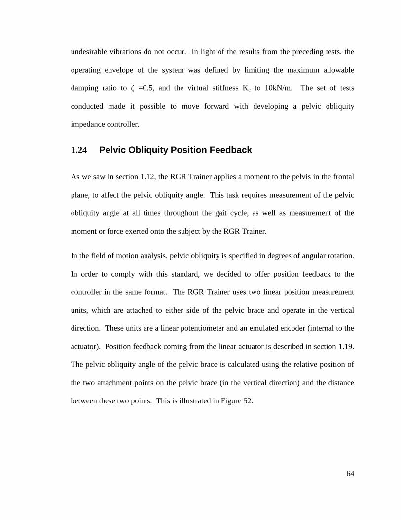
64
undesirable vibrations do not occur. In light of the results from the preceding tests, the
operating envelope of the system was defined by limiting the maximum allowable
damping ratio to ζ =0.5, and the virtual stiffness Kc to 10kN/m. The set of tests
conducted made it possible to move forward with developing a pelvic obliquity
impedance controller.
1.24 Pelvic Obliquity Position Feedback
As we saw in section 1.12, the RGR Trainer applies a moment to the pelvis in the frontal
plane, to affect the pelvic obliquity angle. This task requires measurement of the pelvic
obliquity angle at all times throughout the gait cycle, as well as measurement of the
moment or force exerted onto the subject by the RGR Trainer.
In the field of motion analysis, pelvic obliquity is specified in degrees of angular rotation.
In order to comply with this standard, we decided to offer position feedback to the
controller in the same format. The RGR Trainer uses two linear position measurement
units, which are attached to either side of the pelvic brace and operate in the vertical
direction. These units are a linear potentiometer and an emulated encoder (internal to the
actuator). Position feedback coming from the linear actuator is described in section 1.19.
The pelvic obliquity angle of the pelvic brace is calculated using the relative position of
the two attachment points on the pelvic brace (in the vertical direction) and the distance
between these two points. This is illustrated in Figure 52.
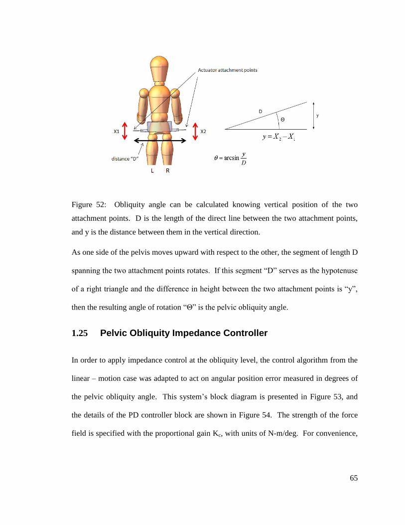
65
Figure 52: Obliquity angle can be calculated knowing vertical position of the two
attachment points. D is the length of the direct line between the two attachment points,
and y is the distance between them in the vertical direction.
As one side of the pelvis moves upward with respect to the other, the segment of length D
spanning the two attachment points rotates. If this segment “D” serves as the hypotenuse
of a right triangle and the difference in height between the two attachment points is “y”,
then the resulting angle of rotation “Θ” is the pelvic obliquity angle.
1.25 Pelvic Obliquity Impedance Controller
In order to apply impedance control at the obliquity level, the control algorithm from the
linear – motion case was adapted to act on angular position error measured in degrees of
the pelvic obliquity angle. This system’s block diagram is presented in Figure 53, and
the details of the PD controller block are shown in Figure 54. The strength of the force
field is specified with the proportional gain Kc, with units of N-m/deg. For convenience,
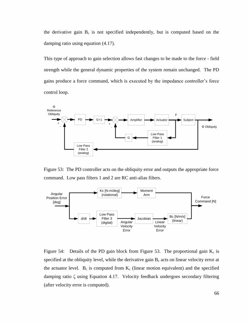
66
the derivative gain Bc is not specified independently, but is computed based on the
damping ratio using equation (4.17).
This type of approach to gain selection allows fast changes to be made to the force - field
strength while the general dynamic properties of the system remain unchanged. The PD
gains produce a force command, which is executed by the impedance controller’s force
control loop.
SubjectActuatorAmplifier
G
Low Pass
Filter 1
(analog)
PD G+1
F
-+
-+
Low Pass
Filter 2
(analog)
Θ Obliquity
Θ
Reference
Obliquity
Figure 53: The PD controller acts on the obliquity error and outputs the appropriate force
command. Low pass filters 1 and 2 are RC anti-alias filters.
d/dt
Angular
Position Error
[deg]
Angular
Velocity
Error
JacobianBc [N/m/s]
(linear)
Kc [N-m/deg]
(rotational)
Moment
ArmForce
Command [N]
Linear
Velocity
Error
Low Pass
Filter 3
(digital)
Figure 54: Details of the PD gain block from Figure 53. The proportional gain Kc is
specified at the obliquity level, while the derivative gain Bc acts on linear velocity error at
the actuator level. Bc is computed from Kc (linear motion equivalent) and the specified
damping ratio ζ using Equation 4.17. Velocity feedback undergoes secondary filtering
(after velocity error is computed).
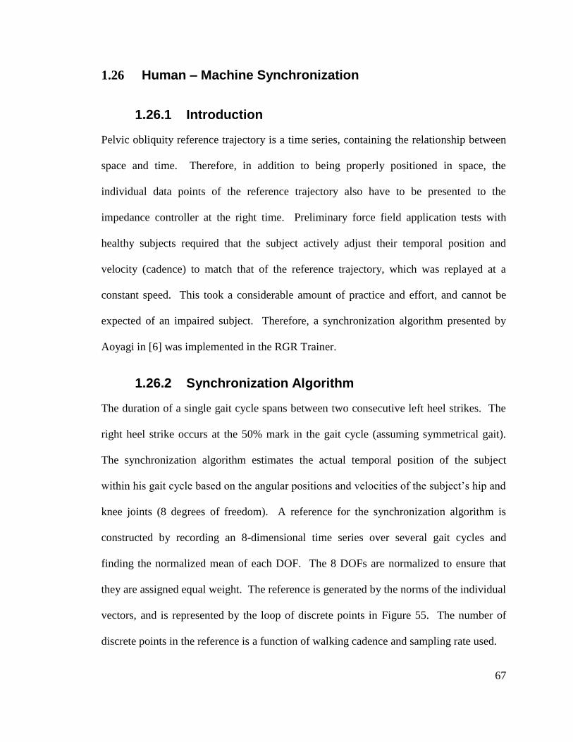
67
1.26 Human – Machine Synchronization
1.26.1 Introduction
Pelvic obliquity reference trajectory is a time series, containing the relationship between
space and time. Therefore, in addition to being properly positioned in space, the
individual data points of the reference trajectory also have to be presented to the
impedance controller at the right time. Preliminary force field application tests with
healthy subjects required that the subject actively adjust their temporal position and
velocity (cadence) to match that of the reference trajectory, which was replayed at a
constant speed. This took a considerable amount of practice and effort, and cannot be
expected of an impaired subject. Therefore, a synchronization algorithm presented by
Aoyagi in [6] was implemented in the RGR Trainer.
1.26.2 Synchronization Algorithm
The duration of a single gait cycle spans between two consecutive left heel strikes. The
right heel strike occurs at the 50% mark in the gait cycle (assuming symmetrical gait).
The synchronization algorithm estimates the actual temporal position of the subject
within his gait cycle based on the angular positions and velocities of the subject’s hip and
knee joints (8 degrees of freedom). A reference for the synchronization algorithm is
constructed by recording an 8-dimensional time series over several gait cycles and
finding the normalized mean of each DOF. The 8 DOFs are normalized to ensure that
they are assigned equal weight. The reference is generated by the norms of the individual
vectors, and is represented by the loop of discrete points in Figure 55. The number of
discrete points in the reference is a function of walking cadence and sampling rate used.
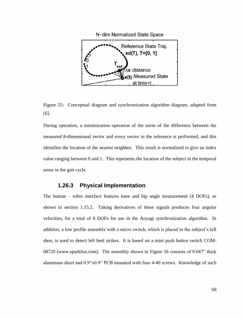
68
Figure 55: Conceptual diagram and synchronization algorithm diagram, adapted from
[6].
During operation, a minimization operation of the norm of the difference between the
measured 8-dimensional vector and every vector in the reference is performed, and this
identifies the location of the nearest neighbor. This result is normalized to give an index
value ranging between 0 and 1. This represents the location of the subject in the temporal
sense in the gait cycle.
1.26.3 Physical Implementation
The human – robot interface features knee and hip angle measurement (4 DOFs), as
shown in section 1.15.2. Taking derivatives of these signals produces four angular
velocities, for a total of 8 DOFs for use in the Aoyagi synchronization algorithm. In
addition, a low profile assembly with a micro switch, which is placed in the subject’s left
shoe, is used to detect left heel strikes. It is based on a mini push button switch COM-
08720 (www.sparkfun.com). The assembly shown in Figure 56 consists of 0.047” thick
aluminum sheet and 0.9”x0.9” PCB mounted with four 4-40 screws. Knowledge of such
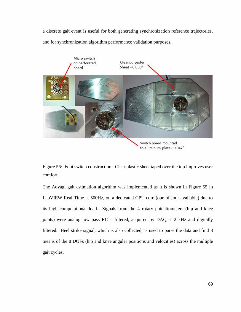
69
a discrete gait event is useful for both generating synchronization reference trajectories,
and for synchronization algorithm performance validation purposes.
Figure 56: Foot switch construction. Clear plastic sheet taped over the top improves user
comfort.
The Aoyagi gait estimation algorithm was implemented as it is shown in Figure 55 in
LabVIEW Real Time at 500Hz, on a dedicated CPU core (one of four available) due to
its high computational load. Signals from the 4 rotary potentiometers (hip and knee
joints) were analog low pass RC – filtered, acquired by DAQ at 2 kHz and digitally
filtered. Heel strike signal, which is also collected, is used to parse the data and find 8
means of the 8 DOFs (hip and knee angular positions and velocities) across the multiple
gait cycles.
70
1.26.4 Quantitative Evaluation of Performance
One way to quantify the synchronization algorithm’s performance is to compare its
output to a nominal metric. While walking at constant speed and cadence with
symmetric gait, a healthy subject’s progression through his gait cycle generates a straight
line, when plotted against time. We can create a useful metric by generating a linear
interpolation between a cyclic discrete gait cycle event, such as left heel strike. This
allows us quantify the performance of the synchronization algorithm. Therefore, a
“nominal” time series was created by concatenating vectors generated by linear
interpolation between the consecutive heel strikes in a sample dataset.
Figure 57: MATLAB’s “unwrap” function produces continuous curves of periodic time
series. The range of phase angle of 5 radians to 75 radians covers approx. 11 full gait
cycles.
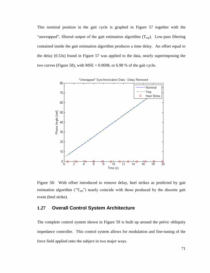
71
This nominal position in the gait cycle is graphed in Figure 57 together with the
“unwrapped”, filtered output of the gait estimation algorithm (Trep). Low-pass filtering
contained inside the gait estimation algorithm produces a time delay. An offset equal to
the delay (0.53s) found in Figure 57 was applied to the data, nearly superimposing the
two curves (Figure 58), with MSE = 0.0698, or 6.98 % of the gait cycle.
Figure 58: With offset introduced to remove delay, heel strikes as predicted by gait
estimation algorithm (“Trep”) nearly coincide with those produced by the discrete gait
event (heel strike).
1.27 Overall Control System Architecture
The complete control system shown in Figure 59 is built up around the pelvic obliquity
impedance controller. This control system allows for modulation and fine-tuning of the
force field applied onto the subject in two major ways.
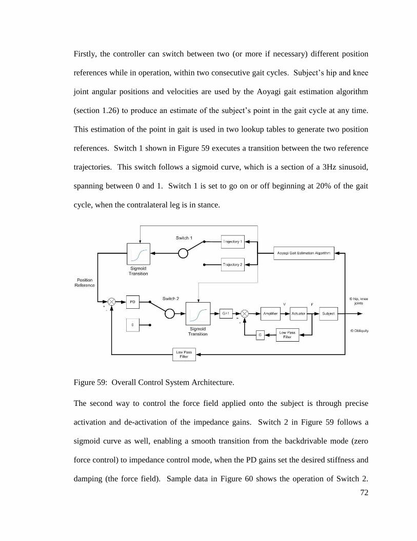
72
Firstly, the controller can switch between two (or more if necessary) different position
references while in operation, within two consecutive gait cycles. Subject’s hip and knee
joint angular positions and velocities are used by the Aoyagi gait estimation algorithm
(section 1.26) to produce an estimate of the subject’s point in the gait cycle at any time.
This estimation of the point in gait is used in two lookup tables to generate two position
references. Switch 1 shown in Figure 59 executes a transition between the two reference
trajectories. This switch follows a sigmoid curve, which is a section of a 3Hz sinusoid,
spanning between 0 and 1. Switch 1 is set to go on or off beginning at 20% of the gait
cycle, when the contralateral leg is in stance.
Figure 59: Overall Control System Architecture.
The second way to control the force field applied onto the subject is through precise
activation and de-activation of the impedance gains. Switch 2 in Figure 59 follows a
sigmoid curve as well, enabling a smooth transition from the backdrivable mode (zero
force control) to impedance control mode, when the PD gains set the desired stiffness and
damping (the force field). Sample data in Figure 60 shows the operation of Switch 2.
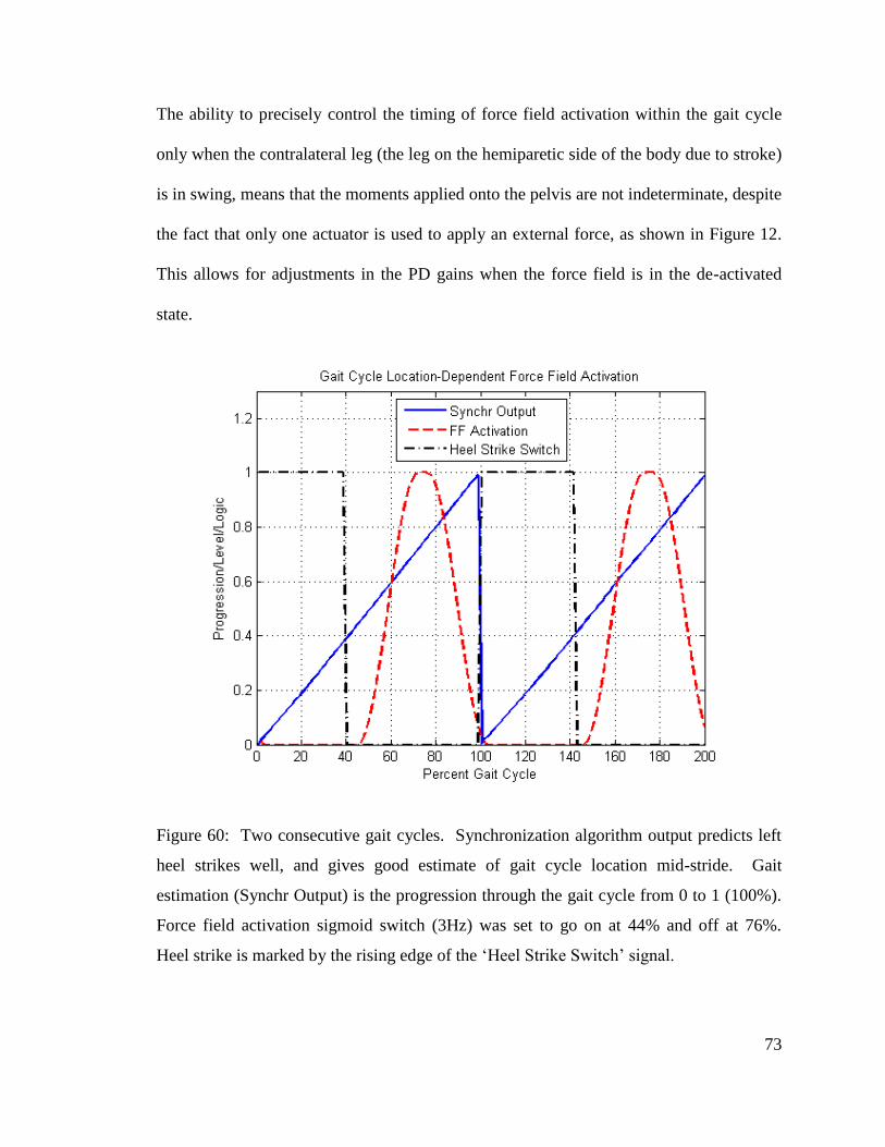
73
The ability to precisely control the timing of force field activation within the gait cycle
only when the contralateral leg (the leg on the hemiparetic side of the body due to stroke)
is in swing, means that the moments applied onto the pelvis are not indeterminate, despite
the fact that only one actuator is used to apply an external force, as shown in Figure 12.
This allows for adjustments in the PD gains when the force field is in the de-activated
state.
Figure 60: Two consecutive gait cycles. Synchronization algorithm output predicts left
heel strikes well, and gives good estimate of gait cycle location mid-stride. Gait
estimation (Synchr Output) is the progression through the gait cycle from 0 to 1 (100%).
Force field activation sigmoid switch (3Hz) was set to go on at 44% and off at 76%.
Heel strike is marked by the rising edge of the ‘Heel Strike Switch’ signal.
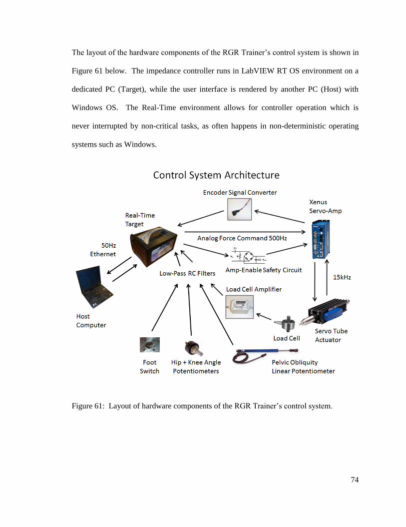
74
The layout of the hardware components of the RGR Trainer’s control system is shown in
Figure 61 below. The impedance controller runs in LabVIEW RT OS environment on a
dedicated PC (Target), while the user interface is rendered by another PC (Host) with
Windows OS. The Real-Time environment allows for controller operation which is
never interrupted by non-critical tasks, as often happens in non-deterministic operating
systems such as Windows.
Figure 61: Layout of hardware components of the RGR Trainer’s control system.
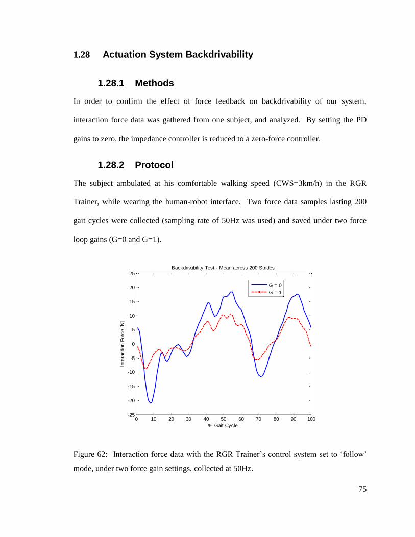
75
1.28 Actuation System Backdrivability
1.28.1 Methods
In order to confirm the effect of force feedback on backdrivability of our system,
interaction force data was gathered from one subject, and analyzed. By setting the PD
gains to zero, the impedance controller is reduced to a zero-force controller.
1.28.2 Protocol
The subject ambulated at his comfortable walking speed (CWS=3km/h) in the RGR
Trainer, while wearing the human-robot interface. Two force data samples lasting 200
gait cycles were collected (sampling rate of 50Hz was used) and saved under two force
loop gains (G=0 and G=1).
Figure 62: Interaction force data with the RGR Trainer’s control system set to ‘follow’
mode, under two force gain settings, collected at 50Hz.
0 10 20 30 40 50 60 70 80 90 100-25
-20
-15
-10
-5
0
5
10
15
20
25
% Gait Cycle
Inte
raction F
orc
e [
N]
Backdrivability Test - Mean across 200 Strides
G = 0
G = 1
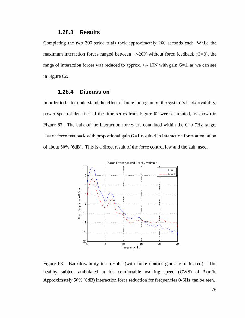
76
1.28.3 Results
Completing the two 200-stride trials took approximately 260 seconds each. While the
maximum interaction forces ranged between +/-20N without force feedback (G=0), the
range of interaction forces was reduced to approx. +/- 10N with gain G=1, as we can see
in Figure 62.
1.28.4 Discussion
In order to better understand the effect of force loop gain on the system’s backdrivability,
power spectral densities of the time series from Figure 62 were estimated, as shown in
Figure 63. The bulk of the interaction forces are contained within the 0 to 7Hz range.
Use of force feedback with proportional gain G=1 resulted in interaction force attenuation
of about 50% (6dB). This is a direct result of the force control law and the gain used.
Figure 63: Backdrivability test results (with force control gains as indicated). The
healthy subject ambulated at his comfortable walking speed (CWS) of 3km/h.
Approximately 50% (6dB) interaction force reduction for frequencies 0-6Hz can be seen.
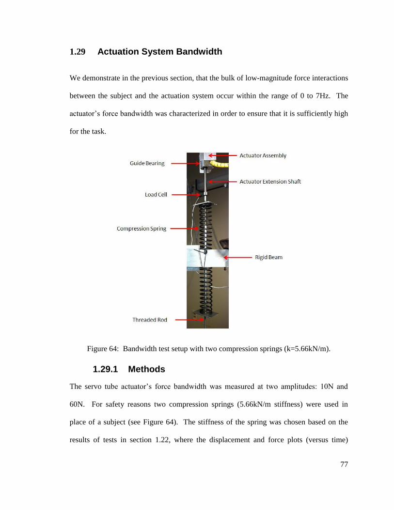
77
1.29 Actuation System Bandwidth
We demonstrate in the previous section, that the bulk of low-magnitude force interactions
between the subject and the actuation system occur within the range of 0 to 7Hz. The
actuator’s force bandwidth was characterized in order to ensure that it is sufficiently high
for the task.
Figure 64: Bandwidth test setup with two compression springs (k=5.66kN/m).
1.29.1 Methods
The servo tube actuator’s force bandwidth was measured at two amplitudes: 10N and
60N. For safety reasons two compression springs (5.66kN/m stiffness) were used in
place of a subject (see Figure 64). The stiffness of the spring was chosen based on the
results of tests in section 1.22, where the displacement and force plots (versus time)
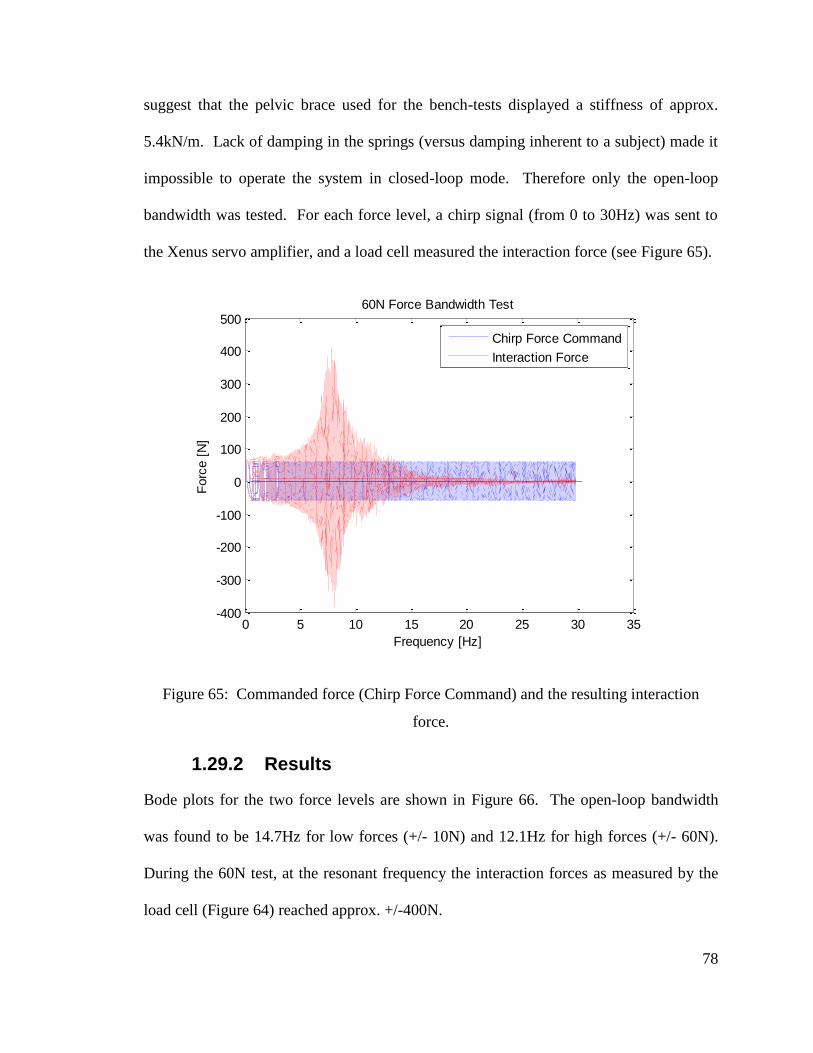
78
suggest that the pelvic brace used for the bench-tests displayed a stiffness of approx.
5.4kN/m. Lack of damping in the springs (versus damping inherent to a subject) made it
impossible to operate the system in closed-loop mode. Therefore only the open-loop
bandwidth was tested. For each force level, a chirp signal (from 0 to 30Hz) was sent to
the Xenus servo amplifier, and a load cell measured the interaction force (see Figure 65).
Figure 65: Commanded force (Chirp Force Command) and the resulting interaction
force.
1.29.2 Results
Bode plots for the two force levels are shown in Figure 66. The open-loop bandwidth
was found to be 14.7Hz for low forces (+/- 10N) and 12.1Hz for high forces (+/- 60N).
During the 60N test, at the resonant frequency the interaction forces as measured by the
load cell (Figure 64) reached approx. +/-400N.
0 5 10 15 20 25 30 35-400
-300
-200
-100
0
100
200
300
400
500
Frequency [Hz]
Forc
e [
N]
60N Force Bandwidth Test
Chirp Force Command
Interaction Force
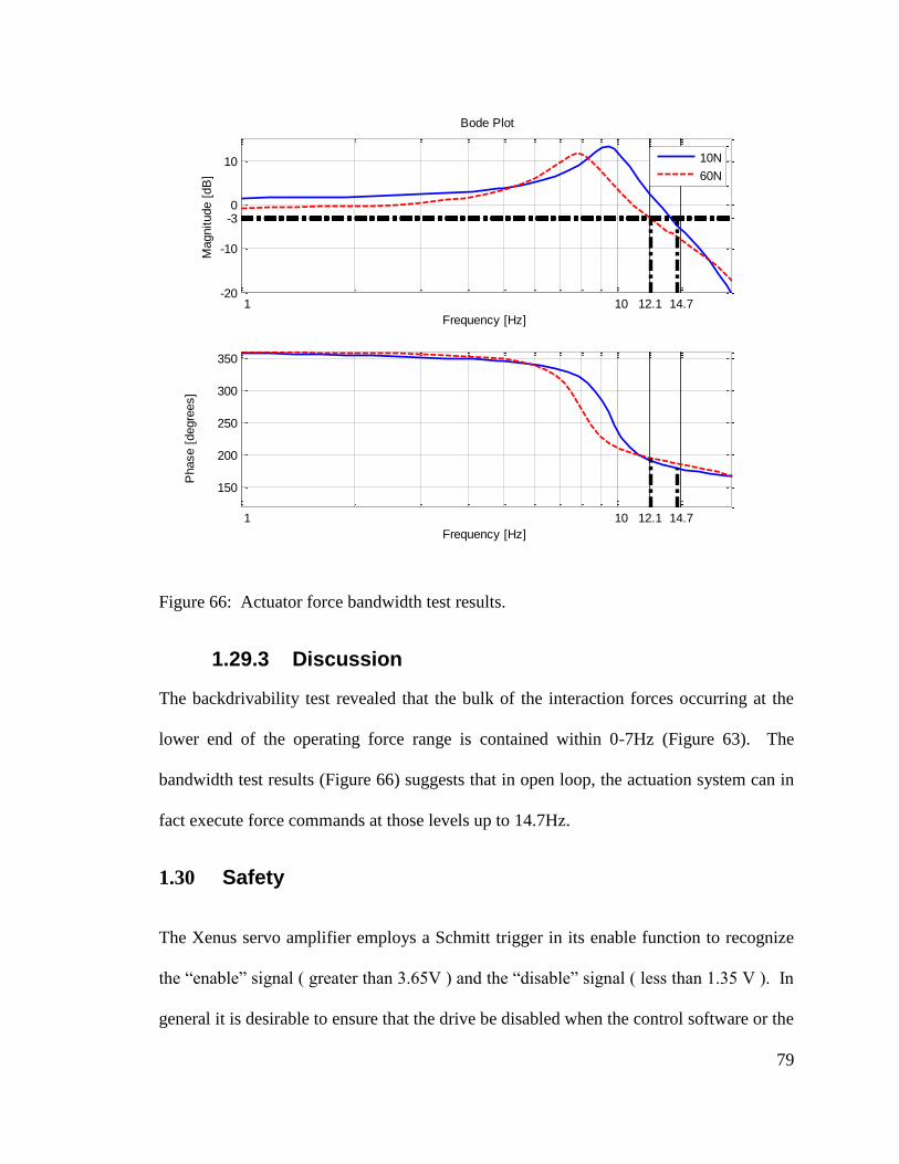
79
Figure 66: Actuator force bandwidth test results.
1.29.3 Discussion
The backdrivability test revealed that the bulk of the interaction forces occurring at the
lower end of the operating force range is contained within 0-7Hz (Figure 63). The
bandwidth test results (Figure 66) suggests that in open loop, the actuation system can in
fact execute force commands at those levels up to 14.7Hz.
1.30 Safety
The Xenus servo amplifier employs a Schmitt trigger in its enable function to recognize
the “enable” signal ( greater than 3.65V ) and the “disable” signal ( less than 1.35 V ). In
general it is desirable to ensure that the drive be disabled when the control software or the
1 10 12.1 14.7-20
-10
-3 0
10
Frequency [Hz]
Magnitude [
dB
]
10N
60N
1 10 12.1 14.7
150
200
250
300
350
Frequency [Hz]
Phase [
degre
es]
Bode Plot
80
computer itself fail. A simple solution of using a DAQ analog output channel to send an
“enable” signal while the controller is in operation, and a disable signal when it stops is
not perfectly reliable. Unfortunately, when LabVIEW software fails, the National
Instruments 6259M card continues to output the last value for as long as there is power
supplied to the computer. This creates a potentially dangerous situation, especially with a
highly back-drivable system as ours working under impedance control. For example
after a software failure, a high - force command from the time of failure will remain.
Physically unplugging the servo amplifier’s mains electrical supply would cause the
actuator to cease exerting force thus becoming easily backdriven to a new position.
Then, returning main power to the amplifier could cause a sudden, unexpected
acceleration of the thrust rod, possibly causing injury and damage to the actuator
assembly.
To address this problem, one solution is to use an external microchip with a “watchdog”
feature, which detects software failure, as was done in [20]. Our solution was to use a
simple analog circuit to provide the enable signal to the Xenus servo amplifier only when
LabVIEW is active. A dedicated DAQ output was configured to supply a sinusoidal
voltage signal of 100Hz frequency and ranging between 0V and 10V. This signal was
routed through an analog RC high-pass filter, with the cutoff frequency on the order of
several Hz to avoid excessive signal attenuation. Then, the signal was rectified with a
Gratz bridge rectifier and smoothed with help of a capacitor placed in parallel, as is
shown in Figure 67. The result was a slightly varying voltage output which successfully
enabled the Xenus servo amplifier when the input was of proper frequency and
magnitude. At the same time, the circuit’s output changed to 0V whenever the input was
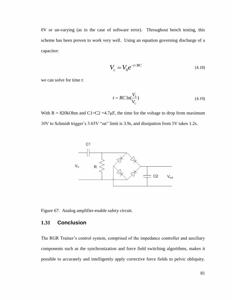
81
0V or un-varying (as in the case of software error). Throughout bench testing, this
scheme has been proven to work very well. Using an equation governing discharge of a
capacitor:
/
0
t RC
cV V e (4.18)
we can solve for time t:
0ln( )C
Vt RC
V (4.19)
With R = 820kOhm and C1=C2 =4.7μF, the time for the voltage to drop from maximum
10V to Schmidt trigger’s 3.65V “on” limit is 3.9s, and dissipation from 5V takes 1.2s.
Figure 67: Analog amplifier-enable safety circuit.
1.31 Conclusion
The RGR Trainer’s control system, comprised of the impedance controller and auxiliary
components such as the synchronization and force field switching algorithms, makes it
possible to accurately and intelligently apply corrective force fields to pelvic obliquity.

82
With just one actuator, such functionality would not have been possible without the
precise timing of force field activation. The next chapter describes the various
experiments, which we performed on healthy subjects. These experiments put the
individual subsystems of the RGR Trainer to the test, proving the RGR Trainer’s
usefulness as a device for gait retraining.

83
Healthy Subject Testing
1.32 Introduction
Gait rehabilitation techniques fall under two categories: neurophysiological or motor
learning. In the classic neurophysiological gait rehabilitation techniques, the physical
therapist (PT) supports the patient’s correct movement patterns, acting as a problem
solver and decision maker, rendering the patient a relatively passive recipient [33]. On
the other hand, motor learning techniques stress active patient involvement in context-
specific motor tasks. Robotic gait rehabilitation is intensive, repetitive and task-oriented,
and therefore aligns itself well with motor-learning techniques.
Design of optimal gait retraining therapies for patients post stroke requires thorough
understanding of normal, as well as pathological gait patterns. Human development
period provides some insight into the former. Infants exhibit stepping behavior even
before birth, thus before the motor cortex in the brain can effectively send motor
commands to the muscles involved, but their stepping pattern lacks proper ankle joint
control for ground clearance, resulting in toe-drag. Impaired dorsiflexion during the
swing phase of the gait cycle is also the most common problem in walking after injury to
motor areas of the brain [34].
Locomotion results from intricate dynamic interactions between a central program and
feedback mechanisms” [34]. The central program, contained in the spinal column’s
central pattern generators (CPGs), can generate basic locomotion patterns to steer, trigger
and stop locomotion while feedback from muscles, skin afferents, vision, hearing, and
84
sense of balance are used to dynamically adjust the locomotion pattern to the
requirements of the environment [35]. Therefore, it is the various brain regions such as
the cerebral motor cortex, cerebellum, and brain stem, which are responsible for the fine
control of the gait pattern. Recent work suggests that both peripheral sensory information
and inputs from the motor cortex reshape the function of the CPG, especially during brain
plasticity post-stroke. In fact, it is believed that the locomotor patterns generated by the
CPGs are not sufficient for over-ground walking, and supraspinal control is needed to
provide both the drive for locomotion as well as the coordination to negotiate a complex
environment [36].
Motor adaptation studies, which were first conducted by Shadmehr and Mussa-Ivaldi [37]
for upper extremities, are now being used on lower extremities, in order to better
understand the mechanisms governing locomotion. Motor adaptation “…is the
modification of a movement from trial-to-trial based on error feedback in which the
following criteria are met. First, the movement retains its identity of being a specific
action (e.g. ‘reaching’) but changes in terms of one or more parameters (e.g. the pattern
of force or direction). Second, the change occurs with repetition or practice of the
behavior and is gradual over minutes to hours. Third, once adapted, individuals cannot
retrieve the prior behavior; instead, they show ‘after-effects’ and must ‘de-adapt’ the
behavior with practice in the same gradual, continuous manner back to the original state”
[38]. The reactive or feedback-driven adaptations differ importantly from predictive
adaptations in that they occur more quickly in response to ongoing afferent feedback (i.e.,
do not require practice) and are not stored by the nervous system (i.e., do not produce
aftereffects) [39].
85
Since motor adaptation is one of the factors responsible for variability in rehabilitation
outcomes following robot-assisted gait retraining, it is hoped that subjects’ performance
in motor adaptation studies will be predictive of rehabilitation outcomes. Therefore,
currently motor adaptations in lower extremities are being studied by several teams. A
direct extension of the method first used by Shadmehr and Mussa-Ivaldi which applies
velocity-dependent perturbations perpendicular to the direction of motion was
implemented in the Lokomat by Cajigas et.al [40]. Motor adaptations were also
investigated on a number of healthy subjects in the active leg exoskeleton (ALEX) [41].
In the LOPES [42], motor adaptations were studied while the goal of the training was to
affect foot ground clearance during swing, by applying a vertical force proportional to the
horizontal velocity of the ankle. Such choice of protocol was inspired by work done on
upper limb motor adaptations, but interestingly some of the researchers’ findings
contradicted their hypotheses. Therefore, they urge caution in implementing upper limp
research principles for lower limbs.
Another team, which used split belt treadmill gait training with stroke survivors was able
to induce after-effects in gait symmetry [43]. Both this study and another one with upper
extremities have found that adapting the patient to a perturbation that worsened or
amplified their error was what drove adaptation to result in after-effects that improved
their movement [38]. The after-effects were transient, and diminished in a matter of
minutes, a process called wash-out. That’s why researchers are investigating motor
learning
Motor learning is “the formation of a new motor pattern that occurs via long-term
practice (i.e. days, weeks, years). After the new movement pattern is learnt, it is stored
86
and can be immediately brought up and used in the appropriate context (i.e. in contrast to
adaptation, no practice period is required). Individuals may store many learned motor
plans or calibrations that allow for efficient switching from one to another” [38]. The
hope is that since clinicians often work with patients who can perform certain tasks such
as walking or reaching, but their movements are slow, misdirected, inaccurate, or
inefficient, it may be possible to help them recalibrate these movements, instead of
learning completely new movement patterns.
Hip-hiking, which is an abnormal pelvic obliquity pattern, is the most common secondary
gait deviation, and while motor learning principles are being increasingly used to study
locomotion, no such studies have ever targeted the control of pelvic obliquity. This
motivated the various protocols described in this chapter, which aimed to:
- Demonstrate that the RGR Trainer can effectively guide the pelvis in the frontal
plane via force fields to alter pelvic obliquity.
- Investigate whether the RGR Trainer can induce motor adaptations in pelvic
obliquity control.
The protocols presented here constitute the most significant approaches which were
undertaken in healthy subject tests in the RGR Trainer. All subject tests were conducted
in accordance with methods approved by the Spaulding Rehabilitation Hospital’s Internal
Review Board (IRB).
87
1.33 Protocol 1
1.33.1 Hypothesis
The RGR trainer can teach the hip-hiking gait pattern to healthy adults by generating an
appropriate force field around their pelvis.
1.33.2 Protocol 1 Methods
1.33.2.1 Experimental Apparatus and Reference Trajectories
The RGR Trainer, configured to apply vertical forces on the left side of the body, was
programmed to switch between two reference trajectories: baseline and hip-hiking. The
switching action was designed to happen quickly but smoothly, occurring when left leg is
in stance (due to the small position error at that time) and following a sigmoid curve at a
frequency of 3Hz. The sigmoid is one half cycle of a 3Hz sinusoid, minimum to
maximum amplitude or vice versa, spanning between 0 and 1.
A hip-hiking pelvic obliquity reference trajectory was found in literature. A 2009 study
by Cruz et al. [44] focused on “understanding the potential causes of reduced gait speed
and compensatory frontal plane kinematics during walking in individuals post-stroke.”
The data gathered from 18 subjects post-stroke and 8 control subjects (Cruz et al.) was
used to produce curves of pelvic obliquity for both groups, as shown in Figure 68. The
mean walking speed of the patients was 1.8 km/h. Therefore, the protocol was designed
to be performed at the same walking speed. Interaction forces between the exoskeleton
worn by the subjects and the RGR Trainer’s actuation system during left leg swing were
used as the outcome measure.
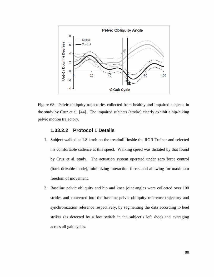
88
Figure 68: Pelvic obliquity trajectories collected from healthy and impaired subjects in
the study by Cruz et al. [44]. The impaired subjects (stroke) clearly exhibit a hip-hiking
pelvic motion trajectory.
1.33.2.2 Protocol 1 Details
1. Subject walked at 1.8 km/h on the treadmill inside the RGR Trainer and selected
his comfortable cadence at this speed. Walking speed was dictated by that found
by Cruz et al. study. The actuation system operated under zero force control
(back-drivable mode), minimizing interaction forces and allowing for maximum
freedom of movement.
2. Baseline pelvic obliquity and hip and knee joint angles were collected over 100
strides and converted into the baseline pelvic obliquity reference trajectory and
synchronization reference respectively, by segmenting the data according to heel
strikes (as detected by a foot switch in the subject’s left shoe) and averaging
across all gait cycles.
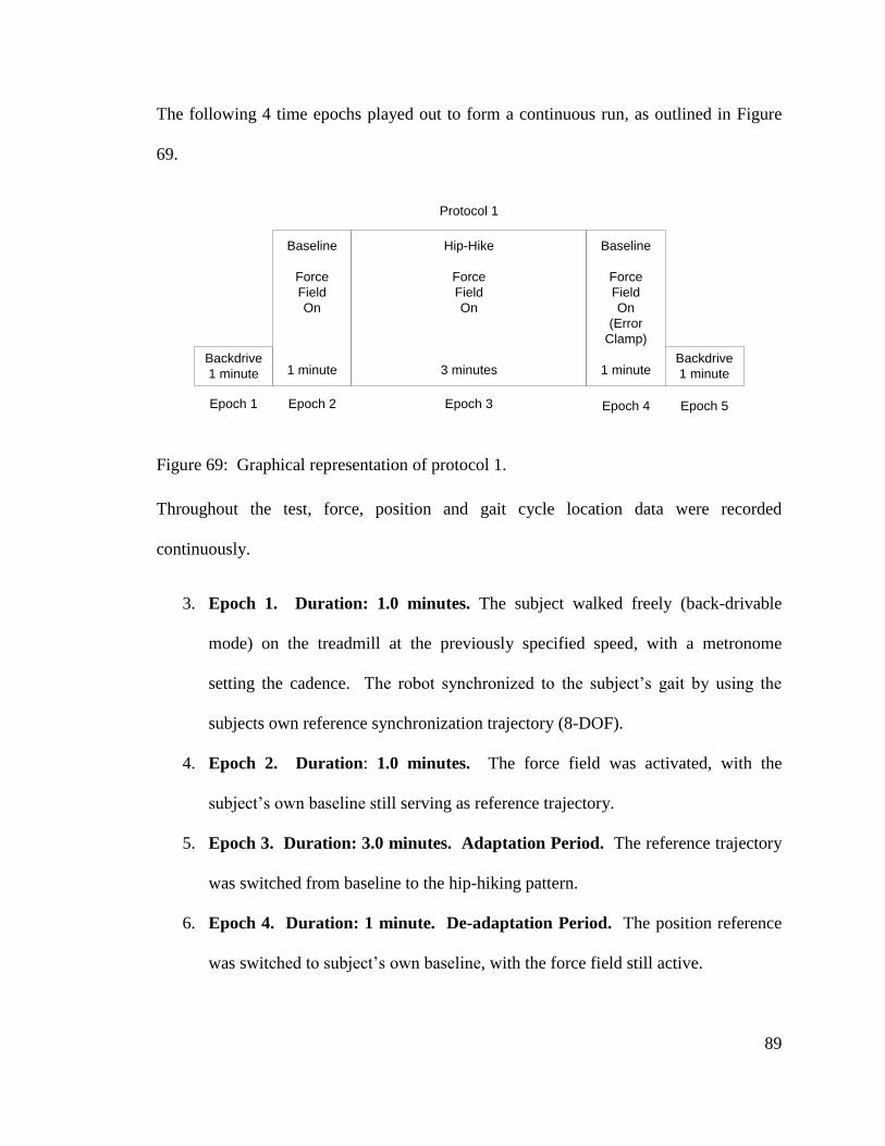
89
The following 4 time epochs played out to form a continuous run, as outlined in Figure
69.
Backdrive
1 minute
Baseline
Force
Field
On
1 minute
Hip-Hike
Force
Field
On
3 minutes
Baseline
Force
Field
On
(Error
Clamp)
1 minuteBackdrive
1 minute
Epoch 1 Epoch 2 Epoch 3 Epoch 4 Epoch 5
Protocol 1
Figure 69: Graphical representation of protocol 1.
Throughout the test, force, position and gait cycle location data were recorded
continuously.
3. Epoch 1. Duration: 1.0 minutes. The subject walked freely (back-drivable
mode) on the treadmill at the previously specified speed, with a metronome
setting the cadence. The robot synchronized to the subject’s gait by using the
subjects own reference synchronization trajectory (8-DOF).
4. Epoch 2. Duration: 1.0 minutes. The force field was activated, with the
subject’s own baseline still serving as reference trajectory.
5. Epoch 3. Duration: 3.0 minutes. Adaptation Period. The reference trajectory
was switched from baseline to the hip-hiking pattern.
6. Epoch 4. Duration: 1 minute. De-adaptation Period. The position reference
was switched to subject’s own baseline, with the force field still active.
90
7. Epoch 5. Duration: 1 minute. The force field was switched off (backdrivable
mode).
1.33.3 Protocol 1 Results
Various levels of force field strengths (Kc) were tested on four subjects, ranging between
6 and 24N-m/deg., as this was an exploratory series of experiments. The force field of 12
N-m/deg produced the most distinct response from one particular subject (Figure 70). As
the reference trajectory was switched from baseline to hip-hiking with the force field
active, the magnitude of interaction forces spiked up to 200N (relative to the average
force level in the first epoch of the test), and decreased as the subject adopted a new,
altered gait pattern. The exponential decay trend line fitted to the interaction force data
shows that the subject altered his gait pattern, reducing these interaction forces, with a
time constant of 152 gait cycles (+/- 130). Following the 3-minute training session, the
position reference was switched back to baseline, which resulted in another spike in the
interaction forces. Figure 70 displays force magnitude (absolute value), but in fact the
interaction force switched sign at that instant, pushing the subject’s hip down. In other
words, the subject continued to hip-hike for several gait cycles, as the device attempted to
retrain the subject to walk with his own baseline gait pattern. The short 1 minute period
was not quite long enough to reach a steady-state level.
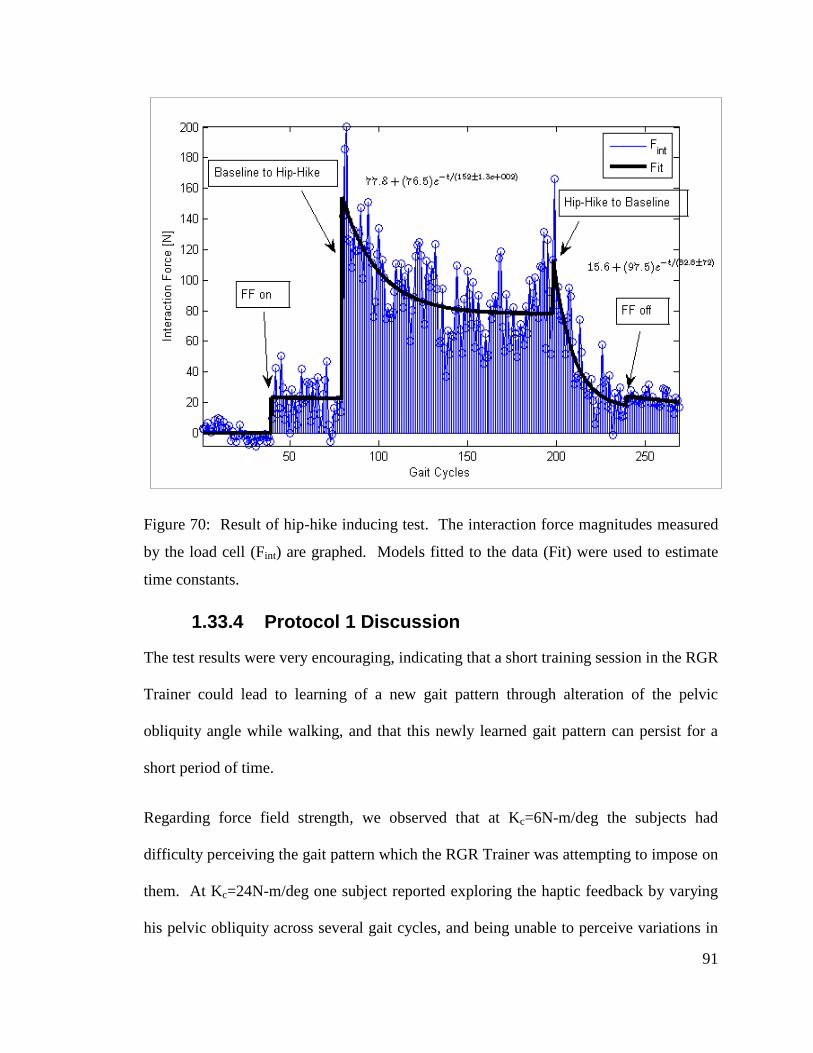
91
Figure 70: Result of hip-hike inducing test. The interaction force magnitudes measured
by the load cell (Fint) are graphed. Models fitted to the data (Fit) were used to estimate
time constants.
1.33.4 Protocol 1 Discussion
The test results were very encouraging, indicating that a short training session in the RGR
Trainer could lead to learning of a new gait pattern through alteration of the pelvic
obliquity angle while walking, and that this newly learned gait pattern can persist for a
short period of time.
Regarding force field strength, we observed that at Kc=6N-m/deg the subjects had
difficulty perceiving the gait pattern which the RGR Trainer was attempting to impose on
them. At Kc=24N-m/deg one subject reported exploring the haptic feedback by varying
his pelvic obliquity across several gait cycles, and being unable to perceive variations in
92
the force, possibly due to saturation. Reducing the force field strength to Kc = 12N-
m/deg seems to have remedied this problem, and this force field strength produced the
result shown in Figure 70. Finding the optimal force field strength to maximize retention
became one of the goals in subsequent experiments.
1.34 Protocol 2
1.34.1 Hypothesis
The success of gait retraining via force fields applied to pelvic obliquity can be judged by
the retention of the kinematics of the newly learned gait pattern in unrestricted gait
following the training period. This is in contrast to the method used in Protocol 1, where
the retention of the newly learned gait pattern was ascertained via the interaction forces
during the un-learning epoch.
1.34.2 Protocol 2 Methods
1.34.2.1 Testing Approach and Outcome Measure
As an outcome measure, the retention of the newly learned gait pattern kinematics
following the training epoch was used. After the training epoch (hip-hiking position
reference and active force field), the system was switched to backdrivable mode, with an
expectation that the subject would continue to exhibit a hip-hiking gait pattern for some
time. In an attempt to make the switch between modes less perceivable by the subject, a
tunnel around the hip-hiking reference trajectory was used. A similar tunnel has been
used by other teams, for example in [45] and [40]. The tunnel was physically
implemented in the controller by nullifying the position error while it was less than a
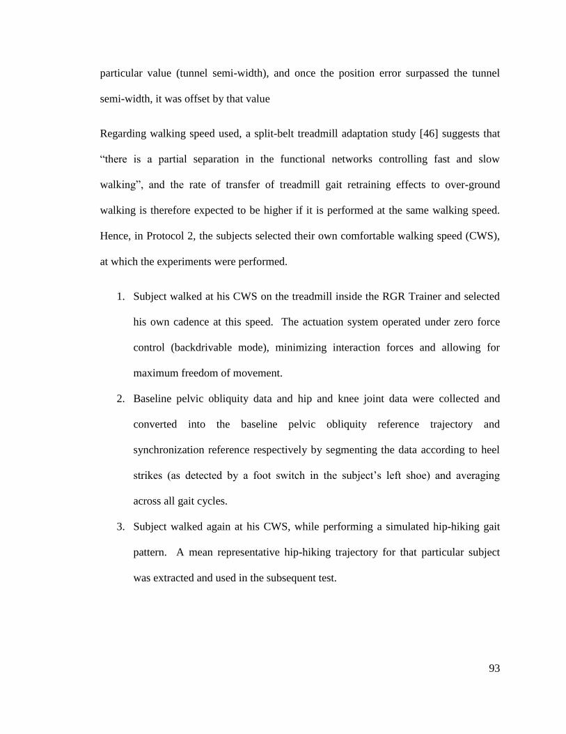
93
particular value (tunnel semi-width), and once the position error surpassed the tunnel
semi-width, it was offset by that value
Regarding walking speed used, a split-belt treadmill adaptation study [46] suggests that
“there is a partial separation in the functional networks controlling fast and slow
walking”, and the rate of transfer of treadmill gait retraining effects to over-ground
walking is therefore expected to be higher if it is performed at the same walking speed.
Hence, in Protocol 2, the subjects selected their own comfortable walking speed (CWS),
at which the experiments were performed.
1. Subject walked at his CWS on the treadmill inside the RGR Trainer and selected
his own cadence at this speed. The actuation system operated under zero force
control (backdrivable mode), minimizing interaction forces and allowing for
maximum freedom of movement.
2. Baseline pelvic obliquity data and hip and knee joint data were collected and
converted into the baseline pelvic obliquity reference trajectory and
synchronization reference respectively by segmenting the data according to heel
strikes (as detected by a foot switch in the subject’s left shoe) and averaging
across all gait cycles.
3. Subject walked again at his CWS, while performing a simulated hip-hiking gait
pattern. A mean representative hip-hiking trajectory for that particular subject
was extracted and used in the subsequent test.

94
1.34.2.2 Protocol 2
The following 4 test epochs played out to form a continuous run, as outlined in Figure 71.
The epoch durations were based on the number of gait cycles completed, as opposed to
the time elapsed as was done in Protocol 1. Throughout the test, the interaction force,
pelvic obliquity angle and gait cycle location data were recorded continuously.
4. Epoch 1. Duration: 100 gait cycles. The subject was allowed to walk freely on
the treadmill at their previously found CWS.
5. Epoch 2. Duration: 100 gait cycles. With the subject’s baseline pelvic obliquity
as the position reference, and with the tunnel size set at 1 degree (half-span), the
force field was activated.
6. Epoch 3. Duration: 300 gait cycles. The reference trajectory was switched from
the subject’s own baseline to the hip-hiking trajectory.
7. Epoch 4. Duration: 100 gait cycles. The force field was switched off. This
epoch differs from that used in Protocol 1, since the subject was not forced to
switch back to own baseline (error clamp), but was given freedom to continue
walking with the newly-acquired gait pattern. This epoch was used to record the
outcome of gait retraining, which occurred in epoch 3.
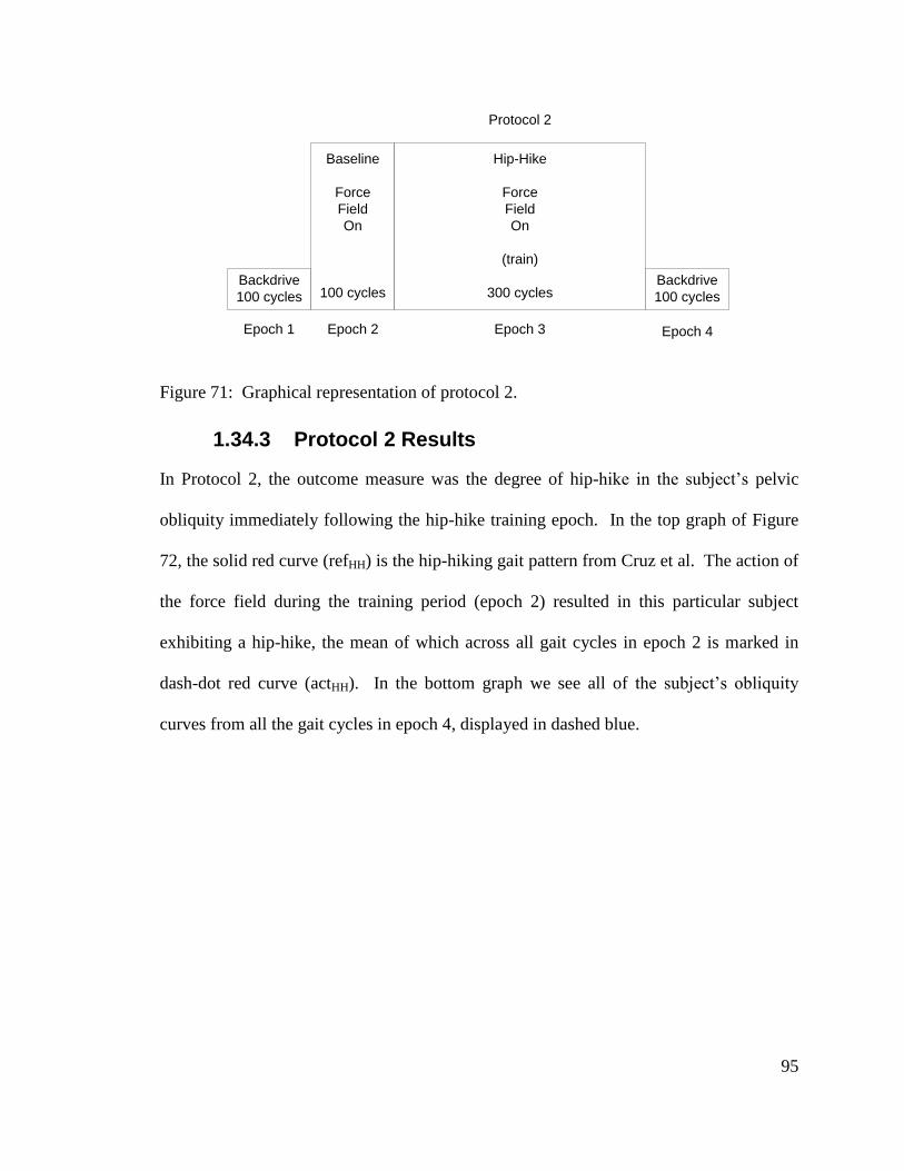
95
Backdrive
100 cycles
Baseline
Force
Field
On
100 cycles
Hip-Hike
Force
Field
On
(train)
300 cyclesBackdrive
100 cycles
Epoch 1 Epoch 2 Epoch 3 Epoch 4
Protocol 2
Figure 71: Graphical representation of protocol 2.
1.34.3 Protocol 2 Results
In Protocol 2, the outcome measure was the degree of hip-hike in the subject’s pelvic
obliquity immediately following the hip-hike training epoch. In the top graph of Figure
72, the solid red curve (refHH) is the hip-hiking gait pattern from Cruz et al. The action of
the force field during the training period (epoch 2) resulted in this particular subject
exhibiting a hip-hike, the mean of which across all gait cycles in epoch 2 is marked in
dash-dot red curve (actHH). In the bottom graph we see all of the subject’s obliquity
curves from all the gait cycles in epoch 4, displayed in dashed blue.
96
Figure 72: Sample result from one subject tested under Protocol 2. In the top graph,
refBL is the baseline pelvic obliquity of the subject, refHH is the hip-hiking trajectory from
Cruz et.al, actBL is the mean pelvic obliquity trajectory under force field, actHH is the
average hip-hiking trajectory produced by the subject under force field and actAE is the
average pelvic obliquity following hip-hike training session. In the bottom graph, pelvic
obliquity curves from all gait cycles in epoch 4 are shown (dashed blue) along with
baseline (solid black). Here one gait cycle spans between consecutive left foot toe-offs.
1.34.4 Protocol 2 Discussion
The goal of the above-described Protocol 2 experiment was to assess the RGR Trainer’s
ability to teach the hip-hiking gait pattern by the retention of the newly-learned
kinematics. By employing a ‘tunnel’ around the hip hiking reference which came from
10 20 30 40 50 60 70 80 90 100
-2
0
2
4
Percent Gait Cycle
Obliq
uity [
degre
es]
Protocol 2 Result
10 20 30 40 50 60 70 80 90 100
-2
0
2
4
Percent Gait Cycle
Obliq
uity [
degre
es]
refBL
refHH
actBL
actHH
actAE
97
the subject itself, it was expected that the perceptibility of force field removal would be
reduced, as long as the subject tracked the hip-hiking pattern closely during the training
epoch. Running this protocol at faster walking speeds meant that the hip-hiking obliquity
reference from Cruz et.al. could not be used anymore. Unfortunately, since the hip-hiking
obliquity references were collected from the subjects themselves, they were not “naïve”
to the goals of the experiment anymore. Also, despite the use of a +/- 1 degree tunnel
around the hip-hiking reference, the subjects recognized immediately the removal of the
force-field. We attempted to address these issues in Protocol 3.
1.35 Protocol 3
1.35.1 Protocol 3 Preliminary Tasks
In order to enable testing of naïve subjects at their own CWS (ca. 3km/h) with a hip-
hiking reference trajectory which would match their own simulated hip-hiking pattern
better than that found in Cruz et al. (collected at only 1.8km/h), it became necessary to
generate a representative hip-hiking trajectory (simulated by healthy subjects) collected at
the higher walking speed.
1.35.1.1 Representative Simulated Hip-hiking Obliquity Trajectory
Left and right hip-hike pelvic obliquity trajectories were collected using the RGR Trainer
under two conditions: with visual feedback and without. The tests with visual feedback
ensured that the subjects performed a hip-hike of predetermined magnitude, while the
tests without visual feedback ensured that a more representative variability in maximum
simulated hip-hike angle in healthy subjects was found. Sample plots of baseline pelvic
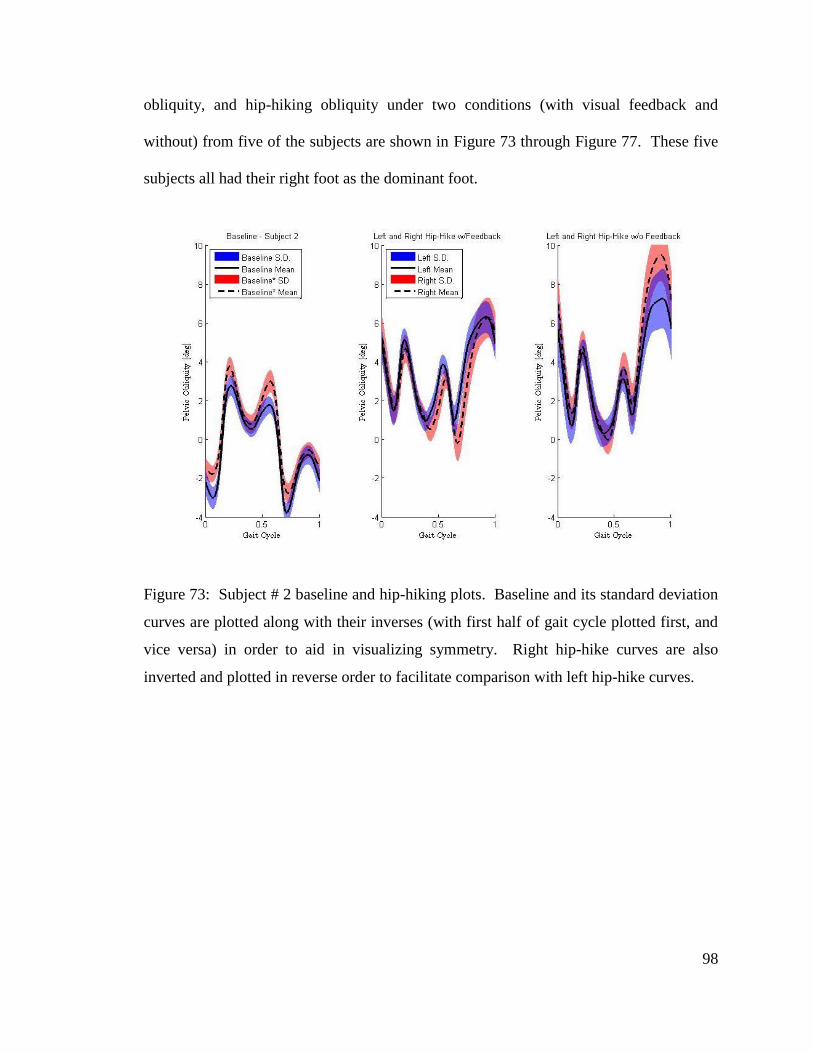
98
obliquity, and hip-hiking obliquity under two conditions (with visual feedback and
without) from five of the subjects are shown in Figure 73 through Figure 77. These five
subjects all had their right foot as the dominant foot.
Figure 73: Subject # 2 baseline and hip-hiking plots. Baseline and its standard deviation
curves are plotted along with their inverses (with first half of gait cycle plotted first, and
vice versa) in order to aid in visualizing symmetry. Right hip-hike curves are also
inverted and plotted in reverse order to facilitate comparison with left hip-hike curves.
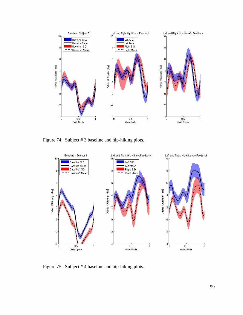
99
Figure 74: Subject # 3 baseline and hip-hiking plots.
Figure 75: Subject # 4 baseline and hip-hiking plots.
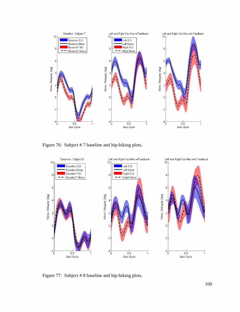
100
Figure 76: Subject # 7 baseline and hip-hiking plots.
Figure 77: Subject # 8 baseline and hip-hiking plots.
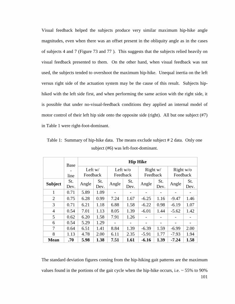
101
Visual feedback helped the subjects produce very similar maximum hip-hike angle
magnitudes, even when there was an offset present in the obliquity angle as in the cases
of subjects 4 and 7 (Figure 73 and 77 ). This suggests that the subjects relied heavily on
visual feedback presented to them. On the other hand, when visual feedback was not
used, the subjects tended to overshoot the maximum hip-hike. Unequal inertia on the left
versus right side of the actuation system may be the cause of this result. Subjects hip-
hiked with the left side first, and when performing the same action with the right side, it
is possible that under no-visual-feedback conditions they applied an internal model of
motor control of their left hip side onto the opposite side (right). All but one subject (#7)
in Table 1 were right-foot-dominant.
Table 1: Summary of hip-hike data. The means exclude subject # 2 data. Only one
subject (#6) was left-foot-dominant.
Base
-
line
Hip Hike
Left w/
Feedback
Left w/o
Feedback
Right w/
Feedback
Right w/o
Feedback
Subject St.
Dev. Angle
St.
Dev. Angle
St.
Dev. Angle
St.
Dev. Angle
St.
Dev.
1 0.71 5.89 1.09 - - - - - -
2 0.75 6.28 0.99 7.24 1.67 -6.25 1.16 -9.47 1.46
3 0.71 6.21 1.18 6.88 1.58 -6.22 0.98 -6.19 1.07
4 0.54 7.01 1.13 8.05 1.39 -6.01 1.44 -5.62 1.42
5 0.62 6.20 1.58 7.91 1.26 - - - -
6 0.54 5.29 1.29 - - - - - -
7 0.64 6.51 1.41 8.84 1.39 -6.39 1.59 -6.99 2.00
8 1.13 4.78 2.00 6.11 2.35 -5.91 1.77 -7.93 1.94
Mean .70 5.98 1.38 7.51 1.61 -6.16 1.39 -7.24 1.58
The standard deviation figures coming from the hip-hiking gait patterns are the maximum
values found in the portions of the gait cycle when the hip-hike occurs, i.e. ~ 55% to 90%
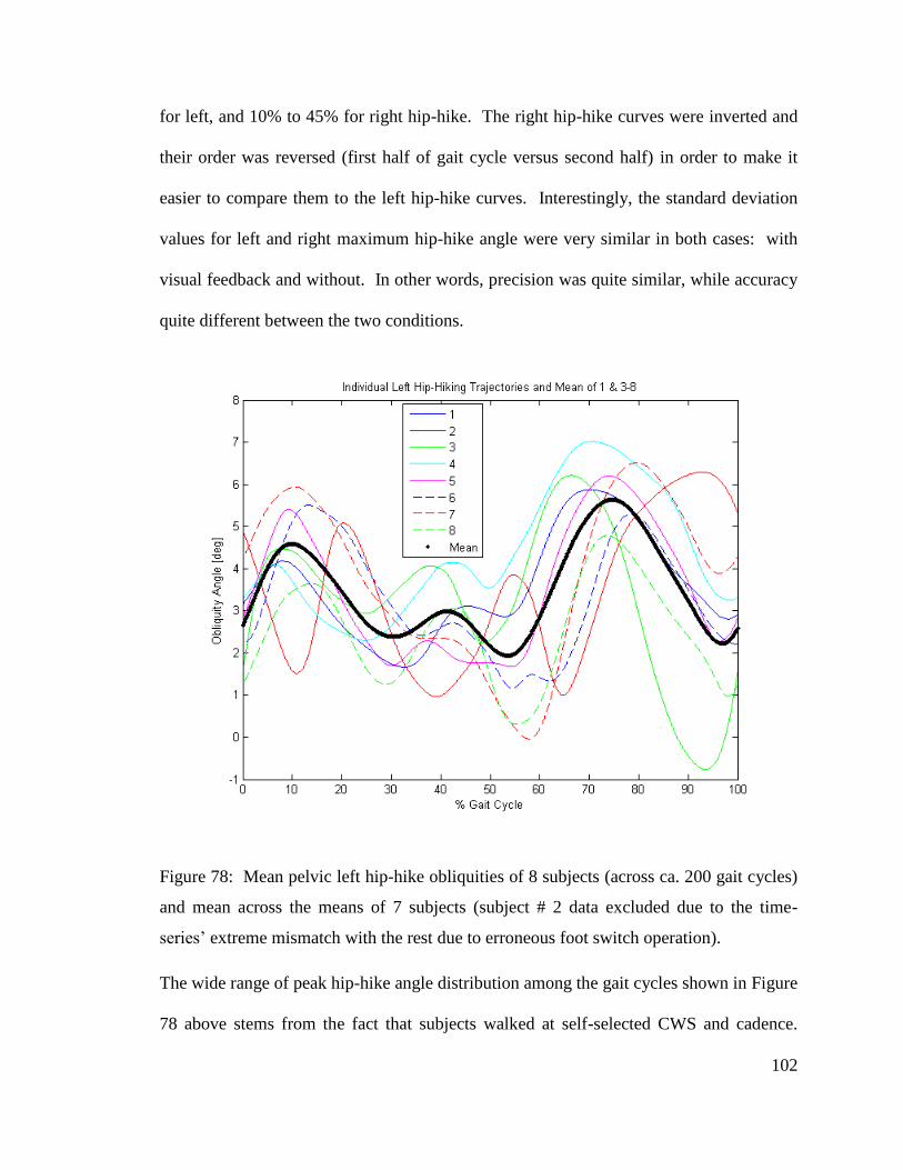
102
for left, and 10% to 45% for right hip-hike. The right hip-hike curves were inverted and
their order was reversed (first half of gait cycle versus second half) in order to make it
easier to compare them to the left hip-hike curves. Interestingly, the standard deviation
values for left and right maximum hip-hike angle were very similar in both cases: with
visual feedback and without. In other words, precision was quite similar, while accuracy
quite different between the two conditions.
Figure 78: Mean pelvic left hip-hike obliquities of 8 subjects (across ca. 200 gait cycles)
and mean across the means of 7 subjects (subject # 2 data excluded due to the time-
series’ extreme mismatch with the rest due to erroneous foot switch operation).
The wide range of peak hip-hike angle distribution among the gait cycles shown in Figure
78 above stems from the fact that subjects walked at self-selected CWS and cadence.
103
Visual feedback of maximum hip-hike angle would not be available to the subjects
during hip-hike training tests, therefore the mean of single standard deviations found in
the tests without visual feedback was used to select the tunnel size, while employing the
hip-hiking obliquity from Figure 78, which was based on tests with visual feedback,
hence featuring the appropriate maximum hip-hike magnitude of about 6 degrees. The
mentioned mean of standard deviations of maximum hip-hike angle across 7 subjects was
found to be 1.61 degrees. Therefore, it was speculated that the majority (approx. 68%) of
all the left hip-hiking gait cycles (without visual feedback) exhibited a maximum hip-hike
angle which fell within +/- 1.61 degrees of the mean. Thus we set the tunnel width to +/-
1.6 degrees.
1.35.2 Protocol 3 Methods
1.35.2.1 Outcome Measure
Selection of optimal force field strength was done based on variability of maximum hip-
hike angle. The optimal force field strength would be that of lowest magnitude, which
would produce the hip-hike angle variability σ22 which was found to be statistically
indeterminate from that of the reference trajectory.
F-test null hypothesis:
Ho: σ12 = σ2
2 (5.1)
and the alternative hypothesis:
H1: σ12 ≠ σ2 (5.2)
with a level of significance:
104
α = 0.05 (5.3)
we get the following f – values:
0.05(199,199) 1.25f (5.4)
and:
0.95
0.05
1 1(199,199) 0.8
(199,199) 1.25f
f (5.5)
Therefore, the null hypothesis is rejected when either f > 1.25 or if f < 0.8, where:
2
1
2
2
sf
s (5.6)
To confirm our assumptions, the power of the test was analyzed with G*Power software
(http://www.psycho.uni-duesseldorf.de/aap/projects/gpower/). An F-test of equality with
a detectable ratio of variances of 1.4, error probability α = 0.05, allocation ratio N1/N2 =
1 and both sample sizes of 197 each produces the power of the test of 0.651. The ratio of
variances of 1.4 is equivalent to a ratio of standard deviations of 1.183.
1.35.2.2 Protocol 3 Setup
1. Subject walked at his CWS on the treadmill inside the RGR Trainer and selected
his own cadence at this speed. The actuation system operated under zero force
control (backdrivable mode), minimizing interaction forces and allowing for
maximum freedom of movement.
2. Baseline pelvic obliquity data and hip and knee joint data were collected by
recording the RGR Trainer’s pelvic brace position measurement and hip and knee
angle measurements, and converted into the baseline pelvic obliquity reference

105
trajectory and synchronization reference respectively by segmenting the data
according to heel strikes (as detected by a foot switch in the subject’s left shoe),
and averaging across all gait cycles.
1.35.2.3 Protocol 3 Details
Five different force field levels (Kc = 20, 25, 30, 35 and 40N-m/deg) were randomized.
3. Epoch 1. Duration 50 gait cycles. The subject ambulated, and reached a steady
state pace.
4. Epoch 2. Duration 300 gait cycles. Subject was exposed to a force field
selected randomly out of 5, with the representative hip-hike pattern serving as the
position trajectory, activated between 55% and 85% of the gait cycle. A previous
test result (Figure 70) suggested a time constant of about 150 gait cycles,
therefore here twice the time-constant was used: 300 gait cycles.
5. Epoch 3. Duration 200 gait cycles. The 200 cycles were used to record the
outcome of gait retraining.
6. Epoch 4. Duration 300 gait cycles. An error-clamp setting, with tunnel set to
+/- 0.7 degrees and a force field of K = 30 N-m/deg was used. 0.7 degrees is the
single standard deviation of the mean of baseline obliquities of seven subjects
from Table 1.
7. Epoch 5. Duration 200 gait cycles. Force field was off. Obliquity from this
epoch was used to confirm that de-adaptation was sufficient. One potential
method was computing the sample variance s22 and performing an F-test against
reference (baseline) variance.
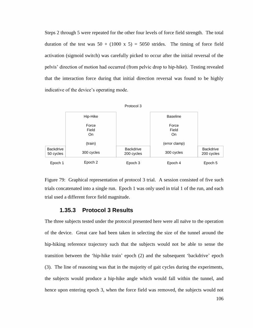
106
Steps 2 through 5 were repeated for the other four levels of force field strength. The total
duration of the test was 50 + (1000 x 5) = 5050 strides. The timing of force field
activation (sigmoid switch) was carefully picked to occur after the initial reversal of the
pelvis’ direction of motion had occurred (from pelvic drop to hip-hike). Testing revealed
that the interaction force during that initial direction reversal was found to be highly
indicative of the device’s operating mode.
Backdrive
50 cycles
Hip-Hike
Force
Field
On
(train)
300 cycles
Epoch 1 Epoch 2 Epoch 3
Protocol 3
Baseline
Force
Field
On
(error clamp)
300 cycles
Epoch 4 Epoch 5
Backdrive
200 cycles
Backdrive
200 cycles
Figure 79: Graphical representation of protocol 3 trial. A session consisted of five such
trials concatenated into a single run. Epoch 1 was only used in trial 1 of the run, and each
trial used a different force field magnitude.
1.35.3 Protocol 3 Results
The three subjects tested under the protocol presented here were all naïve to the operation
of the device. Great care had been taken in selecting the size of the tunnel around the
hip-hiking reference trajectory such that the subjects would not be able to sense the
transition between the ‘hip-hike train’ epoch (2) and the subsequent ‘backdrive’ epoch
(3). The line of reasoning was that in the majority of gait cycles during the experiments,
the subjects would produce a hip-hike angle which would fall within the tunnel, and
hence upon entering epoch 3, when the force field was removed, the subjects would not
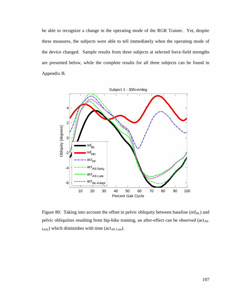
107
be able to recognize a change in the operating mode of the RGR Trainer. Yet, despite
these measures, the subjects were able to tell immediately when the operating mode of
the device changed. Sample results from three subjects at selected force-field strengths
are presented below, while the complete results for all three subjects can be found in
Appendix B.
Figure 80: Taking into account the offset in pelvic obliquity between baseline (refBL) and
pelvic obliquities resulting from hip-hike training, an after-effect can be observed (actAE-
Early) which diminishes with time (actAE-Late).
10 20 30 40 50 60 70 80 90 100
-6
-4
-2
0
2
4
Percent Gait Cycle
Obliq
uity [
degre
es]
Subject 1 - 30N-m/deg
refBL
refHH
actFF
actAE-Early
actAE-Late
actde-Adapt
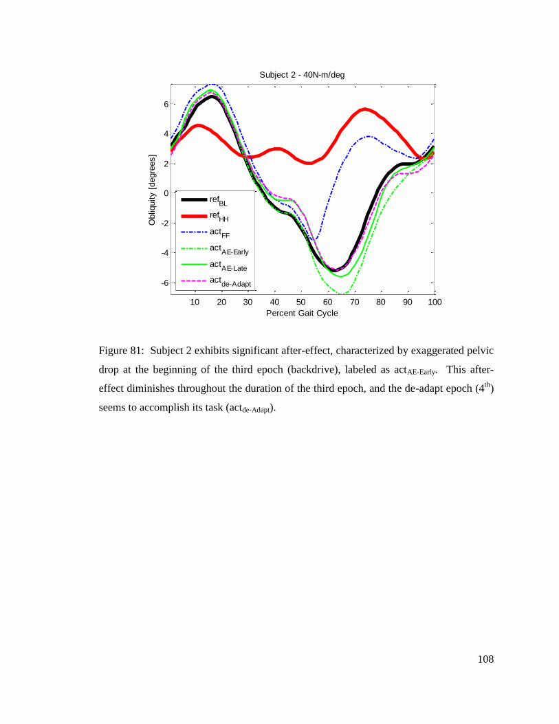
108
Figure 81: Subject 2 exhibits significant after-effect, characterized by exaggerated pelvic
drop at the beginning of the third epoch (backdrive), labeled as actAE-Early. This after-
effect diminishes throughout the duration of the third epoch, and the de-adapt epoch (4th
)
seems to accomplish its task (actde-Adapt).
10 20 30 40 50 60 70 80 90 100
-6
-4
-2
0
2
4
6
Percent Gait Cycle
Obliq
uity [
degre
es]
Subject 2 - 40N-m/deg
refBL
refHH
actFF
actAE-Early
actAE-Late
actde-Adapt
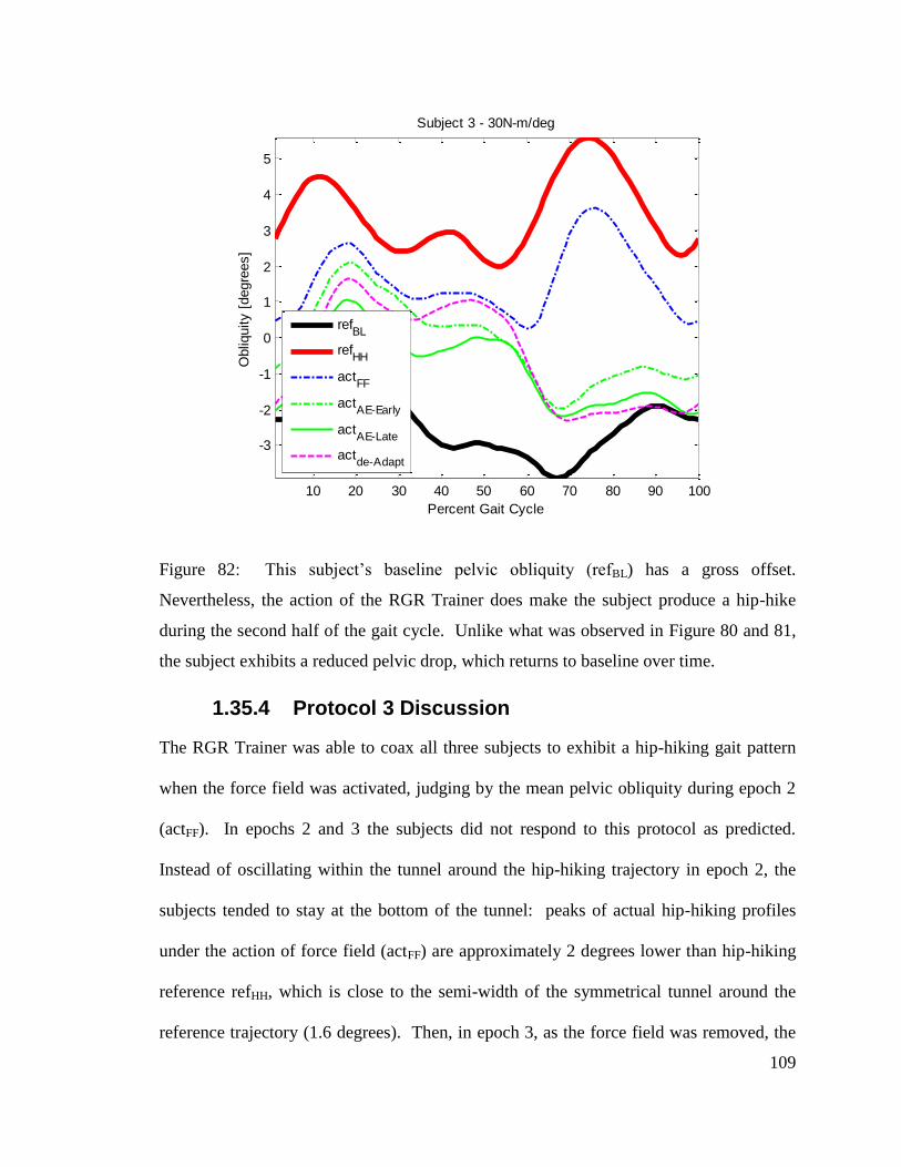
109
Figure 82: This subject’s baseline pelvic obliquity (refBL) has a gross offset.
Nevertheless, the action of the RGR Trainer does make the subject produce a hip-hike
during the second half of the gait cycle. Unlike what was observed in Figure 80 and 81,
the subject exhibits a reduced pelvic drop, which returns to baseline over time.
1.35.4 Protocol 3 Discussion
The RGR Trainer was able to coax all three subjects to exhibit a hip-hiking gait pattern
when the force field was activated, judging by the mean pelvic obliquity during epoch 2
(actFF). In epochs 2 and 3 the subjects did not respond to this protocol as predicted.
Instead of oscillating within the tunnel around the hip-hiking trajectory in epoch 2, the
subjects tended to stay at the bottom of the tunnel: peaks of actual hip-hiking profiles
under the action of force field (actFF) are approximately 2 degrees lower than hip-hiking
reference refHH, which is close to the semi-width of the symmetrical tunnel around the
reference trajectory (1.6 degrees). Then, in epoch 3, as the force field was removed, the
10 20 30 40 50 60 70 80 90 100
-3
-2
-1
0
1
2
3
4
5
Percent Gait Cycle
Obliq
uity [
degre
es]
Subject 3 - 30N-m/deg
refBL
refHH
actFF
actAE-Early
actAE-Late
actde-Adapt
110
subjects gradually stopped hip-hiking, but this change did not occur subconsciously,
because the subjects immediately realized that the force field was removed. Therefore, it
was biased by the subjects’ motivation and understanding of their task. As a result of the
subjects hip-hiking at the bottom of the reference tunnel and interacting with the force
field, the removal of the force field in epoch 3 produced a sensation of a downward-
directed force, which in turn caused the subjects to exhibit an increased pelvic drop, as
compared to their baseline pelvic obliquity. In other words, while these experiments
were assistive in nature, and the subjects were instructed to follow the guidance, the
subjects adapted to the forces present in epoch 2, and they de-adapted in epoch 3, i.e. they
underwent motor adaptation.
1.36 Protocol 4
1.36.1 Introduction
Protocols 2 and 3 attempted to quantify the effectiveness of assistive gait retraining
strategies with the retention levels of the newly acquired gait pattern. Implementing a
protocol which measures gait pattern retention which is unbiased by subjects’ motivation
proved to be very challenging. Protocol 4 aimed to investigate motor control of the
pelvis by comparing both assistive and resistive training.
1.36.2 Protocol 4 Methods
Four healthy subjects participated in the study. Each subject completed two assistive and
two resistive training sessions. During the assistive training sessions, the subjects were
instructed to follow the guidance of the RGR Trainer, and during the resistive sessions,
the subjects were instructed to maintain their own natural gait pattern and not to allow the
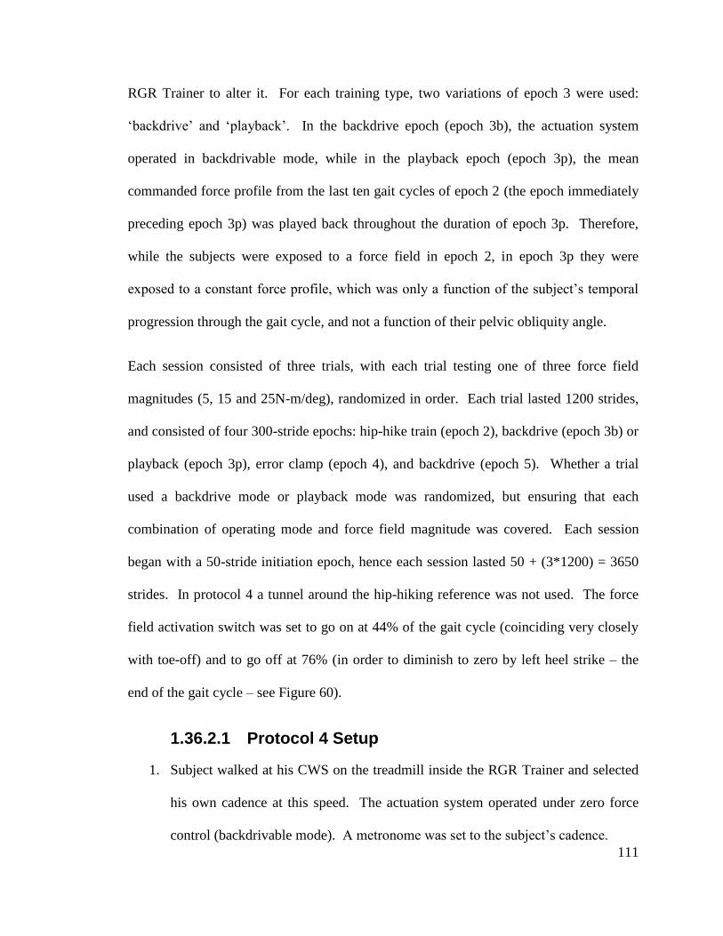
111
RGR Trainer to alter it. For each training type, two variations of epoch 3 were used:
‘backdrive’ and ‘playback’. In the backdrive epoch (epoch 3b), the actuation system
operated in backdrivable mode, while in the playback epoch (epoch 3p), the mean
commanded force profile from the last ten gait cycles of epoch 2 (the epoch immediately
preceding epoch 3p) was played back throughout the duration of epoch 3p. Therefore,
while the subjects were exposed to a force field in epoch 2, in epoch 3p they were
exposed to a constant force profile, which was only a function of the subject’s temporal
progression through the gait cycle, and not a function of their pelvic obliquity angle.
Each session consisted of three trials, with each trial testing one of three force field
magnitudes (5, 15 and 25N-m/deg), randomized in order. Each trial lasted 1200 strides,
and consisted of four 300-stride epochs: hip-hike train (epoch 2), backdrive (epoch 3b) or
playback (epoch 3p), error clamp (epoch 4), and backdrive (epoch 5). Whether a trial
used a backdrive mode or playback mode was randomized, but ensuring that each
combination of operating mode and force field magnitude was covered. Each session
began with a 50-stride initiation epoch, hence each session lasted 50 + (3*1200) = 3650
strides. In protocol 4 a tunnel around the hip-hiking reference was not used. The force
field activation switch was set to go on at 44% of the gait cycle (coinciding very closely
with toe-off) and to go off at 76% (in order to diminish to zero by left heel strike – the
end of the gait cycle – see Figure 60).
1.36.2.1 Protocol 4 Setup
1. Subject walked at his CWS on the treadmill inside the RGR Trainer and selected
his own cadence at this speed. The actuation system operated under zero force
control (backdrivable mode). A metronome was set to the subject’s cadence.

112
2. As the subject ambulated for 100 gait cycles to the cadence set by the metronome,
baseline pelvic obliquity timeseries and hip and knee joint angle timeseries were
collected and converted into the baseline pelvic obliquity reference trajectory and
synchronization reference respectively, by segmenting the data according to heel
strikes (as detected by a foot switch in the subject’s left shoe), and averaging
across all gait cycles.
1.36.2.2 Protocol 4 Details
3. With the metronome setting the cadence, the subject ambulated in the RGR
Trainer for 5 minutes, with the system in backdrivable mode in order to reach
steady state.
4. Epoch 1. Duration 50 gait cycles. Initiation: every 5 strides, the RGR Trainer
switched between two operating modes: error clamp (baseline reference) and hip-
hike train. This was done to make the subjects accustomed to the operation of the
system, and to make subjects believe that there are only two operating modes.
5. Epoch 2. Duration 300 gait cycles. Subject was exposed to a force field
selected randomly out of 3, with the representative hip-hike pattern serving as the
position trajectory, activated between 44% and 76% of the gait cycle.
6. Epoch 3b. Duration 300 gait cycles. The system operated in backdrivable
mode.
7. Epoch 3p. Duration 300 gait cycles. The system operated in playback mode,
generating a constant force profile (mean commanded force from last 10 gait
cycles in epoch 2) as a function of temporal progression through the gait cycle.
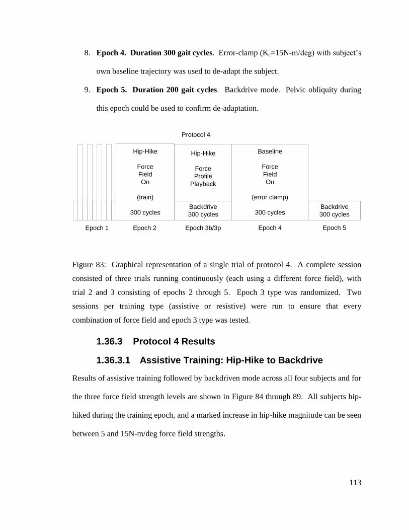
113
8. Epoch 4. Duration 300 gait cycles. Error-clamp (Kc=15N-m/deg) with subject’s
own baseline trajectory was used to de-adapt the subject.
9. Epoch 5. Duration 200 gait cycles. Backdrive mode. Pelvic obliquity during
this epoch could be used to confirm de-adaptation.
Hip-Hike
Force
Field
On
(train)
300 cycles
Epoch 1 Epoch 2 Epoch 3b/3p
Protocol 4
Baseline
Force
Field
On
(error clamp)
300 cycles
Epoch 4 Epoch 5
Backdrive
300 cycles
Backdrive
300 cycles
Hip-Hike
Force
Profile
Playback
Figure 83: Graphical representation of a single trial of protocol 4. A complete session
consisted of three trials running continuously (each using a different force field), with
trial 2 and 3 consisting of epochs 2 through 5. Epoch 3 type was randomized. Two
sessions per training type (assistive or resistive) were run to ensure that every
combination of force field and epoch 3 type was tested.
1.36.3 Protocol 4 Results
1.36.3.1 Assistive Training: Hip-Hike to Backdrive
Results of assistive training followed by backdriven mode across all four subjects and for
the three force field strength levels are shown in Figure 84 through 89. All subjects hip-
hiked during the training epoch, and a marked increase in hip-hike magnitude can be seen
between 5 and 15N-m/deg force field strengths.
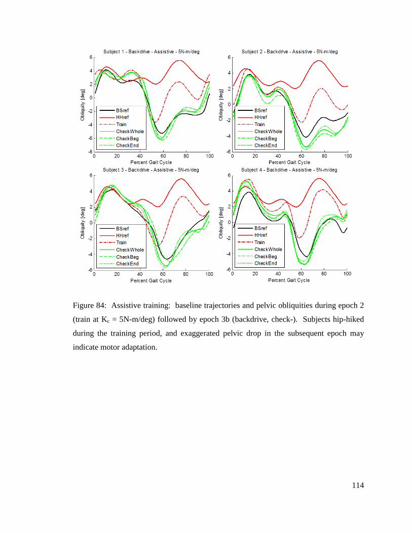
114
Figure 84: Assistive training: baseline trajectories and pelvic obliquities during epoch 2
(train at Kc = 5N-m/deg) followed by epoch 3b (backdrive, check-). Subjects hip-hiked
during the training period, and exaggerated pelvic drop in the subsequent epoch may
indicate motor adaptation.
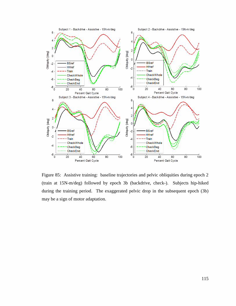
115
Figure 85: Assistive training: baseline trajectories and pelvic obliquities during epoch 2
(train at 15N-m/deg) followed by epoch 3b (backdrive, check-). Subjects hip-hiked
during the training period. The exaggerated pelvic drop in the subsequent epoch (3b)
may be a sign of motor adaptation.
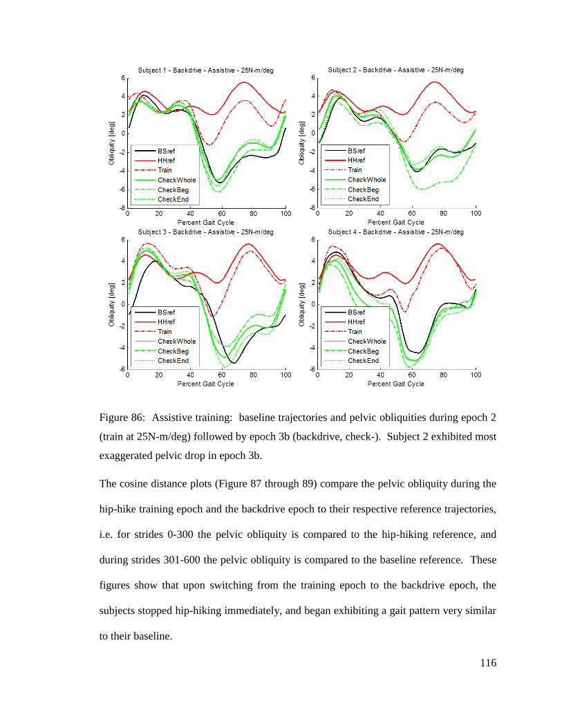
116
Figure 86: Assistive training: baseline trajectories and pelvic obliquities during epoch 2
(train at 25N-m/deg) followed by epoch 3b (backdrive, check-). Subject 2 exhibited most
exaggerated pelvic drop in epoch 3b.
The cosine distance plots (Figure 87 through 89) compare the pelvic obliquity during the
hip-hike training epoch and the backdrive epoch to their respective reference trajectories,
i.e. for strides 0-300 the pelvic obliquity is compared to the hip-hiking reference, and
during strides 301-600 the pelvic obliquity is compared to the baseline reference. These
figures show that upon switching from the training epoch to the backdrive epoch, the
subjects stopped hip-hiking immediately, and began exhibiting a gait pattern very similar
to their baseline.
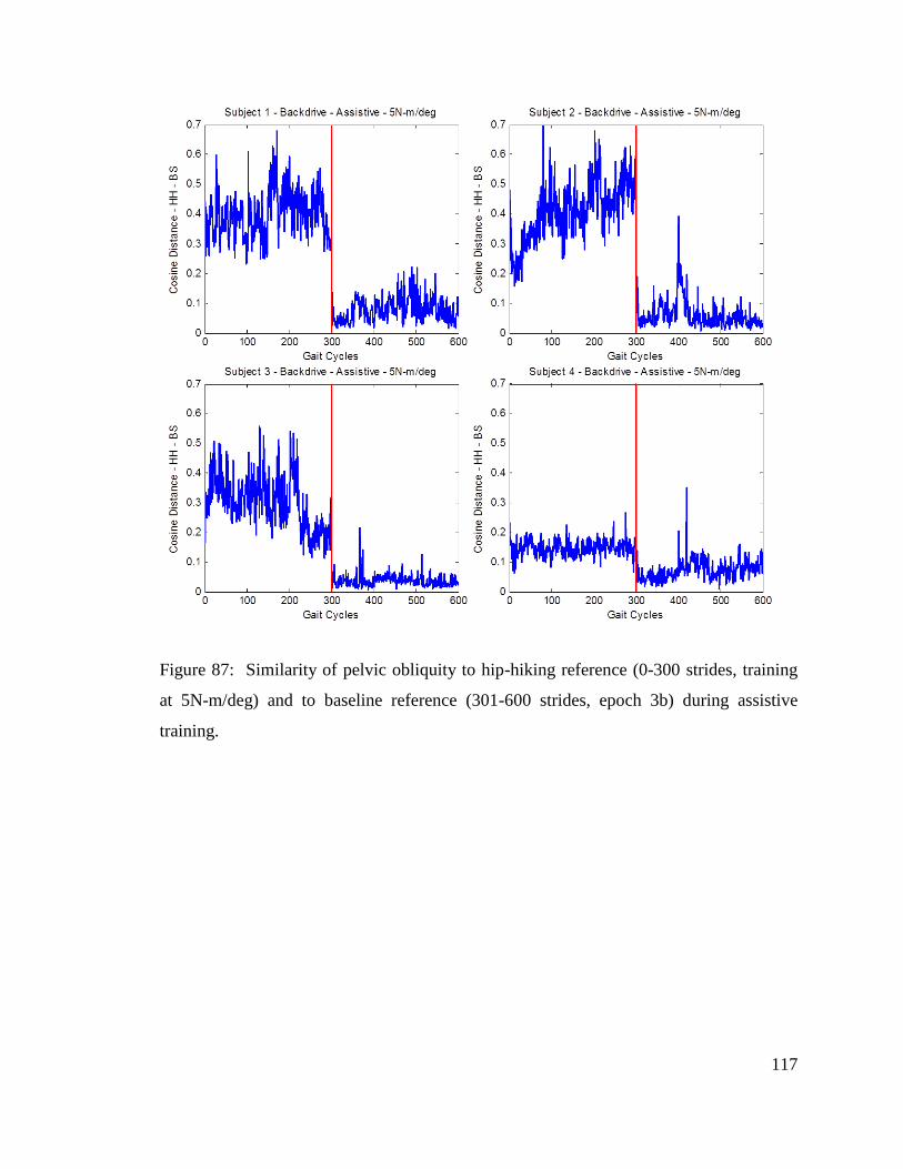
117
Figure 87: Similarity of pelvic obliquity to hip-hiking reference (0-300 strides, training
at 5N-m/deg) and to baseline reference (301-600 strides, epoch 3b) during assistive
training.
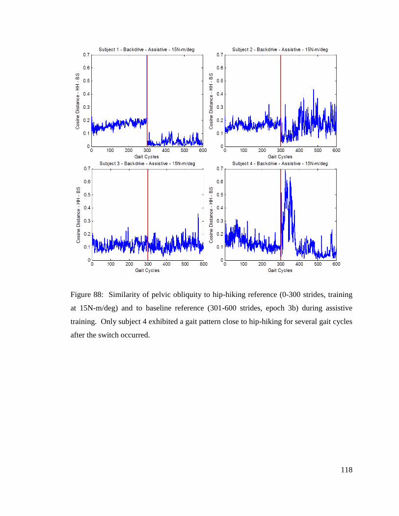
118
Figure 88: Similarity of pelvic obliquity to hip-hiking reference (0-300 strides, training
at 15N-m/deg) and to baseline reference (301-600 strides, epoch 3b) during assistive
training. Only subject 4 exhibited a gait pattern close to hip-hiking for several gait cycles
after the switch occurred.
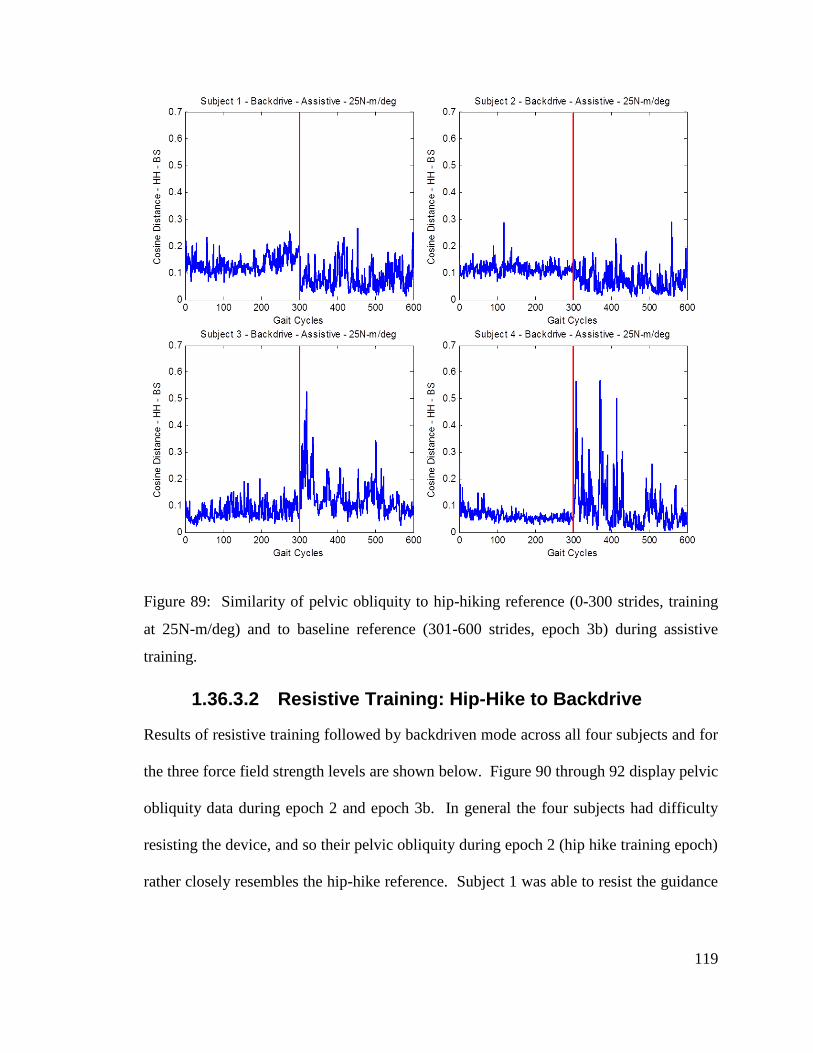
119
Figure 89: Similarity of pelvic obliquity to hip-hiking reference (0-300 strides, training
at 25N-m/deg) and to baseline reference (301-600 strides, epoch 3b) during assistive
training.
1.36.3.2 Resistive Training: Hip-Hike to Backdrive
Results of resistive training followed by backdriven mode across all four subjects and for
the three force field strength levels are shown below. Figure 90 through 92 display pelvic
obliquity data during epoch 2 and epoch 3b. In general the four subjects had difficulty
resisting the device, and so their pelvic obliquity during epoch 2 (hip hike training epoch)
rather closely resembles the hip-hike reference. Subject 1 was able to resist the guidance
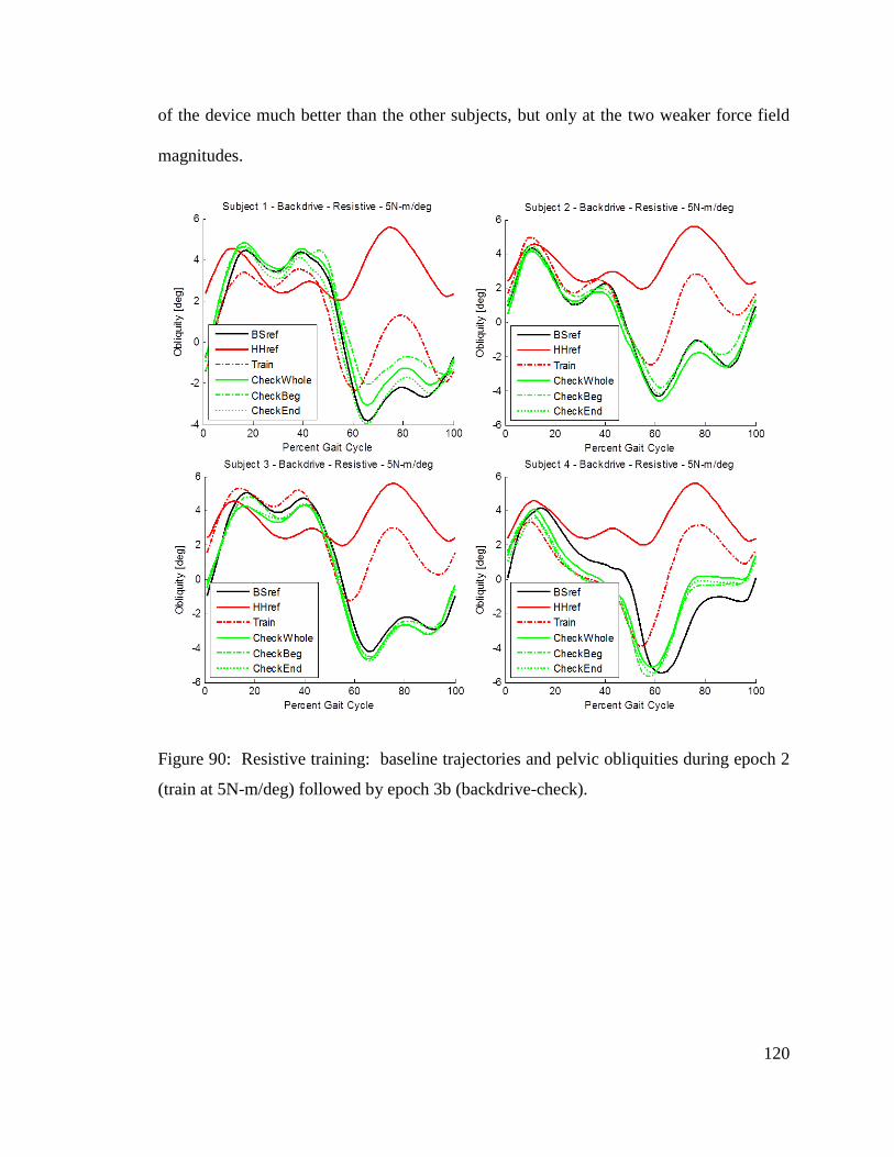
120
of the device much better than the other subjects, but only at the two weaker force field
magnitudes.
Figure 90: Resistive training: baseline trajectories and pelvic obliquities during epoch 2
(train at 5N-m/deg) followed by epoch 3b (backdrive-check).
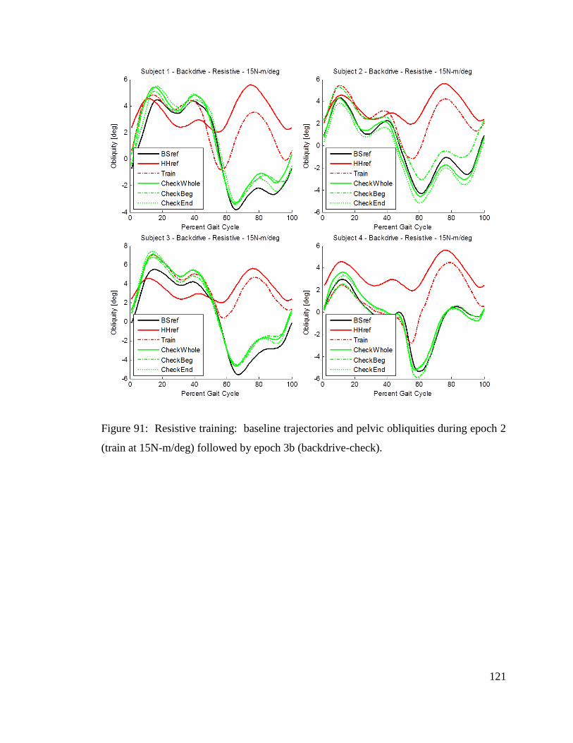
121
Figure 91: Resistive training: baseline trajectories and pelvic obliquities during epoch 2
(train at 15N-m/deg) followed by epoch 3b (backdrive-check).
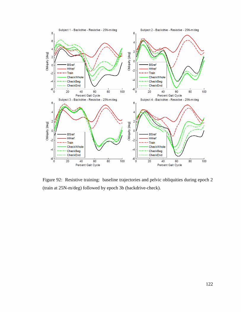
122
Figure 92: Resistive training: baseline trajectories and pelvic obliquities during epoch 2
(train at 25N-m/deg) followed by epoch 3b (backdrive-check).
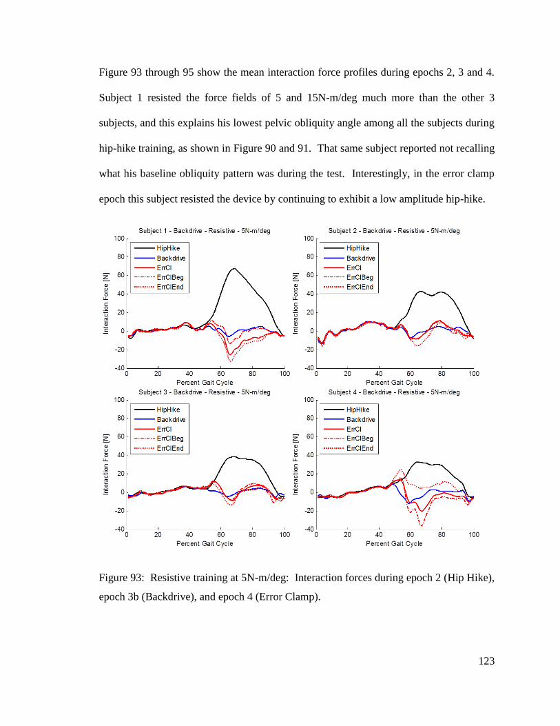
123
Figure 93 through 95 show the mean interaction force profiles during epochs 2, 3 and 4.
Subject 1 resisted the force fields of 5 and 15N-m/deg much more than the other 3
subjects, and this explains his lowest pelvic obliquity angle among all the subjects during
hip-hike training, as shown in Figure 90 and 91. That same subject reported not recalling
what his baseline obliquity pattern was during the test. Interestingly, in the error clamp
epoch this subject resisted the device by continuing to exhibit a low amplitude hip-hike.
Figure 93: Resistive training at 5N-m/deg: Interaction forces during epoch 2 (Hip Hike),
epoch 3b (Backdrive), and epoch 4 (Error Clamp).
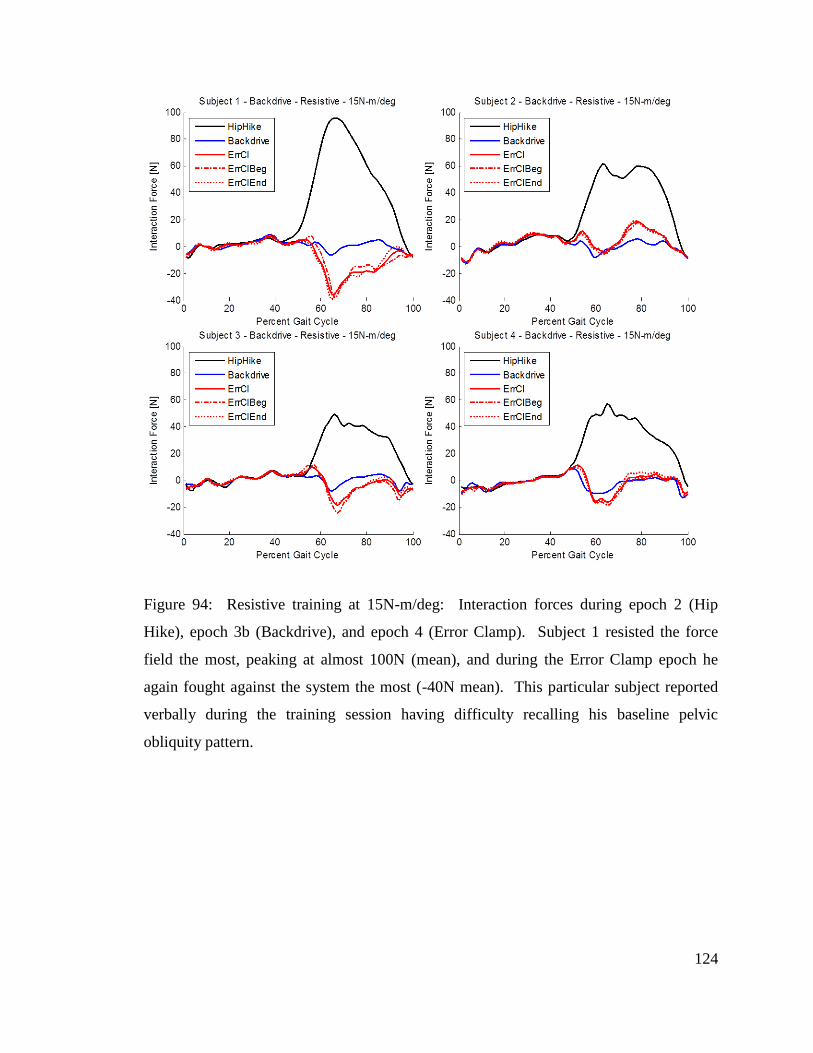
124
Figure 94: Resistive training at 15N-m/deg: Interaction forces during epoch 2 (Hip
Hike), epoch 3b (Backdrive), and epoch 4 (Error Clamp). Subject 1 resisted the force
field the most, peaking at almost 100N (mean), and during the Error Clamp epoch he
again fought against the system the most (-40N mean). This particular subject reported
verbally during the training session having difficulty recalling his baseline pelvic
obliquity pattern.
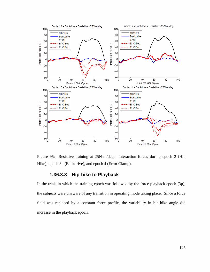
125
Figure 95: Resistive training at 25N-m/deg: Interaction forces during epoch 2 (Hip
Hike), epoch 3b (Backdrive), and epoch 4 (Error Clamp).
1.36.3.3 Hip-hike to Playback
In the trials in which the training epoch was followed by the force playback epoch (3p),
the subjects were unaware of any transition in operating mode taking place. Since a force
field was replaced by a constant force profile, the variability in hip-hike angle did
increase in the playback epoch.
126
1.36.4 Protocol 4 Discussion
1.36.4.1 Assistive Training followed by Backdrive
Though the combination of assistive hip-hike training followed by backdrivable epoch
had been used in Protocol 3, it was repeated here so that the assistive and resistive
training paradigms could be compared and contrasted. This time no attempt was made to
conceal the transition between the two epochs; no tunnel was used, and the sigmoid was
turned on at 44%, coinciding with the left toe-off, which resulted in increasing the effect
that force field had on hip-hike generation. The RGR Trainer caused all subjects to hip-
hike during epoch 2 (Figure 84 through 86), but turning the force-field off resulted in
immediate switch to baseline obliquity gait pattern (Figure 87 through 89). In fact in the
majority of the trials the subjects exhibited an exaggerated pelvic drop, and all subjects
stated that the device was ‘pushing them down’ when the system switched from the
training epoch to the backdrive epoch. This sensation may be explained by the subjects
both getting accustomed to the haptic feedback and by the subjects adopting a new gait
pattern during the training period. This result suggests that some subjects experienced
motor adaptation and de-adaptation. Motor adaptations in studies are usually evoked
through resistive training [37, 38, 40, 42, 43], but the fact that during assistive training
the subjects still experienced significant forces (judging by position error in Figure 84
thru 86) could explain why there are signs of motor adaptations. The significant position
error in assistive training also suggests that hip-hiking up to 6 degrees of rotation makes
the gait pattern very inefficient and uncomfortable.
127
1.36.4.2 Resistive Training followed by Backdrive
Resistive training produced rather surprising results. Despite being instructed to not
allow the device to alter their gait pattern, in the majority of the trials the subjects did hip-
hike. One notable exception is the trial at 5N-m/deg with subject 1. This subject was
able to keep the hip-hike angle to a much lower magnitude than the other subjects.
Though in assistive training we observed a trend of increased pelvic drop in the backdrive
epoch among some subjects and trials, resistive training seems to have had the opposite
effect, although it is not consistent across all subjects and all force field strength levels.
There seems to be a correlation between the effort put into resisting hip-hiking during
epoch 2 and the magnitude of hip-hike angle in epoch 3b. Subjects 1 and 3 produced the
smallest hip-hike magnitudes during epoch 2, and subsequently produced the smallest
pelvic drop magnitudes in epoch 3b (i.e. they exhibited a small hip-hike).
1.37 Conclusion
The four test protocols presented in this chapter describe the evolution of approaches,
which were used to investigate the RGR Trainer’s ability to administer gait retraining to
healthy subjects. Experiments with all four protocols demonstrated the system’s ability
to alter healthy subjects’ gait by applying a moment to pelvic obliquity to cause hip-
hiking, and signs of retention of the gait patterns being trained were observed in many of
the subjects tested with the four protocols. Retention of newly learned motor patterns has
been stated as the proof of motor learning in experiments with upper and lower
extremities [37, 38, 40-43], and studies with stroke survivors [37, 43] have found that
adapting the patient to a perturbation that worsened or amplified their error was what
128
drove adaptation to result in after-effects that improved their movement. The
experiments with protocols 1 through 3 and half of the experiments with protocol 4 were
assistive in nature, where the subjects were instructed to let the device guide their pelvis.
Only protocol 4 included resistive training. It is the resistive training paradigm which
most motor learning studies have relied on to assess motor adaptations. In resistive
training of protocol 4, subjects were instructed to resist the guidance of the RGR Trainer
(which was imposing on them the hip-hiking gait pattern) and to maintain their own gait
pattern, which means exhibiting pelvic drop during leg swing. The results of resistive
training presented here indicate that in the majority of the trials the subjects were not
actively engaging in exhibiting pelvic drop in their gait pattern. It may be the case that
pelvic drop occurs passively, due to upper body’s weight, which would mean that
humans don’t normally engage muscles of the lower body to ‘drive’ the pelvic drop.
Therefore, the results of the study using protocol 4 in regards to motor control of the
pelvis are not conclusive, and further testing with redesigned protocols will have to be
performed in the future.
129
Conclusions
1.38 Summary
Stroke is a leading cause of disability in America, severely affecting victim’s locomotion.
Manual gait rehabilitation is costly and physically demanding, which led to an increased
interest in robotic devices. Nevertheless, one limitation which the commercially
available robotic devices for rehabilitation seem to share is constraint of the natural
pelvic motions. Addressing of both primary gait deviations in the legs as well as the
secondary gait deviations in the pelvis (which arise as compensatory movements to the
primary gait deviations) may offer a much needed improvement in the outcome of gait
retraining following stroke.
Therefore, the Robotic Gait Rehabilitation (RGR) Trainer was designed and built to be a
simple, low cost device with a single actuator, which allows all the natural motions of the
pelvis, while being able to selectively and compliantly guide the pelvis in the frontal
plane (pelvic obliquity) in order to target hip-hiking in patients post stroke. This device
uses impedance control and human-machine synchronization to generate corrective
forces as a response to deviations from pre-determined pelvic obliquity trajectories. The
corrective forces are transferred to the subject via a lower body exoskeleton, which can
very effectively transfer forces to the pelvis, while its 10 DOFs allow for unhindered
ambulation on the treadmill.
Testing of several healthy subjects using four different protocols has demonstrated that
the RGR Trainer can effectively alter the gait by imposing a hip-hiking gait pattern, and
130
retention of this gait patter has been observed following the training sessions, which
implies learning. The qualities of the RGR Trainer make it a very good tool for the study
of motor control of the pelvis, the understanding of which is expected to lead to designing
better gait retraining strategies in the future.
1.39 Future Work
1.39.1 Mechanical Design
One minor hardware upgrade, which may improve both the range of motion of the
actuation system and the performance of the control system is the replacement of the
linear potentiometer, which is used with the linear actuator position measurement to
compute pelvic obliquity angle. Installation of a digital linear encoder with proper range
of motion would eliminate the electrical noise inherent to analog devices, and therefore
possibly increase the operating range of the impedance controller.
The first major mechanical upgrade of the system will be the addition of an assembly,
which is referred to as the horizontal motion system in section 1.14. This assembly
increases the range of lateral motion of the subject in the device, and it shifts the location
of the subject forward of the main frame. This will give a physical therapists unrestricted
access to the patients’ legs for assisting with stepping and knee flexion.
Extending the operating envelope of the RGR Trainer to pelvic rotation will require
another major upgrade of the mechanical system. One possible design, which uses four
linear actuators to control 2 rotational DOFs of the pelvis is presented in Appendix C -
RGR Trainer 2DOF.
131
1.39.2 Control Strategies and Software
Many unforeseeable problems are likely to arise due to testing of patients post-stroke in
the RGR Trainer, but one issue which is very likely to appear will be lower accuracy of
the human-machine synchronization system’s gait cycle location estimate. This problem
is expected to arise mainly due to pronounced gait asymmetries in patients, as well as a
more dramatic modification of gait parameters within a training session. Therefore, the
human-machine synchronization algorithm will have to be developed further, for
example by the addition of weight assignment to the 8 DOFs currently used, such that the
system becomes more resilient to perturbations.
1.39.3 Human Testing
Healthy subject testing presented in 0 demonstrated the RGR Trainer’s ability to
effectively and reliably apply corrective force fields to pelvic obliquity. This work has
laid down a foundation for future experiments, which will try to answer more directly
questions about motor control of the pelvis. These experiments will in turn allow for
further testing to take place with patients post-stroke, which will demonstrate the efficacy
of addressing secondary gait deviations in gait retraining.
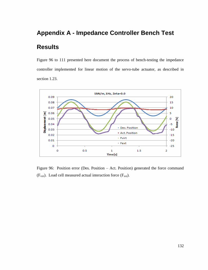
132
Appendix A - Impedance Controller Bench Test
Results
Figure 96 to 111 presented here document the process of bench-testing the impedance
controller implemented for linear motion of the servo-tube actuator, as described in
section 1.23.
Figure 96: Position error (Des. Position – Act. Position) generated the force command
(Fvirt). Load cell measured actual interaction force (Fext).
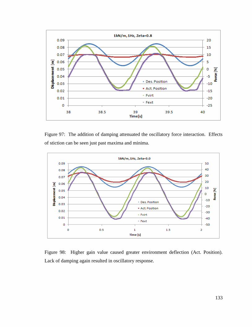
133
Figure 97: The addition of damping attenuated the oscillatory force interaction. Effects
of stiction can be seen just past maxima and minima.
Figure 98: Higher gain value caused greater environment deflection (Act. Position).
Lack of damping again resulted in oscillatory response.
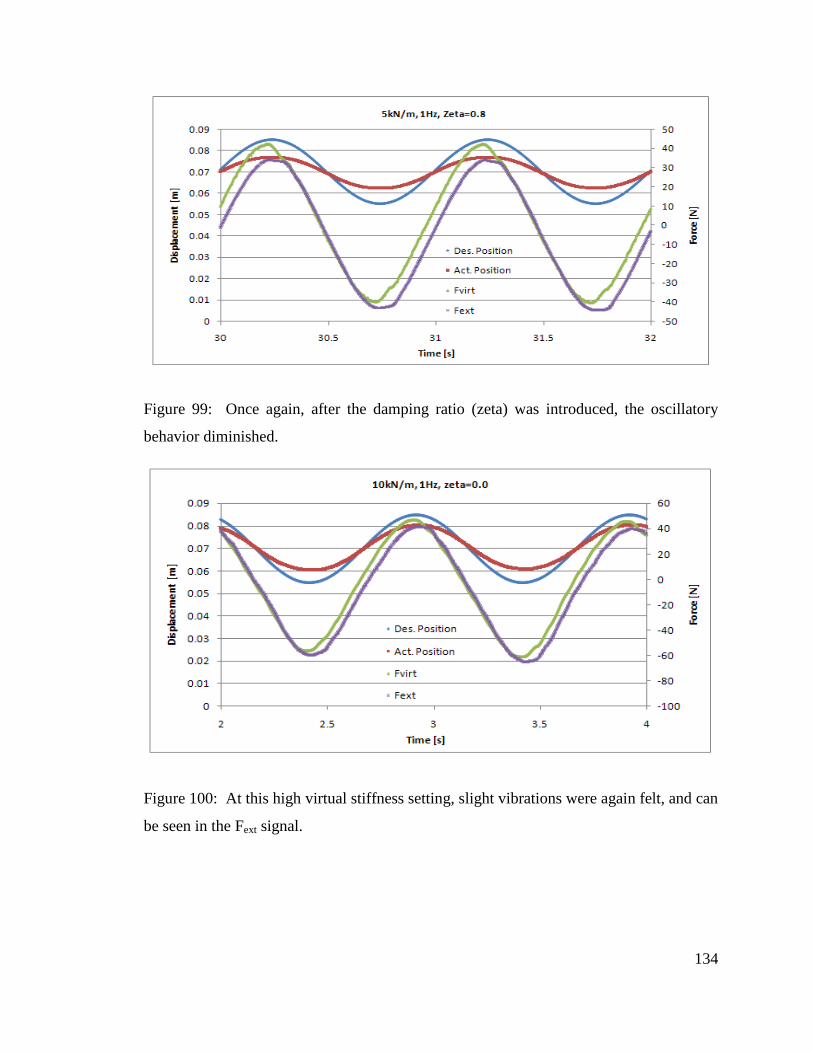
134
Figure 99: Once again, after the damping ratio (zeta) was introduced, the oscillatory
behavior diminished.
Figure 100: At this high virtual stiffness setting, slight vibrations were again felt, and can
be seen in the Fext signal.
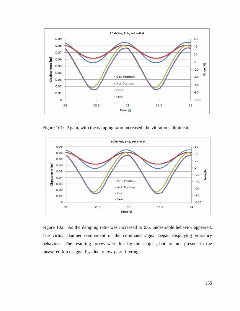
135
Figure 101: Again, with the damping ratio increased, the vibrations diminish.
Figure 102: As the damping ratio was increased to 0.6, undesirable behavior appeared.
The virtual damper component of the command signal began displaying vibratory
behavior. The resulting forces were felt by the subject, but are not present in the
measured force signal Fext due to low-pass filtering.
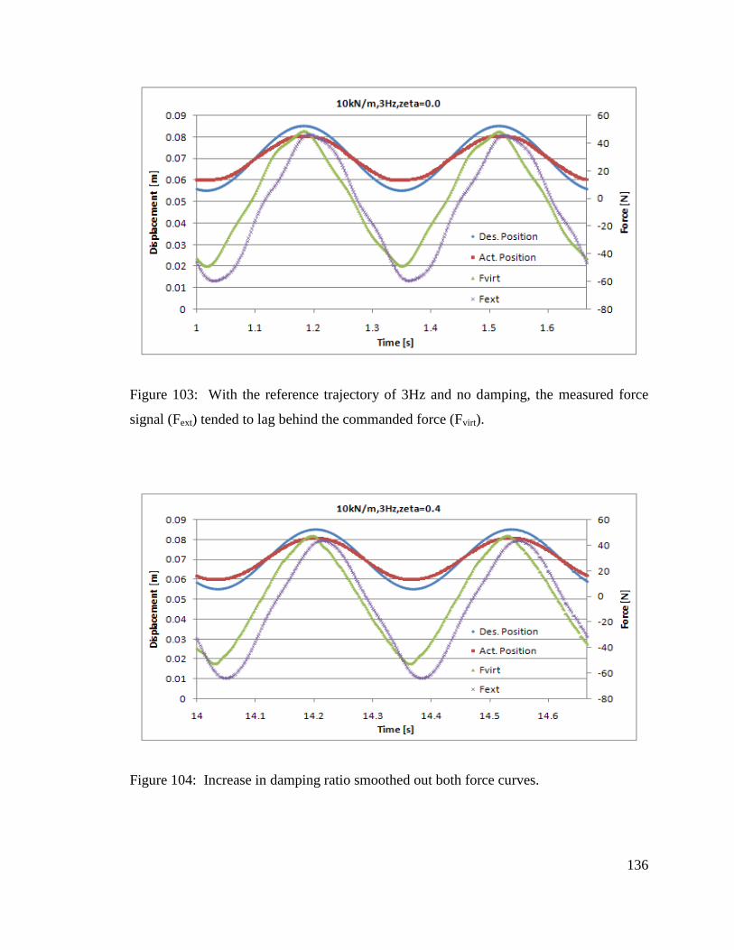
136
Figure 103: With the reference trajectory of 3Hz and no damping, the measured force
signal (Fext) tended to lag behind the commanded force (Fvirt).
Figure 104: Increase in damping ratio smoothed out both force curves.
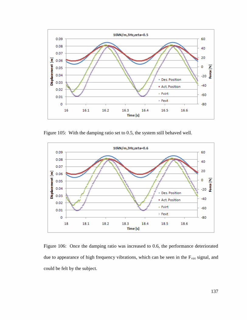
137
Figure 105: With the damping ratio set to 0.5, the system still behaved well.
Figure 106: Once the damping ratio was increased to 0.6, the performance deteriorated
due to appearance of high frequency vibrations, which can be seen in the Fvirt signal, and
could be felt by the subject.
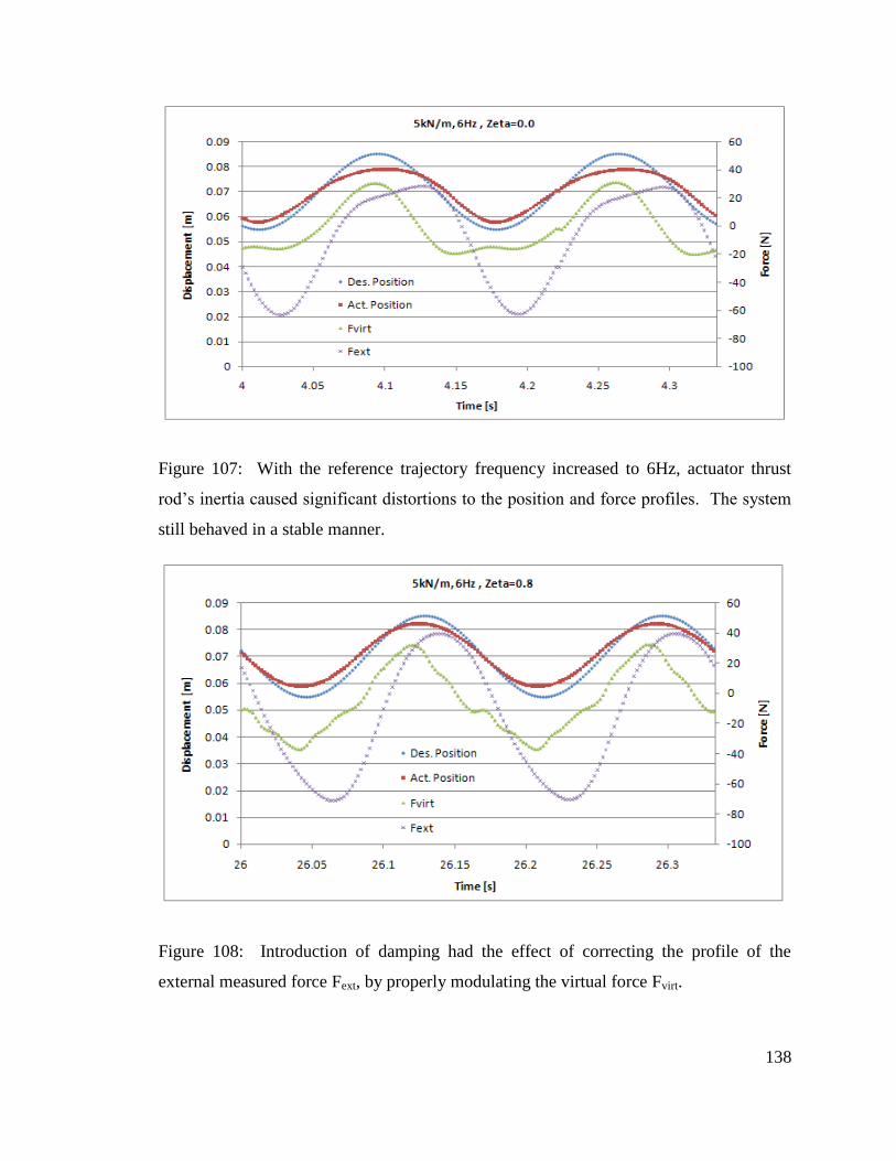
138
Figure 107: With the reference trajectory frequency increased to 6Hz, actuator thrust
rod’s inertia caused significant distortions to the position and force profiles. The system
still behaved in a stable manner.
Figure 108: Introduction of damping had the effect of correcting the profile of the
external measured force Fext, by properly modulating the virtual force Fvirt.
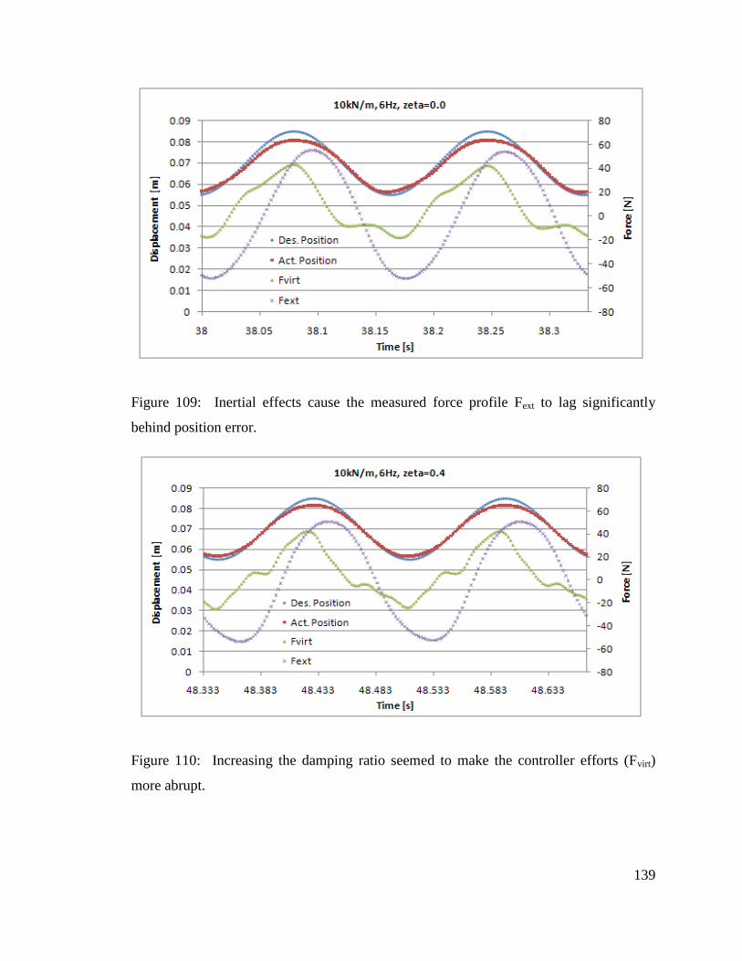
139
Figure 109: Inertial effects cause the measured force profile Fext to lag significantly
behind position error.
Figure 110: Increasing the damping ratio seemed to make the controller efforts (Fvirt)
more abrupt.
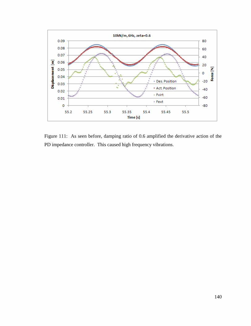
140
Figure 111: As seen before, damping ratio of 0.6 amplified the derivative action of the
PD impedance controller. This caused high frequency vibrations.
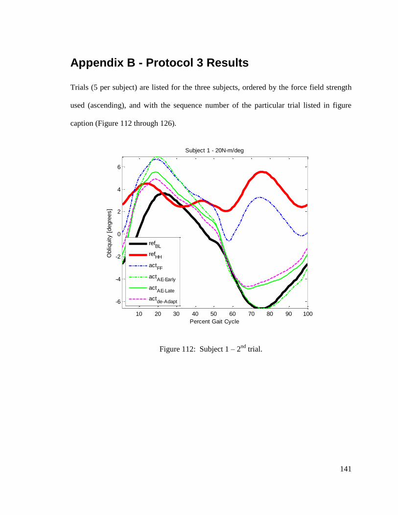
141
Appendix B - Protocol 3 Results
Trials (5 per subject) are listed for the three subjects, ordered by the force field strength
used (ascending), and with the sequence number of the particular trial listed in figure
caption (Figure 112 through 126).
Figure 112: Subject 1 – 2nd
trial.
10 20 30 40 50 60 70 80 90 100
-6
-4
-2
0
2
4
6
Percent Gait Cycle
Obliq
uity [
degre
es]
Subject 1 - 20N-m/deg
refBL
refHH
actFF
actAE-Early
actAE-Late
actde-Adapt
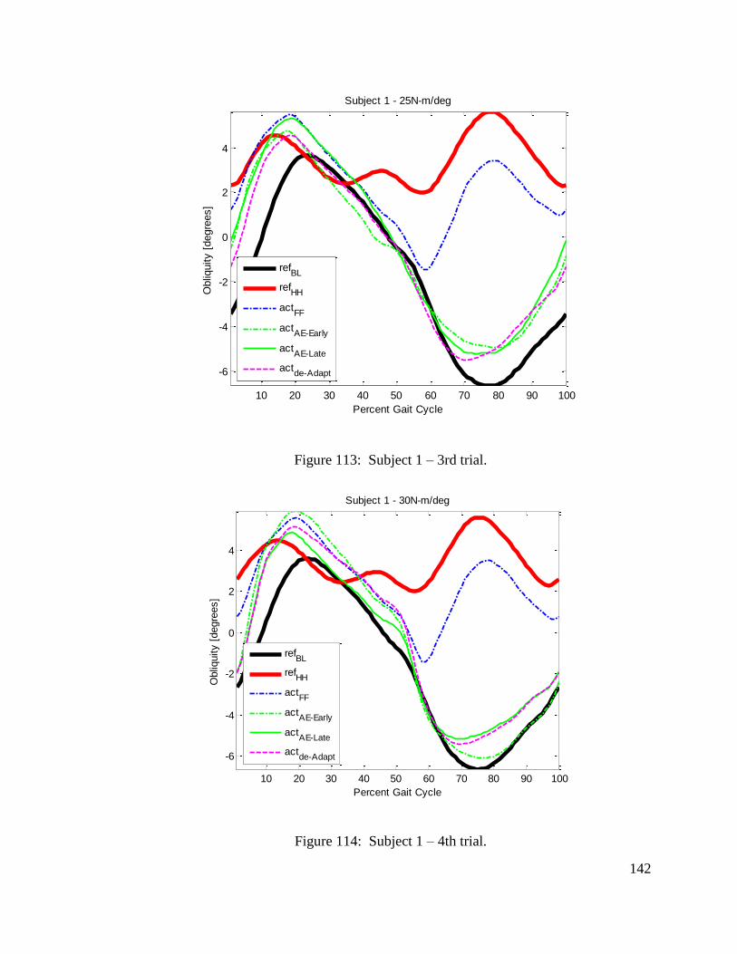
142
Figure 113: Subject 1 – 3rd trial.
Figure 114: Subject 1 – 4th trial.
10 20 30 40 50 60 70 80 90 100
-6
-4
-2
0
2
4
Percent Gait Cycle
Obliq
uity [
degre
es]
Subject 1 - 25N-m/deg
refBL
refHH
actFF
actAE-Early
actAE-Late
actde-Adapt
10 20 30 40 50 60 70 80 90 100
-6
-4
-2
0
2
4
Percent Gait Cycle
Obliq
uity [
degre
es]
Subject 1 - 30N-m/deg
refBL
refHH
actFF
actAE-Early
actAE-Late
actde-Adapt
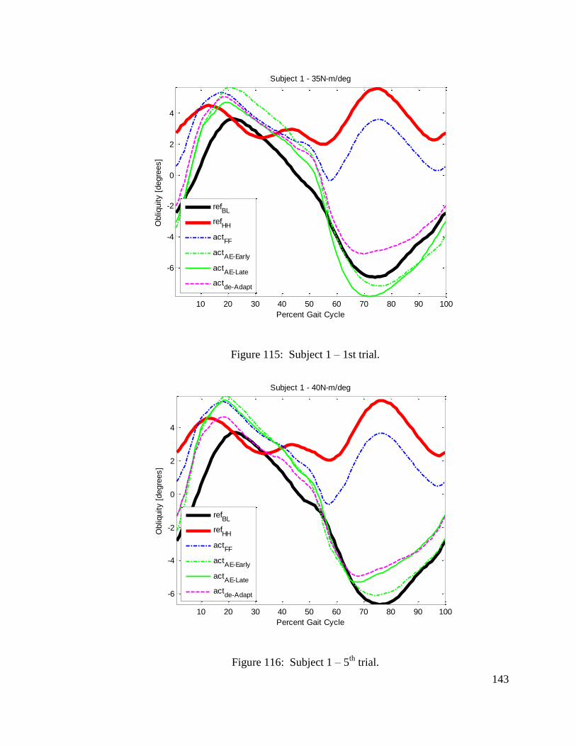
143
Figure 115: Subject 1 – 1st trial.
Figure 116: Subject 1 – 5th
trial.
10 20 30 40 50 60 70 80 90 100
-6
-4
-2
0
2
4
Percent Gait Cycle
Obliq
uity [
degre
es]
Subject 1 - 35N-m/deg
refBL
refHH
actFF
actAE-Early
actAE-Late
actde-Adapt
10 20 30 40 50 60 70 80 90 100
-6
-4
-2
0
2
4
Percent Gait Cycle
Obliq
uity [
degre
es]
Subject 1 - 40N-m/deg
refBL
refHH
actFF
actAE-Early
actAE-Late
actde-Adapt
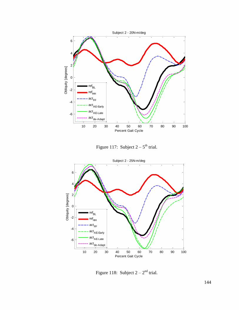
144
Figure 117: Subject 2 – 5th
trial.
Figure 118: Subject 2 – 2nd
trial.
10 20 30 40 50 60 70 80 90 100
-6
-4
-2
0
2
4
6
Percent Gait Cycle
Obliq
uity [
degre
es]
Subject 2 - 20N-m/deg
refBL
refHH
actFF
actAE-Early
actAE-Late
actde-Adapt
10 20 30 40 50 60 70 80 90 100
-6
-4
-2
0
2
4
6
Percent Gait Cycle
Obliq
uity [
degre
es]
Subject 2 - 25N-m/deg
refBL
refHH
actFF
actAE-Early
actAE-Late
actde-Adapt
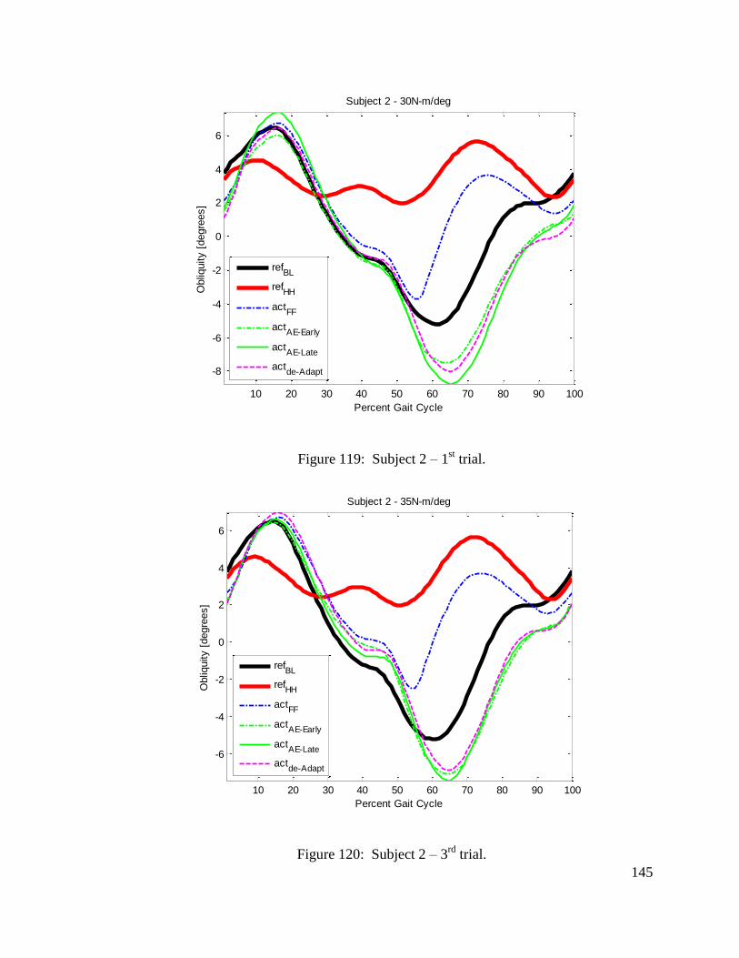
145
Figure 119: Subject 2 – 1st trial.
Figure 120: Subject 2 – 3rd
trial.
10 20 30 40 50 60 70 80 90 100
-8
-6
-4
-2
0
2
4
6
Percent Gait Cycle
Obliq
uity [
degre
es]
Subject 2 - 30N-m/deg
refBL
refHH
actFF
actAE-Early
actAE-Late
actde-Adapt
10 20 30 40 50 60 70 80 90 100
-6
-4
-2
0
2
4
6
Percent Gait Cycle
Obliq
uity [
degre
es]
Subject 2 - 35N-m/deg
refBL
refHH
actFF
actAE-Early
actAE-Late
actde-Adapt
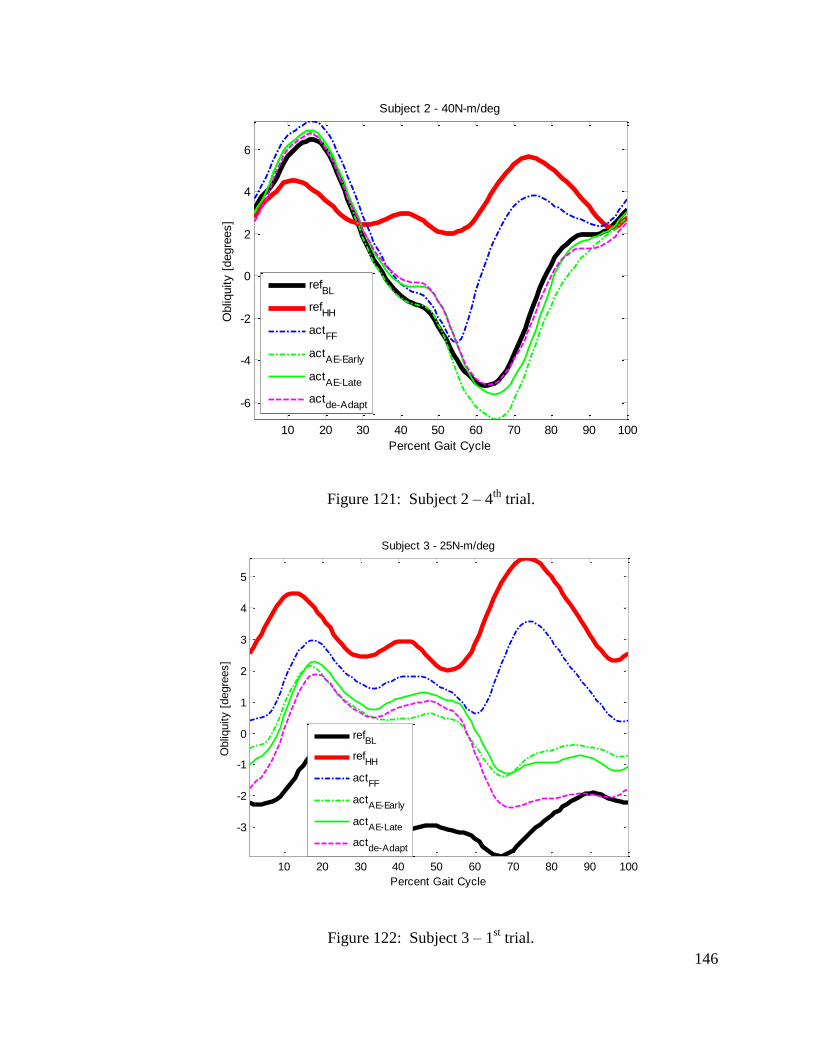
146
Figure 121: Subject 2 – 4th
trial.
Figure 122: Subject 3 – 1st trial.
10 20 30 40 50 60 70 80 90 100
-6
-4
-2
0
2
4
6
Percent Gait Cycle
Obliq
uity [
degre
es]
Subject 2 - 40N-m/deg
refBL
refHH
actFF
actAE-Early
actAE-Late
actde-Adapt
10 20 30 40 50 60 70 80 90 100
-3
-2
-1
0
1
2
3
4
5
Percent Gait Cycle
Obliq
uity [
degre
es]
Subject 3 - 25N-m/deg
refBL
refHH
actFF
actAE-Early
actAE-Late
actde-Adapt
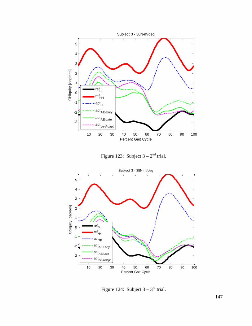
147
Figure 123: Subject 3 – 2nd
trial.
Figure 124: Subject 3 – 3rd
trial.
10 20 30 40 50 60 70 80 90 100
-3
-2
-1
0
1
2
3
4
5
Percent Gait Cycle
Obliq
uity [
degre
es]
Subject 3 - 30N-m/deg
refBL
refHH
actFF
actAE-Early
actAE-Late
actde-Adapt
10 20 30 40 50 60 70 80 90 100
-3
-2
-1
0
1
2
3
4
5
Percent Gait Cycle
Obliq
uity [
degre
es]
Subject 3 - 35N-m/deg
refBL
refHH
actFF
actAE-Early
actAE-Late
actde-Adapt
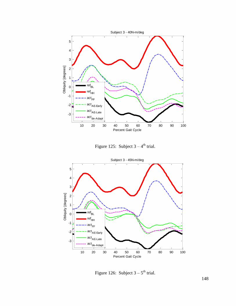
148
Figure 125: Subject 3 – 4th
trial.
Figure 126: Subject 3 – 5th
trial.
10 20 30 40 50 60 70 80 90 100
-3
-2
-1
0
1
2
3
4
5
Percent Gait Cycle
Obliq
uity [
degre
es]
Subject 3 - 40N-m/deg
refBL
refHH
actFF
actAE-Early
actAE-Late
actde-Adapt
10 20 30 40 50 60 70 80 90 100
-3
-2
-1
0
1
2
3
4
5
Percent Gait Cycle
Obliq
uity [
degre
es]
Subject 3 - 45N-m/deg
refBL
refHH
actFF
actAE-Early
actAE-Late
actde-Adapt
149
Appendix C - RGR Trainer 2DOF
Besides hip-hiking, another common secondary gait deviation occurring in the motion of
the pelvis is circumduction with exaggerated pelvic rotation, as shown in Figure 5.
Guiding pelvic rotation in order to affect this gait deviation requires the ability to
generate moments in the horizontal plane. The design of a 2 DOF RGR Trainer, which
can apply moments about pelvic obliquity and pelvic rotation, is presented.
Requirements
The device needs to be able to apply corrective moments to pelvic obliquity and pelvic
rotation, while allowing close to free translations in the horizontal plane. As is the case
with any impedance – controlled device for human interaction, the inertia of the device
should be kept to a minimum, in order to enhance the robot’s ability to display the
prescribed force fields. Considering the specific task at hand, it has been shown the
inertia of the robot should be less than that of the actuated body part [47]. The body
segment inertias can be found using equations in a NASA publication, based on the total
body weight (TBW) [48]. For a light subject, these inertias can be as low as 22.9kg in
vertical direction and 11.9kg in horizontal plane [49]. In that same work, the moment of
inertia of the pelvis for a female 1% by weight was found to be 0.1243kg-m2.
Static friction can cause the subject to lose balance. One study found that patients
couldn’t resist disturbances equal to 2% of their body weight [50]. Therefore, the
maximum allowable static friction force in the horizontal plane was found to be 8.3N
150
[49]. That same source found the maximum desirable stiffness applied onto the body to
be 4150N/m.
Actuation System Design Concepts
Concept 1
This concept design features two rigid links applying a moment at pelvic obliquity from
behind, and two links applying moment at pelvic obliquity from above the patient. In this
design concept the BWS system is integrated into the obliquity control parallelogram
mechanism, the two linkages need to be designed to fully support a subject weighing
111kg, which amounts to 545N. The forces exerted onto the component as a result of
moment application were calculated as well. Previous testing revealed that moments up
to 60N-m have significant impact on simulated hip-hiking. Therefore, an upper-bound
value of 100N-m was used for the moments applied to the pelvis. The moment-arm was
found based on the 1st percentile male’s hip width. The moment arm was found to be
264mm, and therefore the necessary force transmitted by a single link necessary to impart
the mentioned 100N-m moment was found to be 379N, putting the link in compression
and subject to failure due to buckling. For the purpose of clearing the subject’s upper
body, the link was designed to approximate an arc, with an offset of about 140mm. A
clearance of 165mm above the head of the 99th
percentile male was used. The link was
subjected to a static test in tension of 924N (body weight support and applied moment)
and a buckling test with a force of 379N (from moment application). The link’s change
in length due to compressive force (from moment application) amounted to just over
2mm. The result is a link which provides a safety factor of just above 2 for both modes,
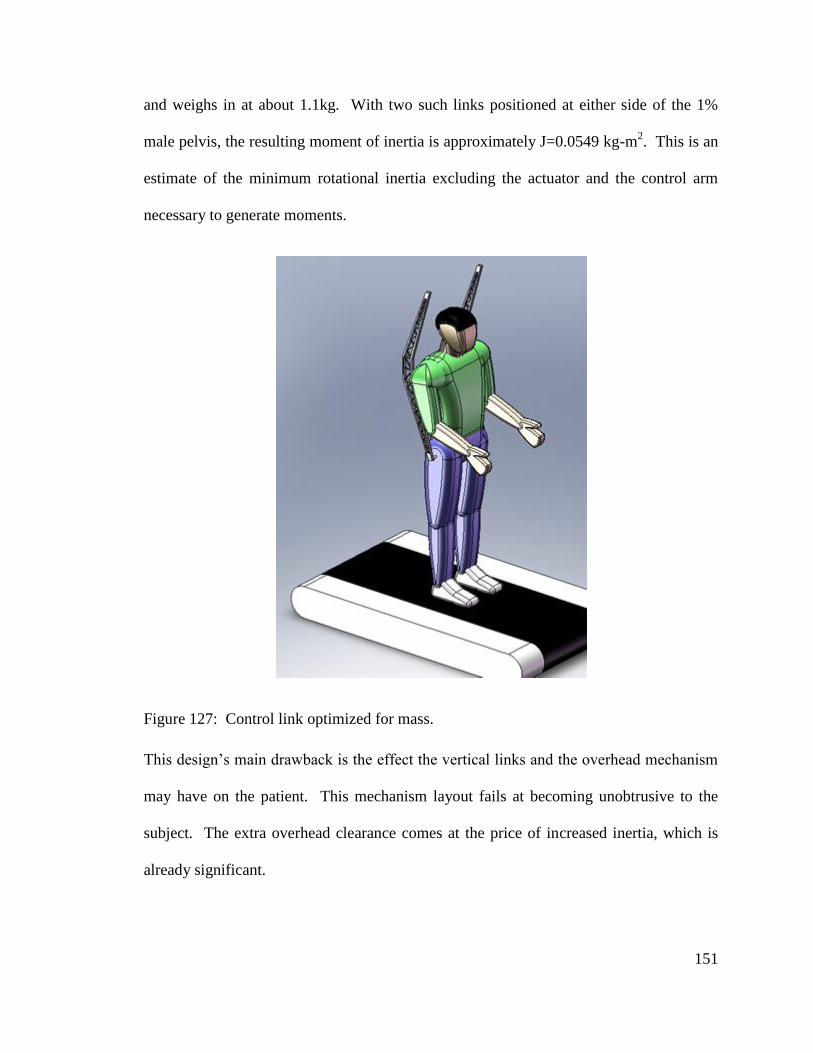
151
and weighs in at about 1.1kg. With two such links positioned at either side of the 1%
male pelvis, the resulting moment of inertia is approximately J=0.0549 kg-m2. This is an
estimate of the minimum rotational inertia excluding the actuator and the control arm
necessary to generate moments.
Figure 127: Control link optimized for mass.
This design’s main drawback is the effect the vertical links and the overhead mechanism
may have on the patient. This mechanism layout fails at becoming unobtrusive to the
subject. The extra overhead clearance comes at the price of increased inertia, which is
already significant.
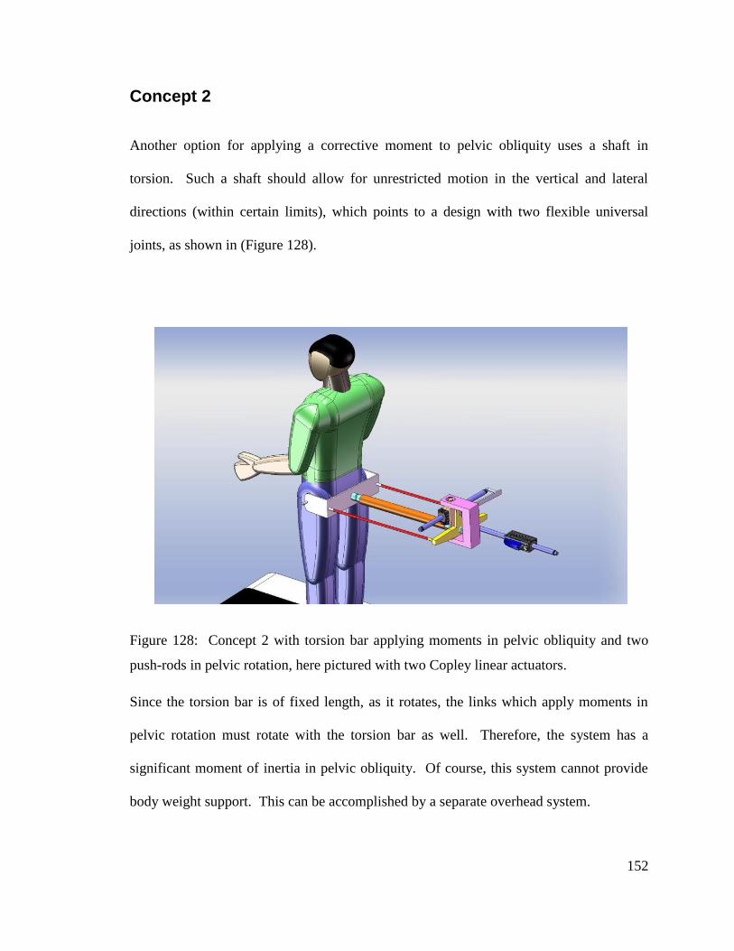
152
Concept 2
Another option for applying a corrective moment to pelvic obliquity uses a shaft in
torsion. Such a shaft should allow for unrestricted motion in the vertical and lateral
directions (within certain limits), which points to a design with two flexible universal
joints, as shown in (Figure 128).
Figure 128: Concept 2 with torsion bar applying moments in pelvic obliquity and two
push-rods in pelvic rotation, here pictured with two Copley linear actuators.
Since the torsion bar is of fixed length, as it rotates, the links which apply moments in
pelvic rotation must rotate with the torsion bar as well. Therefore, the system has a
significant moment of inertia in pelvic obliquity. Of course, this system cannot provide
body weight support. This can be accomplished by a separate overhead system.

153
Concept 3
This design consists of two parallel four-bar mechanisms, which support a cylindrical
joint for pelvic obliquity, and a semi-circle supported by bearings, which operates at the
pelvic rotation level with the remote center of rotation placed inside the subject’s body
(Figure 129). This design requires flexible transmission to deliver the driving moments
to the two rotational DOF’s. This reduces the mechanism’s inertia (actuators are
stationary), but the complexity of this design and necessity for high precision custom-
machined components make it a poor choice.
Figure 129: Constant-radius arc guided by bearings used to place the center of rotation
within the subject’s body.
Concept 4
The fourth concept features two triangular beams, which are constrained to rotate
together. This creates a structure fixed in rotation but free to translate, for application of
the moment to pelvic obliquity.
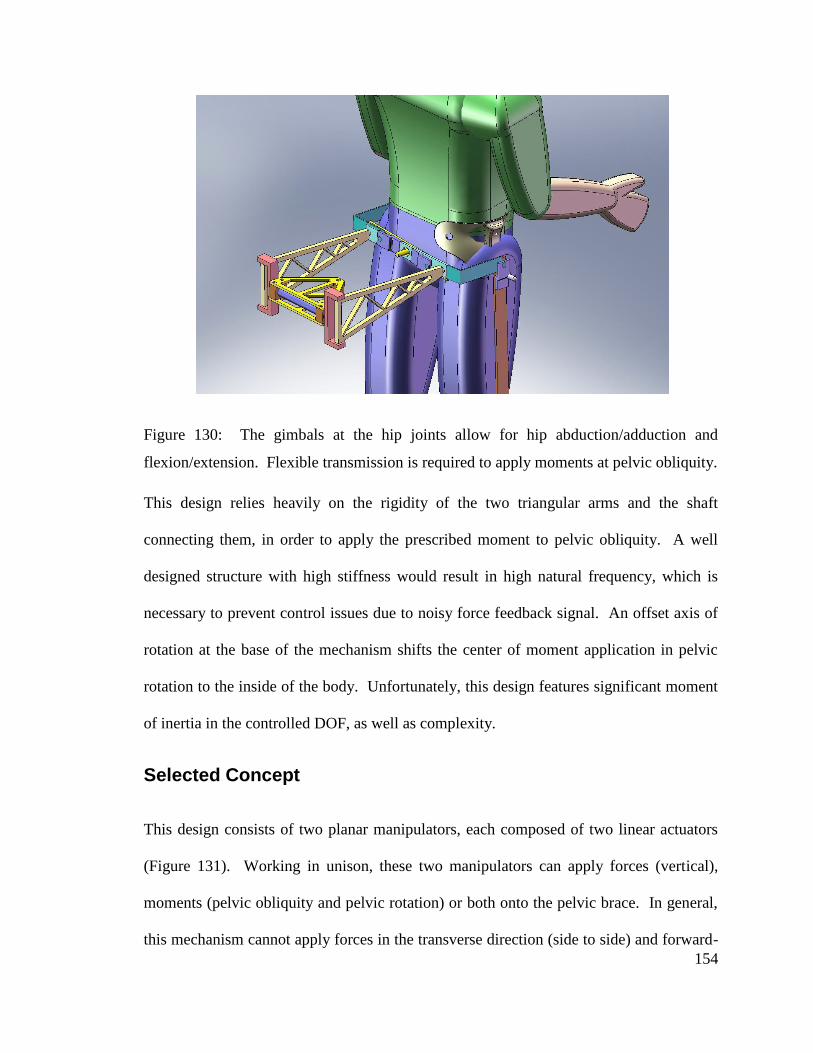
154
Figure 130: The gimbals at the hip joints allow for hip abduction/adduction and
flexion/extension. Flexible transmission is required to apply moments at pelvic obliquity.
This design relies heavily on the rigidity of the two triangular arms and the shaft
connecting them, in order to apply the prescribed moment to pelvic obliquity. A well
designed structure with high stiffness would result in high natural frequency, which is
necessary to prevent control issues due to noisy force feedback signal. An offset axis of
rotation at the base of the mechanism shifts the center of moment application in pelvic
rotation to the inside of the body. Unfortunately, this design features significant moment
of inertia in the controlled DOF, as well as complexity.
Selected Concept
This design consists of two planar manipulators, each composed of two linear actuators
(Figure 131). Working in unison, these two manipulators can apply forces (vertical),
moments (pelvic obliquity and pelvic rotation) or both onto the pelvic brace. In general,
this mechanism cannot apply forces in the transverse direction (side to side) and forward-
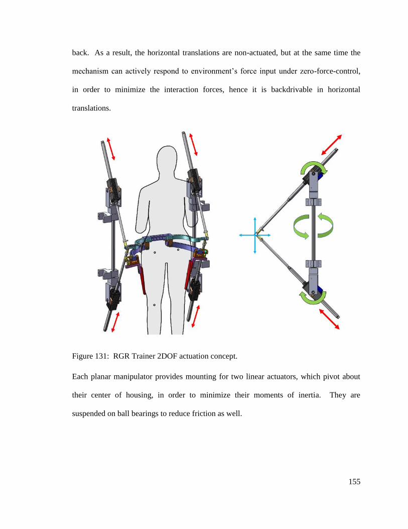
155
back. As a result, the horizontal translations are non-actuated, but at the same time the
mechanism can actively respond to environment’s force input under zero-force-control,
in order to minimize the interaction forces, hence it is backdrivable in horizontal
translations.
Figure 131: RGR Trainer 2DOF actuation concept.
Each planar manipulator provides mounting for two linear actuators, which pivot about
their center of housing, in order to minimize their moments of inertia. They are
suspended on ball bearings to reduce friction as well.
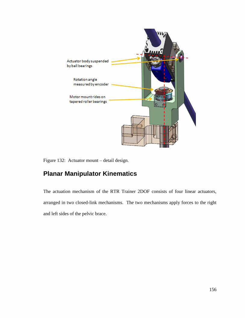
156
Figure 132: Actuator mount – detail design.
Planar Manipulator Kinematics
The actuation mechanism of the RTR Trainer 2DOF consists of four linear actuators,
arranged in two closed-link mechanisms. The two mechanisms apply forces to the right
and left sides of the pelvic brace.
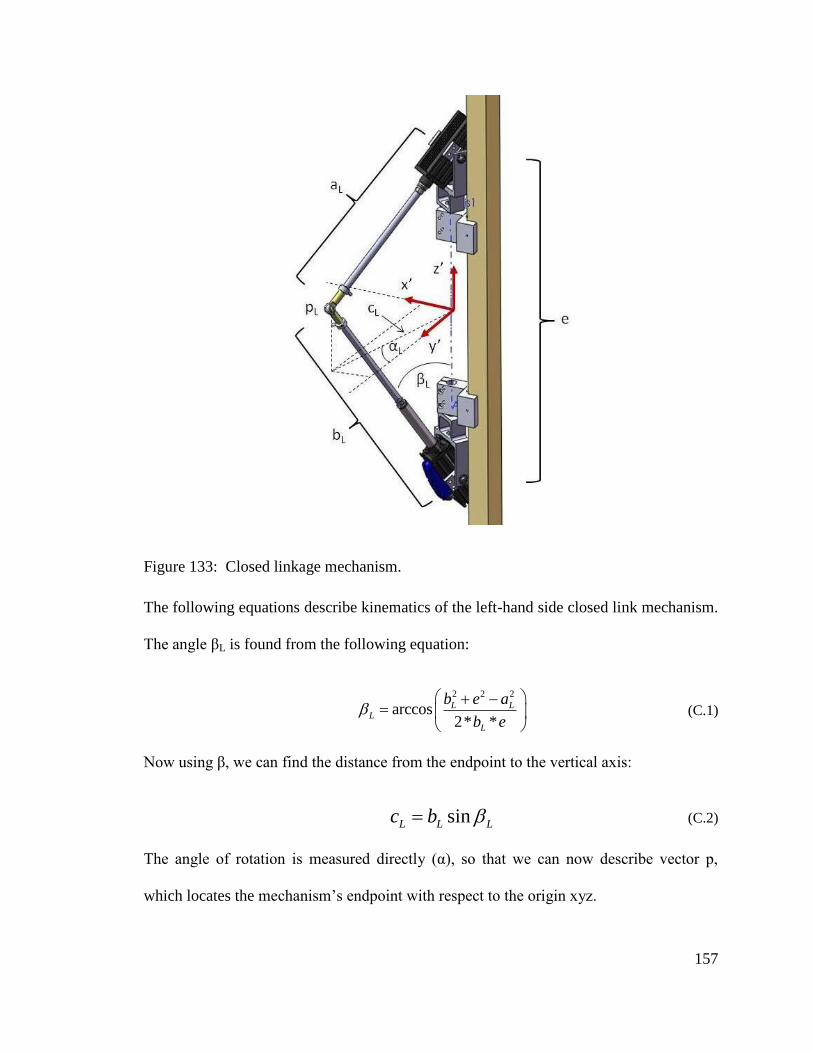
157
Figure 133: Closed linkage mechanism.
The following equations describe kinematics of the left-hand side closed link mechanism.
The angle βL is found from the following equation:
2 2 2
arccos2* *
L LL
L
b e a
b e
(C.1)
Now using β, we can find the distance from the endpoint to the vertical axis:
sinL L Lc b (C.2)
The angle of rotation is measured directly (α), so that we can now describe vector p,
which locates the mechanism’s endpoint with respect to the origin xyz.
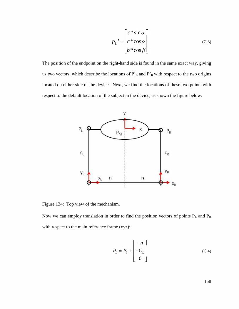
158
*sin
' *cos
*cos
L
c
p c
b
(C.3)
The position of the endpoint on the right-hand side is found in the same exact way, giving
us two vectors, which describe the locations of P’L and P’R with respect to the two origins
located on either side of the device. Next, we find the locations of these two points with
respect to the default location of the subject in the device, as shown the figure below:
Figure 134: Top view of the mechanism.
Now we can employ translation in order to find the position vectors of points PL and PR
with respect to the main reference frame (xyz):
'
0
L L L
n
P P C
(C.4)
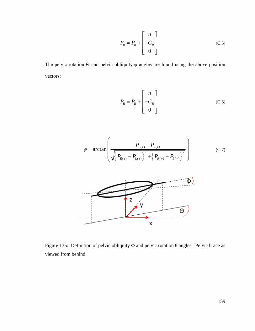
159
'
0
R R R
n
P P C
(C.5)
The pelvic rotation Θ and pelvic obliquity φ angles are found using the above position
vectors:
'
0
R R R
n
P P C
(C.6)
( ) ( )
2 2
( ) ( ) ( ) ( )
arctanL z R z
R z L z R y L y
P P
P P P P
(C.7)
Figure 135: Definition of pelvic obliquity Φ and pelvic rotation θ angles. Pelvic brace as
viewed from behind.
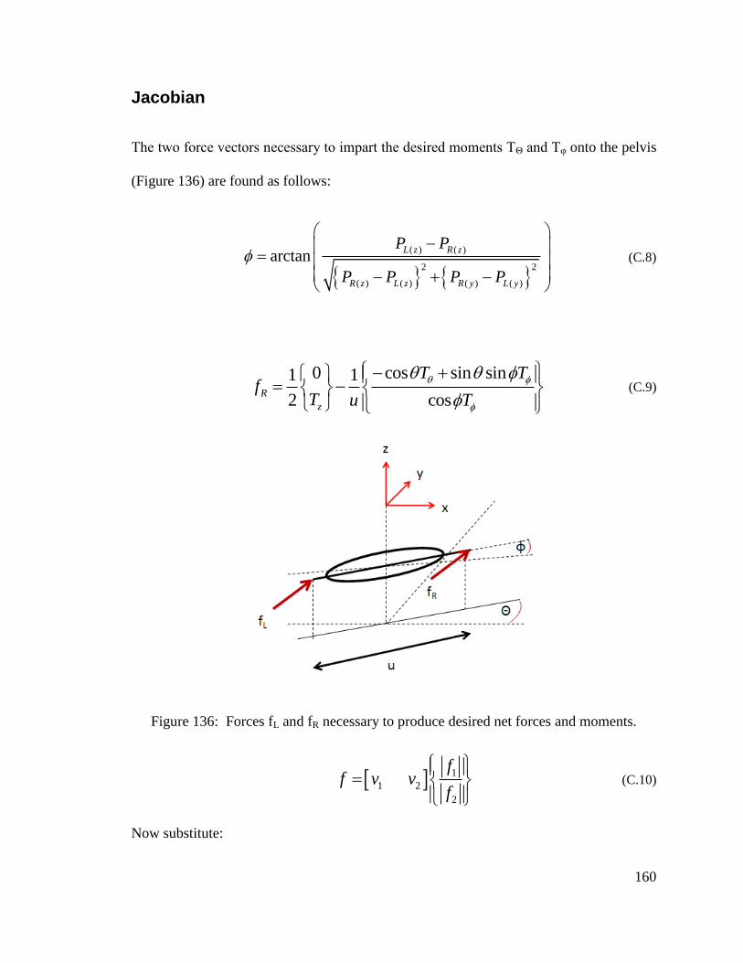
160
Jacobian
The two force vectors necessary to impart the desired moments ΤΘ and Τφ onto the pelvis
(Figure 136) are found as follows:
( ) ( )
2 2
( ) ( ) ( ) ( )
arctanL z R z
R z L z R y L y
P P
P P P P
(C.8)
cos sin sin01 1
2 cosR
z
T Tf
T u T
(C.9)
Figure 136: Forces fL and fR necessary to produce desired net forces and moments.
1
1 2
2
ff v v
f
(C.10)
Now substitute:
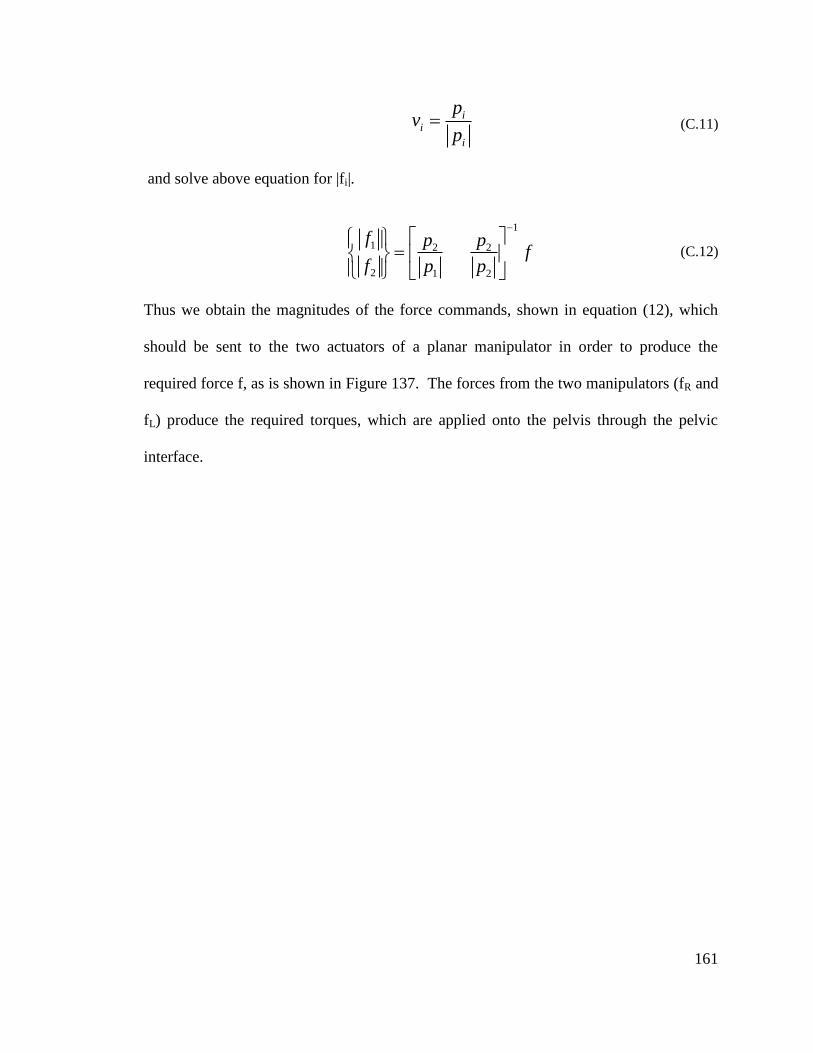
161
i
i
i
pv
p (C.11)
and solve above equation for |fi|.
1
1 2 2
2 1 2
f p pf
f p p
(C.12)
Thus we obtain the magnitudes of the force commands, shown in equation (12), which
should be sent to the two actuators of a planar manipulator in order to produce the
required force f, as is shown in Figure 137. The forces from the two manipulators (fR and
fL) produce the required torques, which are applied onto the pelvis through the pelvic
interface.
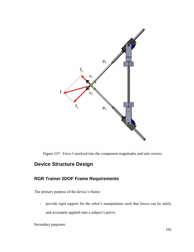
162
Figure 137: Force f resolved into the component magnitudes and unit vectors.
Device Structure Design
RGR Trainer 2DOF Frame Requirements
The primary purpose of the device’s frame:
- provide rigid support for the robot’s manipulators such that forces can be safely
and accurately applied onto a subject’s pelvis.
Secondary purposes:

163
- provide mounting for body weight support.
- provide support for upper body (handle bar).
Desirable features:
- unrestricted access for physical therapist from the side to either leg of the subject.
- ability to enter the device in wheel chair.
- easy machine adjustment for different height patients.
- simple, modular design for ease of installation on site.
- low price.
Frame Design
In order to fulfill the requirements set forth, a simple structure was designed, which
consists of rectangular cross section steel tubing, jointed by threaded fasteners (Figure
138 and Figure 139). The frame is wide enough for a wheel chair to enter the machine
from the rear. The handlebar design allows for height adjustment as well as fore-aft
adjustment. The robotic manipulators’ height is adjusted with a brake winch and cable –
pulley system, and is clamped into place with bolts, as shown in Figure 140. The handle
bar tilt is adjustable when quick release clamps are loosened, while adding to the
structural integrity of the frame when the clamps are tightened. Both adjustments can be
performed by just one person and without need for tools thanks to use of knobs, indexing
plunger and quick-release clamps (Figure 141 and Figure 142).
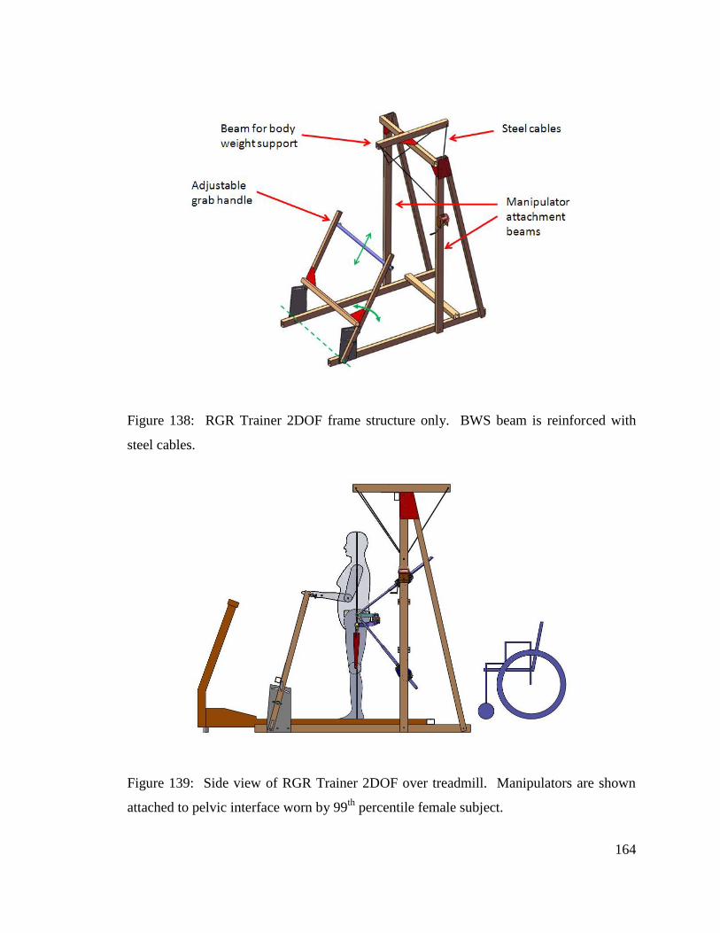
164
Figure 138: RGR Trainer 2DOF frame structure only. BWS beam is reinforced with
steel cables.
Figure 139: Side view of RGR Trainer 2DOF over treadmill. Manipulators are shown
attached to pelvic interface worn by 99th
percentile female subject.
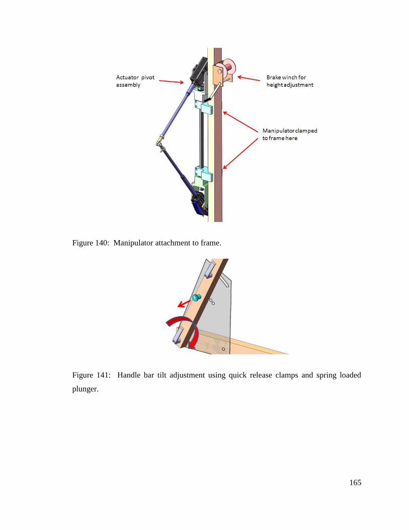
165
Figure 140: Manipulator attachment to frame.
Figure 141: Handle bar tilt adjustment using quick release clamps and spring loaded
plunger.
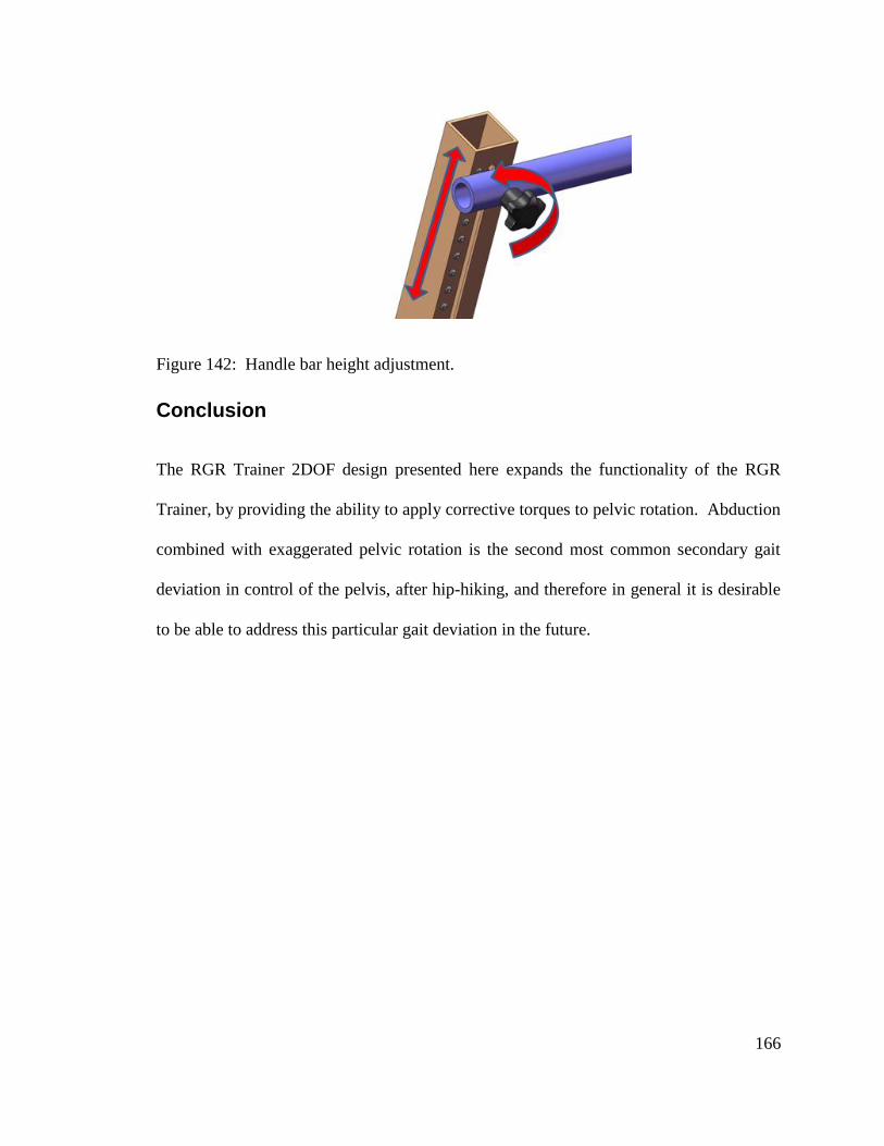
166
Figure 142: Handle bar height adjustment.
Conclusion
The RGR Trainer 2DOF design presented here expands the functionality of the RGR
Trainer, by providing the ability to apply corrective torques to pelvic rotation. Abduction
combined with exaggerated pelvic rotation is the second most common secondary gait
deviation in control of the pelvis, after hip-hiking, and therefore in general it is desirable
to be able to address this particular gait deviation in the future.
167
Bibliography
[1] V. L. Roger, A. S. Go, D. M. Lloyd-Jones, R. J. Adams, J. D. Berry, T. M.
Brown, M. R. Carnethon, S. Dai, G. de Simone, and E. S. Ford, "Executive
Summary: Heart Disease and Stroke Statistics—2011 Update," Circulation, vol.
123, pp. 459-463, 2011.
[2] J. M. Guralnik, A. Z. LaCroix, R. D. Abbott, L. F. Berkman, S. Satterfield, D. A.
Evans, and R. B. Wallace, "Maintaining mobility in late life. I. Demographic
characteristics and chronic conditions," Am J Epidemiol, vol. 137, pp. 845-57,
Apr 15 1993.
[3] J. M. Guralnik, L. Ferrucci, E. M. Simonsick, M. E. Salive, and R. B. Wallace,
"Lower-extremity function in persons over the age of 70 years as a predictor of
subsequent disability," N Engl J Med, vol. 332, pp. 556-61, Mar 2 1995.
[4] H. C. Chiu, J. Y. Chern, H. Y. Shi, S. H. Chen, and J. K. Chang, "Physical
functioning and health-related quality of life: before and after total hip
replacement," Kaohsiung J Med Sci, vol. 16, pp. 285-92, Jun 2000.
[5] E. Knutsson and C. Richards, "Different types of disturbed motor control in gait
of hemiparetic patients," Brain, vol. 102, pp. 405-30, Jun 1979.
[6] D. Aoyagi, W. E. Ichinose, S. J. Harkema, D. J. Reinkensmeyer, and J. E.
Bobrow, "A robot and control algorithm that can synchronously assist in
naturalistic motion during body-weight-supported gait training following
neurologic injury," IEEE Transactions on Neural Systems and Rehabilitation
Engineering, vol. 15, pp. 387-400, 2007.
[7] V. T. Inman, H. J. Ralston, F. Todd, and J. C. Lieberman, Human walking:
Williams & Wilkins Baltimore, 1981.
[8] D. A. Winter, Biomechanics and motor control of human movement, 1990.
[9] J. Perry, Gait analysis: normal and pathological function: SLACK incorporated,
1992.
[10] R. J. Nudo, E. J. Plautz, and S. B. Frost, "Role of adaptive plasticity in recovery
of function after damage to motor cortex," Muscle & nerve, vol. 24, 2001.
[11] E. Taub, G. Uswatte, and R. Pidikiti, "Constraint-induced movement therapy: a
new family of techniques with broad application to physical rehabilitation-a
clinical review," Journal of Rehabilitation Research and Development, vol. 36,
pp. 237-251, 1999.
[12] M. Visintin, H. Barbeau, N. Korner-Bitensky, and N. E. Mayo, "A new approach
to retrain gait in stroke patients through body weight support and treadmill
stimulation," vol. 29, ed: Am Heart Assoc, 1998, pp. 1122-1128.
[13] B. T. Volpe, H. I. Krebs, N. Hogan, L. Edelstein, C. Diels, and M. Aisen, "A
novel approach to stroke rehabilitation Robot-aided sensorimotor stimulation,"
Neurology, vol. 54, pp. 1938-1944, 2000.
[14] S. Hesse, C. Werner, D. Uhlenbrock, S. V. Frankenberg, A. Bardeleben, and B.
Brandl-Hesse, "An electromechanical gait trainer for restoration of gait in
hemiparetic stroke patients: preliminary results," Neurorehabilitation and neural
repair, vol. 15, p. 39, 2001.
168
[15] (2012, March 3). Body-Weight Supported Treadmill [Image]. Available:
http://www.beyond-therapy.org/files/image/auto-960-700-fit/b.jpg
[16] H. I. Krebs, N. Hogan, M. L. Aisen, and B. T. Volpe, "Robot-aided
neurorehabilitation," Rehabilitation Engineering, IEEE Transactions on, vol. 6,
pp. 75-87, 1998.
[17] J. F. Veneman, J. Menger, E. H. F. van Asseldonk, F. C. T. van der Helm, and H.
van der Kooij, "Fixating the pelvis in the horizontal plane affects gait
characteristics," Gait & Posture, 2007.
[18] (2009). Available:
http://srv6b.picturepark.com/UI/index.cfm?K=80&Action=getPDF&ID=879&La
ng=en
[19] J. F. Veneman, R. Kruidhof, E. E. G. Hekman, R. Ekkelenkamp, E. H. F. Van
Asseldonk, and H. Van der Kooij, "Design and evaluation of the LOPES
exoskeleton robot for interactive gait rehabilitation," IEEE Transactions on
Neural Systems and Rehabilitation Engineering, vol. 15, pp. 379-386, 2007.
[20] H. Schmidt, C. Werner, R. Bernhardt, S. Hesse, and J. Krüger, "Gait rehabilitation
machines based on programmable footplates," Journal of NeuroEngineering and
Rehabilitation, vol. 4, p. 2, 2007.
[21] S. Hussein, H. Schmidt, M. Volkmar, J. Kruger, and S. Hesse, "Muscle activation
of stroke patients during stair climbing in robot assisted gait training," in
Biomedical Robotics and Biomechatronics, 2008. BioRob 2008. 2nd IEEE RAS &
EMBS International Conference on, 2008, pp. 875-880.
[22] D. Aoyagi, W. Ichinose, D. Reinkensmeyer, and J. Bobrow, "Human step
rehabilitation using a robot attached to the pelvis," 2004.
[23] J. L. Emken, J. H. Wynne, S. J. Harkema, and D. J. Reinkensmeyer, "A robotic
device for manipulating human stepping," Robotics, IEEE Transactions on, vol.
22, pp. 185-189, 2006.
[24] H. Krebs, B. Volpe, M. Aisen, and N. Hogan, "Increasing productivity and quality
of care: robot-aided neuro-rehabilitation," Journal of Rehabilitation Research and
Development, vol. 37, pp. 639-652, 2000.
[25] R. Riener, L. Lunenburger, S. Jezernik, M. Anderschitz, G. Colombo, and V.
Dietz, "Patient-cooperative strategies for robot-aided treadmill training: first
experimental results," IEEE Transactions on Neural Systems and Rehabilitation
Engineering, vol. 13, pp. 380-394, 2005.
[26] N. Hogan and S. P. Buerger, "Stable, high-force, low-impedance robotic actuators
for human-interactive machines," 2005.
[27] G. Colombo and A. Hocoma, "Physiological Treadmill Training with the 8-DOF
Rehabilitation Robot LOKOMAT," presented at the Jahrestagung der deutschen
Gesellschaft für biomedizinische Technik (Conference of the German Society of
Biomedical Engineering), Nürnberg, 2005.
[28] A. Zoss, H. Kazerooni, and A. Chu, "On the mechanical design of the Berkeley
lower extremity exoskeleton (BLEEX)," 2005, pp. 3465-3472.
[29] H. Dreyfuss, The measure of man: human factors in design: Whitney Library of
Design, 1967.
[30] E. Churchill, L. Laubach, J. McConville, and I. Tebbetts, "Anthropometric source
book. Volume 1: Anthropometry for designers," 1978.
169
[31] N. Hogan, "Stable execution of contact tasks using impedance control," in
Robotics and Automation. Proceedings. 1987 IEEE International Conference on,
1987, pp. 1047-1054.
[32] D. W. Meer and S. M. Rock, "Coupled-system stability of flexible-object
impedance control," in Robotics and Automation, 1995. Proceedings., 1995 IEEE
International Conference on, 1995, pp. 1839-1845 vol.2.
[33] S. Lennon, "The Bobath concept: a critical review of the theoretical assumptions
that guide physiotherapy practice in stroke rehabilitation," Physical therapy
reviews, vol. 1, pp. 35-45, 1996.
[34] J. M. Belda-Lois, S. Mena-del Horno, I. Bermejo-Bosch, J. C. Moreno, J. L. Pons,
D. Farina, M. Iosa, M. Molinari, F. Tamburella, and A. Ramos, "Journal of
NeuroEngineering and Rehabilitation," Journal of NeuroEngineering and
Rehabilitation, vol. 8, p. 66.
[35] S. Rossignol, R. Dubuc, and J. P. Gossard, "Dynamic sensorimotor interactions in
locomotion," Physiological reviews, vol. 86, pp. 89-154, 2006.
[36] J. Norton, "Changing our thinking about walking," The Journal of Physiology,
vol. 588, p. 4341, 2010.
[37] R. Shadmehr and F. A. Mussa-Ivaldi, "Adaptive representation of dynamics
during learning of a motor task," The Journal of neuroscience, vol. 14, pp. 3208-
3224, 1994.
[38] A. J. Bastian, "Understanding sensorimotor adaptation and learning for
rehabilitation," Current opinion in neurology, vol. 21, p. 628, 2008.
[39] S. M. Morton and A. J. Bastian, "Cerebellar contributions to locomotor
adaptations during splitbelt treadmill walking," The Journal of neuroscience, vol.
26, pp. 9107-9116, 2006.
[40] I. Cajigas, M. T. Goldsmith, A. Duschau-Wicke, R. Riener, M. Smith, E. Brown,
and P. Bonato, "Assessment of lower extremity motor adaptation via an extension
of the Force Field Adaptation Paradigm," 2010, pp. 4522-4525.
[41] S. H. Kim, S. K. Banala, E. A. Brackbill, S. K. Agrawal, V. Krishnamoorthy, and
J. P. Scholz, "Robot-assisted modifications of gait in healthy individuals,"
Experimental brain research, vol. 202, pp. 809-824, 2010.
[42] E. van Asseldonk, B. Koopman, and H. van der Kooij, "Locomotor adaptation
and retention to gradual and sudden dynamic perturbations," 2011, pp. 1-5.
[43] D. S. Reisman, R. Wityk, K. Silver, and A. J. Bastian, "Locomotor adaptation on
a split-belt treadmill can improve walking symmetry post-stroke," Brain, vol. 130,
p. 1861, 2007.
[44] T. Cruz, M. Lewek, and Y. Dhaher, "Biomechanical impairments and gait
adaptations post-stroke: Multi-factorial associations," Journal of Biomechanics,
vol. 42, pp. 1673-1677, 2009.
[45] S. K. Banala, S. K. Agrawal, and J. P. Scholz, "Active Leg Exoskeleton (ALEX)
for gait rehabilitation of motor-impaired patients," 2007, pp. 401-407.
[46] E. V. L. Vasudevan and A. J. Bastian, "Split-belt treadmill adaptation shows
different functional networks for fast and slow human walking," Journal of
Neurophysiology, vol. 103, p. 183.
[47] A. Sharon and J. Charnnarong, "The design of an intelligent machine for upper-
limb physical therapy," 1991.

170
[48] Anthropometric source book volume I: Anthropometry for Designers (NASA RP-
1024), 1978.
[49] H. I. Krebs and M. M. H. Roberts, "A robot for gait rehabilitation," 2004.
[50] S. G. B. Kirker, J. R. Jenner, D. S. Simpson, and A. M. Wing, "Changing patterns
of postural hip muscle activity during recovery from stroke," Clinical
rehabilitation, vol. 14, p. 618, 2000.
![Journal of NeuroEngineering and Rehabilitation BioMed Central...nized Gait Trainer [17,18], Lokomat® [19,20] and PAM, POGO and ARTHuR [21] are all examples of robotic devices that](https://img.pdfslide.us/doc/110x75/61085ab8b97ec57e51016c07/journal-of-neuroengineering-and-rehabilitation-biomed-central-nized-gait-trainer.jpg)