The Robotic Assembly Line Design (RALD) problem: Model andcase studies with practical extensions

Adalberto Sato Michelsa , Thiago Cantos Lopesa , Celso Gustavo Stall Sikoraa , LeandroMagataoa∗

a: Graduate Program in Electrical and Computer Engineering (CPGEI)

Federal University of Technology - Parana (UTFPR), Curitiba, Brazil, 80230-901

Abstract

Spot welding assembly lines are widely present in the automotive manufacturing industry. The

procedure of building the vehicle’s body employs several robots equipped with spot welding tools.

These robots and tools are a quite costly initial investment, requiring an efficient and conscious

line design that meets product demands and minimises implementation expense at the same time.

In this paper, the Robotic Assembly Line Design (RALD) problem is proposed and studied based

on practical characteristics from an automotive company located in Brazil. A Mixed-Integer Liner

Programming (MILP) formulation is developed allowing: (i) station paralleling, (ii) equipment se-

lection, and (iii) multiples robots per workstation. The mathematical model aims at minimising the

total cost at the desired production rate, which involves robots, tools and facilities. The proposed

model considers dead time during a cycle, space constraints, task assignment restrictions, and par-

allelism possibilities. Dead time is an unproductive and fixed work-piece handling time included in

the capacitated transporter robots’ movement time. Computational experiments were performed

in order to evidence the parameters’ influence over the optimal line design solution. In addition,

practical case studies were conducted with parameters collected from a real-world robotic welding

assembly line located on the outskirts of Curitiba-PR (Brazil), reaching optimality. Compared

to the strictly serial lines, the model led to great advantages by allowing parallel stations in the

production system, making it possible to evaluate an expected trade-off between the production

rate and the total cost; reductions of several hundred thousand dollars on the production layout

cost can be achieved by the company, as indicated by the studied cases.

Keywords: Robotic assembly line design; Station paralleling; Equipment selection; Dead time;

Mixed-integer linear programming

c© 2019. This manuscript version is made available under the CC-BY-NC-ND 4.0 license

http://creativecommons.org/licenses/by-nc-nd/4.0/

Computers & Industrial Engineering, Volume 120, June 2018, Pages 320-333

DOI: 10.1016/j.cie.2018.04.010

∗Corresponding authorEmail address: magatao@utfpr.edu.br (Leandro Magataoa)

Accepted manuscript published by Computers & Industrial Engineering July 31, 2019

1. Introduction

Production systems used in the automotive industry are frequently based on assembly lines for

regular operation. This variety of configuration has given rise to traditional assembly line balancing

problems (ALBP), vastly approached in the literature. However, most part of the research focuses

on achieving the best assignment of tasks among several stations arranged in a serial line considering

many restricting assumptions, which not always describe and solve more realistic problems (Battaıa

& Dolgui, 2013).

Although the literature on ALBP is quite extensive, a gap between the practical and theoretical

cases still exists (Becker & Scholl, 2006; Boysen et al., 2008; Battaıa & Dolgui, 2013). In real-world

lines, flexible assembly systems are adopted and must be properly designed in order to reach the

desired production rate at the minimum cost, which includes facilities, programmable robots and

equipment selection. Therefore, the global decisions made by the company necessitate and depend

on the optimal solution for the line layout, which comes along with the balancing objective in an

integrated problem.

Researches concerning ALBP are also strongly related to the automotive industry, mainly to

the final stage assembly. Notwithstanding, the arrangement of body-shop stages also consists

of assembly or manufacturing lines that can be treated by ALBP formulations (Lopes et al.,

2017b). The body-in-white stage transforms sheets of metal into the vehicle’s body by using

welding procedures. This stage is composed of welding assembly lines that are usually highly

automated (Michalos et al., 2010). Welding procedures might present several spot welding tasks

with similar characteristics. Formulations can take advantage of the high multiplicity of welding

tasks and treat them as a group of similar tasks. Therefore, these similar tasks can be gathered

together into a single task with a given number of copies of the same task, since their processing

times are virtually identical (Sikora et al., 2017b). Moreover, welding tasks are found in the body-

shop stage and these tasks fall into three main categories: geometry, stud, and finishing tasks.

Geometry welding tasks assemble the metal sheet pieces together, stud welding tasks add screws

on the metal sheets’ surface, and finishing welding tasks are used to reinforce the vehicle’s structure.

Geometry and finishing tasks can be performed with identical tools, but a different tool is required

in order to execute stud tasks.

According to Baybars (1986), these differences in describing realistic features divide the clas-

sification of ALBPs in two and make the problems fall into one of these categories: the Simple

Assembly Line Balancing Problem (SALBP), or the General Assembly Line Balancing Problem

(GALBP). In SALBPs, the system is only restricted by precedence relations and cycle time con-

straints, whereas GALBPs regard further specification, such as task incompatibility, space con-

straints, station paralleling, multiple and capable workers, equipment selection, or unproductive

time, among others. An extensive review on SALBP is done by Scholl & Becker (2006), the same

is done for GALBP by Becker & Scholl (2006), and a more recent survey on ALBPs is done by

Battaıa & Dolgui (2013).

The solution methods for ALBPs are separated into exact and approximate approaches. The

2

first one seeks the optimality, whilst the other includes heuristics and meta-heuristics procedures,

which are intended to produce comparatively good results in a reduced computing time. Surveys on

exact and heuristic methods are found in Scholl (1999); Scholl & Becker (2006) and Becker & Scholl

(2006) for SALBP and GALBP, respectively. For meta-heuristics, some common improvement

procedures applied in ALBPs are: tabu search (Suwannarongsri & Puangdownreong, 2008), ant

colony optimisation (Sabuncuoglu et al., 2009), simulated annealing (Cakir et al., 2011), and genetic

algorithms (Sikora et al., 2016).

Thus far, we can declare that GALBPs are generalisations of SALBPs, since they consider

relaxing one or any combination of the SALBP stated assumptions. However, GALBPs still omit

some designing sub-problems, such as selecting the equipment depending on the set of candidate

solutions for each manufacturing operation, costs of dimensioning the production area, and the

layout itself (Baybars, 1986). For instance, Bukchin & Rubinovitz (2003) show a case study in

which different tasks can only be performed by different equipment, and distributing limited units

of these tools is necessary. At the same time, parallel stations are required due to long task

durations higher than the demanded cycle time, changing the line’s configuration. Amen (2006)

assumes each station to have a pre-specified investment. In automotive industry, these concepts

can be extended to welding gun selection for particular tasks and capital costs of robots in an

automated assembly line. Whenever these fixed and variable costs (facilities, technology, operation)

are taken into account, we have a further generalisation of the GALBP, namely Assembly Line

Design Problem (ALDP) (Baybars, 1986). For exact methods, heuristics and meta-heuristics that

deal with the ALDP, Rekiek et al. (2002) provide a comprehensive review. Nonetheless, as assembly

line balancing and design problems are intimately linked, this nomenclature boundary is not always

observed, and some design problems are named “balancing problems” by their authors. This fact

is notably attested by the further explored literature.

Many of these ALBP extensions are explored individually. For instance, Rubinovitz & Bukchin

(1991, 1993) introduced the Robotic Assembly Line Balancing (RALB) problem, and a method

based on branch and bound algorithm that aimed to minimise the number of workstations (type-

I), while allocating robots into a (balanced) robotic assembly line. This model, however, does not

analyse how workers (or robots, in the said case) behave in the production system when multiple

robots, equipment selection, and parallel stations are considered. Cycle time minimisation variants

(type-II) of the RALB problem were introduced by Levitin et al. (2006) and Gao et al. (2009).

More recently, a multi-objective version of the type-II RALB considering set-up and robot costs

minimisation as secondary objectives has been presented (Yoosefelahi et al., 2012).

Applicable variations of the GALBP might be incorporated in the robotic models. Multiple

workers could be assigned to the same station (Fattahi & Roshani, 2011; Yazgan et al., 2011),

some workers might be able to perform tasks in more than one station and, hence, they would

have to move between them (Sikora et al., 2017a), inclusion of workers with different capabilities

or tools may be studied as in Araujo et al. (2015), that use disabled workers in the line, and

ergonomic factors can be considered to decide workstation positioning on the line (Baykasoglu

3

et al., 2017). Multiple product design alternatives are investigated to influence balancing decisions:

mixed-model assembly lines can be evaluated by several objective functions and require products

to be sequenced, Lopes et al. (2017a) analyse and compare them considering buffer positions (if

any) and product sequences as parameters, whereas Oesterle et al. (2017) incorporate such product

design alternatives into balancing and equipment selection decisions and test their formulation with

numerous multi-objective algorithms. Furthermore, tasks cannot always be assigned to any station

(Deckro, 1989), some set of specific tasks frequently must be allocated either at the same station

(inclusion constraints), or are incompatible and must be placed at different stations (exclusion

constraints) (Scholl et al., 2010). Task incompatibility occurs when a pair of tasks cannot be

assigned to the same station due to practical characteristics of the operation and, therefore, the

precedence diagram is not sufficient to describe the precedence relations between tasks (Park et al.,

1997). This particularity is also found in body-shop stages of automotive industries and is further

explained in Section 2, by Figure 6. Other incompatibility problems might also happen due to

position or accessibility problems (Essafi et al., 2010), fixed machinery (Scholl et al., 2010), among

others.

In parallel stations, each station has its effective cycle time multiplied by its parallelism degree,

allowing more time for operations. Therefore, another particularity applied on line design problem

is the inclusion of parallelism as an option for better balancing solutions when there are tasks with

longer duration times than the desirable cycle time or the system’s efficiency requires improvement.

Lusa (2008) supplies a survey of parallelism applications in ALBPs, summarising the state of the

art for the combined problem. Station and line paralleling extensions are approached by several

authors, Askin & Zhou (1997) use a heuristic procedure for the mixed-model line with parallel

stations, while Bard (1989) presents a dynamic programming algorithm which takes into account

equipment and task costs, as well as unproductive time between cycles (dead time), which is

mostly affiliated with transportation time between stations. The transportation time of work-

pieces is attached to the movement of a conveyor or the time a robot takes to move a work-piece in

(set-up) and out (tear-down) of a station, this usually is a fixed and unproductive handling time.

Some authors examine fixed and variable line configuration design costs in the planning stage,

with decisions connected to the balancing problem, characterising such studies as ALDPs: Bukchin

& Rubinovitz (2003), Ege et al. (2009), Dolgui et al. (2012), Yoosefelahi et al. (2012), and Tuncel

& Topaloglu (2013) research potential advantages and drawbacks in station paralleling, including

equipment selection, labour costs, positional constraints, and task assignment restrictions. Parallel

stations require more space, hence additional constraints limiting the parallelism degree should also

be considered. Both Kim et al. (2000) and Guney & Ahiska (2014) consider a two-sided assembly

line, the first one is dealt with using a genetic algorithms, whereas the other is solved by mixed-

integer programming and is applied on an automotive industry in order to decide the optimal

automation level. For industrial robotic lines, these designing decisions ought to be combined with

cost minimisation procedures as to determine the production system layout. Amen (2000, 2006)

provide a survey on heuristic procedures, model formulations, and methods to solve cost-oriented

4

problems. In order represent and solve practical problems, several herein mentioned real-world

aspects must be taken into consideration simultaneously.

In this work, we develop a mathematical model that minimises the designing cost of an assembly

line considering several realistic aspects found in the automotive industry: (i) robots, (ii) their

space and accessibility constraints, (iii) equipment selection for each of them, (iv) task assignment

restrictions (incompatibility and special precedence), (v) parallel stations, and (vi) unproductive

time due to work-pieces movement between stations (dead time). The combination of these realistic

aspects are not present in previous ALDP models, thus a new model is herein proposed and

solved. The paper is organised as follows. In Section 2, the practical extensions of the problem are

explained in order to introduce the Robotic Assembly Line Design (RALD) problem. Section 3

presents the Mixed-Integer Linear Programming (MILP) model developed for solving the general

case of the problem and the practical case study. Section 4 analyses the case studies and the effects

on the production system layout once the line designing cost ratios and unproductive times are

altered. Lastly, in Section 5, concluding remarks are summarised and future research directions

are suggested.

2. Problem statement

The Robotic Assembly Line Design (RALD) problem is proposed and studied in this paper. We

aim at the optimisation of an assembly line’s layout. The decisions concern the length of the line

along with the number and type of robots assigned to the line. Tasks requiring different types of

tools are balanced within the line, while the transport system and parallel stations are also layout

decisions of the problem. In order to ease the understanding of the problem’s features, Figure 1

will be used as a visual support.

We consider that a robotic assembly line is composed of platform stations and transporter

robots to displace work-pieces between these platforms, as illustrated by Figure 1. Multiple robots

may be assigned to each platform station. By defining each transporter or platform as a station,

and assuming the line starts and finishes with a transporter robot, the configuration results in a

line with an odd number of stations in an alternating pattern of platform-fixed and transporter

robots. More examples can be found in Figures 7, 8, 9, and 10 of Section 4.

In this example of Figure 1, the first transporter robot is on a track-motion device (S1) and has

a welding tool placed on its side. The second station (S2) is a parallel platform station composed

of two cells with four robots each. The third station (S3) is also paralleled, contains two cells of

transporter robots, and each robot has a stud tool placed on its side. The forth station (S4) has

only one cell and holds three robots. The fifth and last station (S5) is a single transporter cell

without any task performing tool placed sideways.

The line allows parallelism of both platform and transporter stations. However, when a non-

paralleled transporter is adjacent to a paralleled platform station, a track-motion device is required.

Notice that the track-motion device applied on station S1 is necessary for its transporter robot to

reach both cells of station S2.

5

IN

Second station: a platform station composedof two cells with four robots each.

S1 S2 S3 S4

OUT

S5

Figure 1: Example of elements in the proposed RALD problem are shown: parallelism in platform

and transporter stations, multiple platform and transporter robots holding different tools or placed

sideways, and transporter robots on track-motions.

The robots are assigned to platform or transporter stations composed of one cell (single sta-

tions) or two identical parallel cells (double stations). The transportation of work-pieces between

the stations is done by manipulator robots. Commonly, these movement times (dead times) are

neglected in the problem formulation, a simplification that may lead to unreliable solutions. An

advantage of using robotic arms as transporters is that they can also perform tasks on work-pieces

during a cycle time between their loading and unloading operations.

Platform robots holding welding tools are dedicated exclusively to perform assembly tasks, while

transporter robots are mainly used for moving products in and out of the stations, but they also

can use the remaining time of their cycle to perform tasks as long as they have a static tool placed

on the line’s sideways. This condition can be observed in stations S1 and S3 of Figure 1. These

transporter robots that are capable of performing tasks are named capacitated transporter robots.

Such robots are under the effect of an increased time penalisation on task time duration, since they

take longer to perform the same tasks robots in platform stations do. This increment in the task

time duration happens because, whereas in platform stations the work-pieces are steady for the

robot to access the spot welding points, in transporter stations the robots have to manipulate the

entire work-piece in order to make the points accessible to the tool. For many industry segments,

tools are usually lighter and smaller than the produced work-pieces.

Figure 2 is a picture of platform robots assembling a work-piece (highlighted in blue) by per-

forming welding tasks. The welding guns (highlighted in yellow) are held by the robots and the

product stays fixed in the station. As the movement between welding spots is small, so is the

processing time of the tasks.

Figure 3, on the other hand, is a picture of a transporter robot that uses a static welding tool.

6

Figure 2: Platform robots performing welding tasks at the same time on the same blue work-piece.

The yellow welding guns that each robot holds are highlighted in the picture.

The yellow welding gun, in this case, is placed in the line’s sideways and the robot moves the entire

blue work-piece in order to make the welding spots accessible to the welding gun and perform the

required tasks in a diminished rate. Platforms and capacitated transporter robots can be very

similar. In our example, the same robot model can be employed both in platform and transport

stations, the difference lays on the tools attached to them.

Figure 3: Transporter robot holding the entire work-piece and manipulating it to the welding gun

placed on the line’s sideways. The work-piece that the robot holds and the static yellow welding

gun are highlighted in the picture.

7

Generally, robotic arms are not long enough to reach both sides of a parallel station (at least

for large work-pieces, such as vehicle parts, for instance). These transporter robots might be

placed on track-motion devices in order to allow them to reach adjacent paralleled stations and

avoid unnecessary transporter station paralleling. Although the device allows more reach to the

robot, an additional unproductive time penalty tied to the track-motion device movement should

be accounted on the robot’s cycle time. Figure 4 portrays a transporter robot placed on a track-

motion device set to unload a platform station. The arrow placed on the track-motion device

shows the movement that it permits. Figure 1 depicts this alternated pattern between platform

and transport stations, as well as equipment disposition and several other characteristics of the

RALD problem from a simplified top side view. Parallel station advantages and spot welding

processes are explained separately in this section.

Figure 4: Transporter robot on a track-motion device unloading a work-piece from a parallel

platform station.

Firstly formulated by Rubinovitz & Bukchin (1991) and later dealt with a genetic algorithm

(GA) by Levitin et al. (2006), the robotic assembly line balancing (RALB) problem is incorporated

into the problem we have at hand. Some general assumptions can be kept from their work since

the balancing core characteristic for the single product problem is present in our formulation:

1. The cycle time to meet the demand is known.

2. The assembly tasks precedence diagram is known.

3. There are no precedence relations within a station.

4. The duration of a task is deterministic and cannot be subdivided.

5. Robots and equipment are available at any quantity.

The specific problem has some differences. They are highlighted in bold in the following as-

sumptions:

6. The duration of a task depends on which robot and tool is assigned to perform it.

8

7. Parallel stations are allowed.

8. For the general case, any task can be performed at any station when the precedence relations

and equipment requirements are attended.

9. Multiple robots may be assigned to each station on the line not considering task scheduling

within stations.

10. Transportation time for loading (set-up) and unloading (tear-down) are considered. There-

fore, dead time is considered (Bard, 1989).

11. The goal is to minimise design cost, both robots and equipment have their prices as

parameters.

These highlighted aspects distinguish the classical RALB problem from our RALD problem:

lines are not strictly serial, i.e. either platform or transporter workstations can be doubled (see

second and third stations in Figure 1) in order to improve efficiency at a reduced cost, unproductive

transportation time is considered in the mathematical formulation, and multiple robots holding

different tools are allowed at the same station (see second and forth stations in Figure 1).

Station paralleling might lead to some advantages over single lines. The cycle time increase at

the doubled station is one of them, mainly when the dead time is considered, since the relative im-

portance of movement times (set-up and tear-down) is reduced. This effect is depicted in Figure 5,

showing how parallel stations affect the line efficiency positively.

In Figure 5, cycle times of two serial and parallel stations are presented on a schematic diagram.

In the first case (S1 and S2), for a given cycle time of 48 time units, set-up and tear-down times

of 12 time units each, the processing time (useful time) represents only 50% of the cycle time

(24 time units represented by the larger block placed on its top) and set-up and tear-down (dead

time) the other 50% (12 time units each represented by the smaller blocks). When the station is

doubled, one work-piece should be delivered per station every two cycles, in an alternated fashion.

Each copy of it (P1 and P2) benefits from paralleling and increases its useful time to 75% (72

time units) of their doubled cycle time (96 time units). Therefore, there is more available time

to be dedicated to task performing activities, an improvement of 50% in the useful time. The

work-piece handling time (dead time) is the same for both configurations when loading (set-up)

or unloading (tear-down) stations. However, the relative importance of this manipulation time is

reduced because such work-piece handling process is conducted fewer times. The efficiency gain

depends on which tasks were allocated to the serial stations and which could be allocated to an

equivalent paralleled one.

Moreover, secondary advantages of paralleling stations are the improvement in productivity as

a consequence of better balancing (Boysen et al., 2007) and the reduction on failure sensitivity,

albeit the reduced production rate (Rekiek et al., 2002). These reasons make parallel stations a

potentially profitable feature to be allowed into the line for practical applications. Nonetheless,

there are some drawbacks in the practical use: doubled stations might require greater investments

on equipment and higher operational costs. Not only the costs represent a trade-off, also larger

space is required for the double stations, robots and equipment, which forces limits on the number

9

Serial Station

(S1)

Serial Station

(S2)

Parallel Station (P1)

Parallel Station (P2)

OUTIN

IN OUT Set-Up Time

Processing Time

Tear-Down Time

Time unit[TU]

12 36 48 60 84 960

Time unit[TU]

12 84 960

Figure 5: Schematic comparative between serial and parallel stations. The benefits of paralleling

a station increase as the dead time represents a higher proportion of the cycle time.

of robots per workstation and paralleling degree.

Even disregarding the aforementioned drawbacks, paralleling stations indefinitely is not always

possible depending on which tasks one is performing. For instance, the automotive manufacture

widely uses the Resistance Spot Welding (RSW) technique in order to perform welding tasks in

the body-in-white stage. This process unites metal sheets by using welding guns, which, in turn,

require accessibility on both sides of the piece and, therefore, multiple types of this tool may be

necessary as the welding steps proceed. In addition, metal sheet joining tasks must respect geomet-

ric tolerances, demanding external actuators to bind the metal sheets to be united in the proper

position. Such tasks are called geometry tasks. Due to precision conditions, these geometry tasks

must be performed at platform stations and the stations in which they are processed must not

be paralleled for quality control.

Furthermore, the RSW technique is also used for reinforcement welding and screw adding

points, namely finishing and stud tasks, respectively. Differently from geometry tasks, these ones

do not require actuators to assure geometric tolerances and, theoretically, there are no precedence

relations among any welding point. However, these spot welding points might become inaccessible

after geometry tasks are performed, since the newly added sheets block the access of inner layers.

These blockages can be seem as station-wise accessibility windows that can be represented as a

special precedence diagram (see Figure A.11 on page 30). Moreover, this welding assembly line

property creates an incompatibility restriction between piece joining tasks (geometry tasks) and

reinforcement tasks (finishing and stud tasks): all reinforcement tasks must be completed a station

before any successor geometry task is allocated, since piece joining must be the first operation

10

performed at a station and reinforcement tasks would not be accessible after joining parts.

Figure 6 exemplifies why task incompatibility exists. Two car parts have to be joined, which

requires geometry tasks. This operation must be the first to be performed at a station due to the

use of external actuators. Yet once it is completed, some reinforcing welding procedures (finishing

and stud tasks on the base pieces) become inaccessible for the robots in the assembled set. The

region that becomes inaccessible is denoted by the area in which an overlap is verified between

the base pieces. For instance, consider a spot welding point P that requires a finishing task and

belongs to the first base piece, as illustrated by Figure 6. As stated before, welding procedures

need access to both sides of the metal sheet to be performed. If the required finishing task is not

performed on P before joining the base pieces, this point would be inaccessible afterwards, due to

an inner layer blockage.

Figure 6: Two car parts are assembled by platform robots performing geometry tasks. After the

assemblage, the welding point P becomes inaccessible to further reinforcing welding procedures,

therefore creating an incompatibility restriction between specific tasks.

The assemblage of succeeding metal sheets is the only reason for the precedence relations

between tasks. Since incompatible tasks must be performed at different stations (and before being

inaccessible), it is possible to use multiples robots not considering the task scheduling within a

station by the automotive industry. This is further discussed in Section 3.

Therefore, after the presented considerations, the configuration of an entire robotic line can be

defined, conceiving the Robotic Assembly Line Design (RALD) Problem: how many robots per

platform and transporter stations should be installed, how many tools of each type to use, which

tasks are assigned to each robot considering equipment availability, and which stations would need

to be paralleled in order to meet the demand at minimum cost. These decisions must all be made

simultaneously to assure the optimal solution. The summary of elements in the optimisation model

is shown in Figure 1 and are hereafter detailed as:

• Parallelism possibilities: both platform and transporter stations are allowed to be single

or double stations;

• Platform and transporter robots: multiple robots per platform cell are allowed, and

both platform and transporter robots are capable of performing tasks as long as they have a

tool assigned to them;

11

• Equipment selection: different types of tools may be assigned to platform and transporter

robots, even at the same station;

• Track-motion device possibility: transporter robots might be placed on track-motion

devices, this feature is required for single transporters adjacent to double platforms due to

the size of the products to be assembled.

Ultimately, if one knows the productivity rate to meet the demand (desired cycle time of the

line), the best solution will be the one that accomplishes this need and satisfies the precedence and

space constraints at the lowest cost.

3. Robotic assembly line design (RALD) model

This section contains a Mixed-Integer Linear Programming (MILP) formulation for the Robotic

Assembly Line Design (RALD) considering the problem definition and its characteristics described

in Section 2. In order to ease the model’s understanding, a concept based on the initial letter orien-

tation will be employed for the parameters, sets, and variables definition as follows: all parameters

and sets are written with an initial capital letter, an initial “b” indicates a binary variable (domain

in {0, 1}) and an initial “v” indicates a non-negative continuous (domain in R+) or integer variable

(domain in Z+).

Table 1 contains the applied terminology, describing the parameters and the sets used in the

formulation. The parameters are empirically collected based on industrial conditions, such as

available physical space and suppliers’ prices. Note that the maximum number of stations (NS)

must always be an odd number due to: (i) work-piece initial handling and final manipulation

out of the line, and (ii) the transporter-platform sequential stations characteristic of the problem,

which make transporter stations to be indexed with odd numbers and platform stations with even

numbers. Figure 1 on page 6 illustrates a line with an odd number of stations planned in an

alternated pattern. The variables are detailed in Table 2, they are created by the model depending

on the sets.

The problem’s objective function is to minimise the purchase cost of the line. As it is described

in Expression 1, the line’s cost is composed of the cost of the platform and transporter robots

along with their tools, platforms, and track-motions.

Minimise:∑

(s,e)∈SEs∈Sp

RPCoste · vTNRs,e

︸ ︷︷ ︸platform robots’ cost

+∑

(s,e)∈SEs∈St

RTCoste · vTNRs,e

︸ ︷︷ ︸transporter robots’ cost

+

+ PCost ·∑s∈Sp

(bSos + bSds)︸ ︷︷ ︸platform cost

+TMCost ·∑s∈St

bTMs︸ ︷︷ ︸track-motion cost

(1)

The layout planning depends on balancing tasks among workstations. For each workstation,

the number of robots, station paralleling, and the presence of track-motion devices delimit the

12

Table 1: Terminology: names of parameters and sets, their meaning, and [dimensional units].

Parameter Meaning

NT Number of tasks

NS Maximum number of stations (an odd number, NS ≥ 3)

Nmax Maximum number of robots per cell

CT Cycle time [time units]

DT Dead time [time units]

TM Time penalisation for track-motion [time units]

Dt,e Duration [time units] of task t performed by equipment e

Nt Number of copies of task t

PCost Platform cost [$]

TMCost Track-motion cost [$]

RTCoste Transporter robot cost [$] holding equipment e

RPCoste Platform robot cost [$] holding equipment e

Set Meaning

T Set of tasks t

S Set of stations s

St Set of transporter stations s, odd stations in S

Sp Set of platform stations s, even stations in S

TS Set of feasible Task-Station elements

SE Set of feasible Station-Equipment elements

TSE Set of feasible Task-Station-Equipment elements

Prec Set of precedence relations between two tasks ti and tj : (ti, tj)

SS Set of tasks that require single stations

Inc Set of incompatible tasks ti and tj : (ti, tj)

available time for operations to be performed. The inequalities for the balancing core of the model

(Inequalities 2 to 5) are based on the formulation for the high dimensionality (Integer) SALBP,

presented by Sikora et al. (2017b) and applied on real-world instances from an automotive body

welding assembly line. In this alternative formulation, decision variables for each existent type

of task are defined and replicas of a task are treated in a single integer variable. Therefore,

instead of creating binary variables to determine whether a task is assigned to a station or not,

the integer based formulation relies on integer variables that decide how many copies of each type

of task are assigned to each station. Assembly lines with high multiplicity of identical tasks (e.g.

resistance spot welding tasks) may be modelled using fewer variables than traditional binary based

formulations.

Equation 2 is the occurrence restriction. While binary based formulations allocate every task

individually, Equation 2 states that the sum of all allocations of task t assigned to stations must

be equal to its number of copies Nt. The precedence restriction is given by Inequality 3. Each task

13

Table 2: Terminology: definition of the model’s variables.

Variable Set Domain Meaning

vTdt,s,e (t, s, e) ∈ TSE Z+

Task designation: set to the number of copies of task t assigned at

station s using equipment e

bTet,s t ∈ T, s ∈ S {0, 1} Task ending: set to 1 if all the copies of task t are finished up to station s

bTot,s (t, s) ∈ TS {0, 1} Task occurrence: set to 1 if any copy of task t is performed at station s

bSos s ∈ S {0, 1} Station opened: set to 1 if station s needs to be used

bSds s ∈ S {0, 1} Station doubled: set to 1 if station s needs to be parallel

bTMs s ∈ St {0, 1}Transporter station with track-motion: set to 1 if the robot in

transporter station s is on a track-motion device

vNRs,e (s, e) ∈ SE Z+ Number of robots per cell in the station s holding equipment e

vTNRs,e (s, e) ∈ SE Z+ Total number of robots per station s holding equipment e

vUTs,e (s, e) ∈ SE R+ Useful time at the station s using equipment e [time units]

can only be assigned to a station (by task designation variable vTd) if all of its predecessors have

already been completed (measured by task ending variable bTe) in or before a station s. The link

between vTd and bTe variables for the same task is given by Inequalities 4 and 5. Inequality 4

assures bTe can only assume 1 if all Nt copies of the task are already performed up to station s,

hence allowing followers to be assigned. Complementary, Inequality 5 forces bTe = 1 when the

task is finished. This last restriction can be seen as a cut. Although it is not necessarily mandatory

to formulate the problem correctly, it can help to tighten the formulation.∑(t,s,e)∈TSE

vTdt,s,e = Nt ∀ t ∈ T (2)

bTeti,s ·Ntj ≥ vTdtj ,s,e ∀ (ti, tj) ∈ Prec, (tj , s, e) ∈ TSE (3)

bTet,s ≤∑

(t,sa,e)∈TSEsa≤s

vTdt,sa,eNt

∀ t ∈ T, s ∈ S (4)

bTet,s + Nt − 1 ≥∑

(t,sa,e)∈TSEsa≤s

vTdt,sa,e ∀ t ∈ T, s ∈ S (5)

Bukchin & Rubinovitz (2003) state that there is a diminishing return in paralleling stations.

The first station in parallel improves the efficiency, whereas the contribution of additional parallel

stations is quite small. Moreover, having many parallel station is only needed due to long task

times, which do not happen in spot welding assembly lines (Sikora et al., 2017b). Besides, the

cost of adding another copy of a robotic cell and the transporter accessibility to the stations would

result in unaffordable or infeasible production layouts due to the size of vehicles. Therefore, we

only consider possibilities of single or double stations.

The variable vUT is responsible for the measurement of the useful time used to perform tasks,

and is calculated by summing the performed tasks (Equation 6). The available time depends on

14

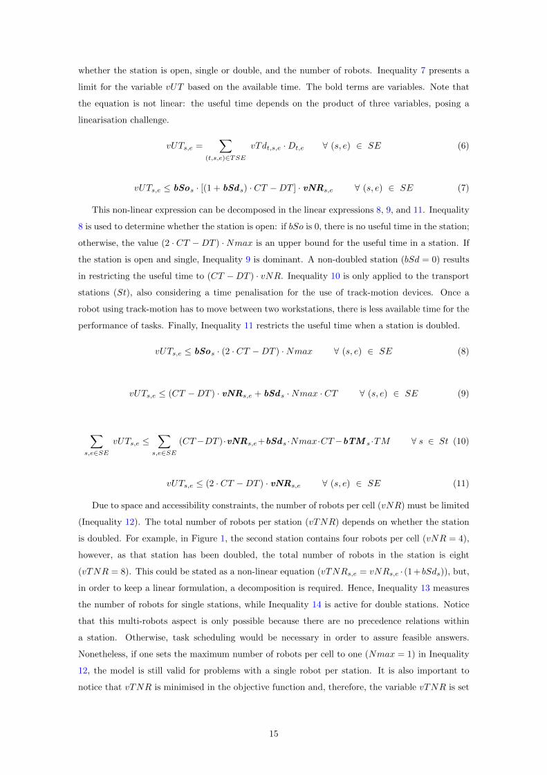
whether the station is open, single or double, and the number of robots. Inequality 7 presents a

limit for the variable vUT based on the available time. The bold terms are variables. Note that

the equation is not linear: the useful time depends on the product of three variables, posing a

linearisation challenge.

vUTs,e =∑

(t,s,e)∈TSE

vTdt,s,e ·Dt,e ∀ (s, e) ∈ SE (6)

vUTs,e ≤ bSos · [(1 + bSds) · CT −DT ] · vNRs,e ∀ (s, e) ∈ SE (7)

This non-linear expression can be decomposed in the linear expressions 8, 9, and 11. Inequality

8 is used to determine whether the station is open: if bSo is 0, there is no useful time in the station;

otherwise, the value (2 · CT −DT ) ·Nmax is an upper bound for the useful time in a station. If

the station is open and single, Inequality 9 is dominant. A non-doubled station (bSd = 0) results

in restricting the useful time to (CT −DT ) · vNR. Inequality 10 is only applied to the transport

stations (St), also considering a time penalisation for the use of track-motion devices. Once a

robot using track-motion has to move between two workstations, there is less available time for the

performance of tasks. Finally, Inequality 11 restricts the useful time when a station is doubled.

vUTs,e ≤ bSos · (2 · CT −DT ) ·Nmax ∀ (s, e) ∈ SE (8)

vUTs,e ≤ (CT −DT ) · vNRs,e + bSds ·Nmax · CT ∀ (s, e) ∈ SE (9)

∑s,e∈SE

vUTs,e ≤∑

s,e∈SE

(CT−DT )·vNRs,e+bSds ·Nmax·CT−bTM s ·TM ∀ s ∈ St (10)

vUTs,e ≤ (2 · CT −DT ) · vNRs,e ∀ (s, e) ∈ SE (11)

Due to space and accessibility constraints, the number of robots per cell (vNR) must be limited

(Inequality 12). The total number of robots per station (vTNR) depends on whether the station

is doubled. For example, in Figure 1, the second station contains four robots per cell (vNR = 4),

however, as that station has been doubled, the total number of robots in the station is eight

(vTNR = 8). This could be stated as a non-linear equation (vTNRs,e = vNRs,e · (1+ bSds)), but,

in order to keep a linear formulation, a decomposition is required. Hence, Inequality 13 measures

the number of robots for single stations, while Inequality 14 is active for double stations. Notice

that this multi-robots aspect is only possible because there are no precedence relations within

a station. Otherwise, task scheduling would be necessary in order to assure feasible answers.

Nonetheless, if one sets the maximum number of robots per cell to one (Nmax = 1) in Inequality

12, the model is still valid for problems with a single robot per station. It is also important to

notice that vTNR is minimised in the objective function and, therefore, the variable vTNR is set

15

to receive the value of the number of robots per cell (vNR) depending on the parallelism applied

to the station in Inequalities 13 and 14.∑(s,e)∈SE

vNRs,e ≤ Nmax ∀ s ∈ Sp (12)

vTNRs,e ≥ vNRs,e ∀ (s, e) ∈ SE (13)

vTNRs,e ≥ 2 · vNRs,e − 2 ·Nmax · (1− bSds) ∀ (s, e) ∈ SE (14)

The next restrictions control the shape and flow of the line. Firstly, adjacent stations can only

be opened if a previous one has already been opened (Inequality 15). A parallel station has two

identical cells (same number of robots and equipment) performing the same tasks. In order to

duplicate a cell, it firstly needs to exist and be operative. Inequality 16 assures that a station can

only be doubled if it is open. As the product flows across the line using transporter robots, it is

necessary to have at least one of them at the starting point and after all platform stations in an

alternated manner (see Figure 1). The transport cells are considered to contain only one robot

and must both start and finish the assembly line. These restrictions are represented by Equality

17 for the first station and Equality 18 for the remainder stations. Note that Equality 17 is only

applied to s = 1 and Equality 18 for s ∈ St, such that s > 1.

bSos ≤ bSos−1 ∀ s ∈ S | s > 1 (15)

bSds ≤ bSos ∀ s ∈ S (16)

∑(s,e)∈SE

vNRs,e = 1 ∀ s ∈ S | s = 1 (17)

∑s,e∈SE

vNRs,e = bSos−1 ∀ s ∈ St | s > 1 (18)

Furthermore, either when a work-piece has to be transported from a single transporter robot

into a doubled platform station or vice-versa, the transporter robot requires to be on a track-motion

device (see Figure 4), unless this transporter station has also been paralleled (Inequalities 19 and

20). In Figure 1, S2 is a platform station that has been doubled, consequently, the transporter

robot before it (S1) had to be placed on a track-motion device in order to make the robot reach both

platform cells and deposit work-pieces correctly. Alternatively, one could duplicate a transportation

cell instead, as it happened to S3, in which each transporter robot is responsible for unloading

work-pieces from different cells in the previous parallel station. Inequality 19 controls the use of

a track-motion device when moving work-pieces from single to parallel stations and Inequality 20

the other way around. Note that both restrictions are valid for s ∈ St and variables bTMs must

assume 1 when the respective transporter station is not double, i.e. bSds = 0.

bTMs ≥ (1− bSds) + bSds+1 − 1 ∀ s ∈ St | s < NS (19)

16

bTMs ≥ (1− bSds) + bSds−1 − 1 ∀ s ∈ St | s > 1 (20)

Up to this point, the model is sufficient to describe the basic Robotic Assembly Line Design

presented in Section 2. There are, however, some extra practical restrictions in the case study of

Section 4 that require more expressions. As it is stated in Section 2, some pair of tasks may require

a single station, and some tasks cannot be performed in the same station.

The modelling of extra restrictions requires an auxiliary binary variable (bTo) that controls

whether any copy of task t is performed at a station s. The link between bTo and the number of

copies of tasks allocated to a station (vTd) is given by Inequalities 21 and 22.

bTot,s ≥∑

(t,s,e)∈TSE

vTdt,s,eNt

∀ (t, s) ∈ TS (21)

bTot,s ≤∑

(t,s,e)∈TSE

vTdt,s,e ∀ (t, s) ∈ TS (22)

Due to technological restrictions (quality in precision, process control constraints), geometry

welding tasks are required to be performed on single platform stations, and all the precedent

tasks must be completed one station before the geometry tasks start. Therefore, Inequality 23 is

needed to assure that if a geometry task is performed in station s, the station cannot be doubled

(bSd = 0). The necessity of finishing all precedence tasks before a geometry task can be modelled

with a precedence relation (Inequality 3) added to the effect of an exclusion constraint due to

incompatibility (Inequality 24).

1− bTot,s ≥ bSds ∀ t ∈ SS, (t, s) ∈ TS (23)

bToti,s + bTotj ,s ≤ 1 ∀ (ti, tj) ∈ Inc, (ti, s) ∈ TS, (tj , s) ∈ TS (24)

4. Results

Two datasets were developed based on real-world data and computational tests were performed

in order to examine the influence of several model’s parameters and validate the model. This first

case study also seeks to evaluate the influences of model’s parameters in computational difficulty.

The complete mathematical formulation, including extensions (Constraints 21 and 22) and extra

restrictions (Constraints 23 and 24), was applied on them. The first dataset is composed of basic

robots and tools, whilst the second one was elaborated with the same data in an enlarged equipment

pool. These results are presented in Section 4.1.

Moreover, the model is tested on real-world data that has been collected from an automotive

industry located on the outskirts of Curtiba-PR (Brazil) and converted into practical instances in

order to analyse three case studies for different vehicle models produced in the company. Each

vehicle model requires different amount of copies of each task and the duration of each copy

may also be different depending on the vehicle model. The last model is the most complex one,

17

presenting more tasks to be performed. The production rate to meet the demand is known and the

assembly welding line ought to be designed aiming to achieve the desired cycle time at the lowest

cost. The obtained results (Table 6) for the optimal line and the line as it currently is implemented

are compared and discussed by Table 7 in Section 4.2, suggesting a potential economy of 5,9%.

To all instances, a 64 bit IntelTM i7 CPU (2.9 GHz) with 8 GB of RAM was employed using eight

threads and the IBM ILOG CPLEX Optimization Studio 12.6. Optimal solutions were found for

all instances in the first set (Section 4.1, Table 3) of the computational experiments and practical

cases (Section 4.2, Table 6) within 3600 seconds, not exceeding the solving time limit. For the

enlarged set, 18 out of 32 instances were solved within the time limit (Section 4.1, Table 4).

4.1. Parameters’ Influence Computational Study

It has been shown in Figure 5 that the dead time can be diluted between parallel stations. As the

relative importance of the dead time (DT ) in regard of the cycle time (CT ) increases, it is expected

that the line design will converge towards solutions with more parallel stations, so as to reduce

the negative effects of unproductive movements and product loading. To observe this behaviour,

computational tests were performed varying the DT from 0 to 70% of the CT . Larger values of

DT were neglected for functional reasons: no line would operate with such inefficiency and CPU

processing time is much higher when the number of maximum stations is increased. Consequences

of this fluctuation on DT can be detected on the number of robots, use of track-motions, and the

final cost.

Another computational experiment has been conducted in order to analyse the effects of chang-

ing cost structures (Askin & Zhou, 1997), i.e. setting the cost ratio between the robot cost (R) and

equipment cost (E). The chosen rations represent the practical case rate (approximately R/E = 2),

R/E = 1 (Equal: robots and equipment have comparable costs), R/E = 30 (High: robots are much

more expensive than equipment), and R/E = 1/30 (Low: robots are much cheaper than equip-

ment). Moreover, tools that are able to perform the same tasks in a reduced time are included in

the equipment pool in order to evaluate computational complexity and a possible trade-off. Faster

robots and tools combination are capable of executing the same tasks normal robots and tools do

in 60% of the time, and cost twice as much. For instance, if a welding robot that performs a copy

of task t in 10 time units and costs 10 monetary units ($) is considered, an additional welding

robot that performs the same copy of task t in 6 time units and costs 20 monetary units ($) is also

considered in the enlarged set.

Thus, the combination of both experiments (DT and R/E variations) resulted in a total of 64

instances that were summarised in Table 3 and Table 4, containing the total number of robots in

system (#vTNR), the number of opened and doubled stations (#bSo and #bSd), the number of

robots on track-motion devices (#bTM), and the computational time in seconds.

Fixed parameters were defined based on practical characteristics of robotic welding assembly

lines found in automotive industries. The desired CT is set to 1000 time units, the DT ranged

from 0 to 70% of it, the number of maximum stations (NS) is gradually increased by the user

18

depending on the DT proportion and varies from 13 to 19, the necessary time to use the track-

motion to 10% of the CT . The number of tasks is set to 40 (13 geometry tasks, 4 stud tasks and

23 finishing tasks), the number of copies of tasks varies from 1 to 20 replicas. The duration time

of each copy ranges from 21 to 77 time units, and this value is increased by 50% if the task is

performed at a transporter station. The Supporting Information is available and contains detailed

data concerning these instances.

Table 3: Results for different relative dead times (DT ) and cost ratios (R/E) with a reduced

equipment pool. #vTNR, #bSo, #bSd, and #bTM stand for total number of robots in system,

the number of opened, the number of doubled stations, and the number of robots on track-motion

devices, respectively.

DT (%) Cost ratios (R/E): Practical | Equal | High | Low

#vTNR #bSo #bSd #bTM CPU Time (s)

0 22 | 22 | 22 | 22 11 | 11 | 11 | 11 1 | 1 | 1 | 1 0 | 0 | 0 | 0 29 | 20 | 23 | 28

10 25 | 25 | 25 | 26 13 | 13 | 13 | 13 0 | 0 | 0 | 0 0 | 0 | 0 | 0 52 | 39 | 76 | 67

20 28 | 26 | 26 | 28 13 | 13 | 13 | 13 0 | 2 | 3 | 1 0 | 4 | 3 | 2 21 | 43 | 22 | 22

30 30 | 29 | 29 | 32 13 | 13 | 13 | 15 4 | 3 | 5 | 3 0 | 4 | 2 | 6 39 | 71 | 127 | 82

40 32 | 33 | 32 | 33 13 | 15 | 13 | 15 4 | 3 | 5 | 3 3 | 6 | 2 | 6 13 | 31 | 41 | 22

50 36 | 36 | 36 | 37 15 | 15 | 15 | 15 9 | 4 | 6 | 3 0 | 5 | 1 | 6 55 | 183 | 729 | 387

60 39 | 39 | 39 | 43 15 | 15 | 15 | 15 7 | 7 | 8 | 3 2 | 2 | 1 | 6 36 | 30 | 33 | 30

70 46 | 48 | 46 | 51 19 | 19 | 19 | 19 9 | 5 | 9 | 3 1 | 4 | 1 | 6 18 | 18 | 27 | 22

Table 4: Results for different relative dead times (DT ) and cost ratios (R/E) with an enlarged

equipment pool. #vTNR, #bSo, #bSd and #bTM stand for total number of robots in system,

the number of opened, the number of doubled stations and the number of robots on track-motion

devices, respectively.

DT (%) Cost ratios (R/E): Practical | Equal | High | Low

#vTNR #bSo #bSd #bTM CPU Time (s)

0 19 | 19 | 19 | 19 9 | 9 | 9 | 9 0 | 0 | 0 | 0 0 | 0 | 0 | 0 72 | 190 | 150 | 302

10 23 | 20 | 23 | 21 11 | 9 | 11 | 9 0 | 0 | 0 | 0 0 | 0 | 0 | 0 487 | 207 | 3600 | 450

20 26 | 26 | 26 | 28 11 | 13 | 13 | 13 1 | 2 | 3 | 1 0 | 4 | 3 | 2 3600 | 211 | 183 | 135

30 29 | 30 | 29 | 31 13 | 13 | 13 | 13 3 | 2 | 3 | 2 0 | 4 | 1 | 4 3600 | 2058 | 3600 | 129

40 32 | 33 | 32 | 33 13 | 15 | 13 | 15 4 | 3 | 5 | 3 3 | 6 | 2 | 6 3600 | 386 | 3600 | 220

50 36 | 35 | 36 | 35 15 | 15 | 15 | 15 9 | 3 | 7 | 3 0 | 6 | 1 | 6 3600 | 944 | 3600 | 1227

60 39 | 39 | 39 | 43 15 | 15 | 15 | 15 7 | 7 | 10 | 3 2 | 2 | 0 | 6 3600 | 3600 | 3600 | 518

70 44 | 45 | 41 | 43 17 | 17 | 15 | 15 8 | 5 | 8 | 3 2 | 4 | 1 | 6 3600 | 3600 | 3600 | 1899

Out of the 32 cases from Table 3, all of them were solved to optimality, whilst only 18 out of 32

cases from Table 4 would result in optimal solutions within the time limit. On average, the cost is

increased in 9.92% whenever there is an increase of 10% in the DT , except for the pace from 60%

to 70%. In this last case, the cost is impacted with a 16.69% raise and it clearly attests that such

relative unproductive times would result in impractical production systems.

The cost ratio experiment turned out as expected, validating the model for the practical cases:

the line layout is completely changed depending on robot and equipment relative costs. For the

cases in which the robots are much more expensive (R/E = 30), the line applies parallel stations

19

more frequently in order to take advantage on productive time enlargement. On the other hand,

the use of track-motion devices was more intensive for the opposite cases (R/E = 1/30), since the

robots are much cheaper than the tools, the model decided to allocate the equipment mainly on

platform stations, where there is no penalisation on task performing time.

Comparing Table 3 with Table 4, it is possible to state that computational times were highly

affected by allowing more equipment options in the pool. However, the increase on the DT does

not necessarily influence the solving time directly, and the instances in which the robot cost was

much lower than the equipment cost (Low R/E) expressed that this class of parameters presents

a reduced computational time to be solved. Moreover, the potential gains in saving design costs

were analysed based on the cases that reached optimality, i.e. the 18 out of 32 instances presented

in Table 4. On average, a potential economy of 1.11% was obtained and the larger difference was

found to be a 7.57% (Low R/E and 0% of DT ) cost reduction.

The optimal answer was proved for all the instances in Table 3. Still, for the enlarged equipment

pool instances (Table 4), there was a gap between the best found answer (UB) and the best possible

answer (LB) in 14 out of 32 cases. The gap for each instance is shown in Table 5. For the instances

that did not prove optimality in one hour of computational processing time, the average gap was

7.97%.

Table 5: Gaps for different relative dead times (DT ) and cost ratios (R/E) for the enlarged

equipment pool instances.

DT (%) Gap: (UB − LB)/UB

Practical R/E Equal R/E High R/E Low R/E

0 0% 0% 0% 0%

10 0% 0% 5.06% 0%

20 1.87% 0% 0% 0%

30 1.37% 0% 9.90% 0%

40 1.66% 0% 5.00% 0%

50 11.95% 0% 20.54% 0%

60 2.93% 3.26% 8.71% 0%

70 10.86% 7.32% 21.18% 0%

Lastly, the maximum number of stations (NS) for the herein reported tests were estimated

based on previous knowledge of the problem and the proposed dataset, this NS was generally

higher than necessary, i.e. a pessimistic estimation. Since all variable sets are built for all stations,

an overestimation of this parameter may include unnecessary variables to the problem.

4.2. Practical Case Study

Currently, three different vehicle models are being produced in the studied line. The validated

model explored in Section 4.1 has been employed to the data of each vehicle model in order

to conduct the practical tests. Figure A.11 shows the adapted real-world automotive industry

20

precedence diagram presented by Sikora et al. (2017b), geometry and stud tasks are indicated in

the diagram. Table A.9 presents the task times for each vehicle model as long as they are performed

in platform stations. These time durations are 50% longer if the task is performed in a transporter

station. Geometry tasks are bold-faced, stud tasks are italicised, and the remaining ones are

finishing tasks. Notice that less complex vehicles do not have all the assembly tasks that Model 3

does.

As for the other parameters, the operating line had been observed and movement time analysed

to properly determine DT and TM (respectively 50% and 10% of the CT for the practical case),

and the desired CT has also been informed by the company (1168 time units). The maximum

number of stations is empirically estimated by measuring the possible maximum length of the line

and was set to NS = 15 for the practical case study. Industrial economic parameters have been

collected, namely robot, equipment, track-motion, and platform costs. These are not always the

same for any project, they often depend on numeric studies and labour cost for installing the line.

The price parameters are average normalised values ($) taken from the last recent projects and

updates: platform cost (PCost = 4.2), track-motion cost (TMCost = 10.3), transporter robot cost

holding no equipment other than the work-piece manipulation system (RTCoste = 19.8), with a

static welding tool placed in the sideways (RTCoste = 29.9), with a static stud tool placed in the

sideways (RTCoste = 25.8), and platform robot cost holding a welding tool (RPCoste = 20.7),

or a stud tool (RPCoste = 18.4). These prices and parameters can be found in the Supporting

Information.

4.2.1. Line Design for Vehicle Models

Table 6 presents the results for the given parameters applied to each vehicle model. Naturally,

the line cost is higher for Model 3, since it is the most complex vehicle model and has more assembly

tasks than the other vehicle models.

Table 6: Results for the three vehicle models produced by the company nowadays.

Model 1 Model 2 Model 3

Cost ($) 557.5 561.5 628.6

#vTNR 24 23 26

#bSo 13 11 13

#bSd 0 2 2

#bTM 0 2 1

CPU Time (s) 40.1 31.2 32.7

The first and simplest vehicle model’s layout configuration could be designed as an exclusively

serial line in the optimal solution. Figure 7 shows the distribution of the robots and their tools’

allocation through the stations.

Analogously to the representation of the first model, Figure 8 depicts the optimal layout con-

figuration for Model 2. In this case, station paralleling has been employed in order to reduce costs

21

S8S1 S2 S3 S4 S6S5 S7 S9 S10 S11 S12 S13

Figure 7: Optimal line design for Model 1. There are 13 serial stations (S1 to S13), no double sta-

tions or track-motion were employed on the configuration. There are 24 robots in total, composed

of 17 platform robots (15 performing geometry and finishing welding tasks and 2 performing stud

tasks) and 7 transporter robots (4 performing finishing welding tasks, 1 performing stud tasks (S9)

and 2 for work-pieces handling, in the entrance and S11).

for the design project and has also shorten the line’s length. Moreover, track-motion devices are

used to reach and move work-pieces in and out of parallel stations.

S8S1 S2 S3 S4 S6S5 S7 S9 S10 S11

Figure 8: Optimal line design for Model 2. There are 11 stations (S1 to S11), 2 of them are doubled

(S3 and S6) and 2 use a track-motion device (S5 and S7). There are 23 robots in total, composed

of 16 platform robots (14 performing geometry and finishing welding tasks and 2 performing stud

tasks) and 7 transporter robots (5 performing finishing welding tasks, none performing stud tasks

and 2 for work-pieces handling, in the entrance and S7).

The optimal line design of the last and most complex vehicle model is shown in Figure 9.

In this configuration, the production layout requires 11 serial stations, 2 parallel stations and a

track-motion device. The Model 3’s line employs more features than the first one and is longer

than Model 2’s line. This fact is expected due to the larger number of tasks and copies in the

parameters.

4.2.2. Results Comparison

Figures 7, 8, and 9 represent robotic welding assembly lines for single products, as stated in the

problem’s hypotheses (Section 2). However, in the automotive industry, production systems are

22

S8S1 S2 S3 S4 S6S5 S7 S9 S10 S11 S12 S13

Figure 9: Optimal line design for Model 3. There are 13 stations (S1 to S13), 2 of them are doubled

(S7 and S8) and 1 uses a track-motion device (S9). There are 26 robots in total, composed of 18

platform robots (16 performing geometry and finishing welding tasks and 2 performing stud tasks)

and 8 transporter robots (5 performing finishing welding tasks, 2 performing stud tasks (S7) and

1 in the entrance for work-pieces handling).

frequently built to process multiple models of vehicles, giving them the property of mixed-model

assembly lines. Therefore, in order to analyse the applicability of any of these layouts, they must be

feasible for all the vehicle models, otherwise, extra robots would have to be included in the faulty

segments. Note that this approach can be seen as designing the line for the worst case. In this

situation, the layout proposed by the mathematical model for vehicle Model 3 is the only possible

candidate to assume such position and is a natural candidate to be tested for the remaining vehicle

models.

The adopted procedure was setting the variables in the optimisation model for the last vehicle

model’s design, apply it to the data of vehicle models 1 and 2 and verify its feasibility for each case.

The obtained results indicate that the configuration presented in Figure 9 was able to support the

production of the three vehicle models and, thus, allowing the cost comparison with the current

as-built line, presented in Figure 10. Alternatively, (i) some robots could be disable depending on

the vehicle model that is to be processed in order to avoiding idle times or (ii) the cycle time for

the less complex models could be even reduced in specific situations. Nonetheless, it is important

to state and remind that the costliest design for a single product is not necessarily fit to produce

all the products in a mixed-model assembly line due to the task distribution possibilities and idle

times caused by relative demands of the products. A more general approach for mixed-model lines

is a future research goal (Section 5).

Table 7 presents a comparative between the model’s solution for the optimal line design, the

configuration proposed by the engineering team, and the strictly straight line for the Model 3. The

optimal solution for Model 3 has been compared to the current as-built design and proven coherent,

reinforcing the reliability of the mathematical formulation, previously stated by the computational

results of Section 4.1. Similarly to the last procedure to test the Model 3’s layout to Models 1

and 2, the strictly serial line was simulated for the vehicle Model 3 by setting decision variables

23

Figure 10: Current as-built line. There are 13 stations (S1 to S13), 2 of them are doubled (S8 and

S9) and 1 uses a track-motion device (S7). There are 28 robots in total, composed of 20 platform

robots (19 performing geometry and finishing welding tasks and 1 performing stud tasks) and 8

transporter robots (5 performing finishing welding tasks, 2 performing stud tasks (S9) and 1 in the

entrance for work-pieces handling).

(bSd) to the desired values (always equal to zero). In other words, parallel stations had been

forbidden in the model and it was applied to the vehicle Model 3’s data. A similarity between the

optimal solution and the as-built configuration might be noticed in Table 7. However, if Figure 9

is compared to Figure 10, one can realise that the optimal design did not just reduce the number

of robots in the line, but also gave a different configuration from the current operating line as

solution.

Table 7: Comparative between the optimal line design, the configuration proposed by the engi-

neering team (as-built), and the strictly straight line for Vehicle Model 3.

Optimal As-built Serial

Cost ($) 628.6 667.7 692.4

#vTNR 26 28 30

#bSo 13 13 15

#bSd 2 2 0

#bTM 1 1 0

The costs on Table 7 are normalised due to industrial reasons and do not appear to be so large

in absolute values. The obtained relative values indicate a potential economy of approximately

5.9%, when comparing the as-built with the obtained optimal solution. Nonetheless, taking into

consideration the purchase cost of industrial welding robots and the potential of applying the model

to all robotic lines found in an automotive industry, the cost reduction on the production layout

can reach several hundred thousand dollars to be saved by the company.

Finally, this cost reduction comparison is only fair because both optimal and as-built layouts

for Model 3 (Figure 9 and Figure 10, respectively) can produce all vehicle models through the same

24

line and space, while respecting the demanded cycle time. Other layouts (Figure 7 and Figure 8)

are completely valid (and optimal) for single vehicle model processing, but are not capable of

producing all vehicle models under desired conditions of productivity rate (infeasible). Table 8

summarises which solution is optimal, feasible or infeasible for each model. Although there are

optimal solutions for Models 1 or 2 for a lower cost, notice that such solutions are not feasible

for the remaining vehicle models. Therefore, a global optimal solution could only be obtained by

Layout 3 (Figure 9).

Table 8: Feasibility verification between Models 1, 2, and 3 optimal layouts and as-built configu-

ration.

Model 1 Model 2 Model 3 Cost ($)

Layout 1 (Figure 7) Optimal Infeasible Infeasible 557.5

Layout 2 (Figure 8) Infeasible Optimal Infeasible 561.5

Layout 3 (Figure 9) Feasible Feasible Optimal 628.6

As-built (Figure 10) Feasible Feasible Feasible 667.7

5. Conclusions

Robotic welding assembly lines are frequently found in the automotive industry and defining

their production layout design is an important global and strategic decision. In this paper, the

Robotic Assembly Line Design (RALD) problem is defined and an MILP formulation is proposed

for it, taking into account several practical considerations of an RALD scenario. The proposed

model incorporates the linearisation of a cubic constraint. The developed model also allows to

explicitly evaluate costs and benefits associated to parallel stations in an exact manner.

Computational case studies were performed in Section 4.1, combining large instances of real-

world inspired cases adapted from Sikora et al. (2017b) and cost ratio principles proposed by

Askin & Zhou (1997). The existence of multiple tool alternatives and with the trade-off between

equipment cost and efficiency led to higher computational difficulties. However, 18 out of 32 of

such cases were solved to optimality within the time limit (Table 4). The main conclusions drawn

from this experiment are: (i) optimal answers tend to have more parallel stations as the dead time

increases or the robots are costly compared to the equipment, and (ii) the intense use of track-

motion devices when equipment prices are much higher than the robot ones, due to its tendency

to be more cost-effective.

Practical case studies based on the three vehicle models presented in Sikora et al. (2017b)

reached optimal answers and led to a 5.9% cost reduction in the line design for the most complex

model compared to the originally human-designed line (Section 4.2). This was only possible because

the third vehicle model line layout was able to assemble both vehicle models 1 and 2, as indicated

in Section 4.2.1. Furthermore, parallel stations evidenced its essential role when unproductive

times are considered, though paralleling was not necessarily cost-effective in every condition (e.g.

25

Figure 7).

Our study exposed how effective the formulation is when it comes to designing a robotic assem-

bly line, including practical extensions. Therefore, for future research, the proposed model can be

widened to incorporate task scheduling for each robot in the station. Moreover, the model might

be adapted to represent literature variants, such as different product models characteristics in a

mixed-model line and set-up times between them.

Acknowledgement

The authors would like to thank the financial support from Fundacao Araucaria (Agreements

141/2015, 06/2016, and 041/2017 FA-UTFPR-RENAULT), and CNPq (Grant 406507/2016-3).

References

Amen, M. (2000). Heuristic methods for cost-oriented assembly line balancing: A survey. Inter-

national Journal of Production Economics, 68 , 1–14. doi:10.1016/S0925-5273(99)00095-X.

Amen, M. (2006). Cost-oriented assembly line balancing: Model formulations, solution difficulty,

upper and lower bounds. European Journal of Operational Research, 168 , 747–770. doi:10.

1016/j.ejor.2004.07.026.

Araujo, F. F. B., Costa, A. M., & Miralles, C. (2015). Balancing parallel assembly lines with

disabled workers. European Journal of Industrial Engineering , 9 , 344–365. doi:10.1504/EJIE.

2015.069343.

Askin, R. G., & Zhou, M. (1997). A parallel station heuristic for the mixed-model production line

balancing problem. International Journal of Production Research, 35 , 3095–3106. doi:10.1080/

002075497194309.

Bard, J. F. (1989). Assembly line balancing with parallel workstations and dead time. International

Journal of Production Research, 27 , 1005–1018. doi:10.1080/00207548908942604.

Battaıa, O., & Dolgui, A. (2013). A taxonomy of line balancing problems and their solution

approaches. International Journal of Production Economics, 142 , 259–277. doi:10.1016/j.

ijpe.2012.10.020.

Baybars, l. (1986). A Survey of Exact Algorithms for the Simple Assembly Line Balancing Problem.

Management Science, 32 , 909–932. doi:10.1287/mnsc.32.8.909.

Baykasoglu, A., Tasan, S. O., Tasan, A. S., & Akyol, S. D. (2017). Modeling and solving assembly

line design problems by considering human factors with a real-life application. Human Factors

and Ergonomics In Manufacturing , 27 , 96–115. doi:10.1002/hfm.20695.

Becker, C., & Scholl, A. (2006). A survey on problems and methods in generalized assembly

line balancing. European Journal of Operational Research, 168 , 694–715. doi:10.1016/j.ejor.

2004.07.023.

26

Boysen, N., Fliedner, M., & Scholl, A. (2007). A classification of assembly line balancing problems.

European Journal of Operational Research, 183 , 674–693. doi:10.1016/j.ejor.2006.10.010.

Boysen, N., Fliedner, M., & Scholl, A. (2008). Assembly line balancing: Which model to use when?

International Journal of Production Economics, 111 , 509–528. doi:10.1016/j.ijpe.2007.02.

026.

Bukchin, J., & Rubinovitz, J. (2003). A weighted approach for assembly line design with

station paralleling and equipment selection. IIE Transactions, 35 , 73–85. doi:10.1080/

07408170390116670.

Cakir, B., Altiparmak, F., & Dengiz, B. (2011). Multi-objective optimization of a stochastic

assembly line balancing: A hybrid simulated annealing algorithm. Computers & Industrial

Engineering , 60 , 376–384. doi:10.1016/j.cie.2010.08.013.

Deckro, R. F. (1989). Balancing Cycle Time and Workstations. IIE Transactions, 21 , 106–111.

doi:10.1080/07408178908966213.

Dolgui, A., Guschinsky, N., & Levin, G. (2012). Enhanced mixed integer programming model for

a transfer line design problem. Computers & Industrial Engineering , 62 , 570–578. doi:10.1016/

j.cie.2011.11.005.

Ege, Y., Azizoglu, M., & Ozdemirel, N. E. (2009). Assembly line balancing with station paralleling.

Computers & Industrial Engineering , 57 , 1218–1225. doi:10.1016/j.cie.2009.05.014.

Essafi, M., Delorme, X., Dolgui, A., & Guschinskaya, O. (2010). A MIP approach for balancing

transfer line with complex industrial constraints. Computers & Industrial Engineering , 58 ,

393–400. doi:10.1016/j.cie.2009.04.009.

Fattahi, P., & Roshani, A. (2011). A mathematical model and ant colony algorithm for multi-

manned assembly line balancing problem. International Journal of Advanced Manufacturing

Technology , 53 , 363–378. doi:10.1007/s00170-010-2832-y.

Gao, J., Sun, L., Wang, L., & Gen, M. (2009). An efficient approach for type II robotic assembly

line balancing problems. Computers & Industrial Engineering , 56 , 1065–1080. doi:10.1016/j.

cie.2008.09.027.

Guney, Y., & Ahiska, S. S. (2014). Automation Level Optimization for an Automobile Assembly

Line. In Proceedings of the 2014 Industrial and Systems Engineering Research Conference (pp.

2209–2218).

Kim, Y. K., Kim, Y., & Kim, Y. J. (2000). Two-sided assembly line balancing: A genetic algorithm

approach. Production Planning & Control: The Management of Operations, 11 , 44–53. doi:10.

1080/095372800232478.

27

Levitin, G., Rubinovitz, J., & Shnits, B. (2006). A genetic algorithm for robotic assembly line

balancing. European Journal of Operational Research, 168 , 811–825. doi:10.1016/j.ejor.2004.

07.030.

Lopes, T. C., Sikora, C. G. S., Michels, A. S., & Magatao, L. (2017a). Mixed-model assembly lines

balancing with given buffers and product sequence: model, formulation comparisons, and case

study. Annals of Operations Research, in press, 1–26. doi:10.1007/s10479-017-2711-0.

Lopes, T. C., Sikora, C. G. S., Molina, R. G., Schibelbain, D., Rodrigues, L. C. A., & Magatao,

L. (2017b). Balancing a robotic spot welding manufacturing line: An industrial case study.

European Journal of Operational Research, 263 , 1033–1048. doi:10.1016/j.ejor.2017.06.001.

Lusa, A. (2008). A survey of the literature on the multiple or parallel assembly line balancing

problem. European J. of Industrial Engineering , 2 , 50. doi:10.1504/EJIE.2008.016329.

Michalos, G., Makris, S., Papakostas, N., Mourtzis, D., & Chryssolouris, G. (2010). Automotive

assembly technologies review: challenges and outlook for a flexible and adaptive approach. CIRP

Journal of Manufacturing Science and Technology , 2 , 81–91. doi:10.1016/j.cirpj.2009.12.

001.

Oesterle, J., Amodeo, L., & Yalaoui, F. (2017). A comparative study of Multi-Objective Al-

gorithms for the Assembly Line Balancing and Equipment Selection Problem under consid-

eration of Product Design Alternatives. Journal of Intelligent Manufacturing , (pp. 1–26).

doi:10.1007/s10845-017-1298-2.

Park, K., Park, S., & Kim, W. (1997). A heuristic for an assembly line balancing problem with

incompatibility, range, and partial precedence constraints. Computers & Industrial Engineering ,

32 , 321–332. doi:10.1016/S0360-8352(96)00301-4.

Rekiek, B., Dolgui, A., Delchambre, A., & Bratcu, A. (2002). State of art of optimization methods

for assembly line design. Annual Reviews in Control , 26 , 163–174. doi:10.1016/S1367-5788(02)

00027-5.

Rubinovitz, J., & Bukchin, J. (1991). Design and balancing of robotic assembly lines. In Proceedings

of the fourth world conference on robotics research. Pittsburgh, PA.

Rubinovitz, J., & Bukchin, J. (1993). RALB - A Heuristic Algorithm for Design and Balancing of

Robotic Assembly Lines. Annals of the CIRP , 42 , 497–500.

Sabuncuoglu, I., Erel, E., & Alp, A. (2009). Ant colony optimization for the single model U-type

assembly line balancing problem. International Journal of Production Economics, 120 , 287–300.

doi:10.1016/j.ijpe.2008.11.017.

Scholl, A. (1999). Balancing and sequencing assembly lines. (2nd ed.). Heidelberg: ed. Physica.

28

Scholl, A., & Becker, C. (2006). State-of-the-art exact and heuristic solution procedures for simple

assembly line balancing. European Journal of Operational Research, 168 , 666–693. doi:10.1016/

j.ejor.2004.07.022.

Scholl, A., Fliedner, M., & Boysen, N. (2010). ABSALOM: Balancing assembly lines with assign-

ment restrictions. European Journal of Operational Research, 200 , 688–701. doi:10.1016/j.

ejor.2009.01.049.

Sikora, C. G. S., Lopes, T. C., Lopes, H. S., & Magatao, L. (2016). Genetic algorithm for type-2

assembly line balancing. In 2015 Latin-America Congress on Computational Intelligence, LA-

CCI 2015 . doi:10.1109/LA-CCI.2015.7435951.

Sikora, C. G. S., Lopes, T. C., & Magatao, L. (2017a). Traveling worker assembly line (re)balancing

problem: model, reduction techniques, and real case studies. European Journal of Operational

Research, 259 , 949–971. doi:10.1016/j.ejor.2016.11.027.

Sikora, C. G. S., Lopes, T. C., Schibelbain, D., & Magatao, L. (2017b). Integer based formulation

for the simple assembly line balancing problem with multiple identical tasks. Computers &

Industrial Engineering , 104 , 134–144. doi:10.1016/j.cie.2016.026.

Suwannarongsri, S., & Puangdownreong, D. (2008). Optimal assembly line balancing using tabu

search with partial random permutation technique. International Journal of Management Sci-

ence and Engineering Management , 3 , 3–18. doi:10.1080/17509653.2008.10671032.

Tuncel, G., & Topaloglu, S. (2013). Assembly line balancing with positional constraints , task

assignment restrictions and station paralleling: A case in an electronics company. Computers &

Industrial Engineering , 64 , 602–609. doi:10.1016/j.cie.2012.11.006.

Yazgan, H. R., Beypinar, I., Boran, S., & Ocak, C. (2011). A new algorithm and multi-response

Taguchi method to solve line balancing problem in an automotive industry. International Journal

of Advanced Manufacturing Technology , 57 , 379–392. doi:10.1007/s00170-011-3291-9.

Yoosefelahi, A., Aminnayeri, M., Mosadegh, H., & Ardakani, H. D. (2012). Type II robotic

assembly line balancing problem: An evolution strategies algorithm for a multi-objective model.

Journal of Manufacturing Systems, 31 , 139–151. doi:10.1016/j.jmsy.2011.10.002.

Appendix A. Practical Study Case Data

The following precedence diagram (Figure A.11) and list of tasks and their number of copies

and duration for each model (Table A.9) were used for the practical case studies in Section 4.2.

29

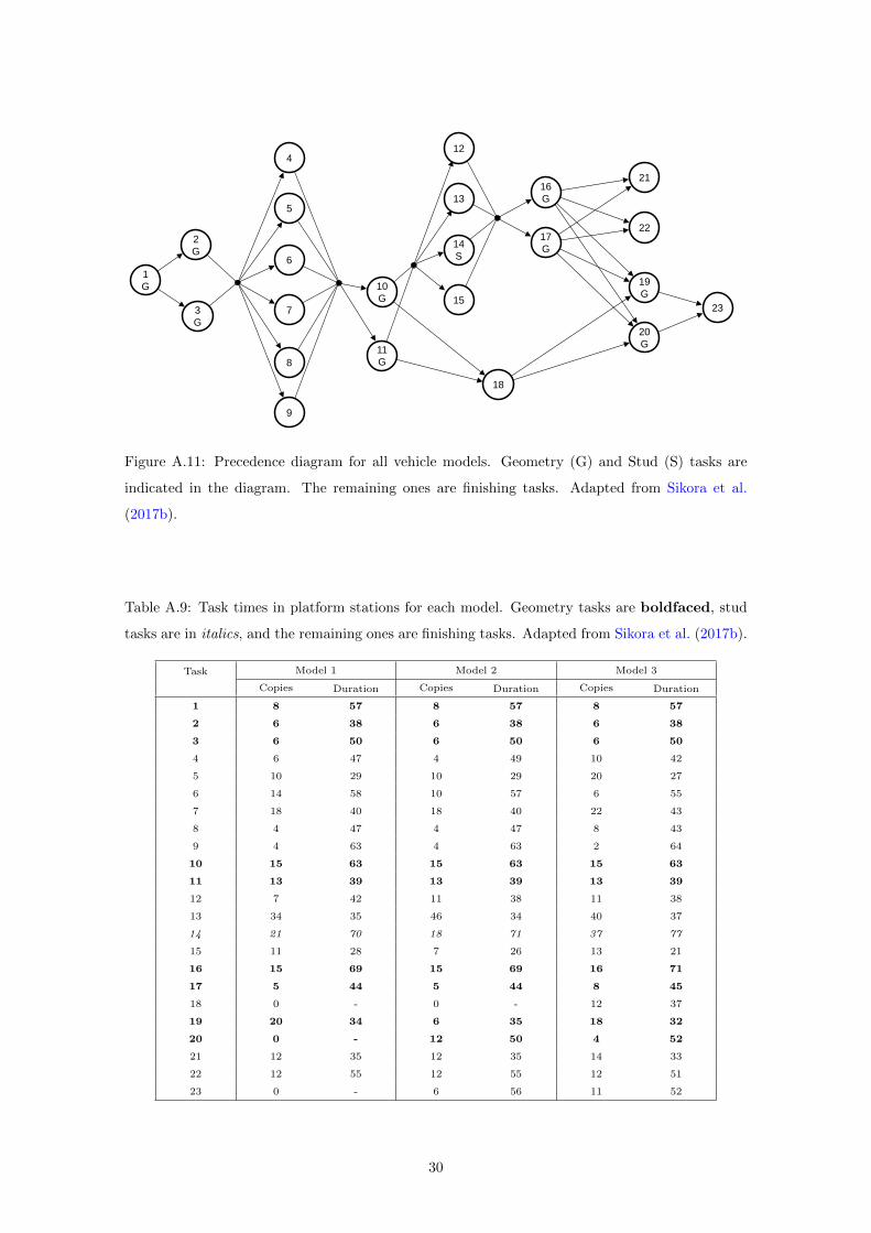
21

22

23

1

G

3

G

2

G

4

5

6

7

8

9

10

G

11

G

12

13

14

S

15

16

G

19

G

18

17

G

20

G

Figure A.11: Precedence diagram for all vehicle models. Geometry (G) and Stud (S) tasks are

indicated in the diagram. The remaining ones are finishing tasks. Adapted from Sikora et al.

(2017b).

Table A.9: Task times in platform stations for each model. Geometry tasks are boldfaced, stud

tasks are in italics, and the remaining ones are finishing tasks. Adapted from Sikora et al. (2017b).

Task Model 1 Model 2 Model 3

Copies Duration Copies Duration Copies Duration

1 8 57 8 57 8 57

2 6 38 6 38 6 38

3 6 50 6 50 6 50

4 6 47 4 49 10 42

5 10 29 10 29 20 27

6 14 58 10 57 6 55

7 18 40 18 40 22 43

8 4 47 4 47 8 43

9 4 63 4 63 2 64

10 15 63 15 63 15 63

11 13 39 13 39 13 39

12 7 42 11 38 11 38

13 34 35 46 34 40 37

14 21 70 18 71 37 77

15 11 28 7 26 13 21

16 15 69 15 69 16 71

17 5 44 5 44 8 45

18 0 - 0 - 12 37

19 20 34 6 35 18 32

20 0 - 12 50 4 52

21 12 35 12 35 14 33

22 12 55 12 55 12 51

23 0 - 6 56 11 52

30