Minimizing production costs for a robotic assembly systemmaged/publications/Minimizing Production Costs.pdf · Minimizing production costs for a robotic assembly system ... School

Engineering Costs and Production Economics, 2 1 ( 199 I ) 8 1-92 81 Elsevier

Minimizing production costs for a robotic assembly system

Maged M. Dessouky

Department oflndustrial Engineeringand Operations Research, Universltv of California, Berkeley, CA 94720, USA

and James R. Wilson

School qflndustrial Engineering, Purdue University, West Lafayette. IN 47907, USA

(Accepted June 22, 1990)

Abstract

The objective of this study is to minimize the expected present worth of the production costs incurred over the operational life of a robotic assembly system that is integrated with an Automatic Storage/Retrieval System (AS/RS). Produc- tion costs include inventory cost and capital cost of equipment. Inventory cost consists of ordering, holding, and lost- production costs; and all of these costs depend on the scheduling policy for the assembly robots as well as the inventory policy for the AS/RS. Capital cost of equipment depends on the number of depalletizer robots and the number of assembly robots. To identify the minimum-cost design for a certain automotive assembly operation from a given set of alternative system configurations, we present a simulation experiment in which independent replications of each alternative are controlled by a statistical ranking-and-selection procedure that has been adapted to simulation.

1. Introduction

In the past several years, many companies have invested large amounts of capital to implement Automatic Storage/Retrieval Systems ( AS/RSs). An AS/RS is defined as “a combination of equipment and controls which handles, stores, and retrieves materials with precision, accuracy, and speed under a defined degree of automa- tion” [ 11. Such systems range from simple man- ually controlled order-picking machines operating in small storage structures to complex computer-controlled storage/retrieval systems that are totally integrated into the manufacturing and distribution process [ 2 1. The main purpose of an AS/RS is to centralize the storage and retrieval operations and thus to increase the efli- ciency of these operations. In this study we con- centrate on AS/RSs that are integrated into the manufacturing process.

Integration of storage, retrieval, and production operations requires a direct linkage between the inventory control policy of the AS/RS and the scheduling policy of the manufacturing sys-

tern. This linkage accentuates the need for an effective inventory control policy that prevents stockouts at the AS/RS and thus ensures uninter- rupted production while simultaneously main- taining an acceptably low level of inventory. In this paper we present a simulation-based method for identifying minimum cost inventory-control and production-scheduling policies in such an integrated manufacturing system. A key feature of this approach is the use of a statistical ranking- and-selection procedure that has been adapted to simulation experiments. Thus in the comparison of alternative operating policies, we can determine the appropriate number of independent replications for each individual policy by taking into account (a) a user-specified threshold on practically significant differences in the average response between policies, and (b) possible disparities among the response variances for different policies. Note that statistical techniques based on classical analysis of variance (ANOVA ) cannot easily handle these items.

This paper is organized as follows. Section 2 contains a description of a particular automotive

0 167-l 88X/9 l/$03.50 0 199 I-Elsevier Science Publishers B.V.

82

assembly operation to which our methodology is applied. In Section 3 we formulate the general cost function for such an assembly system. Sec- tion 4 details the design of a large-scale simulation experiment for this system, including (a) the operating policies to be compared, (b) the simulation model used to implement those policies, and (c) the statistical procedure used to control the execution of each policy and to compare the resulting outputs. The analysis of the experimental results is presented in Section 5. We summa- rize our conclusions in Section 6. Although this paper is based on Dessouky [ 3 1, some of our results were originally presented in Caruso and Dessouky [ 4 1.

2. System description

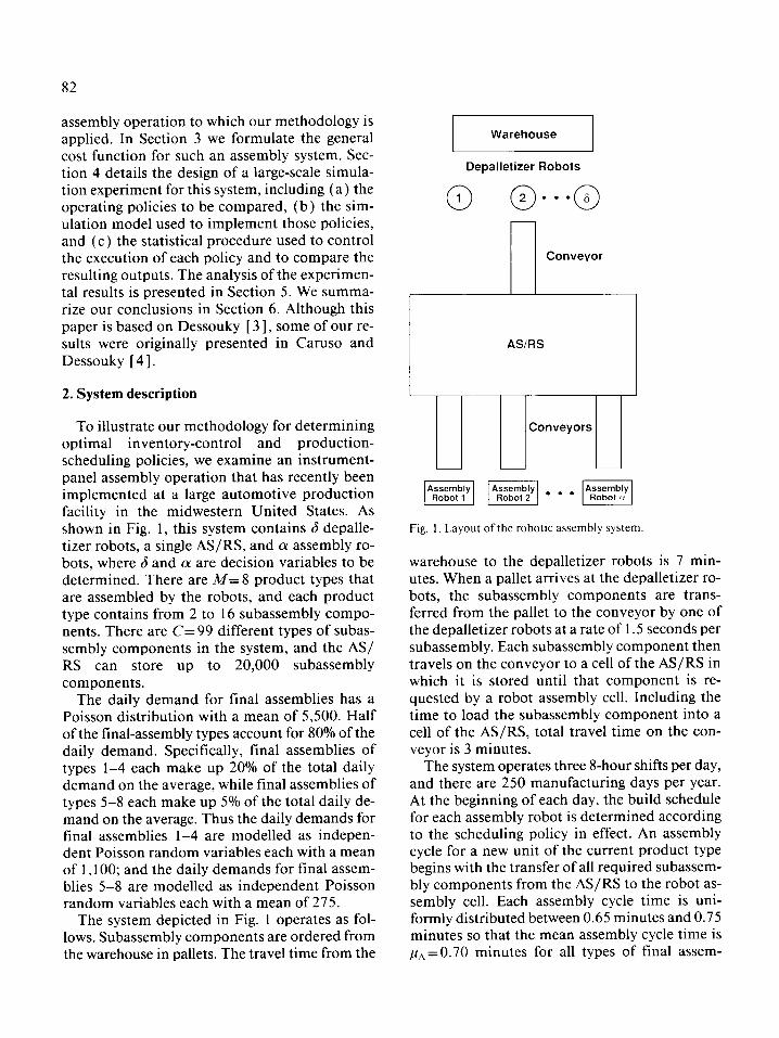
To illustrate our methodology for determining optimal inventory-control and production- scheduling policies, we examine an instrument- panel assembly operation that has recently been implemented at a large automotive production facility in the midwestern United States. As shown in Fig. 1, this system contains 6 depalletizer robots, a single AS/R& and cx assembly robots, where 6 and (Y are decision variables to be determined. There are M= 8 product types that are assembled by the robots, and each product type contains from 2 to 16 subassembly components. There are C=99 different types of subassembly components in the system, and the AS/ RS can store up to 20,000 subassembly components.

The daily demand for final assemblies has a Poisson distribution with a mean of 5,500. Half of the final-assembly types account for 80% of the daily demand. Specifically, final assemblies of types l-4 each make up 20% of the total daily demand on the average, while final assemblies of types 5-8 each make up 5% of the total daily demand on the average. Thus the daily demands for final assemblies l-4 are modelled as independent Poisson random variables each with a mean of 1,100; and the daily demands for final assemblies 5-8 are modelled as independent Poisson random variables each with a mean of 275.

The system depicted in Fig. 1 operates as follows. Subassembly components are ordered from the warehouse in pallets. The travel time from the

r---Ezq Depalletizer Robots

@ (Q-•*@

n Conveyor

AS/US

1

Conveyors

Fig. I Layout of the robotic assembly system.

warehouse to the depalletizer robots is 7 minutes. When a pallet arrives at the depalletizer robots, the subassembly components are trans- ferred from the pallet to the conveyor by one of the depalletizer robots at a rate of 1.5 seconds per subassembly. Each subassembly component then travels on the conveyor to a cell of the AS/RS in which it is stored until that component is re- quested by a robot assembly cell. Including the time to load the subassembly component into a cell of the AS/R& total travel time on the conveyor is 3 minutes.

The system operates three &hour shifts per day, and there are 250 manufacturing days per year. At the beginning of each day, the build schedule for each assembly robot is determined according to the scheduling policy in effect. An assembly cycle for a new unit of the current product type begins with the transfer of all required subassembly components from the AS/RS to the robot assembly cell. Each assembly cycle time is uni- formly distributed between 0.65 minutes and 0.75 minutes so that the mean assembly cycle time is fi,=O.70 minutes for all types of final assem-

blies. A lo-minute delay is required to change over an assembly robot to production of a different type of final assembly. If an assembly robot finishes its daily build schedule early, then that robot remains idle for the rest of the day. The other possibility is that an assembly robot may fail to complete its build schedule before the end of the day.

Since the daily demand for final assemblies is random, there is a nonzero probability that a day’s demand cannot be satisfied. This probability is a complicated function of the following factors: (a) the system’s maximum production capacity (that is, the maximum throughput rate of the assembly and depalletizer robots); (b) the number of changeovers and the associated delays that are required each day for each of the assembly robots; and (c) the inventory levels in the AS/ RS for the required subassembly components. A lower bound for the probability of unsatisfied demand occurring on any given day is the probability that the daily demand exceeds the maximum daily production rate 144Ocu/~~ for the assembly robot(s). If backlogged demands were allowed in this situation, then excessive slippage in the production schedule could occur on days that most or all of the production capacity must be devoted to eliminating the accumulated back- log. To avoid such slippage, we do not allow backlogging; instead a lost-production cost is charged for each unit of unsatisfied demand that occurs during the day.

An inventory review for the AS/RS occurs after every delivery of a subassembly component to a robot assembly cell. When the inventory level of a subassembly component in the AS/RS falls below the reorder point, a replenishment order is sent to the warehouse. The average lead time to fill a replenishment order is A=45 minutes; and this includes pallet-loading time at the warehouse, travel time to the AS/RS, and waiting time at the depalletizer robots. The inventory left in the AS/RS at the end of the day is carried over to the next day.

The specific cost components in this system are given below. ( 1) The holding cost is $0.35 per component per

day for each type of subassembly. (2 ) The ordering cost is $5.00 per order for each

type of subassembly.

(3)

(4)

(5)

(6)

83

The lost-production cost is $5.00 per unit for each type of final assembly. The capital cost of a depalletizer robot is $750,000. The capital cost of an assembly robot is $750,000. The rate of return for the organization is 15% per year.

3. General problem formulation

The cost structure described in this section is a generalization of the costs associated with the specific robotic assembly system described in Section 2. In general the assembly system under consideration produces a set of M final products {A,:j= 1 ,...,M} with respective daily demands {D,:j= 1 ,...,w. The subassembly requirements of the jth assembly are summarized in the vector B,- [B ,,,..., B,,], where B,, is the number of units of subassembly c required to produce one unit of assembly j (j= l,..., M, c= l,..., C). The controllable factors in the production process are enum- erated below.

( 1) The order of manufacturing final products by the kth assembly robot is summarized in the vector Qk= [L&,,...,QkM], where the assignment 52,, =j means that product type j is the uth product type to be manufactured by robot k in satis- fying the daily demand (k= l,..., a; U, j= l,..., M). Thus the o XM matrix

QG ,“’ [ 1 a

represents the overall build schedule for a day as determined by the production-scheduling policy in effect.

(2) The inventory policy for stocking subassembly c (c= 1 ,...,C) is represented by the reorder point R, and the order quantity Qc. The overall inventory policy is summarized by the associated vectors R= [R,,...,R,] and Q= [Q,,...,Qcl.

(3 ) The number of depalletizer assembly robots is symbolized by 6.

(4) The number of assembly robots is symbolized by cy.

84

The problem is to determine s), R, Q, 6, and cy to minimize the expected present worth of the total production cost incurred over the operational life of the system.

The total production cost associated with such a robotic assembly system includes inventory cost and capital cost of equipment. The inventory cost depends on the time-averaged inventory level, the number of replenishment orders placed, and the loss of production due to part unavailability or changeover delays. The capital cost of equipment is determined by the number of depalletizer robots and the number of assembly robots. The present worth of the total production cost can be expressed formally as:

r 1 7‘

PW= 1 (l+i)-’ i: (HJ,.,+KJ,.,)+ f P,L,f /=I <‘= I ,= I

where PW=

T =

i =

Hc =

Z <I =

Kc =

J,, =

P, =

L,, =

Y = z =

+GY+o!z (1)

Present worth of total production cost incurred over the planning horizon, Number of time periods (years) in the planning horizon, The organization’s rate of return per time period, Holding cost per item per time period for subassembly c, Time-averaged inventory level over time period t for subassembly c, Ordering cost per replenishment order for subassembly c, Number of replenishment orders for subassembly c placed during time period t, Lost-production cost per item for final assembly j, Total lost production for linal assembly j during time period t, Capital cost of a depalletizer robot, and Capital cost of an assembly robot.

Several remarks should be made about the formulation ( 1) of the present worth of the production costs. The subexpression 6Y+ aZ represents the expected present worth of the investment in robots, and this includes operating and mainte- nance costs as well as the salvage value of the robots. Note that PW must be treated as a random

variable because production requirements per time period, lead times for replenishment orders, and successive assembly cycle times exhibit sub- stantial random variation. Thus the main objective of this study is to minimize E [ PW (SL, R, Q, 6, a) ] over a prespecified set of values for the decision variables 6 and (Y and over selected policies for setting the matrices 52, R, and Q. During the time period t we accumulate the random vectors I,- [I 11,...,~c11, Jr- [JwrJc,l, and L, E [ L,,,...,L,,,] respectively representing the inventory levels, ordering levels, and lost-production levels for that period. We assume that the system is in steady-state operation so that the stochastic process { [Z,,J,,L,] : t= l,...,T} is covar- iance stationary and the expected periodic cost EPC of operating the system for one time period (exclusive of the cost of robots) is given by

EPC= C (H,.E[Z,.,] +K,.E[J,.,]) (‘= I

.14

+ Ca,E[L,,l, t= l,...,T (2) /=I

Taking expectations in ( 1) and substituting (2 ) into the resulting expression, we obtain a com- putational formula for the objective function to be minimized

E[PW]=[(;;;);.‘]EPC+dY+aZ (3)

Thus EPC is the only component of the objective function (3) that must be estimated by simulation, and this observation substantially reduces the amount of simulated experimentation that must be performed to identify the optimal inventory-control and production-scheduling policies.

4. Design of the simulation experiment

In this section we describe the alternative operating policies (scenarios) to be compared, the simulation model used to implement those policies, and the statistical procedure used to compare those policies.

85

4.1 Alternative scenarios

Within the scope of the application detailed in Section 2, we identified three relevant settings for each of the four controllable factors. Thus, we specified 81 alternative operating policies or scenarios to be compared in determining the minimum cost design for the robotic assembly system.

The number of assembly robots ranges from 3 to 5. At least 3 assembly robots are required to satisfy the expected daily demand. On the other hand, there is only enough physical space to ac- commodate 5 assembly robots.

The number of depalletizer robots ranges from 1 to 3. Of course at least 1 depalletizer robot is required, and the system has enough physical space for up to 3 depalletizer robots.

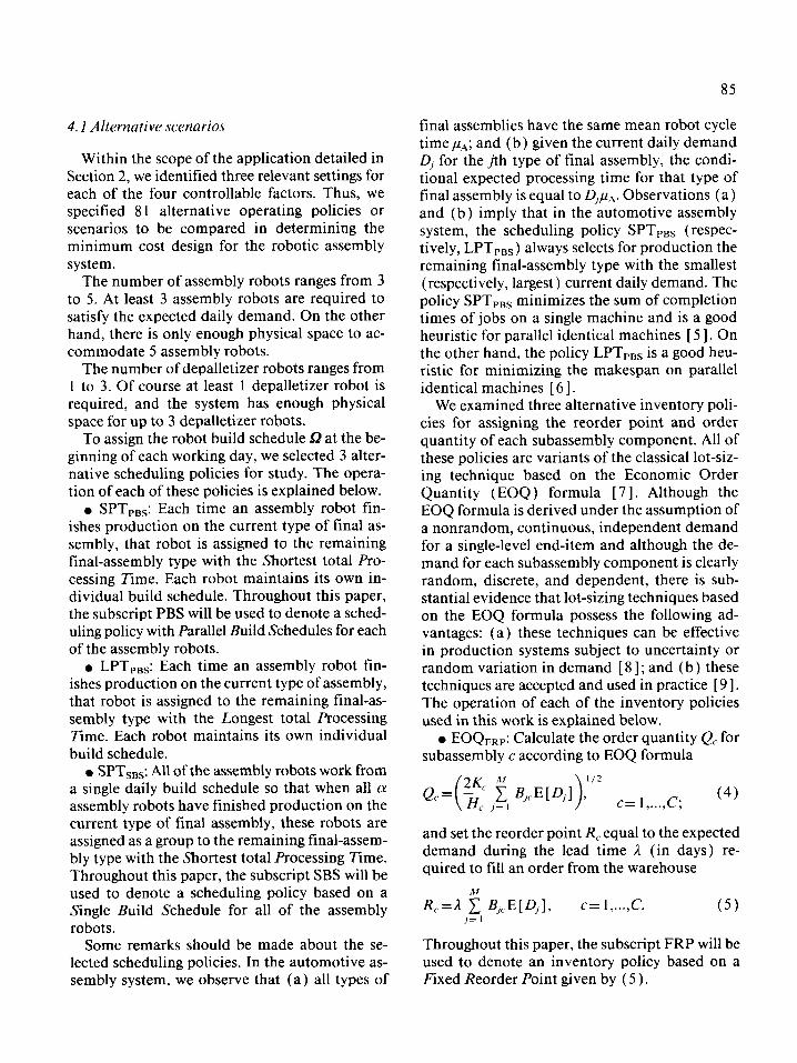
To assign the robot build schedule g at the beginning of each working day, we selected 3 alternative scheduling policies for study. The operation of each of these policies is explained below. l SPT& Each time an assembly robot fin-

ishes production on the current type of final assembly, that robot is assigned to the remaining final-assembly type with the Shortest total Pro- cessing Zme. Each robot maintains its own individual build schedule. Throughout this paper, the subscript PBS will be used to denote a scheduling policy with Parallel Build Schedules for each of the assembly robots. l LPTp& Each time an assembly robot lin-

ishes production on the current type of assembly, that robot is assigned to the remaining final-assembly type with the Longest total Processing 7ime. Each robot maintains its own individual build schedule. l SPTsss: All of the assembly robots work from

a single daily build schedule so that when all cy assembly robots have finished production on the current type of final assembly, these robots are assigned as a group to the remaining linal-assembly type with the Shortest total Processing fime. Throughout this paper, the subscript SBS will be used to denote a scheduling policy based on a Single Build Schedule for all of the assembly robots.

Some remarks should be made about the selected scheduling policies. In the automotive assembly system, we observe that (a) all types of

final assemblies have the same mean robot cycle time p+,; and (b) given the current daily demand D, for the fib type of final assembly, the condi- tional expected processing time for that type of final assembly is equal to D,,uuA. Observations (a) and (b) imply that in the automotive assembly system, the scheduling policy SPTpss (respectively, LPTpBs) always selects for production the remaining final-assembly type with the smallest (respectively, largest ) current daily demand. The policy SPTpes minimizes the sum of completion times of jobs on a single machine and is a good heuristic for parallel identical machines [ 5 J. On the other hand, the policy LPTpes is a good heuristic for minimizing the makespan on parallel identical machines [ 6 1.

We examined three alternative inventory policies for assigning the reorder point and order quantity of each subassembly component. All of these policies are variants of the classical lot-sizing technique based on the Economic Order Quantity (EOQ) formula [ 71. Although the EOQ formula is derived under the assumption of a nonrandom, continuous, independent demand for a single-level end-item and although the demand for each subassembly component is clearly random, discrete, and dependent, there is sub- stantial evidence that lot-sizing techniques based on the EOQ formula possess the following advantages: (a) these techniques can be effective in production systems subject to uncertainty or random variation in demand [ 8 1; and (b) these techniques are accepted and used in practice [ 9 1. The operation of each of the inventory policies used in this work is explained below. l EOQFRP: Calculate the order quantity Qc for

subassembly c according to EOQ formula

Qc=(% ; &E[D,l),“* c=l C. (4) ‘ J--1 >“‘, ,

and set the reorder point R, equal to the expected demand during the lead time J. (in days) required to fill an order from the warehouse

R,=/I g B,,E[D,], c= l,...,C. (5) ,=I

Throughout this paper, the subscript FRP will be used to denote an inventory policy based on a Fixed Reorder Point given by ( 5 ).

86

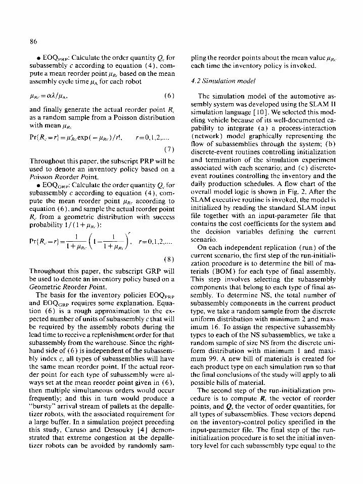
l EOQ,w: Calculate the order quantity Qc for subassembly c according to equation ( 4 ) , compute a mean reorder point pLRc based on the mean assembly cycle time p+, for each robot

and finally generate the actual reorder point R, as a random sample from a Poisson distribution with mean ,uRc

Pr{R,.=r}=p&exp( --p&)/r!, r=0,1,2 )....

(7)

Throughout this paper, the subscript PRP will be used to denote an inventory policy based on a Poisson Reorder Point. l EOQGRP: Calculate the order quantity Q, for

subassembly c according to equation (4)) compute the mean reorder point PRc according to equation ( 6 ) , and sample the actual reorder point R, from a geometric distribution with success probability 1 / ( 1 + ,u~~):

Pr{ R,. = r} = I+:-,,:( l-&J, r=0,1,2 ,....

(8)

Throughout this paper, the subscript GRP will be used to denote an inventory policy based on a Geometric Reorder Point.

The basis for the inventory policies EOQpRp

and EOQGRp requires some explanation. Equa- tion (6) is a rough approximation to the expected number of units of subassembly c that will be required by the assembly robots during the lead time to receive a replenishment order for that subassembly from the warehouse. Since the right- hand side of (6) is independent of the subassembly index c, all types of subassemblies will have the same mean reorder point. If the actual reorder point for each type of subassembly were always set at the mean reorder point given in (6 ), then multiple simultaneous orders would occur frequently; and this in turn would produce a “bursty” arrival stream of pallets at the depalletizer robots, with the associated requirement for a large buffer. In a simulation project preceding this study, Caruso and Dessouky [4] demon- strated that extreme congestion at the depalletizer robots can be avoided by randomly sam-

pling the reorder points about the mean value & each time the inventory policy is invoked.

4.2 Simulation model

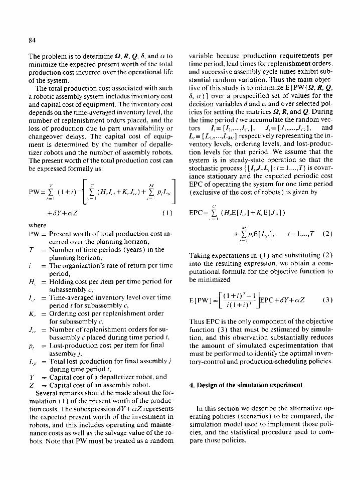
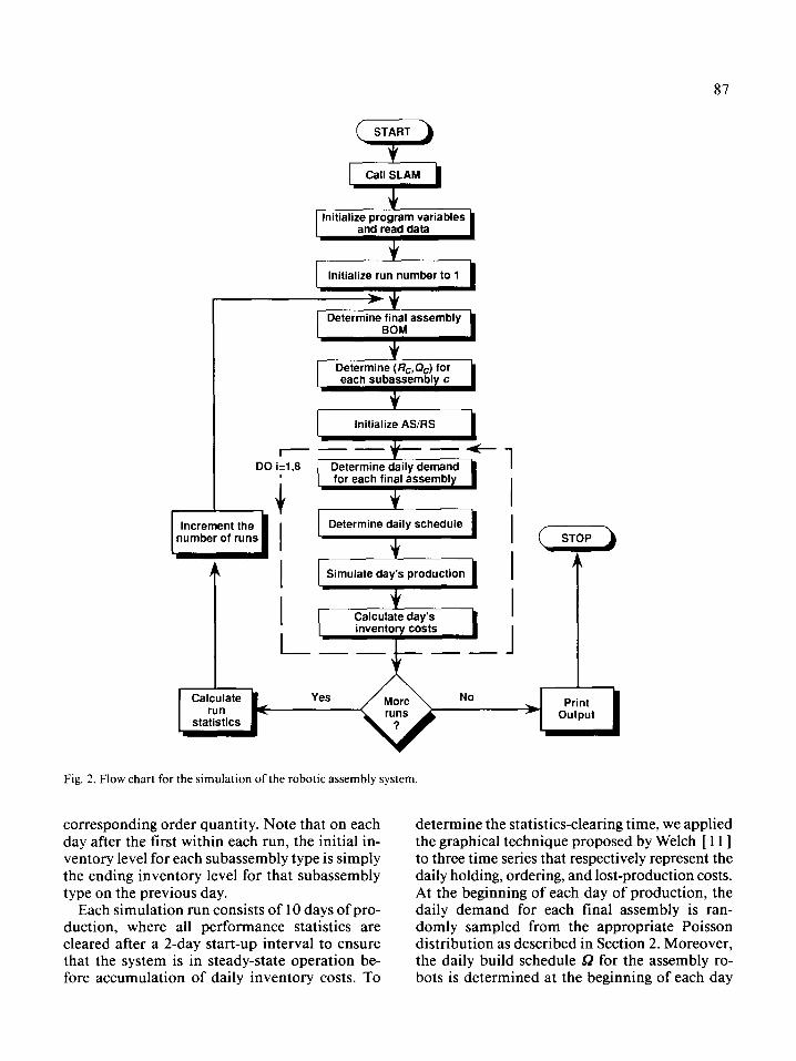
The simulation model of the automotive assembly system was developed using the SLAM II simulation language [ lo]. We selected this modeling vehicle because of its well-documented ca- pability to integrate (a) a process-interaction (network) model graphically representing the flow of subassemblies through the system; (b) discrete-event routines controlling initialization and termination of the simulation experiment associated with each scenario; and (c) discrete- event routines controlling the inventory and the daily production schedules. A flow chart of the overall model logic is shown in Fig. 2. After the SLAM executive routine is invoked, the model is initialized by reading the standard SLAM input file together with an input-parameter file that contains the cost coefficients for the system and the decision variables defining the current scenario.

On each independent replication (run) of the current scenario, the first step of the run-initialization procedure is to determine the bill of materials (BOM) for each type of final assembly. This step involves selecting the subassembly components that belong to each type of final assembly. To determine NS, the total number of subassembly components in the current product type, we take a random sample from the discrete uniform distribution with minimum 2 and maximum 16. To assign the respective subassembly types to each of the NS subassemblies, we take a random sample of size NS from the discrete uniform distribution with minimum 1 and maximum 99. A new bill of materials is created for each product type on each simulation run so that the final conclusions of the study will apply to all possible bills of material.

The second step of the run-initialization procedure is to compute R, the vector of reorder points, and Q, the vector of order quantities, for all types of subassemblies. These vectors depend on the inventory-control policy specified in the input-parameter tile. The final step of the run- initialization procedure is to set the initial inventory level for each subassembly type equal to the

87

Initialize run number to 1

*T Determine final assembly

Determine (Rc,Oc) for each subassembly c

JI

Initialize ASKS c

DO i=l 8 r*ii+

Increment the number of runs

1 I

STOP IL, I

J

I No

Fig. 2. Flow chart for the simulation of the robotic assembly system.

corresponding order quantity. Note that on each day after the first within each run, the initial inventory level for each subassembly type is simply the ending inventory level for that subassembly type on the previous day.

Each simulation run consists of 10 days of production, where all performance statistics are cleared after a 2-day start-up interval to ensure that the system is in steady-state operation before accumulation of daily inventory costs. To

determine the statistics-clearing time, we applied the graphical technique proposed by Welch [ 111 to three time series that respectively represent the daily holding, ordering, and lost-production costs. At the beginning of each day of production, the daily demand for each final assembly is randomly sampled from the appropriate Poisson distribution as described in Section 2. Moreover, the daily build schedule Q for the assembly robots is determined at the beginning of each day

88

using the production-scheduling policy specified in the input-parameter tile. The overall statistics on daily inventory costs are updated at the end of each day of simulated operation.

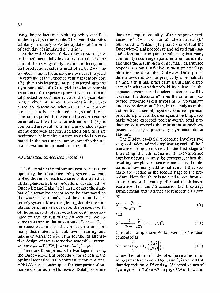
At the end of each IO-day simulation run, the estimated mean daily inventory cost (that is, the sum of the average daily holding, ordering, and lost-production costs) is multiplied by 250 (the number of manufacturing days per year) to yield an estimate of the expected yearly inventory cost (2); then this latter quantity is inserted into the right-hand side of (3) to yield the latest sample estimate of the expected present worth of the total production cost incurred over the 5-year planning horizon. A run-control event is then exe- cuted to determine whether (a) the current scenario can be terminated, or (b) additional runs are required. If the current scenario can be terminated, then the final estimator of (3) is computed across all runs in the associated experiment; otherwise the required additional runs are performed before the current scenario is terminated. In the next subsection we describe the statistical-estimation procedure in detail.

4.3 Statistical comparison procedure

To determine the minimum-cost scenario for operating the robotic assembly system, we controlled the runs of each scenario with a statistical ranking-and-selection procedure developed by Dudewicz and Dalal [ 12 1. Let k denote the number of alternative scenarios to be compared so that k= 8 1 in our analysis of the automotive assembly system. Moreover, let X,, denote the simulation response (in our case, the present worth of the simulated total production cost) accumulated on the uth run of the /th scenario. We assume that the simulation outputs (X,,: U= 1,2,...} on successive runs of the Ith scenario are normally distributed with unknown mean puxl and unknown variance I&. Thus for the Ith alternative design of the automotive assembly system, we havepx,=E[PW,], where I= 1,2 ,..., k.

There are three principal advantages in using the Dudewicz-Dalal procedure for selecting the optimal scenario: (a) in contrast to conventional ANOVA-based techniques for comparing alternative scenarios, the Dudewicz-Dalal procedure

does not require equality of the response variances {&:I= l,...,k} for all alternatives; (b) Sullivan and Wilson [ 131 have shown that the Dudewicz-Dalal procedure and related ranking- and-selection techniques are robust against many commonly occurring departures from normality; and thus the assumption of normally distributed responses is not restrictive in most practical ap- plications; and (c) the Dudewicz-Dalal procedure allows the user to prespecify a probability P* and a minimal practically significant differ- ence d* such that with probability at least P*, the expected response of the selected scenario will lie less than the distance d* from the minimum expected response taken across all k alternatives under consideration. Thus, in the analysis of the automotive assembly system, this comparison procedure protects the user against picking a scenario whose expected present-worth total production cost exceeds the minimum of such expected costs by a practically significant dollar amount.

The Dudewicz-Dalal procedure involves two stages of independently replicating each of the k scenarios to be compared. In the first stage of simulating the Ith scenario, a user-specified number of runs n, must be performed; then the resulting sample variance estimate is used to determine how many additional runs of that scenario are needed in the second stage of the procedure. Note that there is no need to synchronize or coordinate the runs performed on different scenarios. For the fth scenario, the first-stage sample mean and variance are respectively given

by

(9)

and

(10)

The total sample size N/ for scenario 1 is then computed as

N,=max{n,+ 1, [%I}, (11)

where the notation [zl denotes the smallest inte- ger greater than or equal to z, and h 1 is a constant that depends on k, P* and no. (Selected values of h, are given in Table 9.7 on page 329 of Law and

89

Kelton [ 14 1, and a FORTRAN 77 program for computing h, is available from the authors on request. )

In the second stage of simulating the Ith scenario, we perform N,-n, additional runs to obtain the second-stage sample mean

(12)

Weighting factors for the sample means of the two stages are respectively defined by

no w’=N, l+ i cc N/

h:S:/(Py - l)($- 1)y2}

and

w;=1-IV, (13)

so that the final weighted-average estimator of pLxI is

X, = IV/X, + w;X; (14)

for I=1 ,.,.,k. We select the scenario yielding min{Z,: 1= l,... ,kj, the smallest weighted-average response.

In the analysis of the automotive assembly system, we tookP*=0.95 and d*=$750,000. These parameter values ensure that with probability at least equal to 95%, the expected present worth of the total production cost for the selected scenario will differ from the corresponding cost of the optimal scenario by less than the cost of a single robot. In view of the recommendation of Law and Kelton [ 141 that no should be greater than or equal to 15, we took no=25 in the experiments discussed in the next section.

5. Analysis of experimental results

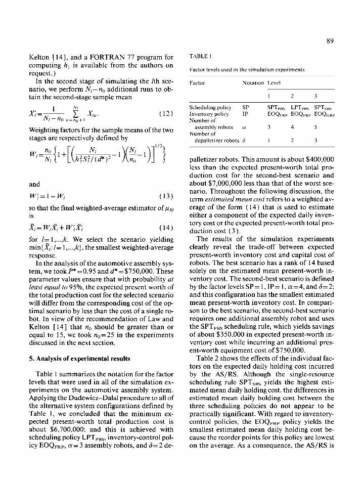
Table 1 summarizes the notation for the factor levels that were used in all of the simulation experiments on the automotive assembly system. Applying the Dudewicz-Dalal procedure to all of the alternative system configurations defined by Table 1, we concluded that the minimum expected present-worth total production cost is about $6,700,000; and this is achieved with scheduling policy LPTPBS, inventory-control policy EOQFRP, a = 3 assembly robots, and 6= 2 de-

TABLE I

Factor levels used in the simulation experiments

Factor Notation Level

I 2 3

Scheduling policy SP SPTpes LPTpss SPTsss Inventory policy IP EQQFRP EOQPRP E0Qw-w Number of

assembly robots LY 3 4 5

Number of

depalletizer robots 6 I 2 3

palletizer robots. This amount is about $400,000 less than the expected present-worth total production cost for the second-best scenario and about $7,000,000 less than that of the worst scenario. Throughout the following discussion, the term estimated mean cost refers to a weighted average of the form ( 14) that is used to estimate either a component of the expected daily inventory cost or the expected present-worth total production cost ( 3 ).

The results of the simulation experiments clearly reveal the trade-off between expected present-worth inventory cost and capital cost of robots. The best scenario has a rank of 14 based solely on the estimated mean present-worth inventory cost. The second-best scenario is defined by the factor levels SP = 1, IP = 1, a = 4, and 6= 2; and this configuration has the smallest estimated mean present-worth inventory cost. In comparison to the best scenario, the second-best scenario requires one additional assembly robot and uses the SPTpes scheduling rule, which yields savings of about $350,000 in expected present-worth inventory cost while incurring an additional present-worth equipment cost of $750,000.

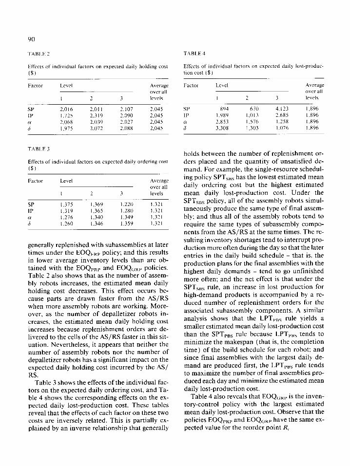
Table 2 shows the effects of the individual factors on the expected daily holding cost incurred by the AS/RS. Although the single-resource scheduling rule SPTsss yields the highest estimated mean daily holding cost, the differences in estimated mean daily holding cost between the three scheduling policies do not appear to be practically significant. With regard to inventory- control policies, the EOQpRp policy yields the smallest estimated mean daily holding cost because the reorder points for this policy are lowest on the average. As a consequence, the AS/RS is

90

TABLE 2 TABLE 4

Effects of indlwdual factors on expected daily holding cost

($)

Factor Level

1 2 3

Average

over all

levels

Effects of individual factors on expected daily lost-produc-

tlon cost ($)

Factor Level

I 2 3

Average

over all

levels

SP 2,016 2.01 I 2.107 2,045 IP 1,725 2.319 2.090 2,045 CY 2,068 2,039 2.027 2,045 6 1,975 2.072 2,088 2,045

SP 894 670 4,123 I .896 IP I.989 1.013 2,685 I.896 N 2,853 1.576 1,258 I .896 6 3,308 1,303 1.076 1.896

TABLE 3

Effects of individual factors on expected daily ordering cost

($)

Factor

SP

IP

:

Level

I

1,375

1.319

1,276 1,260

2 3

1,369 1,220 1,365 1,280

1,340 I.346 1,349 1,359

.4verage

over all

levels

1.321

1.321

1,321 1.321

generally replenished with subassemblies at later times under the EOQFRp policy; and this results in lower average inventory levels than are ob- tained with the EOQpRp and EOQORP policies. Table 2 also shows that as the number of assembly robots increases, the estimated mean daily holding cost decreases. This effect occurs because parts are drawn faster from the AS/RS when more assembly robots are working. More- over, as the number of depalletizer robots increases, the estimated mean daily holding cost increases because replenishment orders are de- livered to the cells of the AS/RS faster in this situation. Nevertheless, it appears that neither the number of assembly robots nor the number of depalletizer robots has a significant impact on the expected daily holding cost incurred by the AS/ RS.

Table 3 shows the effects of the individual factors on the expected daily ordering cost, and Ta- ble 4 shows the corresponding effects on the expected daily lost-production cost. These tables reveal that the effects of each factor on these two costs are inversely related. This is partially explained by an inverse relationship that generally

holds between the number of replenishment orders placed and the quantity of unsatisfied demand. For example, the single-resource scheduling policy SPTses has the lowest estimated mean daily ordering cost but the highest estimated mean daily lost-production cost. Under the SPTses policy, all of the assembly robots simultaneously produce the same type of final assembly; and thus all of the assembly robots tend to require the same types of subassembly components from the AS/RS at the same times. The resulting inventory shortages tend to interrupt production more often during the day so that the later entries in the daily build schedule - that is, the production plans for the final assemblies with the highest daily demands - tend to go unfinished more often; and the net effect is that under the SPTsBs rule, an increase in lost production for high-demand products is accompanied by a re- duced number of replenishment orders for the associated subassembly components. A similar analysis shows that the LPTras rule yields a smaller estimated mean daily lost-production cost than the SPT,,, rule because LPTpBs tends to minimize the makespan (that is, the completion time) of the build schedule for each robot; and since final assemblies with the largest daily demand are produced first, the LPTpBs rule tends to maximize the number of final assemblies produced each day and minimize the estimated mean daily lost-production cost.

Table 4 also reveals that EOQGRp is the inventory-control policy with the largest estimated mean daily lost-production cost. Observe that the policies EOQrRp and EOQGRP have the same expected value for the reorder point R,

91

PRc = E [R,. I EOQPRP 1 (15) =E[Rc I EOQGRPI

By contrast, the relationship between the coefli- cients of variation of R, for these two policies is given by

CV [R, I EOQGRP I= {Var[R, I EOQGRPI)"~

E [Rc I EOQGRP 1

= (1 +&)“2>&“2 =CV[R, I EOQpRp]

(16)

Thus, we conclude that for a given level of the mean reorder point j&, increasing the variability of the reorder point (that is, increasing the coef- ficient of variation for R,) generally causes more lost production to occur. Wemmerliiv [ 8 ] ob- served similar effects by increasing the variability of the demand process for a given level of the mean demand per time period. On the other hand, we observe that policy EOQPRP has a smaller estimated mean daily lost-production cost than policy EOQFRp because in the automotive assembly system, the fixed reorder point ( 5 ) for pohcy EOQFRp is smaller than the mean reorder point (6) for policy EOQPRP; and thus production-stopping shortages occur at the AS/RS more frequently with policy EOQFRP.

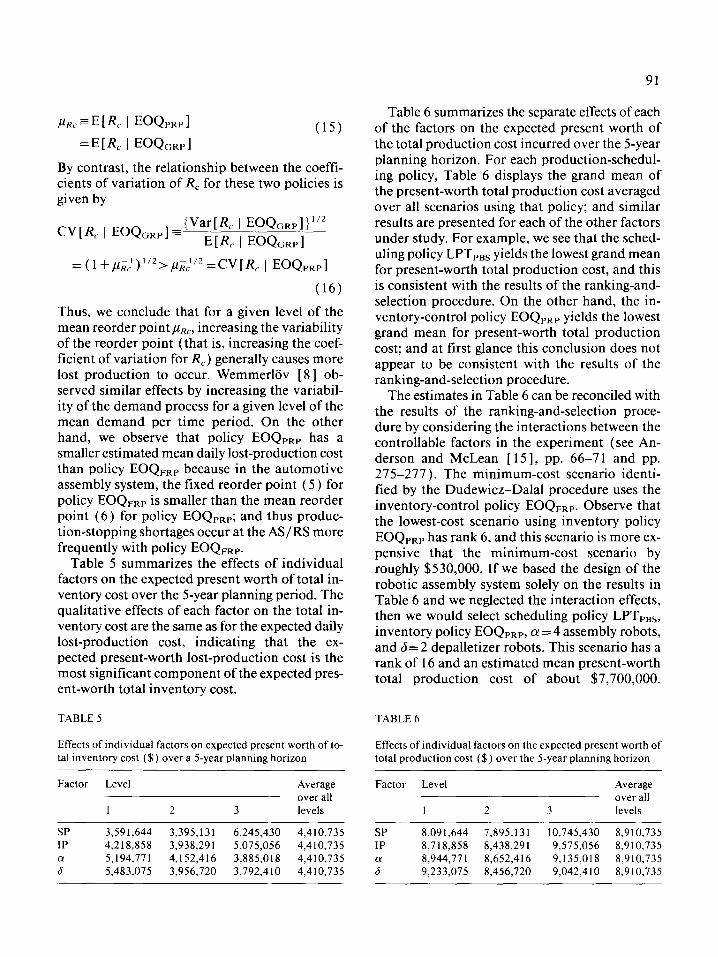
Table 5 summarizes the effects of individual factors on the expected present worth of total inventory cost over the 5-year planning period. The qualitative effects of each factor on the total inventory cost are the same as for the expected daily lost-production cost, indicating that the expected present-worth lost-production cost is the most significant component of the expected present-worth total inventory cost.

TABLE 5

Effects of individual factors on expected present worth of total inventory cost ($) over a 5-year planning horizon

Factor Level Average over all

1 2 3 levels

Table 6 summarizes the separate effects of each of the factors on the expected present worth of the total production cost incurred over the 5-year planning horizon. For each production-scheduling policy, Table 6 displays the grand mean of the present-worth total production cost averaged over all scenarios using that policy; and similar results are presented for each of the other factors under study. For example, we see that the scheduling policy LPTpBs yields the lowest grand mean for present-worth total production cost, and this is consistent with the results of the ranking-and- selection procedure. On the other hand, the inventory-control policy EOQpRp yields the lowest grand mean for present-worth total production cost; and at first glance this conclusion does not appear to be consistent with the results of the ranking-and-selection procedure.

The estimates in Table 6 can be reconciled with the results of the ranking-and-selection procedure by considering the interactions between the controllable factors in the experiment (see An- derson and McLean [ 151, pp. 66-71 and pp. 275-277). The minimum-cost scenario identified by the Dudewicz-Dalal procedure uses the inventory-control policy EOQFRP. Observe that the lowest-cost scenario using inventory policy EOQpRp has rank 6, and this scenario is more ex- pensive that the minimum-cost scenario by roughly $530,000. If we based the design of the robotic assembly system solely on the results in Table 6 and we neglected the interaction effects, then we would select scheduling policy LPTPBS, inventory policy EOQPRP, (x = 4 assembly robots, and 6= 2 depalletizer robots. This scenario has a rank of 16 and an estimated mean present-worth total production cost of about $7,700,000.

TABLE 6

Effects of individual factors on the expected present worth of total production cost ($) over the 5-year planning horizon

Factor Level Average over all

1 2 3 levels

SP 3,591,644 3,395,131 6,245,430 4,410,735 IP 4,2 18,858 3,938,291 5,075,056 4,410,735 : 5,483.075 5,194,771 4,152,416 3,885,018 4,410,735

3,956,720 3,792,410 4,410,735

SP 8,091,644 7,895,131 10,745,430 8,910,735 IP 8,718,858 8,438,291 9,575,056 8,910,735 : 8,944,771 8,652,416

9,233,075 8,456,720 9,135,018 9,042,410 8,910,735 8,910,735

92

Therefore, the cost of neglecting the interaction effects would be about $1 ,OOO,OOO.

6. Conclusions

In this paper we have presented a simulation model of an AS/RS feeding a robotic assembly system. The modeling objective was to minimize the expected present worth of total production cost incurred over the operational life of the system. Using a statistical ranking-and-selection procedure that has been adapted to discrete simulation experiments, we identified a minimum- cost system design specifying the production- scheduling policy for the assembly robots, the inventory-control policy for the AS/R& the number of assembly robots, and the number of depalletizer robots.

Even though this study was performed on a single specific system, the method of analysis detailed in this paper can be applied to any manufacturing system that is integrated with an AS/RS. Moreover, several general conclusions can be drawn from this study. (a) Frequently there exist highly significant interactions between the design factors for such manufacturing systems, and these interactions invalidate simple one-factor-at-a-time procedures for finding the minimum-cost system design. (b) In the analysis of simulation-generated responses (costs ), sub- stantial disparities between the response variances for different system configurations invalidate classical ANOVA techniques. We believe that a valid and efficient approach to the problem of selecting optimal system designs can be based on statistically designed simulation experiments using appropriate ranking-and-selection procedures that have been adapted to simulation. To screen a large number of alternatives, we recommend applying the restricted subset selection procedure of Sullivan and Wilson [ 13 ] in a pilot study so that all inferior alternatives can be quickly identified and eliminated from further consideration.

Acknowledgments

The authors thank Paul Caruso of Ford Motor Company for his helpful comments on this paper and for his support of a study that formed part of the original basis for the paper. The authors also thank Monica T. Dessouky and A. Alan B. Prit-

sker for their insightful critiques of previous ver- sions of this paper. The original study was performed by Maged Dessouky while employed at Pritsker & Associates. James Wilson’s research was partially supported by the National Science Foundation under Grant No. DMS-87 17799. The U.S. Government has certain rights in this material.

References

I

2

3

4

5

6

7

8

9

IO

II

12

13

14

15

Material Handling Institute, 1980. Considerations for

planning and installing an automated storage/retrieval

system. Technical Report, Automated Storage/Re-

trieval Systems Product Section, Pittsburgh, PA.

Tompkins, J.A. and White, J.A., 1984. Facilities Plan-

ning. John Wiley & Sons, Canada. Dessouky, M.M., 1987. Minimizing production costs for

a robotic assembly system. Unpublished M.S.I.E. The-

sis, Purdue University, West Lafayette, IN.

Caruso, P.C. and Dessouky. M.M., 1987. Analytical fac-

tors concerning the use of micro-mini storage devices as

material management systems. In: A. Thesen, H. Grant

and W. Kelton (Eds.), Proceedings of the 1987 Winter

Simulation Conference. Institute of Electrical and Elec-

tronics Engineers, Piscataway, NJ, pp. 692-696.

Conway, R.W., Maxwell. W.L. and Miller, L.W., 1967.

Theory of Scheduling. Addison-Wesley, Reading, MA.

Bruno, J., Downey, P. and Frederickson, G.N., 198 1.

Sequencing tasks with exponential service times to min-

imize the expected flow time or makespan. Journal of

the Association for Computing Machinery, 28: 100-l 13.

Wilson, R.H., 1934. A scientific routine for stock con-

trol. Harvard Business Riview, XIII.

Wemmerlov, U., 1989. The behavior of lot-sizing pro-

cedures in the presence of forecast errors. Journal of Op-

erations Management, 8: 37-47.

Haddock, J. and Hubicki, D.E., 1989. Which lot-sizing

techniques are used in material requirements planning?

Production and Inventory Management Journal, 30: 53-

56.

Pritsker, A.A.B., 1986. Introduction to Simulation and

SLAM II. John Wiley & Sons, New York, 3rd edn.

Welch, P.D., 1983. The statistical analysis of simulation

results. In: S.S. Lavenberg (Ed.), Computer Perform-

ance Modeling Handbook. Academic Press, New York,

pp. 267-329. Dudewicz, E.J. and Dalal, S.R., 1975. Allocation of observations in ranking and selection with unequal vari-

ances. Sankhya. B-37: 28-78.

Sullivan, D.W. and Wilson. J.R., 1989. Restricted subset selection procedures for simulation. Operations Re-

search, 37: 52-7 1.

Law, A.M. and Kelton, W.D., 1982. Simulation Model-

ing and Analysis. McGraw-Hill, New York.

Anderson, V.L. and McLean, R.A., 1974. Design of Ex-

periments: A Realistic Approach. Marcel Dekker, New York.

Documents

Minimizing production costs for a robotic assembly systemmaged/publications/Minimizing Production Costs.pdf · Minimizing production costs for a robotic assembly system ... School