The Response of Private Consumption to Different Public Spending Categories: VAR Evidence from UK

Luigi Marattin± Simone Salotti÷

(University of Bologna) (University of Siena)

Abstract This paper performs a Structural VAR analysis on UK economy using quarterly non-interpolated data from 1981 to 2005 in the attempt to verify and quantify private consumption’s response to different components of public expenditure (government consumption, social spending and wage component). Our findings suggest that any empirical support of competing theoretical models on the issue would probably benefit from a disaggregation of government expenditure, rather than focusing on the aggregate measure. In fact, while shocks to pure government consumption trigger a RBC-like reduction in private consumption, shocks to the non-systematic component of social spending generate positive reaction, in line with the “credit-constrained-agents” approach. The cumulative impact on GDP after three years of a government spending shock (close to a negative 1% of GDP) is twice as much the social spending shock, with opposite sign. Government wage shocks do not seem to have any significant effects on private consumption. Public expenditure composition, rather than level, seems to be actually playing the most crucial role when it comes to aggregate demand support via effects on private consumption.

JEL classification: E62, H30. Keywords: Fiscal policy, government expenditure, VAR analysis.

± luigi.marattin@unibo.it Department of Economics – University of Bologna – Strada Maggiore 45 – 40125 – Bologna (Italy) – Tel: +39 – 051-2092606 ÷ salotti@unisi.it Department of Economics – University of Siena – P.zza San Francesco 7 – 53100 – Siena (Italy)

1

1. Introduction The severity of the last economic downturn following the global financial crisis has intensified the

search for the typology of public expenditure able to maximize the short-term impact on economic

activity. As recovery plans’ specifications differ across countries, the very basic question remained the

same: which fiscal policy weapon is associated with the highest multiplier? The attempt to evaluate the

fiscal policy’s effectiveness has often resulted on the sign and magnitude of (actual or cyclically-

adjusted) budget deficit’s impact on GDP. Perotti (2007) provides a good review on the comparison

between different theoretical models and their empirical predictions regarding the impact on income. In

this paper, we investigate a slightly different question: how do different categories of public

expenditure affect private consumption?

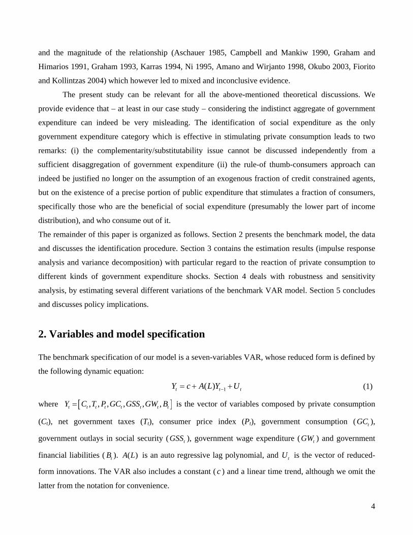
The relevance of the issue rests on private consumption’s major weight among aggregate demand’s

components, as showed by Figure 1. This in turn is the reason why consumption’s response to

economic stimulus plans is the key determinant of output multipliers.

FIGURE 1 ABOUT HERE

In order to answer this question, we perform a structural VAR analysis on the UK economy, using

quarterly non-interpolated data from 1981 to 2005. In line with some recent studies (Beetsma et al.

2006, Beetsma 2008, Giordano et al. 2007, Cavallo 2005 and 2007, Monacelli and Perotti 2008) we do

not focus on public finance aggregates but rather on budget deficit’s single components. Our

disaggregation is mainly on the expenditure side, as we are primarily concerned with the aggregate

consumption effects of different public expenditure categories. Unlike many of the above-mentioned

contributions, we do not limit ourselves to the identification of wage and non-wage components of

public expenditure, but rather distinguish among government consumption, government wage

expenditure and social spending.

Our results, robust to a number of alternative specifications, show that the only component

resulting in a positive and significant response of private consumption is social expenditure, defined as

the sum of social security benefits and subsidies, net of social security contributions. On the other hand,

government consumption seems to have a negative and significant effect, whereas wage expenditure

has no impact. Regarding the magnitude of those effects, in our benchmark model the cumulative

impact on private consumption of a government spending shock equal to 1% of GDP is in absolute

2

terms higher than the one (of the same magnitude) to the social expenditure component: while shocks

to the former lead to a -0.9% impact on GDP, shocks to the latter cause a +0.5% cumulative response.

A consequence of our analysis is that using total government expenditure (by aggregating the three

components above) does not seem to be a reasonable simplification: in fact, when these three

components of government expenditure enter the VAR in a unique aggregate measure, the result is a

zero-impact on private consumption (see section 4), as also found by Perotti (2004)1. Instead,

disaggregating public expenditure conveys more detailed and differentiated information on its actual

capabilities to affect private consumption.

We believe these results to be relevant for the theoretical debate between alternative and

competing approaches modelling private consumption’s impact of fiscal shocks. As it is well known,

the standard neoclassical RBC model predicts a fall in consumption following a government

expenditure shock, because of the Ricardian equivalence: higher public spending must be matched by

an equivalent increase in taxation in present discounted terms, therefore intertemporal optimizing

consumers suffer from a negative wealth effect that decreases consumption. Effects on output are

positive due to increased labor supply, triggered by the wealth effect. Since virtually no study seems to

confirm the prediction of the standard neoclassical model (as pointed out by Galì, Lopez-Salido and

Valles 2007), New Keynesian tradition attempted to reconcile theory with empirical evidence and

rescued a consumption-enhancing role for fiscal policy. This has been accomplished either using finite-

horizons frameworks (Blanchard 1985) or introducing credit-constrained agents and rule-of-thumb

consumers (Mankiw, 2000, Galì et al 2004, 2007)2. This latter approach has particularly gained

considerable attention. It includes a fraction of non-Ricardian households who do not optimize over the

life cycle and are thus forced to consume out of current income, so that their consumption responds

promptly to a fiscal policy impulse3. A further research strand explicitly considers the per se

government expenditure’s impact on consumption. This is often carried out by an ad-hoc utility

function specification where private and public consumption are entered in a non-additive form, so to

obtain a non-zero impact of one on the marginal utility of the other (Bouakez and Rebei 2003, Marattin

2008); on the other hand, there is a large non-VAR empirical literature attempting to assess the sign

1 Perotti finds a non-significant effect of fiscal shocks on consumption for the period 1980-2000. We confirm this finding, with an aggregate measure of consumption, over a 1981 – 2005 sample. 2 As a matter of fact, there is also a third way to the same result. Ravn et al. (2004) obtain a positive effect on consumption with credit-constrained agents, but assuming that the representative individual forms consumption habits on the individual variety in a monopolistic competition setting, rather than on aggregate consumption. 3 As discussed by Galì, Lopez-Salido and Valles (2007), the presence of non-Ricardian consumers must be coupled with sticky prices and imperfectly competitive markets in order to obtain a private consumption’s positive response.

3

and the magnitude of the relationship (Aschauer 1985, Campbell and Mankiw 1990, Graham and

Himarios 1991, Graham 1993, Karras 1994, Ni 1995, Amano and Wirjanto 1998, Okubo 2003, Fiorito

and Kollintzas 2004) which however led to mixed and inconclusive evidence.

The present study can be relevant for all the above-mentioned theoretical discussions. We

provide evidence that – at least in our case study – considering the indistinct aggregate of government

expenditure can indeed be very misleading. The identification of social expenditure as the only

government expenditure category which is effective in stimulating private consumption leads to two

remarks: (i) the complementarity/substitutability issue cannot be discussed independently from a

sufficient disaggregation of government expenditure (ii) the rule-of thumb-consumers approach can

indeed be justified no longer on the assumption of an exogenous fraction of credit constrained agents,

but on the existence of a precise portion of public expenditure that stimulates a fraction of consumers,

specifically those who are the beneficial of social expenditure (presumably the lower part of income

distribution), and who consume out of it.

The remainder of this paper is organized as follows. Section 2 presents the benchmark model, the data

and discusses the identification procedure. Section 3 contains the estimation results (impulse response

analysis and variance decomposition) with particular regard to the reaction of private consumption to

different kinds of government expenditure shocks. Section 4 deals with robustness and sensitivity

analysis, by estimating several different variations of the benchmark VAR model. Section 5 concludes

and discusses policy implications.

2. Variables and model specification The benchmark specification of our model is a seven-variables VAR, whose reduced form is defined by

the following dynamic equation:

1( )t tY c A L Y U− t= + + (1)

where [ ], , , , , ,t t t t t t tY C T P GC GSS GW B= t is the vector of variables composed by private consumption

(Ct), net government taxes (Tt), consumer price index (Pt), government consumption ( ),

government outlays in social security ( ), government wage expenditure ( ) and government

financial liabilities (

tGC

tGSS tGW

tB ). ( )A L is an auto regressive lag polynomial, and is the vector of reduced-

form innovations. The VAR also includes a constant ( ) and a linear time trend, although we omit the

latter from the notation for convenience.

tU

c

4

“The availability of quarterly fiscal variables represents the main constraint for the analysis of fiscal

policy with VAR models” (Giordano et al. 2008, p. 6). Furthermore, Perotti (2004) correctly warns

against the distortions coming from the usage of quarterly data set obtained by interpolation of yearly

values. This remark makes the data availability constraint even more binding, and poses considerable

limitations to the implementation of a fully-equipped large scale time series analysis. We have chosen

to sacrifice the generality of our conclusions in favour of a complete non-interpolated quarterly data

set; this paper focuses on United Kingdom, and uses data from 1981Q1 to 2005Q44.

The source for almost all of the variables that we used is the OECD Economic Outlook No 835.

The benchmark specification includes: the log of real private final consumption expenditure per capita

C, the log of real taxes per capita T (defined as the sum of direct and indirect taxes, other receipts and

property income received by government), the harmonized consumer price index P6, the log of real

government consumption per capita GC (defined as the sum of government final non-wage expenditure

and other current outlays), the log of real government social expenditure per capita GSS (defined as the

sum of net social security benefits and subsidies), the log of real government final wage expenditure

per capita GW, the log of real government financial liabilities per capita B. Additional variables used

for robustness checks include the log of real GDP per capita, the short term interest rate on government

bonds, and the sum of the three components of government expenditure, GTOT. All real variables are

deflated by the GDP deflator. Population data come from the World Development Indicators of the

World Bank.

We estimate the seven equations of system (1) independently using least squares. The number

of lags is set to five according to the Akaike Information Criterion and the absence of serial correlation

in the residuals, positively checked with a Lagrange Multiplier test7. Moreover, we failed to reject the

hypothesis of normality of residuals with the Jarque-Bera statistics and we checked the stability

condition of the VAR, finding that all eigenvalues comfortably lie inside the unit circle. We also tested

for the presence of cointegrating relationships among the variables, finding mixed evidence according

to the rank and the maximum eigenvalue tests. Due to that, and given that our a priori did not include a

meaningful long-run relationship among the variables, we decided not to impose any cointegrating

4 This period has been chosen because of the strong evidence that points towards a structural break between 1981 and the previous period (Perotti, 2004). 5 The quarterly data of the Economic Outlook are normally obtained by interpolation, but not those of the UK. 6 Here the source is UK National Statistics. 7 The chi-square statistics for autocorrelation up to first and second order and 2 are 54.0872 and 33.7088 which imply p-values, respectively, of 0.2863 and 0.9528. Different criteria for lag length selection (final prediction error, AIC, SIC) led to

5

restriction and, thus, estimate the VAR with the variables in levels (Sims et al. 1990, Giordano et al.

2008).

We turn now to the identification issue. The literature on fiscal policy VARs has traditionally

adopted two alternative strategies in order to identify exogenous and unexpected fiscal shocks

(Beetsma, 2008). The first one identifies deviations of fiscal policy from its systematic path by using

dummy variables so to capture specific episodes that can reasonably be interpreted as exogenous and

unforeseen (Ramsey and Shapiro 1999, Burnside et al 2004, Romer and Romer 2007, Monacelli and

Perotti 2008). Such a strategy has the advantage of being simple and straightforward, as it is relatively

easy to justify and does not require any additional assumption; on the other hand, it might lack the

appropriate accuracy, since the resulting impulse response functions might be affected by the delayed

effects of previous events who are not captured by the contemporaneous effect of the dummy. The

second strategy – more widespread - imposes alternative types of structural restrictions: they can be

sign restrictions on the impulse response functions (Uhlig 2005, Mountford and Uhlig 2005, Canova

and Pappa 2007,Enders et al 2008), external and institutional information exploiting the quarterly

nature of data and fiscal policy decision lags (Blanchard and Perotti 2002, Perotti 2004, Muller 2008,

Monacelli and Perotti 2008), or restrictions on contemporaneous relations among variables and error

terms in the structural form (Marcellino 2006, Beetsma et al 2006, Beetsma 2008, Benetrix and Lane

2009).

Our identification strategy is the latter. In particular, we adopt a Cholesky factorization so to

recover the vector of structural shocks tε (and its variance Ω ) from the reduced-form error in (1),

according to the following scheme:

tU

(2)

10 10 0 10 0 0 10 0 0 0 10 0 0 0 0 10 0 0 0 0 0 1

C CC C C C C Ct t

T P GC GSS GW BT T

T T T T Tt tP GC GSS GW B

P PP P P Pt tGC GSS GW BGC GCGC GC GC

t tGSS GW BSS GSSGSS

GW BtGWGW

BtB

t

u

u

u

u

u

ε α α α α α αε α α α α αε α α α αε α α α

α αεαε

ε

⎡ ⎤ ⎛ ⎞⎢ ⎥ ⎜ ⎟⎢ ⎥ ⎜ ⎟⎢ ⎥ ⎜ ⎟⎢ ⎥ ⎜ ⎟⎢ ⎥ = ⎜ ⎟⎢ ⎥ ⎜ ⎟⎢ ⎥ ⎜ ⎟⎢ ⎥ ⎜ ⎟⎢ ⎥ ⎜ ⎟⎢ ⎥ ⎝ ⎠⎣ ⎦

GSSt

GWtB

t

u

u

⎡ ⎤⎢ ⎥⎢ ⎥⎢ ⎥⎢ ⎥⎢ ⎥⎢⎢ ⎥⎢ ⎥⎢ ⎥⎢ ⎥⎣ ⎦

⎥

The Cholesky ordering as in (2) is equivalent to assuming the following set of conditions. Consumption

a number of lags smaller than three, but dealing with quarterly data on fiscal policy we decided to disregard these options as

6

is the most endogenous variable and it is therefore affected by all contemporaneous values of all the

variables of the VAR; this is natural, as the present study is primarily concerned with the analysis of

macroeconomic effects on private consumption. Tax revenue is allowed to depend on prices and all

fiscal variables, assuming that the government operates under a balanced budget-like stance8. Nominal

rigidities in the form of delayed price adjustments justify the fact that the general price index is not

affected by demand conditions within the quarter. Fiscal variables are modelled as the most exogenous

ones, starting from the real stock of government liabilities, which can legitimately be considered as

given in a quarterly data set; government wage expenditure is assumed to be the most rigid among

spending categories, as its dynamics are usually governed by collective contracts whose length is well

beyond the quarter. Social expenditure and government purchases of goods and services are thought to

be featured by lower degrees of exogeneity in the ordering. Note that all government expenditure

categories are allowed to depend on debt. Although our scheme can be arguable (as it is often the case

in a Cholesky ordering), we believe that the data frequency grants us a sufficient degree of flexibility in

the choice; we also provide a number of robustness checks in section 5 so to strengthen the general

validity of our benchmark estimation.

3. Estimation results 3.1 Impulse response analysis

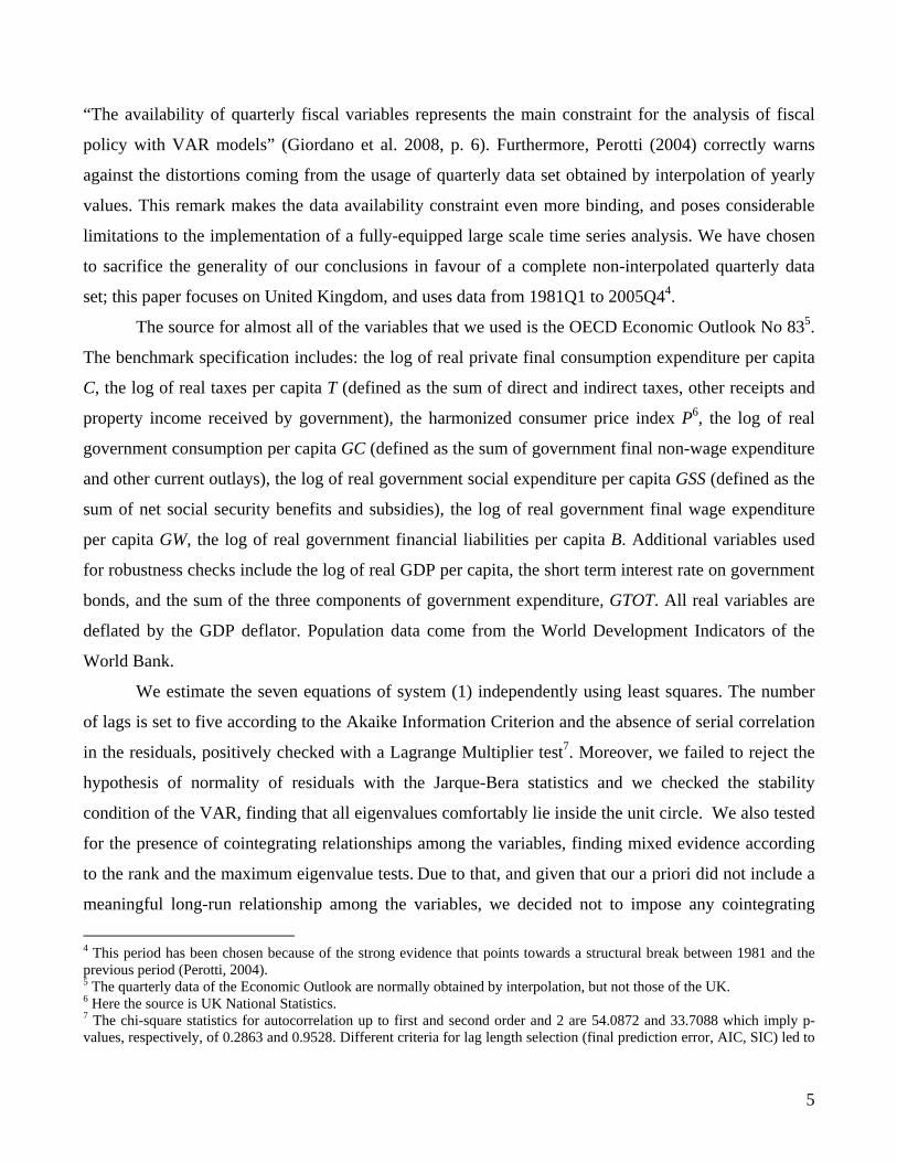
Figures 2a-c display the results of our baseline model.

FIGURE 2a, 2b, 2c ABOUT HERE

Each figure displays the response of all the 7 variables of the model to each one of the three

government spending variables shocks equal to 1 percent of GDP (Figures 2a, 2b and 2c display the

responses to shocks in GC, GSS and GW respectively). In order to derive the 16th and 84th percentiles

of the impulse-response distribution in the figures, we perform Monte Carlo simulations and assume

normality in the parameter distribution. Based on that information, we construct t-tests based on 1000

different responses generated by simulations, and check whether the point estimates of the mean

impulse-responses are statistically different from zero. The responses of private consumption are

we preferred to include at least one year of observations. 8 Automatic effects of VAT taxation within the quarter are neglected.

7

expressed as shares of GDP by multiplying the response from the VAR (which is expressed in logs) by

the sample average share of private consumption in GDP (as in Monacelli and Perotti, 2006).

Notice, first, that shocks in government consumption and in social spending lead to opposite effects on

private consumption: while the first depresses it, as predicted by neoclassical models, the second

increases it, as assumed by the New Keynesian approach. Both responses are statistically significant at

conventional levels, as shown in Tables 1a-c. Both shocks are very persistent, even though the effects

are perceived after three and five quarters in case of, respectively, government consumption and social

spending. The former reaches the peak after 9 quarters, with a cumulative (negative) impact of -0.7%

of GDP; the latter after 10 quarters, with a cumulative (positive) impact of 0.4%. It is interesting to

note that the cumulative impact after three years of a government spending shock is approximately

double the one of social spending, with reversed signs: shocks to government consumption lead to a -

0.9% reduction in GDP, whereas shocks to social spending cause a +0.5% cumulative output response.

On the other hand, shocks in government wage expenditure have no significant effects on consumption.

It is worth mentioning the fact that a shock in net taxes seems to affect positively consumption, thereby

implying a Ricardian effect of tax-based fiscal consolidation - but the effects are not statistically

different from zero at conventional levels.

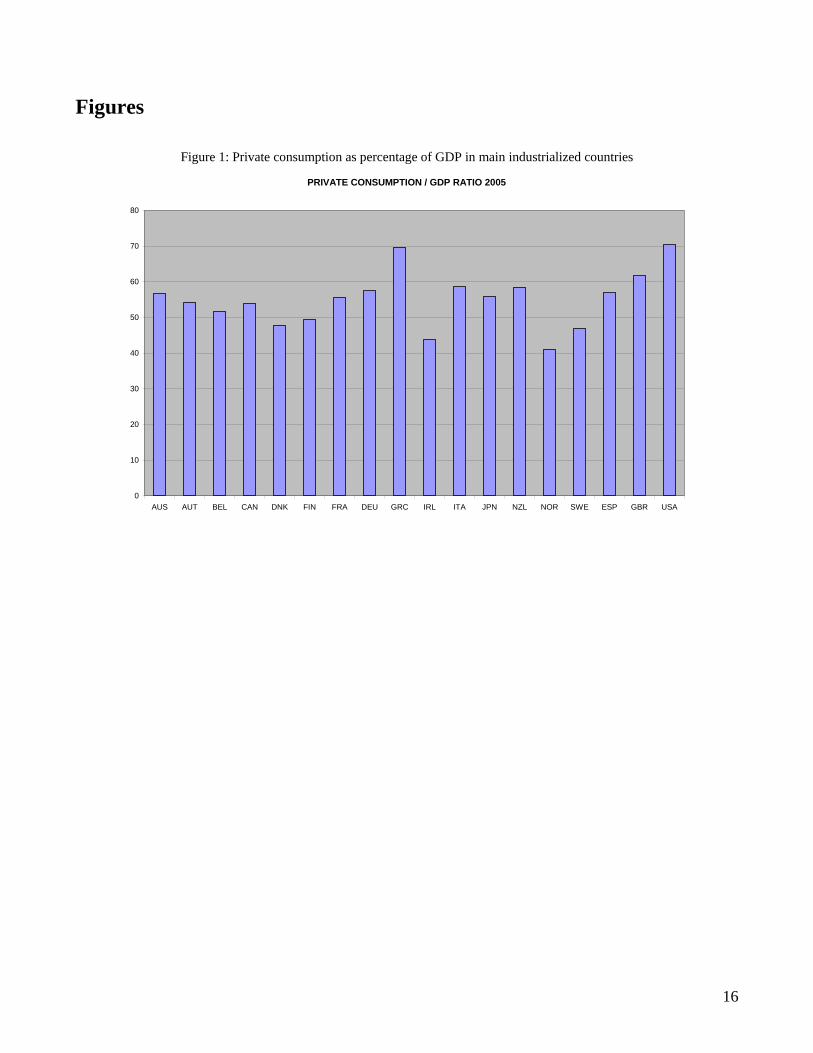
3.2 Variance Decomposition

The variance decomposition analysis is complementary to the impulse response analysis presented

above, since it is informative on the relative power of each shock in explaining the forecast error

variance of the VAR equations at different forecast horizons. In particular, we look at the contribution

of innovations in the three components of government spending to the forecast error variance of the

private consumption equation.

FIGURE 3 ABOUT HERE

Figure 3 shows that, consistently with the impulse response analysis, the proportion of the forecast

error variance in the private consumption equation explained by government consumption and social

spending is considerably larger than the one explained by the wage expenditure. Moreover, government

consumption and social spending have a similar importance in explaining the variance of private

consumption (they are both slightly below 20% after 15 periods). Finally, note that the forecast error

variance attributable to the 3 components of government expenditure overwhelms even the variance

8

attributable to private consumption itself after 10 periods. This is a confirmation of the importance of

the role played by fiscal policy innovations in determining private consumption’s dynamics.

4. Robustness In order to check the robustness of our results, we estimated several different VARs to verify whether

baseline model’s response of private consumption to shocks in the government expenditure variables

are confirmed within alternative specifications. Our robustness check proceeds along three steps.

The first one is made of three slight modifications of the baseline model. First we exclude the time

trend from the estimation; then we add quarterly dummies, as conventional in the literature (Monacelli

and Perotti 2006); finally we include (along with the time trend and seasonal dummies) an additional

dummy accounting for Labour party terms in office (specifically, since 1997Q2). The motivation for

this test lies in the nature of the relationship this paper investigates: given the non-negligible

differences in the stance towards government expenditure by Conservative and Labour governments,

we wanted to check whether any differences can be observed in the empirical analysis.

Figures 4, 5 and 6 show, respectively, impulse response functions related to the three above

specifications of our first robustness step.

FIGURE 4, 5, 6 ABOUT HERE

As it can be easily seen, our results are robust – in terms of significance and sign of responses - to

these changes to the baseline model (Table 2, 3 and 4 in the Appendix contains the details of the

responses).

The second step includes the variation of the VAR dimension and/or variables. Again, the

results hold across these different specifications. Figure 7 (with details in Table 5 in the Appendix)

shows the results of a 7-variables VAR with the short term interest rate in place of government

financial liabilities (this alternative variable is taken into account in various previous studies, such as

Marcellino 2006 and Monacelli and Perotti 2007). Figure 8 (and Table 6) displays the result of a 7-

variables VAR containing the log of real GDP per capita instead of the price index from the baseline

model.

FIGURE 7 AND 8 ABOUT HERE

9

Figure 9,10 and 11 (and Tables 7-9) show the results of three 6-variables VARs resulting from the

exclusion of, respectively, financial liabilities, net taxes and the price index. Once more, the negative

effects of a government consumption shock and the positive effects of shocks in social spending are

well supported by the data.

FIGURE 9,10 AND 11 ABOUT HERE

As final exercise of this second step, we estimate a more parsimonious 5-variables VAR containing

consumption, price index and the three components of government expenditure. Results in Figure 12

(and Table 10) are again confirmed.

FIGURE 12 ABOUT HERE

Our third and final step is maybe the most relevant. We estimate four 5-variables VARs where,

compared to the baseline model, each government expenditure category is included separately as the

only component; finally, we estimate a specification where we recompose our disaggregation by

including the total aggregate expenditure (GTOT) obtained by summing up the three components that

we analysed separately so far9.

FIGURE 13 ABOUT HERE

Figure 13 presents the impulse response functions of our third robustness step. In particular, we

can notice that the effects of total government expenditure shocks on consumption are not significantly

different from zero, thereby pointing to a general ineffectiveness of public spending in stimulating

private consumption. However, each component has a different quantitative and qualitative impact on

consumption, and results are the same as in our benchmark 7-variables model and throughout the

robustness checks. A general point can be made about the lagged response of private consumption to

GC and GSS, that we observe in virtually all our estimates: while the (negative) effect of the former is

significant pretty soon after the shock, the (positive) effect of social spending becomes statistically

significant later (after 5/6 quarters). This result might suggest a tempting interpretation, based on the

10

theoretical debate we base our empirical analysis upon. Since credit-constrained agents consume out of

the social expenditure they benefit from, it is plausible to observe a time lag between the moment when

the spending decision is approved (when we observe the public expenditure shock), and the moment

when the agents’ disposable income is actually affected (when private consumption reacts). On the

other hand, the quicker (negative) response to government consumption might suggest a RBC-like

anticipation effect: the mere approval of an increase in that component triggers a reduction in private

consumption, following the negative wealth effect.

5. Conclusions This paper carried out an empirical analysis on UK economy using quarterly non-interpolated data

from 1981 to 2005. Our objective was to verify and quantify the effects of different broad categories of

government expenditure on private consumption. Our findings, robust to a number of alternative

specifications of the SVAR, can be summarized as follows. Private consumption seems to respond: i)

negatively to government purchases of goods and services; ii) positively on social spending; iii) not

significantly to government wage expenditure. While i) seems to confirm the standard neoclassical

wealth effect, ii) strengthens the competing theoretical approach, known as the “credit-constrained”

agents (who, in our interpretation, can be identified as the individuals social expenditure is targeted to,

as it provides them with the resources to consume out of). Quantitative estimates of the responses’

magnitude in our benchmark specification lead to an important policy implication: shocks to

government consumption have a cumulative impact on GDP after three years – via private consumption

- that is twice as much the one of social spending, with opposite signs. This suggests that any

expansionary effect of social expenditure might be potentially offset by a parallel increase in pure

government consumption, with a negative effect on aggregate demand even though a overall increase

in aggregate government expenditure has occurred. This result is strengthened by our robustness tests,

showing that trying to measure the fiscal multiplier on private consumption by considering the whole

government expenditure aggregate – and not its decomposition according to features and goals – can

indeed be misleading.

While we believe that this analysis can represent a useful contribution to a more effective management

of fiscal policy tools on the expenditure side, the general validity of the findings is certainly limited by

the closed-economy one-country investigation. A panel-VAR analysis on EMU countries would permit

9 Note that this aggregate variable adds up exactly to government expenditure net of debt service payments.

11

the use of easily-available annual data, allowing a more complete answer to our original question,

would probably be the most rationale next step.

12

References Amano, R. A. and Wirjanto T. S. (1997), "Intertemporal Substitution and Government Spending" The

Review of Economics and Statistics 1, 605-09.

Ashauer, D. (1985), "Fiscal Policy and Aggregate Demand" American Economic Review, 75 (1) 117-

127.

Beetsma, R., Giuliodori M. and Klaassen, F. (2006), “Trade Spill-Overs of Fiscal Policy in the

European Union: A Panel Analysis” Economic Policy 21 (48): 639-687.

Beetsma, R. (2008), “A Survey of the Effects of Discretionary Policy” Working paper, University of

Amsterdam, Amsterdam School of Economics.

Benetrix, A. and Lane, P. (2009), “Fiscal Shokcs and the Real Exchange Rate” IIIS Discussion Paper

No.286.

Blanchard, O.(1985) "Debt, Deficits and Finite Horizons" Journal of Political Economy, Vol.93,No.2,

223-247.

Blanchard, O. and Perotti, R. (2002), "An Empirical Characterisation of the Dynamic Effects of

Changes in Government Spending and Taxes on Output" Quarterly Journal of Economics,

vol.117(4),p.1329-1368.

Bouakez, H, Rebei, N. (2003), "Why Does Private Consumption Rises After a Government Spending

Shock?" Bank of Canada Research Paper.

Burnside, C., Eichenbaum, M. and Fisher, J. (2004), “Fiscal Shocks and Their Consequences”, Journal

of Economic Theory 115 (1): 89-117.

Campbell, J. Y. and Mankiw, G. W. (1990), "Permanent Income, Current Income and Consumption"

Journal of Business and Economic Statistics 8, 265-279.

Canova, F. and Pappa, E. (2007), “Price Differentials in Monetary Unions: The Role of Fiscal Shocks”

, Economic Journal 117: 713-737.

Cavallo, M. (2005), “Government Employment Expenditure and the Effects of Fiscal Policy Shocks”

Working paper 16, Federal Reserve Bank of San Francisco.

Cavallo, M. (2007), “Government Consumption Expenditure and the Current Account”, Public Finance

and Management 7: 73-115.

Enders Z., Muller, G. and Scholl, A. (2008), “How Do Fiscal and Technology Shocks Affect Real

Exchange Rates? New Evidence for the United States”, Center of Financial Studies No.2008/22.

Favero, C. and Giavazzi, F. (2007), "Debt and the Effects of Fiscal Policy", NBER working paper

no.12221.

13

Fiorito, R. and Kollintzas, T. (2004), "Public Goods, Merit Goods and the Relation between Private and

Government Consumption" European Economic Review 48 1367-1398.

Gali, J., Lopez-Salido, J. D and Valles, J. (2004), "Rule-of-Thumb Consumers and the Design of

Interest Rate Rules", Journal of Money, Credit and Banking, Vol.36 (4), 739-764.

Gali, J., Lopez-Salido, J. D. and Valles, J. (2007), "2007), "Understanding the Effect of Public

Spending on Consumption",Journal of the European Economic Association 5(1):227-270.

Giordano, R., Momigliano S., Neri, S. and Perotti, R. (2007), “The Effects of Fiscal Policy in Italy:

Evidence from a VAR Model”, European Journal of Political Economy 23 (3),: 707-733.

Graham, F. C., (1993), "Fiscal Policy and Aggregate Demand : Comment" American Economic Review

83,659-666.

Graham, F. C and Himarios, D. (1991), "Fiscal Policy and Private Consumption: Instrumental

Variables Tests of the Consolidation Approach" Journal of Money, Credit and Banking 23 (1), 53-

67.

Karras,G., "Government Spending and Private Consumption: Some International Evidence" Journal of

Money, Credit and Banking 26,9-22.

Okubo, M.(2003), Intratemporal Substitution between Private and Government Consumption: the Case

of Japan" Economics Letters 79: 75-81

Mankiw, N.G., (2000), “The Savers-Spenders Theory of Fiscal Policy”, American Economic Review,

90, 120-125.

Marattin, L. (2008), "Private and Public Consumption and Counter-Cyclical Fiscal Policy"

International Journal of Economics, Vol.2, Issue 1.

Marcellino, M. (2006), “Some Styilized Facts on Non-Systematic Fiscal Policy in the Euro Area”,

Journal of Macroeconomics 28, 461-479.

Monacelli, T. and Perotti, R. (2008), “Openness and the Sectoral Effects of Fiscal Policy”, Journal of

the European Economic Association 6 (2.3): 395-403

Mountford, A. and Uhlig, H. (2005), “What Are the Effets of Fiscal Policy Shocks?” , SFB 649

Discussion Papers SFV649DP2005-039, Sonderforschungsbereich 649, Humboldt University, Berlin,

Germany.

Muller, G. (2008), “Understanding the Dynamic Effects of Government Spending on Foreign Trade”,

Journal of International Money and Finance 27 (3), 345-371.

Ni, S. (1995),"An Empirical Analysis on the Substitutability between Private Consumption and

Government Purchases",Journal of Monetary Economics 36, 593-605.

14

Perotti, R. (2004), “Estimating the Effects of Fiscal Policy on OECD Countries,” Working Paper,

IGIER-Bocconi.

Perotti, R. (2007), "In Search of the Transmission Mechanism of Fiscal Policy", NBER working paper

no.13143.

Ramsey, V. and Shapiro, M. (1999), “Costly Capital Reallocation and the Effects of Government

Spending” , Carnegie-Rochester Conference Series on Public Policy 48:145-194.

Ravn, M., Schmitt-Grohè, S. and Uribe, M. (2004), “Deep Habits,“ Review of Economic Studies, 73,

pp. 195-218.

Romer, C. and Romer, D. (2007), “The Macroeconomic Effects of Tax Changes: Estimates Based on a

New Measure of Fiscal Shocks”, Working paper, University of California, Berkeley.

Sims, C, Stock, J. and Watson, M. (1990), “Inference in Linear Time Series Models with Some Unit

Roots”, Econometrica, 58, 113-44.

Uhlig, H., (2005), “What Are the Effects of Monetary Policy on Output? Results from An Agnostic

Identification Procedure”, Journal of Monetary Economics 52 (2), 381-419.

15

Figures

Figure 1: Private consumption as percentage of GDP in main industrialized countries

PRIVATE CONSUMPTION / GDP RATIO 2005

0

10

20

30

40

50

60

70

80

AUS AUT BEL CAN DNK FIN FRA DEU GRC IRL ITA JPN NZL NOR SWE ESP GBR USA

16

Figure 2a: responses of all variables to a shock of GC

-0.4

0.0

0.4

0.8

1.2

1.6

0 2 4 6 8 10 12 14

B

-.16

-.12

-.08

-.04

.00

.04

0 2 4 6 8 10 12 14

C

0.0

0.2

0.4

0.6

0.8

1.0

1.2

0 2 4 6 8 10 12 14

GC

-.4

-.2

.0

.2

.4

.6

.8

0 2 4 6 8 10 12 14

GSS

-.1

.0

.1

.2

.3

.4

0 2 4 6 8 10 12 14

GW

-12

-8

-4

0

4

8

0 2 4 6 8 10 12 14

P

-.16

-.12

-.08

-.04

.00

.04

.08

.12

.16

0 2 4 6 8 10 12 14

T

17

Figure 2b: responses of all variables to a shock of GSS

-1.0

-0.8

-0.6

-0.4

-0.2

0.0

0.2

0.4

0.6

0 2 4 6 8 10 12 14

B

-.02

.00

.02

.04

.06

.08

.10

0 2 4 6 8 10 12 14

C

-.2

-.1

.0

.1

.2

.3

0 2 4 6 8 10 12 14

GC

-0.8

-0.4

0.0

0.4

0.8

1.2

0 2 4 6 8 10 12 14

GSS

-.10

-.05

.00

.05

.10

.15

.20

0 2 4 6 8 10 12 14

GW

-8

-6

-4

-2

0

2

4

0 2 4 6 8 10 12 14

P

-.20

-.15

-.10

-.05

.00

.05

.10

.15

0 2 4 6 8 10 12 14

T

18

Figure 2c: responses of all variables to a shock of GW

-2.8

-2.4

-2.0

-1.6

-1.2

-0.8

-0.4

0.0

0.4

0 2 4 6 8 10 12 14

B

-.05

.00

.05

.10

.15

.20

0 2 4 6 8 10 12 14

C

-1.2

-1.0

-0.8

-0.6

-0.4

-0.2

0.0

0.2

0 2 4 6 8 10 12 14

GC

-2.0

-1.6

-1.2

-0.8

-0.4

0.0

0.4

0.8

0 2 4 6 8 10 12 14

GSS

-0.4

-0.2

0.0

0.2

0.4

0.6

0.8

1.0

1.2

0 2 4 6 8 10 12 14

GW

-20

-15

-10

-5

0

5

10

0 2 4 6 8 10 12 14

P

-.1

.0

.1

.2

.3

.4

0 2 4 6 8 10 12 14

T

19

Figure 3: forecast error variance decomposition, private consumption

0

.5

1

0 5 10 15step

C -> C

0

.01

.02

.03

.04

0 5 10 15step

T -> C

0

.1

.2

.3

0 5 10 15step

P -> C

0

.1

.2

0 5 10 15step

GC -> C

0

.05

.1

.15

.2

0 5 10 15step

GSS -> C

0

.02

.04

.06

0 5 10 15step

GW -> C

0

.05

.1

0 5 10 15step

B -> C

20

Figure 4: consumption responses, baseline model without the time trend

-.12

-.08

-.04

.00

.04

.08

0 2 4 6 8 10 12 14

GC

-.02

.00

.02

.04

.06

.08

.10

0 2 4 6 8 10 12 14

GSS

-.08

-.04

.00

.04

.08

.12

.16

.20

0 2 4 6 8 10 12 14

GW

21

Figure 5: consumption responses, baseline model with quarterly dummies

-.20

-.16

-.12

-.08

-.04

.00

.04

0 2 4 6 8 10 12 14

GC

-.02

.00

.02

.04

.06

.08

.10

0 2 4 6 8 10 12 14

GSS

-.05

.00

.05

.10

.15

.20

0 2 4 6 8 10 12 14

GW

22

Figure 6: consumption responses, baseline model with quarterly dummies, trend and Labour dummy

-.20

-.16

-.12

-.08

-.04

.00

.04

0 2 4 6 8 10 12 14

GC

-.02

.00

.02

.04

.06

.08

.10

0 2 4 6 8 10 12 14

GSS

-.05

.00

.05

.10

.15

.20

0 2 4 6 8 10 12 14

GW

23

Figure 7: consumption responses, 7-variables VAR with the short term interest rate

-.16

-.12

-.08

-.04

.00

.04

0 2 4 6 8 10 12 14

GC

-.02

.00

.02

.04

.06

.08

.10

0 2 4 6 8 10 12 14

GSS

-.10

-.05

.00

.05

.10

.15

.20

.25

0 2 4 6 8 10 12 14

GW

24

Figure 8: consumption responses, 7-variables VAR with GDP

-.16

-.12

-.08

-.04

.00

.04

.08

0 2 4 6 8 10 12 14

GC

-.02

.00

.02

.04

.06

.08

.10

.12

0 2 4 6 8 10 12 14

GSS

-.10

-.05

.00

.05

.10

.15

.20

.25

0 2 4 6 8 10 12 14

GW

25

Figure 9: consumption responses, 6-variables VAR (no financial liabilities)

-.16

-.12

-.08

-.04

.00

.04

0 2 4 6 8 10 12 14

GC

-.02

.00

.02

.04

.06

.08

.10

0 2 4 6 8 10 12 14

GSS

-.10

-.05

.00

.05

.10

.15

.20

.25

0 2 4 6 8 10 12 14

GW

26

Figure 10: consumption responses, 6-variables VAR (no net taxes)

-.16

-.12

-.08

-.04

.00

.04

0 2 4 6 8 10 12 14

GC

-.01

.00

.01

.02

.03

.04

.05

.06

.07

.08

0 2 4 6 8 10 12 14

GSS

-.04

.00

.04

.08

.12

.16

0 2 4 6 8 10 12 14

GW

27

Figure 11: consumption responses, 6-variables VAR (no price index)

-.12

-.08

-.04

.00

.04

.08

0 2 4 6 8 10 12 14

GC

-.03

-.02

-.01

.00

.01

.02

.03

.04

.05

.06

0 2 4 6 8 10 12 14

GSS

-.10

-.05

.00

.05

.10

.15

.20

.25

0 2 4 6 8 10 12 14

GW

28

Figure 12: consumption responses, 5-variables VAR (with the three components of government expenditure)

-.15

-.10

-.05

.00

.05

0 2 4 6 8 10 12 14

GC

-.01

.00

.01

.02

.03

.04

.05

.06

.07

.08

0 2 4 6 8 10 12 14

GSS

-.10

-.05

.00

.05

.10

.15

.20

.25

0 2 4 6 8 10 12 14

GW

29

Figure 13: consumption responses, four 5-variables VARs, responses to one government expenditure variable at a time

(note: differently from the previous figures, these are the results of 4 different VARs)

-.16

-.12

-.08

-.04

.00

.04

0 2 4 6 8 10 12 14

rg

-.04

-.02

.00

.02

.04

.06

.08

.10

0 2 4 6 8 10 12 14

rgss

-.05

-.04

-.03

-.02

-.01

.00

.01

.02

.03

0 2 4 6 8 10 12 14

rgtot

-.16

-.12

-.08

-.04

.00

.04

.08

0 2 4 6 8 10 12 14

rgw

30

Tables

Table 1a: responses of all variables to a shock of GC

Shock in GC response of ---> C T P GC GSS GW B

0 -0.017 0.042 -3.328* 1.000*** 0.000 0.000 0.000 1 -0.044** 0.027 -5.081*** 0.680*** -0.307* -0.003 -0.067 2 0.000 0.055 -1.081 0.415*** -0.003 0.138** -0.042 3 -0.075*** 0.068 -0.692 0.414*** 0.141 0.213*** -0.052 4 -0.087*** -0.024 -0.228 0.306*** 0.218 0.119* -0.093 5 -0.087*** -0.038 -0.662 0.408*** 0.419** 0.104 0.000 6 -0.093*** 0.022 2.659 0.427*** 0.475** 0.206*** 0.068 7 -0.090*** -0.011 1.973 0.290*** 0.555** 0.238*** 0.152 8 -0.092*** -0.024 0.650 0.317*** 0.651** 0.182*** 0.271 9 -0.103*** -0.059 -0.815 0.333*** 0.521** 0.180*** 0.424 10 -0.090** -0.081 1.140 0.254** 0.566** 0.234*** 0.587 11 -0.078** -0.065 -1.139 0.276*** 0.531** 0.204*** 0.722 12 -0.076** -0.064 -2.860 0.268*** 0.473* 0.171*** 0.817 13 -0.065* -0.064 -4.770 0.251*** 0.424 0.174*** 0.908 14 -0.053 -0.038 -4.176 0.255*** 0.362 0.199*** 0.947 15 -0.046 -0.004 -6.355* 0.270*** 0.218 0.146** 0.956

***, **, *: significant at 1%, 5%, 10%

Table 1b: responses of all variables to a shock of GSS

Shock in GSS response of ---> C T P GC GSS GW B

0 0.009 0.065** 1.767* -0.029 1.000*** 0.000 0.000 1 0.027** -0.021 0.139 0.109* 0.582*** 0.002 -0.010 2 0.014 -0.051* -0.900 -0.005 0.371*** 0.094*** 0.022 3 0.006 -0.033 -1.007 0.050 0.292** 0.071** 0.146 4 0.018 -0.124*** -0.894 0.020 0.247** 0.035 0.266** 5 0.031** -0.094*** -3.020** -0.046 0.195* 0.047 0.360*** 6 0.044*** -0.069** -3.282** -0.097 0.035 0.129*** 0.396*** 7 0.051*** -0.065** -3.422** -0.078 0.048 0.095*** 0.374*** 8 0.054*** -0.032 -3.710** -0.025 -0.045 0.038 0.295** 9 0.053*** -0.003 -4.560** -0.009 -0.240 0.025 0.198 10 0.055*** 0.028 -3.911** -0.062 -0.322** 0.053 0.074 11 0.051** 0.045 -3.683** -0.039 -0.387** 0.022 -0.071 12 0.044** 0.058* -3.066 -0.051 -0.439*** -0.011 -0.210 13 0.039** 0.072** -2.617 -0.061 -0.454*** -0.018 -0.328* 14 0.034* 0.077** -1.340 -0.072 -0.438*** -0.006 -0.441** 15 0.028* 0.075** -0.703 -0.068 -0.418** -0.025 -0.540**

***, **, *: significant at 1%, 5%, 10%

31

Table 1c: responses of all variables to a shock of GW

Shock in GW response of ---> C T P GC GSS GW B

0 0.018 0.201** -1.924 -0.772*** 0.109 1.000*** 0.000 1 0.065 0.244*** -4.025 -0.341* 0.107 0.470*** -0.096 2 0.029 0.135 -2.367 -0.531*** -0.148 0.113 -0.112 3 0.011 0.089 -1.756 -0.281 -0.388 0.101 -0.091 4 0.047 0.038 -6.273 -0.501*** -1.099*** 0.359*** -0.209 5 0.085 0.051 -10.007** -0.262 -1.113*** 0.063 -0.407 6 0.072 0.080 -8.992* -0.256 -0.918** 0.009 -0.550 7 0.092* 0.079 -7.785 -0.265 -0.862** 0.021 -0.755* 8 0.099* 0.121 -9.910* -0.310 -1.050** 0.034 -0.996** 9 0.081 0.141 -9.799* -0.131 -1.120** -0.108 -1.212*** 10 0.074 0.115 -7.101 -0.117 -1.010** -0.074 -1.348*** 11 0.088 0.138 -5.558 -0.066 -0.983** -0.035 -1.470*** 12 0.085 0.157 -5.530 -0.106 -1.031** 0.005 -1.566*** 13 0.074 0.125 -3.573 -0.089 -0.855* 0.004 -1.617*** 14 0.066 0.076 -1.110 -0.060 -0.724 0.047 -1.645** 15 0.061 0.054 0.696 -0.027 -0.685 0.066 -1.672**

***, **, *: significant at 1%, 5%, 10%

Table 2: responses of private consumption, baseline model without the time trend

Consumption responses shock in ---> G GSS GW

0 -0.013 0.008 0.022 1 -0.031 0.024** 0.069* 2 0.016 0.013 0.035 3 -0.052* 0.007 0.024 4 -0.053* 0.021 0.066 5 -0.041 0.035* 0.105* 6 -0.040 0.049** 0.089 7 -0.033 0.058*** 0.101 8 -0.035 0.062*** 0.101 9 -0.048 0.061*** 0.075 10 -0.036 0.062*** 0.055 11 -0.026 0.059*** 0.055 12 -0.030 0.053** 0.039 13 -0.027 0.049** 0.018 14 -0.022 0.045** 0.004 15 -0.021 0.040*** -0.003

***, **, *: significant at 1%, 5%, 10%

32

Table 3: responses of private consumption, baseline model with quarterly dummies

Consumption responses shock in ---> G GSS GW

0 -0.015 0.013 0.018 1 -0.052** 0.029** 0.058* 2 -0.002 0.013 0.016 3 -0.081*** 0.008 0.007 4 -0.090*** 0.024 0.040 5 -0.096*** 0.034** 0.077* 6 -0.105*** 0.046*** 0.060 7 -0.102*** 0.053*** 0.081 8 -0.101*** 0.057*** 0.092 9 -0.117*** 0.058*** 0.076 10 -0.100*** 0.061*** 0.065 11 -0.092** 0.057** 0.082 12 -0.085** 0.049** 0.085 13 -0.074** 0.047** 0.076 14 -0.058* 0.043** 0.067 15 -0.259 0.036** 0.063

***, **, *: significant at 1%, 5%, 10%

Table 4: responses of private consumption, baseline model with quarterly dummies, trend and Labour dummy

Consumption responses shock in ---> G GSS GW

0 -0.025 0.009 0.009 1 -0.059*** 0.029*** 0.047 2 -0.009 0.011 0.012 3 -0.096*** 0.006 0.022 4 -0.107*** 0.022 0.053 5 -0.113*** 0.030** 0.114** 6 -0.120*** 0.040** 0.088* 7 -0.112*** 0.047*** 0.113** 8 -0.107*** 0.053*** 0.113* 9 -0.123*** 0.054*** 0.107* 10 -0.106*** 0.057*** 0.091 11 -0.096*** 0.053*** 0.112* 12 -0.089** 0.044** 0.106* 13 -0.076** 0.042** 0.098* 14 -0.060* 0.038** 0.082 15 -0.051 0.033** 0.076

***, **, *: significant at 1%, 5%, 10%

33

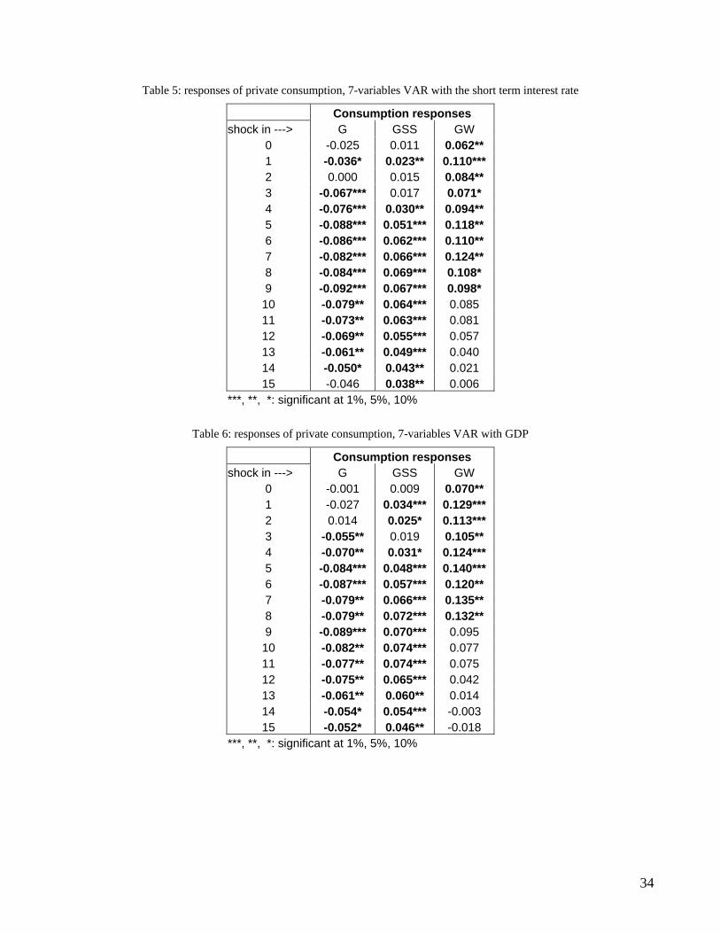
Table 5: responses of private consumption, 7-variables VAR with the short term interest rate

Consumption responses shock in ---> G GSS GW

0 -0.025 0.011 0.062** 1 -0.036* 0.023** 0.110*** 2 0.000 0.015 0.084** 3 -0.067*** 0.017 0.071* 4 -0.076*** 0.030** 0.094** 5 -0.088*** 0.051*** 0.118** 6 -0.086*** 0.062*** 0.110** 7 -0.082*** 0.066*** 0.124** 8 -0.084*** 0.069*** 0.108* 9 -0.092*** 0.067*** 0.098* 10 -0.079** 0.064*** 0.085 11 -0.073** 0.063*** 0.081 12 -0.069** 0.055*** 0.057 13 -0.061** 0.049*** 0.040 14 -0.050* 0.043** 0.021 15 -0.046 0.038** 0.006

***, **, *: significant at 1%, 5%, 10%

Table 6: responses of private consumption, 7-variables VAR with GDP

Consumption responses shock in ---> G GSS GW

0 -0.001 0.009 0.070** 1 -0.027 0.034*** 0.129*** 2 0.014 0.025* 0.113*** 3 -0.055** 0.019 0.105** 4 -0.070** 0.031* 0.124*** 5 -0.084*** 0.048*** 0.140*** 6 -0.087*** 0.057*** 0.120** 7 -0.079** 0.066*** 0.135** 8 -0.079** 0.072*** 0.132** 9 -0.089*** 0.070*** 0.095 10 -0.082** 0.074*** 0.077 11 -0.077** 0.074*** 0.075 12 -0.075** 0.065*** 0.042 13 -0.061** 0.060** 0.014 14 -0.054* 0.054*** -0.003 15 -0.052* 0.046** -0.018

***, **, *: significant at 1%, 5%, 10%

34

Table 7: responses of private consumption, 6-variables VAR (no financial liabilities)

Consumption responses shock in ---> G GSS GW

0 -0.014 0.010 0.060 1 -0.034 0.025** 0.109*** 2 0.000 0.015 0.094** 3 -0.072*** 0.010 0.082* 4 -0.088*** 0.021 0.103** 5 -0.097*** 0.033** 0.132*** 6 -0.097*** 0.042** 0.121** 7 -0.089*** 0.048*** 0.131** 8 -0.090*** 0.051*** 0.125** 9 -0.093*** 0.052*** 0.104* 10 -0.081*** 0.056*** 0.083 11 -0.072** 0.058*** 0.074 12 -0.068** 0.053*** 0.048 13 -0.059** 0.050*** 0.021 14 -0.049 0.046*** -0.002 15 -0.042 0.041** -0.020

***, **, *: significant at 1%, 5%, 10%

Table 8: responses of private consumption, 6-variables VAR (no net taxes)

Consumption responses shock in ---> G GSS GW

0 -0.018 0.010 0.022 1 -0.041** 0.025** 0.066* 2 0.006 0.013 0.039 3 -0.071*** 0.008 0.019 4 -0.079*** 0.017 0.046 5 -0.077*** 0.031** 0.073 6 -0.077*** 0.043*** 0.054 7 -0.074*** 0.048*** 0.075 8 -0.072** 0.052*** 0.082 9 -0.082** 0.051*** 0.064 10 -0.070** 0.049*** 0.049 11 -0.060** 0.045** 0.059 12 -0.060* 0.036** 0.055 13 -0.055 0.030* 0.045 14 -0.046 0.028* 0.042 15 -0.045 0.023 0.042

***, **, *: significant at 1%, 5%, 10%

35

Table 9: responses of private consumption, 6-variables VAR (no price index)

Consumption responses shock in ---> G GSS GW

0 -0.001 0.003 0.050 1 -0.019 0.016 0.103*** 2 0.024 0.001 0.071 3 -0.047 -0.006 0.067 4 -0.047 0.004 0.116** 5 -0.043 0.014 0.158*** 6 -0.041 0.021 0.136** 7 -0.036 0.026 0.145** 8 -0.037 0.029 0.144** 9 -0.050 0.030 0.122* 10 -0.039 0.033* 0.088 11 -0.031 0.033* 0.078 12 -0.031 0.027* 0.056 13 -0.028 0.028* 0.031 14 -0.026 0.028* 0.006 15 -0.027 0.027* -0.005

***, **, *: significant at 1%, 5%, 10%

Table 10: responses of private consumption, 5-variables VAR (with the three components of government expenditure)

Consumption responses shock in ---> G GSS GW

0 -0.016 0.013 0.219** 1 -0.029 0.027** 0.426*** 2 0.007 0.019 0.419*** 3 -0.061** 0.015 0.406*** 4 -0.073*** 0.022 0.490*** 5 -0.079*** 0.030** 0.569*** 6 -0.079** 0.036** 0.494*** 7 -0.073** 0.039** 0.527*** 8 -0.071** 0.042*** 0.518*** 9 -0.075** 0.044*** 0.459** 10 -0.063** 0.047*** 0.392* 11 -0.056* 0.050*** 0.369* 12 -0.055* 0.046*** 0.292 13 -0.049* 0.043*** 0.210 14 -0.041 0.042*** 0.141 15 -0.037 0.039*** 0.080

***, **, *: significant at 1%, 5%, 10%

36

Table 11: responses of private consumption, four 5-variables VARs with one government expenditure variable at a time

(note: differently from the previous tables, these are the results of 4 different VARs)

Consumption responses shock in ---> GTOT G GSS GW

0 0.006 -0.022 0.007 0.011 1 0.003 -0.048** 0.013 0.020 2 0.000 -0.022 0.006 -0.014 3 -0.023 -0.074*** 0.001 -0.044 4 -0.017 -0.086*** 0.014 -0.022 5 -0.011 -0.089*** 0.031 -0.020 6 -0.009 -0.087*** 0.039* -0.037 7 -0.004 -0.092*** 0.048** -0.046 8 -0.003 -0.095*** 0.052** -0.043 9 -0.003 -0.097*** 0.053** -0.052 10 -0.002 -0.088** 0.054** -0.059 11 -0.002 -0.082** 0.052** -0.060 12 -0.002 -0.079** 0.050** -0.059 13 -0.002 -0.072** 0.045** -0.061 14 -0.001 -0.064** 0.040** -0.057 15 0.001 -0.056* 0.036** -0.052

***, **, *: significant at 1%, 5%, 10%

37