Does government spending crowd in private consumption? Theory

WORKING PAPER SER IESNO. 513 / AUGUST 2005

DOES GOVERNMENTSPENDING CROWD IN

THEORY AND EMPIRICALEVIDENCE FOR THE EURO AREA

by Günter Coenenand Roland Straub

PRIVATE CONSUMPTION?

In 2005 all ECB publications will feature

a motif taken from the

€50 banknote.

WORK ING PAPER S ER I E SNO. 513 / AUGUST 2005

This paper can be downloaded without charge from http://www.ecb.int or from the Social Science Research Network

electronic library at http://ssrn.com/abstract_id=775424.

DOES GOVERNMENTSPENDING CROWD IN

PRIVATE CONSUMPTION?

THEORY AND EMPIRICALEVIDENCE FOR THE

EURO AREA 1

by Günter Coenen 2

and Roland Straub 3

1 This paper was prepared for the conference on “New Policy Thinking in Macroeconomics”, organised by the Maurice R. GreenbergCenter for Geoeconomic Studies, Council on Foreign Relations, with the support of McKinsey & Company and International Finance,

12 November, 2004. Earlier versions were circulated under the title “Non-Ricardian Households and Fiscal Policy in an Estimated DSGE Model of the Euro Area”. Useful comments and suggestions from Gregory de Walque, Ricardo Mestre, Paolo Pesenti,

Frank Smets, Javier Vallés, Jean-Pierre Vidal, Raf Wouters; our discussant, Margarida Duarte; an anonymous referee;and the editors, Fabio Ghironi and Benn Steil, are gratefully acknowledged.The opinions expressed are those of the

authors and do not necessarily reflect views of the European Central Bank or the International Monetary Fund.Any remaining errors are the sole responsibility of the authors.

2 Directorate General Research, European Central Bank; Postfach 16 03 19, D-60066 Frankfurt am Main, Germany;e-mail: [email protected], homepage: http://www.guentercoenen.com

3 Monetary and Financial Systems Department, International Monetary Fund; e-mail: [email protected]

© European Central Bank, 2005

AddressKaiserstrasse 2960311 Frankfurt am Main, Germany

Postal addressPostfach 16 03 1960066 Frankfurt am Main, Germany

Telephone+49 69 1344 0

Internethttp://www.ecb.int

Fax+49 69 1344 6000

Telex411 144 ecb d

All rights reserved.

Reproduction for educational and non-commercial purposes is permitted providedthat the source is acknowledged.

The views expressed in this paper do notnecessarily reflect those of the EuropeanCentral Bank.

The statement of purpose for the ECBWorking Paper Series is available fromthe ECB website, http://www.ecb.int.

ISSN 1561-0810 (print)ISSN 1725-2806 (online)

3ECB

Working Paper Series No. 513August 2005

CONTENTS

Abstract 4

Non-technical summary 5

1 Introduction 7

2 The model 11

2.1 Households 11

2.1.1 Ricardian households 12

2.1.2 Non-Ricardian households 14

2.1.3 Wage setting 14

2.1.4 Aggregation 16

2.2 Firms 17

2.2.1 Final-good firms 17

2.2.2 Intermediate-goods firms 18

2.2.3 Price setting 18

2.3 Fiscal and monetary authorities 19

2.4 Market clearing 20

3 Bayesian estimation of the model 21

3.1 Methodology 21

3.2 Data and prior distributions 22

3.3 Estimation results 24

4 Assessing the role of non-Ricardianhouseholds 28

4.1 Impulse-response analysis 29

4.2 Forecast-error-variance decomposition 33

5 Sensitivity analysis 37

6 Conclusions 40

References 42

European Central Bank working paper series 47

Abstract

In this paper, we revisit the effects of government spending shocks on private con-sumption within an estimated New-Keynesian DSGE model of the euro area featuringnon-Ricardian households. Employing Bayesian inference methods, we show that thepresence of non-Ricardian households is in general conducive to raising the level of con-sumption in response to government spending shocks when compared with the bench-mark specification without non-Ricardian households. However, we find that there isonly a fairly small chance that government spending shocks crowd in consumption,mainly because the estimated share of non-Ricardian households is relatively low, butalso due to the large negative wealth effect induced by the highly persistent nature ofgovernment spending shocks.

JEL Classification System: E32, E62

Keywords: non-Ricardian households, fiscal policy, DSGE modelling, euro area

4ECBWorking Paper Series No. 513August 2005

Non-Technical Summary

Micro-founded models of optimising agents are essential for evaluating the consequences

of alternative macroeconomic policies. As to the analysis of fiscal policy, it has long been

recognised that the introduction of non-Ricardian elements in these models play a crucial

role in obtaining meaningful results. Thus, a large body of literature has been oriented

towards gauging the implications of different forms of heterogeneity across households that

permit to evade Ricardian equivalence.

Recent research on the transmission of fiscal policy in New-Keynesian dynamic general

equilibrium (DSGE) models has introduced heterogeneity across households by assuming

that some households follow a simple rule of thumb and simply consume their after-tax

disposable income in each period (see, e.g., Galı, Lopez-Salido and Valles, 2004). As a

result of such non-Ricardian behaviour, transfer policies have real effects and the possibility

arises that a rise in government spending may crowd in private consumption, as suggested

by the empirical literature (see, e.g., Perotti, 2002; Fatas and Mihov, 2001; Canzoneri,

Cumby and Diba, 2002; and Mountford and Uhlig, 2001).

In this paper, we revisit the effects of government spending shocks on consumption util-

ising an extended version of the estimated euro area model by Smets and Wouters (2003).

This model supplements the standard New-Keynesian DSGE model with sticky prices by

adding sticky wages and various types of real frictions in an attempt to capture the high

degree of persistence characterising macroeconomic time series. In our extended version

of this model we allow, like Galı et al. (2004), for the co-existence of non-Ricardian and

Ricardian households. In addition, we allow for a more detailed fiscal policy framework

with a fiscal policy rule in place that stabilises the evolution of government debt and with

different types of distortionary taxes as well as lump-sum transfers. Adopting the empir-

ical approach used by Smets and Wouters, we first employ Bayesian estimation methods

to determine the relative importance of non-Ricardian households in the euro area under

different assumptions regarding the fiscal policy framework. We then proceed to analyse the

influences of non-Ricardian households and fiscal policy on the equilibrium dynamics of the

estimated model. In particular, we investigate the role played by non-Ricardian households

in the propagation of government spending and monetary policy shocks and in accounting

for observed fluctuations in consumption.

5ECB


Our results indicate that the estimated share of non-Ricardian households in the euro

area is relatively small, suggesting that financial deregulation over the last two decades

has lowered financial-market participation costs and lending support to the observation

that the effects of fiscal policy have become weaker over time (see, e.g., Fatas and Mihov,

2001; and Perotti, 2002). At the same time, we find that the inclusion of non-Ricardian

households in our model has important consequences for the estimation of the preference

parameters influencing the intertemporal consumption choices of Ricardian households. In

particular, the Ricardian households’ willingness to smooth consumption is found to be

lower than in the benchmark specification without non-Ricardian households. This, at least

partially, offsets the positive impact that non-Ricardian households exert on consumption

in response to government spending shocks. Nevertheless, we show that, when compared

with the benchmark specification, the inclusion of non-Ricardian households is in general

conducive to raising the level of consumption in response to a government spending shock,

notably in an environment where the tax burden largely rests with Ricardian households.

As a practical matter, however, we find that there is only a fairly small chance that a

government spending shock crowds in consumption, mainly because the estimated share

of non-Ricardian agents is relatively low, but also due to the large negative wealth effect

induced by the highly persistent nature of government spending shocks.


1 Introduction

Recent years have witnessed the development of a new generation of New-Keynesian

dynamic stochastic general equilibrium (DSGE) models that build on explicit microfoun-

dations with optimising agents. Major advances in estimation methodology allowed esti-

mating variants of these models that are able to compete with more standard time-series

models, such as vector autoregressions. Accordingly, the new generation of microfounded

DSGE models provides a framework that appears particularly suited for evaluating the

consequences of alternative macroeconomic policies.

While the literature has largely focused on using variants of the New-Keynesian DSGE

model to analyse the consequences of monetary policy, we are interested in elucidating

the effects of fiscal policy within such framework. Specifically, we focus on the effects of

government spending shocks on private consumption—an issue which has been at centre

stage of the policy debate for quite a long time. Standard versions of the New-Keynesian

DSGE model typically predict a strong negative response of consumption to government

spending shocks, while the empirical literature suggests that such shocks have a positive or,

at least, no significant negative effect on consumption (see, e.g., Perotti, 2002; Fatas and

Mihov, 2001; Canzoneri, Cumby and Diba, 2002; Mountford and Uhlig, 2001; and Galı,

Lopez-Salido and Valles, 2004). Clearly, in order to provide reliable policy advice, it is of

key importance to ascertain to which extent models used for quantitative policy analysis

can be reconciled with this established feature of the data.

The main reason for the failure of standard DSGE models to predict a positive consump-

tion response to government spending shocks has already been identified in a much simpler

Real Business Cycle (RBC) framework by Baxter and King (1993). As the authors show,

government spending shocks (financed by lump-sum taxes) generate a negative wealth effect

which induces households to work more but to consume less. Following the earlier analysis

by Baxter and King, there have been several attempts in the recent literature to resolve

the apparent consumption puzzle. Linnemann and Schabert (2003), for example, analyse

the effects of government spending shocks in a standard New-Keynesian sticky-price model.

The idea of introducing imperfect competition together with sticky prices into the RBC

7ECB


framework was promising for at least two reasons. First, imperfect competition generates

an aggregate demand externality according to which an increase in output leads to a rise

in profits and income. Higher profits and income in turn may help to offset the negative

wealth effect. Second, sticky prices raise the possibility that labour demand reacts stronger

than labour supply, with real wages increasing alongside labour supply. However, as shown

by Linnemann and Schabert, in the standard New-Keynesian model a positive consumption

response can only arise if monetary policy is sufficiently accommodative. Even a modestly

aggressive monetary policy rule implies a sharp decline in consumption after a government

spending shock because the households’ consumption choice is still dominated by the neg-

ative wealth effect. Thus, any successful attempt to resolve the consumption puzzle must

aim at dampening the dominant role of the latter.

In the standard New-Keynesian model, the negative wealth effect is amplified by the

fact that all households are forward looking and able to smooth consumption by trading in

physical and/or financial assets. As a consequence, consumption is a function of permanent

rather than current disposable income and “Ricardian equivalence” holds. However, there

is growing scepticism whether such framework represents a good approximation to reality.

Empirically, consumption seems to track current income more closely than predicted by

standard representative-agent models (see, e.g., Hall, 1978; and Campbell and Mankiw,

1989). In the light of this observation, Mankiw (2000) has emphasised the need to build a

new type of model for analysing the effects of fiscal policy shocks. Such type of model should

allow for heterogeneity of a particular form: some households should act in an optimising,

fully forward-looking manner, while others ought to follow a simple rule of thumb that

renders consumption smoothing impossible. Mankiw argues that such form of heterogeneity

can be easily reconciled with stylised facts at both the micro and macro level. First, by

reviewing micro studies on the consumption pattern of households in the United States,

Mankiw provides evidence supporting the view that consumption tracks current income

far more than it should. Evidently, there are many reasons why consumption smoothing

is far from perfect, amongst which the existence of borrowing and/or liquidity constraints,

myopia on the part of households and very high discounting are obvious candidates. Second,

based on the shape of the wealth and income distributions in the United States, Mankiw


concludes that a large fraction of households does not save and therefore does not have the

means to smooth consumption.

On the basis of this evidence, Galı, Lopez-Salido and Valles (2004) have extended

the standard New-Keynesian sticky-price model by allowing for the co-existence of

“non-Ricardian” and “Ricardian” households, with the former following a rule-of-thumb

and simply consuming their after-tax disposable income each period and the latter optimis-

ing in a forward-looking manner and thereby smoothing consumption over time. Galı et al.

demonstrate how the interaction of the two types of households with firms that infrequently

adjust prices and a fiscal authority which issues debt to finance part of its expenditure can

account for the existing evidence on the effects of government spending shocks. Notwith-

standing, the quantitative impact of a government spending shock on consumption largely

depends on the degree of debt financing and on whether the real wage increases or decreases

on impact. As a consequence, the response pattern of consumption is highly dependent on

the form of the fiscal policy rule and on how the real wage is determined in the labour mar-

ket. Regarding the latter, Galı et al. assume the existence of a generalised wage schedule

according to which households are willing to meet firms’ demand for labour at the real wage

offered. This assumption allows generating a sharp increase in the real wage after a gov-

ernment spending shock which in turn helps to offset the negative wealth effect. However,

as argued in Bilbiie and Straub (2004a), such sharp increase is at odds with the observed

a-cyclical behaviour of the real wage. Indeed, since standard RBC models predict strongly

pro-cyclical movements in the real wage, shocks to government spending have naturally

been thought of as an additional source of fluctuations that could help reduce the predicted

strong pro-cyclical pattern (see, e.g., Christiano and Eichenbaum, 1992). Moreover, the

real-wage response to government spending shocks tends to be small empirically (see, e.g.,

Fatas and Mihov, 2001).

In the light of this discussion, we revisit the effects of government spending shocks

on consumption utilising an extended version of the estimated euro area model by Smets

and Wouters (2003). This model supplements the standard New-Keynesian DSGE model

with sticky prices by adding sticky wages and various types of real frictions in an attempt

to capture the high degree of persistence characterising macroeconomic time series. In

9ECB


our extended version of this model we allow, like Galı et al., for the co-existence of non-

Ricardian and Ricardian households. In addition, we allow for a more detailed fiscal policy

framework with a fiscal policy rule in place that stabilises the evolution of government

debt and with different types of distortionary taxes as well as lump-sum taxes/transfers.

Adopting the empirical approach used by Smets and Wouters, we first employ Bayesian

estimation methods to determine the relative importance of non-Ricardian households in

the euro area under different assumptions regarding the fiscal policy framework. We then

proceed to analyse the influences of non-Ricardian households and fiscal policy on the

equilibrium dynamics of the estimated model. In particular, we investigate the role played

by non-Ricardian households in the propagation of government spending and monetary

policy shocks and in accounting for observed fluctuations in consumption.

Our results indicate that the estimated share of non-Ricardian households in the euro

area is relatively small, suggesting that financial deregulation over the last two decades

has lowered financial-market participation costs and lending support to the observation

that the effects of fiscal policy have become weaker over time (see, e.g., Fatas and Mihov,

2001; and Perotti, 2002). At the same time, we find that the inclusion of non-Ricardian

households in our model has important consequences for the estimation of the preference

parameters influencing the intertemporal consumption choices of Ricardian households. In

particular, the Ricardian households’ willingness to smooth consumption is found to be

lower than in the benchmark specification without non-Ricardian households. This, at least

partially, offsets the positive impact that non-Ricardian households exert on consumption

in response to government spending shocks. Nevertheless, we show that, when compared

with the benchmark specification, the inclusion of non-Ricardian households is in general

conducive to raising the level of consumption in response to a government spending shock,

notably in an environment where the tax burden largely rests with Ricardian households.

As a practical matter, however, we find that there is only a fairly small chance that a

government spending shock crowds in consumption, mainly because the estimated share

of non-Ricardian agents is relatively low, but also due to the large negative wealth effect

induced by the highly persistent nature of government spending shocks. In contrast to

the calibrated model used by Galı et al., we observe that our estimated model does not


generate a sharp increase in the real wage that would help to offset the negative wealth

effect. Finally, we document that reasonable variations in the parameters of the estimated

model have no qualitative impact on our findings.

The remainder of this paper is organised as follows. Section 2 outlines our extended

version of the Smets-Wouters (2003) model featuring non-Ricardian households. Section 3

briefly describes our empirical approach to estimating the extended model and documents

the estimation results. Section 4 investigates the importance of non-Ricardian households

for shaping the propagation of government spending and monetary policy shocks and for

explaining fluctuations in consumption. Section 5 reports the results of additional sensitivity

analysis, and Section 6 concludes.

2 The Model

Our model is an extended version of the medium-scale New-Keynesian DSGE model of the

euro area developed by Smets and Wouters (2003), henceforth referred to as SW (2003).

This model features four types of economic agents: households, firms, a monetary authority

and a fiscal authority, the latter being completely passive though. In our extended version,

we allow for two different types of households: optimising households, who can trade in

asset markets and thus are able to smooth consumption, and liquidity constrained house-

holds, who cannot participate in asset markets and therefore just consume their after-tax

disposable income. We also allow for a richer fiscal policy framework with a fiscal policy

rule stabilising the fiscal authority’s intertemporal budget and with distortionary taxes as

well as lump-sum taxes/transfers. In the following we briefly outline the behaviours of the

different types of agents.

2.1 Households

There is a continuum of households indexed by h ∈ [ 0, 1 ]. A share 1−ω of this continuum

of households—referred to as Ricardian households and indexed by i ∈ [ 0, 1 − ω )—have

access to financial markets, where they buy and sell government bonds, and accumulate

physical capital, the services of which they rent out to firms. The remaining share ω of

households—referred to as non-Ricardian households and indexed by j ∈ [ 1−ω, 1 ]—do not

11ECB


trade in assets and simply consume their after-tax disposable income.1 It is assumed that

the households supply differentiated labour services to a continuum of unions within the

household sector—indexed over the same range as the households, h ∈ [ 0, 1 ]—which act as

wage setters in monopolistically competitive markets. The unions pool the wage income of

all households and then distribute the aggregate wage income in equal proportions amongst

the latter. Formally, this may be justified by the existence of state-contingent securities that

are traded amongst unions in order to insure households against variations in household-

specific wage income. The households, in turn, are assumed to supply sufficient labour

services to satisfy labour demand.

2.1.1 Ricardian Households

Each Ricardian household i maximises its lifetime utility by choosing consumption, Ci,t,

investment, Ii,t, next period’s financial wealth in form of one-period government bonds,

Bi,t+1, next period’s physical capital stock, Ki,t+1, and the intensity with which the installed

capital stock is utilised, Zi,t, given the following lifetime utility function:

Et

[ ∞∑k=0

βkεbt+k

(1

1 − ς

(Ci,t+k − ϑ C∗

i,t+k−1

)1−ς − εnt+k

1 + ζ(Ni,t+k)

1+ζ) ]

. (1)

Here, β is the discount factor, ς denotes the coefficient of relative risk aversion and ζ is

the inverse of the elasticity of work effort with respect to the real wage. The parameter ϑ

measures the degree of external habit formation in consumption. Thus, the household’s

utility depends positively on the difference between the current, individually chosen level

of consumption, Ci,t, and the average consumption level that was chosen in the previous

period by the Ricardian peer group, C∗i,t−1, and negatively on labour supply, Ni,t.2 Two

serially correlated shocks enter the utility function: εbt = ρb εb

t−1 + ηbt is a preference shock

that affects the Ricardian household’s willingness to smooth consumption over time, and

εnt = ρn εn

t−1 + ηnt represents a shock to labour supply.

1While the notion of non-Ricardian behaviour typically refers to the misperception on the part of agentsthat a reduction in current taxes financed by a rise in government debt (i.e., by higher future tax liabilities)represents an increase in wealth, we follow the convention in the literature and label those households thatdo not trade in assets and simply consume their disposable income as non-Ricardian. Alternatively, Erceg,Guerrieri and Gust (2003) refer to hand-to-mouth households in this context.

2The pooling of wage income ensures that the marginal utility of wealth out of wage income is identicalacross Ricardian households. As a result, Ci,t = C∗

i,t holds in equilibrium.


The Ricardian household faces the following budget constraint (expressed in real terms):

(1 + τ c)Ci,t + Ii,t + R−1t

Bi,t+1

Pt+ Ψ(Zi,t)Ki,t (2)

=(1 − τd)(1 + τw)

Wt

PtNt + (1 − τd)

RKt

PtZi,t Ki,t + τd δ Ki,t + (1 − τd)

Di,t

Pt+

Ti,t

Pt+

Bi,t

Pt,

where the terms on the left-hand side show how the household uses its resources, while the

terms on the right-hand side indicate the resources the household has at its disposal. Rt

denotes the risk-less return on government bonds, and Pt is the aggregate price level. The

function Ψ( · ) represents the cost of varying the intensity of capital utilisation. RKt indicates

the rental rate for the capital services rent out to firms, Zi,t Ki,t, and Di,t are the dividends

paid by household-owned firms. The fiscal authority absorbs part of the gross income of

the household to finance government expenditure. τw is the pay-roll tax rate levied on the

household’s pooled wage income, Wt Nt, while τd denotes the income tax rate levied on all

sources of income (except for the returns on government bonds and minus physical capital

depreciation), and τ c is the consumption tax rate.3 Ti,t indicates lump-sum taxes paid (or

transfers received).

The capital stock owned by the Ricardian household evolves according to the following

capital accumulation equation,

Ki,t+1 = (1 − δ)Ki,t − (1 − Υ(εitIi,t/Ii,t−1)) Ii,t, (3)

where δ is the time-invariant depreciation rate, Υ( · ) represents a generalised adjustment

cost function in investment, and εit = ρi ε

it−1 + ηi

t is a serially correlated shock affecting

investment adjustment cost.

Letting Λt and Λt Qt denote the Lagrange multipliers associated with the budget con-

straint (2) and the capital accumulation equation (3), respectively, the first-order conditions

for maximising the household’s lifetime utility function (1) with respect to Ci,t, Ii,t, Bi,t+1,

Ki,t+1 and Zi,t are given—in that order—by:

(1 + τ c) Λt = εbt (Ci,t − ϑ C∗

i,t−1)−ς , (4)

3For simplicity, we assume that pay-roll taxes are paid by households alone. Similarly, it is assumed thatdividends are taxed at the household level.

13ECB


Qt

(1 − Υ(εi

tIi,t/Ii,t−1))

= Qt Υ′(εitIi,t/Ii,t−1) εi

t

Ii,t

Ii,t−1(5)

−β Et

[Λt+1

ΛtQt+1 Υ′(εi

t+1Ii,t+1/Ii,t) εit+1

I2i,t+1

I2i,t

]+ 1,

β Rt Et

[Λt+1

Λt

Pt

Pt+1

]= 1, (6)

Qt = β Et

[Λt+1

Λt

((1 − δ)Qt+1 + (1 − τd)

RKt+1

Pt+1Zi,t+1 + τd δ − Ψ(Zi,t+1)

)]+ ηq

t , (7)

(1 − τd)RK

t

Pt= Ψ′(Zi,t), (8)

where the latter condition implies that the intensity of capital utilisation is identical across

households; that is, Zi,t = Zt.

Following SW (2003), we have augmented equation (7), which determines the value of

installed capital (that is, Tobin’s Q), with a serially uncorrelated shock ηqt . This shock is

meant to capture stochastic variation in the external finance premium.4

2.1.2 Non-Ricardian Households

In our framework, the non-Ricardian households do not optimise—neither intertemporally

nor intratemporally. Each Ricardian household j simply follows a rule of thumb and sets

nominal consumption expenditure equal to after-tax disposable wage income:

(1 + τ c)Cj,t =(1 − τd)(1 + τw)

Wt

PtNt − Tj,t

Pt. (9)

Like for the Ricardian households, it is assumed that the non-Ricardian households take

the pooled wage income as given and supply sufficient labour services to satisfy labour

demand.

2.1.3 Wage Setting

There is a continuum of monopolistically competitive unions within the household sector

indexed by h ∈ [ 0, 1 ], which act as wage setters for the differentiated labour services4While this way of capturing stochastic variation in the external finance premium is largely ad hoc, it

could be justified on deeper grounds by introducing stochastic financial intermediation costs which wouldaffect the rental rate of capital. Here, as in SW, the inclusion of the shock is motivated by empiricalconsiderations.


supplied by the two types of households taking the aggregate nominal wage rate, Wt, and

aggregate labour demand, Nt, as given.

Following Calvo (1983), unions receive permission to optimally reset their nominal wage

rate in a given period t with probability 1 − ξw. All unions that receive permission to

reset their wage rate choose the same wage rate W ∗h,t. Those unions that do not receive

permission are allowed to adjust their wage rate at least partially according to the following

scheme:

Wh,t =(

Pt−1

Pt−2

)γw

Wh,t−1, (10)

where the parameter γw measures the degree of indexation to past changes in the aggregate

price index Pt.

Each union h that receives permission to optimally reset its wage rate in period t is

assumed to maximise household lifetime utility, as represented by equation (1), taking into

account the wage-indexation scheme (10) and the demand for labour services of variety h,

the latter being given by

Nh,t =(

Wh,t

Wt

)− 1+λw,tλw,t

Nt, (11)

where the stochastic parameter λw,t = λw+ηwt determines the wage markup in the unionised

labour markets.5

Hence, we obtain the following first-order condition for the union’s optimal wage-setting

decision in period t:6

Et

[ ∞∑k=0

ξkw βk Nh,t+k

(Λt+k

(1 − τd)(1 + τw)

W ∗h,t

Pt+k

(Pt+k−1

Pt−1

)γw

(12)

− (1 + λw,t+k) εnt+k (Nh,t+k)ζ

) ]= 0.

Aggregate labour demand, Nt, and the aggregate nominal wage rate, Wt, are determined5In the log-linear version of the model, the serially uncorrelated wage markup shock ηw

t can be interpretedas a cost-push shock to wage inflation.

6Alternatively, we could distinguish two groups of unions that act in the interest of either Ricardian ornon-Ricardian households. In this case, the unions would choose different wage rates, reflecting the differentconsumption patterns of the two types of households. As a practical matter, however, the differences in wagerates ought to be limited because our estimation results suggest that both the degree of wage stickiness, ξw,and the degree of indexation, γw, are relatively high.

15ECB


by the following Dixit-Stiglitz indices:

Nt =(∫ 1

0(Nh,t)

11+λw,t dh

)1+λw,t

, (13)

Wt =(∫ 1

0(Wh,t)

− 1λw,t dh

)−λw,t

. (14)

With the union-specific wage rates Wh,t set according to equation (10) and equation (12),

respectively, the evolution of the aggregate nominal wage rate (14) is then determined by

the following expression:

Wt =(

(1 − ξw)(W ∗h,t)

− 1λw,t + ξw

(Pt−1

Pt−2

)γw

(Wh,t−1)− 1

λw,t

)−λw,t

. (15)

2.1.4 Aggregation

The aggregate level in per-capita terms of any household-specific variable Xh,t is given by

Xt =∫ 10 Xh,t dh = (1−ω)Xi,t+ω Xj,t, as households in each of the two groups are identical.

Hence, aggregate consumption is given by

Ct = (1 − ω)Ci,t + ω Cj,t, (16)

while aggregate hours worked are given by

Nt = (1 − ω)Ni,t + ω Nj,t (17)

with the labour-market equilibrium being characterised by Nt = Ni,t = Nj,t.7

Since only Ricardian households hold financial assets, we obtain the following condition

for aggregate holdings of bonds:

Bt+1 = (1 − ω)Bi,t+1. (18)

Similarly, only Ricardian households accumulate physical capital,

Kt+1 = (1 − ω)Ki,t+1, (19)

It = (1 − ω) Ii,t, (20)

7This is a consequence of the assumption that unions pool the wage income of both groups of households.To ensure that pooling finally results in the same wage income, hours worked in both groups need to beequal in equilibrium.


and only Ricardian households receive dividends from firms,

Dt = (1 − ω)Di,t. (21)

Finally, aggregate lump-sum taxes/transfers are given by

Tt = (1 − ω)Ti,t + ω Tj,t. (22)

2.2 Firms

There are two types of firms. A continuum of monopolistically competitive firms indexed

by f ∈ [ 0, 1 ], each of which produces a single differentiated intermediate good, Yf,t, and a

distinct set of perfectly competitive firms, which combine all the intermediate goods into a

single final good, Yt.

2.2.1 Final-Good Firms

The final-good producing firms combine the differentiated intermediate goods Yf,t using a

standard Dixit-Stiglitz aggregator,

Yt =

(∫ 1

0Y

11+λp,t

f,t df

)1+λp,t

, (23)

where the stochastic parameter λp,t = λp + ηpt determines the price markup in the

intermediate-goods markets.8

Minimising the cost of production subject to the aggregation constraint (23) results in

demands for the differentiated intermediate goods as a function of their price Pf,t relative

to the price of the final good Pt,

Yf,t =(

Pf,t

Pt

)− 1+λp,tλp,t

Yt, (24)

where the price of the final good Pt is determined by the following index:

Pt =

(∫ 1

0P

− 1λp,t

f,t df

)−λp,t

. (25)

8In the log-linear version of the model, the serially uncorrelated price markup shock ηpt can be interpreted

as a cost-push shock to price inflation.

17ECB


2.2.2 Intermediate-Goods Firms

Each intermediate-goods firm f produces its differentiated output using an increasing-

returns-to-scale technology,

Yf,t = max[εat Kα

f,t N(1−α)f,t − Φ, 0

], (26)

utilising as inputs homogenous capital services rent from the households in a centralised

market, Kf,t = Zt Kf,t, and an index of differentiated labour services, Nf,t. The variable

εat = ρa εa

t−1 + ηat is a serially correlated technology shock, and the parameter Φ represents

fixed cost of production.9

Taking the rental cost of capital, RKt , and the aggregate wage index, Wt, as given, cost

minimisation subject to the production technology (26) yields first-order conditions for the

inputs which can be expressed as relative factor demands and nominal marginal cost:

Kf,t

Nf,t=

(α

1 − α

)Wt

RKt

, (27)

MCt =1

εat αα(1 − α)(1−α)

W(1−α)t (RK

t )α. (28)

2.2.3 Price Setting

Following Calvo (1983), intermediate-goods producing firms receive permission to optimally

reset their price in a given period t with probability 1−ξp. All firms that receive permission

to reset their price choose the same price P ∗f,t. Those firms which do not receive permission

are allowed to adjust their price at least partially according to the following scheme:

Pf,t =(

Pt−1

Pt−2

)γp

Pf,t−1, (29)

where the parameter γp measures the degree of indexation to past changes in the aggregate

price index Pt.

Each firm f receiving permission to optimally reset its price in period t maximises the

discounted sum of expected nominal profits,

Et

[ ∞∑k=0

ξkp χt,t+k Df,t+k

], (30)

9The fixed cost of production will be chosen to ensure zero profits in steady state. This in turn guaranteesthat there is no incentive for other firms to enter the market in the long run.


subject to the demand for its output (24) and the price-indexation scheme (29), where χt,t+k

is the stochastic discount factor of the households owning the firm and

Df,t = Pf,t Yf,t − MCt(Yf,t + Φ) (31)

are period-t nominal profits which are distributed as dividends to the households.

Hence, we obtain the following first-order condition for the firm’s optimal price-setting

decision in period t:

Et

[ ∞∑k=0

ξkp χt,t+k Yf,t+k

(P ∗

f,t

(Pt+k−1

Pt−1

)γp

− (1 + λp,t+k)MCt+k

)]= 0. (32)

With the intermediate-goods prices Pf,t set according to equation (29) and equation (32),

respectively, the evolution of the aggregate price index (25) is then determined by the

following expression:

Pt =(

(1 − ξp)(P ∗f,t)

− 1λp,t + ξp

(Pt−1

Pt−2

)γp

(Pf,t−1)− 1

λp,t

)−λp,t

. (33)

2.3 Fiscal and Monetary Authorities

The fiscal authority purchases the final good, Gt, issues bonds, Bt+1, and raises taxes

with details on the latter being given in Section 2.1 above. The fiscal authority’s budget

constraint then has the following form:

Gt +Bt

Pt=

τd

(1 + τw)Wt

PtNt + τd RK

t

PtZt Kt − τd δ Kt (34)

+ τd Dt

Pt+ τ c Ct +

Tt

Pt+ R−1

t

Bt+1

Pt,

where all quantities are expressed in real per-capita terms.

Since our model features non-Ricardian households, the time paths of government debt

and taxes matter for the evolution of the economy. To select amongst the set of feasible

time paths, and to stabilise government debt, we choose, as in Galı et al. (2004), a simple

log-linear fiscal policy rule:

tt = φb bt + φg gt, (35)

where φb and φg are the elasticities of lump-sum taxes with respect to government debt and

19ECB


government spending, respectively. Notice that tt, bt and gt are the log-linear counterparts

of lump-sum taxes, government debt and government spending, respectively.10

Here, government spending is assumed to evolve exogenously according to a serially

correlated process,

gt = ρg gt−1 + ηgt , (36)

where ηgt represents a serially uncorrelated shock.

As in SW (2003), the monetary authority sets the nominal interest rate according to a

simple log-linear monetary policy rule,

rt = φr rt−1 + (1 − φr) (πt + φπ (πt−1 − πt) + φy (yt − y∗t )) (37)

+ φ∆π (πt − πt−1) + φ∆y (yt − y∗t − (yt−1 − y∗t−1)) + ηrt ,

where rt = log(Rt/R) is the log-deviation of the nominal interest rate from its steady-

state value and πt = log(Pt/Pt−1) denotes the quarter-on-quarter inflation rate. yt is the

logarithm of aggregate output, while y∗t is the logarithm of the aggregate output level that

would prevail if wages and prices were flexible. πt = ρπ πt−1 + ηπt represents the monetary

authority’s inflation objective, which is assumed to follow a serially correlated process, with

mean zero and ηrt is a serially uncorrelated shock to the interest rate.

The particular form of the monetary policy rule—including a reaction to changes in both

inflation and the output gap—reflects empirical considerations. The time-varying inflation

objective is meant to capture the disinflation process in the run up to the formation of the

European Monetary Union in 1999.

2.4 Market Clearing

The labour market is in equilibrium when the demand for the index of labour services by the

intermediate-goods firms equals the differentiated labour services supplied by households

at the wage rates set by unions. Similarly, the market for physical capital is in equilibrium

when the demand for capital services by the intermediate-goods firms equals the capital10More specifically, we define the deviation of the fiscal variables from their respective steady-state values in

relative terms as a percentage of steady-state output; that is, tt = (Tt/Pt−T/P )/Y , bt = (Bt/Pt−1−B/P )/Yand gt = (Gt − G)/Y .


services supplied by households at the market rental rate. The market for government

bonds is in equilibrium when the outstanding government bonds are held by households at

the market interest rate. Lastly, the final-good market is in equilibrium when the supply

by the final-good firms equals the demand by households and government:

Yt = Ct + It + Gt + Ψ(Zt)Kt, (38)

where the last term accounts for the resource cost of varying the intensity of capital utili-

sation.

3 Bayesian Estimation of the Model

We adopt the empirical approach outlined in SW (2003) and estimate our augmented DSGE

model with non-Ricardian households employing Bayesian inference methods. This involves

obtaining the posterior distribution of the parameters of the model based on its log-linear

state-space representation and assessing its empirical performance in terms of its marginal

likelihood. In the following we briefly sketch the adopted approach and describe the data

and the prior distributions used in its implementation. We then present our estimation

results.

3.1 Methodology

Employing Bayesian inference methods allows formalising the use of prior information ob-

tained from earlier studies at both the micro and macro level in estimating the parameters

of a possibly complex DSGE model.11 This seems particularly appealing in situations where

the sample period of the data is relatively short, as is the case for the euro area. From a

practical perspective, Bayesian inference may also help to alleviate the inherent numerical

difficulties associated with solving the highly non-linear estimation problem.

Formally, let p(θ|m) denote the prior distribution of the parameter vector θ ∈ Θ for some

model m ∈ M, and let L(YT |θ, m) denote the likelihood function for the observed data,

YT = { yt }Tt=1, conditional on parameter vector θ and model m. The posterior distribution

11For recent examples of Bayesian estimation of DSGE models see Adolfson, Laseen, Linde and Villani(2004), Juillard, Karam, Laxton and Pesenti (2005), and Schorfheide and Lubik (2005).

21ECB


of the parameter vector θ for model m is then obtained by combining the likelihood function

for YT and the prior distribution of θ,

p(θ|YT , m) ∝ L(YT |θ, m) p(θ|m),

where “∝” indicates proportionality.

This distribution is typically characterised by standard measures of central location,

such as the mode or the mean, measures of dispersion, such as the standard deviation, or

selected percentiles.12

As discussed in Geweke (1999), Bayesian inference also provides a framework for compar-

ing non-nested and potentially misspecified models on the basis of their marginal likelihood.

For a given model m the latter is obtained by integrating out its parameter vector θ,

L(YT |m) =∫

θ∈ΘL(YT |θ, m) p(θ|m) dθ.

Thus, the marginal likelihood gives an indication of the overall likelihood of a model con-

ditional on the observed data.

3.2 Data and Prior Distributions

Since we wish to use the SW model as our benchmark for assessing the performance of

the augmented DSGE model with non-Ricardian households, we follow SW (2003) in our

implementation of the Bayesian estimation methodology as closely as possible. Thus, as

in SW, we estimate the augmented model using aggregate euro area data on real GDP,

consumption, investment, employment, wage income, GDP inflation and the short-term

nominal interest rate. The data cover the period 1980Q1 through 1999Q4. Real variables

are expressed in logarithms and then detrended by removing individual linear trends, while

inflation and the interest rate are detrended under the assumption that these variables share

a common linear trend reflecting the protracted disinflation process prior to the formation of12As in SW (2003), and following Schorfheide (2000), we adopt a Monte-Carlo Markov-Chain (MCMC)

sampling method to determine the posterior distribution of the parameter vector θ. More specifically, we relyon the Metropolis-Hastings (MH) algorithm to obtain a large number of random draws from the posteriordistribution of θ. The mode and the Hessian of the posterior distribution, the latter evaluated at the mode,are used to initialise the MH algorithm. For all computations, we employ the Dynare software of Juillard(2004).


the European Monetary Union in 1999.13 We also allow for ten exogenous shocks driving the

stochastic behaviour of the model: four serially correlated shocks arising from preferences

and technology (εbt , εn

t , εat and εi

t), three serially uncorrelated cost-push shocks affecting price

and wage setting and the price of installed capital (ηpt , ηw

t and ηqt ), a serially correlated

government spending shock (gt), and two monetary policy shocks (ηrt and πt) capturing

unexpected moves in the short-term nominal interest rate and persistent changes in the

monetary authority’s unobserved inflation objective, respectively. Although we will focus

on the consequences of only a subset of these shocks in the subsequent analysis, the inclusion

of a comprehensive set of shocks is important in order to match the time-series properties

of the data satisfactorily.

Regarding the choice of prior distributions for the parameters of the model, we follow

SW (2003) in fixing several parameters throughout the estimation. This includes setting

the subjective discount factor β to 0.99, the production function parameter α to 0.3, the

depreciation rate δ to 0.025 and the steady-state wage markup λw to 0.5. The steady-state

ratios of government spending and government debt over GDP, G/Y and (B/P )/Y , are set

equal to 0.18 and 0.6× 4, respectively. Most of these parameters are related to the steady-

state values of observed variables in an obvious way. In contrast to SW, we assume that the

steady-state price markup λp is equal to the share of the fixed costs in production, Φ/Y ,

implying zero profits in steady state. For versions of the model incorporating distortionary

taxation, we set the income tax rate τd, the pay-roll tax rate τw and the consumption tax

rate τ c equal to 0.14, 0.45 and 0.20, respectively.14

We also follow SW (2003) in choosing the same prior distributions for the parameters

that need to be estimated and that are common to the benchmark model and our aug-

mented specification. A complete listing of the details on the prior distributions, including

their means and standard deviations, can be found in Appendix Table A. Here, we only

wish to mention that the preference, technology, and price and wage-setting parameters13As in SW, we use the period 1970Q1 to 1979Q4 to obtain good initial values of the unobserved variables

in the model’s linear state-space representation and then use the period 1980Q1 to 1999Q4 to compute thelikelihood with the Kalman filter.

14The calibration of tax rates is based on the time series of government revenues contained in the dataset provided by Fagan, Henry and Mestre (2001). Lacking a more detailed break down of tax categories, weuse indirect taxes minus subsidies as our proxy for consumption taxes. The results documented below arerobust to reasonable variations in the steady-state tax rates.

23ECB


are assumed to follow either a Normal distribution or a Beta distribution, the latter con-

straining individual parameters to fall in the range of zero to one, if prescribed by theory.

The parameters controlling the persistence of the shock processes are assumed to have a

Beta distribution with uniform mean 0.85 and uniform standard deviation 0.1. The latter

assumption facilitates the identification of persistent as opposed to non-persistent shocks.

The conditional standard deviations of the shock processes are assumed to have an Inverted

Gamma distribution with two degrees of freedom. This distribution guarantees a positive

standard deviation with a relatively large support. Finally, the parameters of the monetary

policy rule are assumed to follow a Normal distribution, except for the coefficient on the

lagged nominal interest rate which is assumed to follow a Beta distribution.

The prior distributions which remain to be specified are those for the share of non-

Ricardian households, ω, and the parameters of the fiscal policy rule, φb and φg. In line with

the baseline calibrations used in Galı et al. (2004), we assume that ω has a Beta distribution

with mean 0.5 and standard deviation 0.1. This value is consistent with estimates obtained

by Campbell and Mankiw (1989) for the fraction of liquidity-constrained households in the

United States for the pre-1990 period. The fiscal policy parameter prescribing the response

of lump-sum taxes to debt, φb, is assumed to follow an Inverted Gamma distribution with

mean 0.1 and degrees of freedom equal to 2.15 Finally, the parameter governing the response

of lump-sum taxes to government spending is assumed to have a Normal distribution with

mean 0.1 and standard deviation 0.05.

3.3 Estimation Results

Table 1 reports the means of the posterior distributions for a subset of parameters that

are a priori considered to be of particular relevance in accounting for possible differences

between the benchmark specification of SW (2003) and our augmented specification with

non-Ricardian households.16 In total, we report estimation results for four different speci-

fications, including the benchmark specification of SW and three alternative specifications15The choice of the Inverted Gamma distribution guarantees that the likelihood of obtaining estimates

that result in unstable debt dynamics is negligible.16Further estimation results are reported in Appendix Table B. The 10% and 90% percentiles of the

posterior distributions are available from the authors on request.


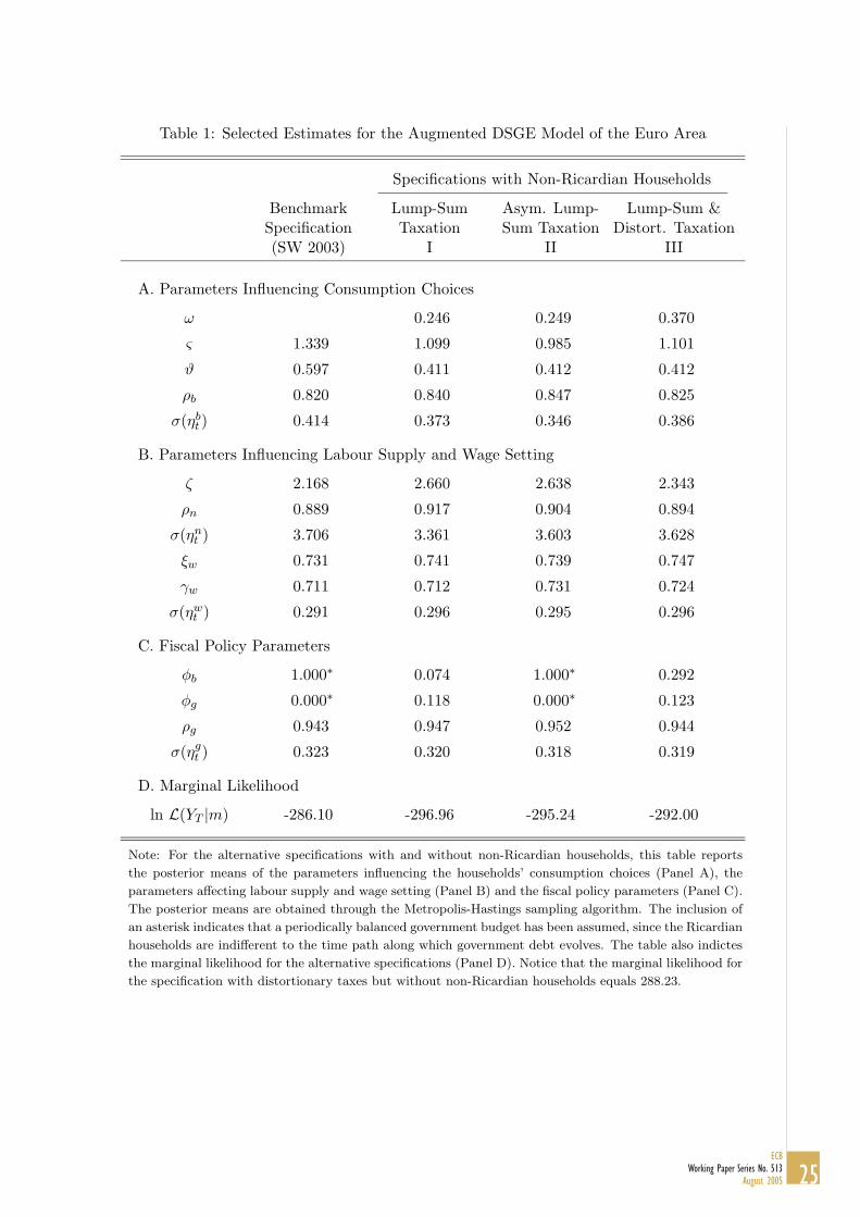
Table 1: Selected Estimates for the Augmented DSGE Model of the Euro Area

Specifications with Non-Ricardian Households

Benchmark Lump-Sum Asym. Lump- Lump-Sum &Specification Taxation Sum Taxation Distort. Taxation(SW 2003) I II III

A. Parameters Influencing Consumption Choices

ω 0.246 0.249 0.370

ς 1.339 1.099 0.985 1.101

ϑ 0.597 0.411 0.412 0.412

ρb 0.820 0.840 0.847 0.825

σ(ηbt ) 0.414 0.373 0.346 0.386

B. Parameters Influencing Labour Supply and Wage Setting

ζ 2.168 2.660 2.638 2.343

ρn 0.889 0.917 0.904 0.894

σ(ηnt ) 3.706 3.361 3.603 3.628

ξw 0.731 0.741 0.739 0.747

γw 0.711 0.712 0.731 0.724

σ(ηwt ) 0.291 0.296 0.295 0.296

C. Fiscal Policy Parameters

φb 1.000∗ 0.074 1.000∗ 0.292

φg 0.000∗ 0.118 0.000∗ 0.123

ρg 0.943 0.947 0.952 0.944

σ(ηgt ) 0.323 0.320 0.318 0.319

D. Marginal Likelihood

ln L(YT |m) -286.10 -296.96 -295.24 -292.00

Note: For the alternative specifications with and without non-Ricardian households, this table reports

the posterior means of the parameters influencing the households’ consumption choices (Panel A), the

parameters affecting labour supply and wage setting (Panel B) and the fiscal policy parameters (Panel C).

The posterior means are obtained through the Metropolis-Hastings sampling algorithm. The inclusion of

an asterisk indicates that a periodically balanced government budget has been assumed, since the Ricardian

households are indifferent to the time path along which government debt evolves. The table also indictes

the marginal likelihood for the alternative specifications (Panel D). Notice that the marginal likelihood for

the specification with distortionary taxes but without non-Ricardian households equals 288.23.

25ECB


with non-Ricardian households that differ with respect to the details of the tax scheme

in place.17 In the first two out of these three alternative specifications, we only consider

lump-sum taxation; that is, we set the distortionary tax rates equal to zero. Specification I

assumes that both Ricardian and non-Ricardian households pay lump-sum taxes in equal

proportions, while specification II assumes that the levied lump-sum taxes are unevenly

distributed across the two groups of households. Specifically, we consider the extreme case

where non-Ricardian households are completely exempted from paying taxes to exemplify

the differences in household behaviour. Specification III extends specification I by also in-

corporating distortionary taxes: an income tax levied on all sources of income (except for

returns on bonds), a pay-roll tax on wage income and a tax on consumption. To the extent

that these specifications affect the income at the disposal of non-Ricardian households in

different ways, they are a priori expected to have quite different implications for the role of

non-Ricardian households in the propagation of shocks.

Panel A of Table 1 indicates the posterior means of the parameters directly influencing

the consumption choices of Ricardian and non-Ricardian households, including the share

of non-Ricardian households, ω, the preference parameters ς and ϑ, and the parameters

governing the process of the intertemporal preference shock, ρb and σ(ηbt ). Here, σ( · )

generically indicates the (conditional) standard deviation of a shock. Starting with the pos-

terior mean of ω, we observe that the estimated share of non-Ricardian households is quite

a bit smaller than the mean of the prior distribution which was set equal 0.5 on the basis

of estimates obtained for the pre-1990 period in the United States (see, e.g., Campbell and

Mankiw, 1989). Specifically, the posterior mean of the share of non-Ricardian households

equals one-fourth or roughly one-third, depending on the presence of distortionary taxes.

A possible interpretation of this finding is that our sample only covers observations from

the period 1980 through 1999 which was a period of far-reaching financial deregulation that

dramatically reduced financial-market participation costs.18

17Small deviations of the estimates reported for the benchmark specification from those reported in SWmay result from using a slightly extended sample, incorporating capital utilisation cost in the aggregateresource constraint, small discrepancies in the calibration of the model’s steady state as well as differencesin the implementation of the Metropolis-Hastings sampling algorithm.

18This interpretation is consistent with the findings of Bilbiie and Straub (2004b) who show that the shareof non-Ricardian households in the United States fell significantly after the Depository and Institutions


At the same time, the inclusion of non-Ricardian households has some noticeable effects

on the parameters influencing the intertemporal consumption choices of Ricardian house-

holds. In particular, the estimated intertemporal elasticity of substitution, 1/ς, is quite

a bit larger than the estimate obtained for the benchmark specification, implying a lower

willingness to smooth consumption on the part of Ricardian households. In fact, for the

specifications featuring non-Ricardian households the estimated intertemporal elasticity of

substitution is close to unity and consumption preferences are thus broadly consistent with

a logarithmic specification. Similarly, the estimated degree of habit formation ϑ is signifi-

cantly smaller than the estimate obtained for the benchmark specification. Consequently,

changes in the short-term interest rate ought to have a comparatively large impact on the

consumption choices of Ricardian households.

Panel B of Table 1 reports the posterior means of the parameters affecting labour supply

and unionised wage setting. The estimate of the inverse elasticity of labour supply with

respect to the real wage, ζ, turns out to be somewhat higher in the specifications with

non-Ricardian households. However, variations in the labour-supply elasticity of this order

of magnitude have little consequence for the dynamics of the type of model examined

in this paper. Similarly, we observe some variation in the estimates of the parameters

characterising the labour-supply shock, ρn and σ(ηnt ), although these estimates tend to

move in opposite directions, leaving the unconditional variation of the labour-supply shocks

across specifications broadly unchanged. Finally, the posterior means of the parameters

influencing the unions’ wage-setting decisions, ξw, γw and σ(ηwt ), are virtually unaffected

by the inclusion of non-Ricardian households.

Panel C shows the posterior means of the fiscal policy parameters. Of course, in the

benchmark specification without non-Ricardian households, but also in the specification

where non-Ricardian households are assumed to be exempted from paying taxes, the par-

ticular time path along which government debt evolves does not matter and, thus, we have

imposed a periodically balanced government budget with φb = 1 and φg = 0. For the two

remaining specifications, we observe quite some heterogeneity regarding the responsiveness

of lump-sum taxes to government debt, φb, with the posterior mean being equal to 0.07

Deregulation and Monetary Control Act (DIDMCA) had passed legislation in 1980.

27ECB


or 0.29, depending on the presence of distortionary taxes. In contrast, the fraction of gov-

ernment spending that is instantaneously financed by lump-sum taxes, φg, has a mean of

about 0.12, irrespective of the presence of distortionary taxes. Not surprisingly, the param-

eters of the exogenous shock process characterising government spending, ρg and σ(ηgt ), are

very similar across all four specifications. Importantly, the estimated degree of persistence

is close to 0.95 and, hence, government spending shocks ought to induce a large negative

wealth effect in the model.

Finally, Panel D indicates the marginal likelihood for the four specifications which al-

lows to assess their relative performance conditional on the data. Surprisingly, none of

the augmented specifications with non-Ricardian households succeeds in outperforming the

benchmark model. Obviously, there may be various reasons for this relatively poor em-

pirical performance of the augmented model. For example, the presence of non-Ricardian

households, while tilting the operating characteristics of the model in response to govern-

ment spending shocks in the desired direction, may adversely affect the response pattern

of the model to alternative shocks, possibly originating in the influence that the inclusion

of non-Ricardian households exerts on the estimated preference parameters. Alternatively,

the quantitative importance of government spending shocks may possibly be overstated

when evaluated through the lens of a New-Keynesian model allowing for non-Ricardian

elements. In the subsequent analysis we will therefore systematically examine the role of

non-Ricardian households for the equilibrium dynamics of the model.

4 Assessing the Role of Non-Ricardian Households

Having estimated alternative specifications of the augmented DSGE model of the euro

area, we now proceed to investigate the role played by non-Ricardian households in the

propagation of shocks and in accounting for observed fluctuations in consumption to enhance

our understanding of the relatively poor empirical performance of the specifications with

non-Ricardian households. In this context, we focus our analysis on the effects of government

spending and monetary policy shocks, but also review the consequences of a number of

other shocks that have been identified in the previous section as potentially important for

explaining the influences of non-Ricardian households on consumption dynamics.


4.1 Impulse-Response Analysis

For each of the four estimated specifications, Figure 1 depicts the dynamic responses of

selected variables to a persistent government spending shock equal to one percent of steady-

state output. For ease of comparison, the parameter governing the degree of persistence is

set equal to the posterior mean of ρg = 0.943 that has been obtained for the benchmark

specification without non-Ricardian households. All dynamic responses are depicted as

percentage-point deviations from steady state.

As can be seen in the upper left panel in Figure 1, aggregate consumption in the bench-

mark specification without non-Ricardian households (referred to as benchmark and in-

dicated by a solid line) falls noticeably on impact in response to a government spending

shock before gradually returning to steady state, with the adjustment path exhibiting a

hump-shaped pattern. Apparently, for the augmented specifications I to III featuring non-

Ricardian households aggregate consumption falls by less when compared to the consump-

tion response in the benchmark specification. Yet again, in all three specifications with

non-Ricardian households government spending shocks fail to crowd in aggregate consump-

tion and thereby do not generate a fiscal multiplier with respect to output that exceeds one.

Even worse, the stronger impact effect of government spending shocks is very short-lived and

eventually followed by a lasting period of pronounced under-shooting of the consumption

path obtained in the benchmark specification.

Comparing the consumption patterns of Ricardian and non-Ricardian households helps

to understand the differences in the dynamic response pattern of aggregate consumption

across specifications. As shown in the middle right panel of Figure 1, the government

spending shock succeeds, at least on impact, in stimulating consumption on the part of

non-Ricardian households, regardless of the tax scheme in place. For the specification with

evenly distributed lump-sum taxes (specification I, dashed line), for example, consumption

increases on impact by about 0.5 percentage points. However, consumption starts falling

below its steady-state level already after a few quarters, because the build up of govern-

ment debt leads to a rise in lump-sum taxes which in turn lowers after-tax disposable income

29ECB


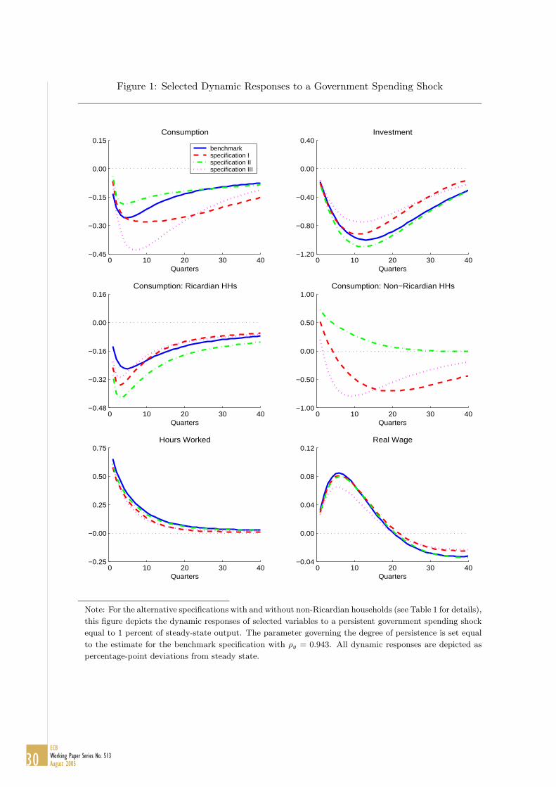
Figure 1: Selected Dynamic Responses to a Government Spending Shock

0 10 20 30 40−0.45

−0.30

−0.15

0.00

0.15Consumption

Quarters

benchmarkspecification Ispecification IIspecification III

0 10 20 30 40−1.20

−0.80

−0.40

0.00

0.40Investment

Quarters

0 10 20 30 40−0.48

−0.32

−0.16

0.00

0.16Consumption: Ricardian HHs

Quarters 0 10 20 30 40

−1.00

−0.50

0.00

0.50

1.00Consumption: Non−Ricardian HHs

Quarters

0 10 20 30 40−0.25

−0.00

0.25

0.50

0.75Hours Worked

Quarters 0 10 20 30 40

−0.04

0.00

0.04

0.08

0.12Real Wage

Quarters

Note: For the alternative specifications with and without non-Ricardian households (see Table 1 for details),

this figure depicts the dynamic responses of selected variables to a persistent government spending shock

equal to 1 percent of steady-state output. The parameter governing the degree of persistence is set equal

to the estimate for the benchmark specification with ρg = 0.943. All dynamic responses are depicted as

percentage-point deviations from steady state.


and thereby crowds out consumption. When non-Ricardian households are exempted from

paying lump-sum taxes (specification II, dashed-dotted line), we observe that the impact

multiplier is considerably larger and, importantly, that consumption never falls below its

steady-state level in the course of the adjustment process. By contrast, for the specifica-

tion which, in addition, incorporates distortionary taxes (specification III, dotted line) the

impact multiplier is cut in half when compared with the specification that features lump-

sum taxation alone. In this case, after-tax disposable income is reduced even more due to

the households’ income and pay-roll tax obligations. Above and beyond, consumption is

retrenched by the existence of the consumption tax.

As regards the consumption profile of Ricardian households, it can be seen in the middle

left panel of Figure 1 that consumption falls on impact even further than in the bench-

mark specification, with the return to steady state eventually somewhat faster though.

Thus, while an increase in government spending positively affects consumption spending

of non-Ricardian households, at least on impact, this effect tends to be offset by a fall in

consumption on the part of Ricardian households. Clearly, with the estimated share of

non-Ricardian households being relatively small, the overall effect of government spending

shocks on aggregate consumption turns out to be negative.

The lower two panels in Figure 1 depict the responses of hours worked and the real

wage. On impact, hours worked increase substantially, reflecting the surge in labour demand

following the government spending shock. In contrast, while moving in the desired direction,

the real wage rises by only very little due to the high degree of rigidity characterising wage-

setting decisions. This feature of our estimated model contrasts with the much simpler

calibrated set up in Galı et al. (2004). The latter abstracts from inertia in the wage-

setting process and incorporates a static labour demand schedule instead according to which

households are willing to meet firms’ demand for labour at the real wage offered. This

static set up implies, quite mechanistically, a sharp rise in the real wage in response to a

government spending shock, which in turn boosts disposable income and helps to crowd in

aggregate consumption, at least on impact.19

19For a critical discussion of the labour demand schedule proposed by Galı et al. (2004) and its importancefor generating a crowding-in effect see also Mihov (2003).

31ECB


Figure 2: The Response of Monetary Policy to a Government Spending Shock

0 10 20 30 40−0.06

0.00

0.06

0.12

0.18

0.24Nominal Interest Rate

Quarters


0 10 20 30 40−0.09

0.00

0.09

0.18

0.27

0.36Output Gap

Quarters

0 10 20 30 40−0.02

0.00

0.02

0.04

0.06

0.08Inflation Rate

Quarters 0 10 20 30 40

−0.03

0.00

0.03

0.06

0.09

0.12Real Marginal Cost

Quarters

Note: For the alternative specifications with and without non-Ricardian households, (see Table 1 for

details), this figure depicts the dynamic responses of selected variables to a persistent government spending

shock equal to 1 percent of steady-state output. The parameter governing the degree of persistence is set

equal to the estimate for the benchmark specification with ρg = 0.943. All dynamic responses are depicted

as percentage-point deviations from steady state.

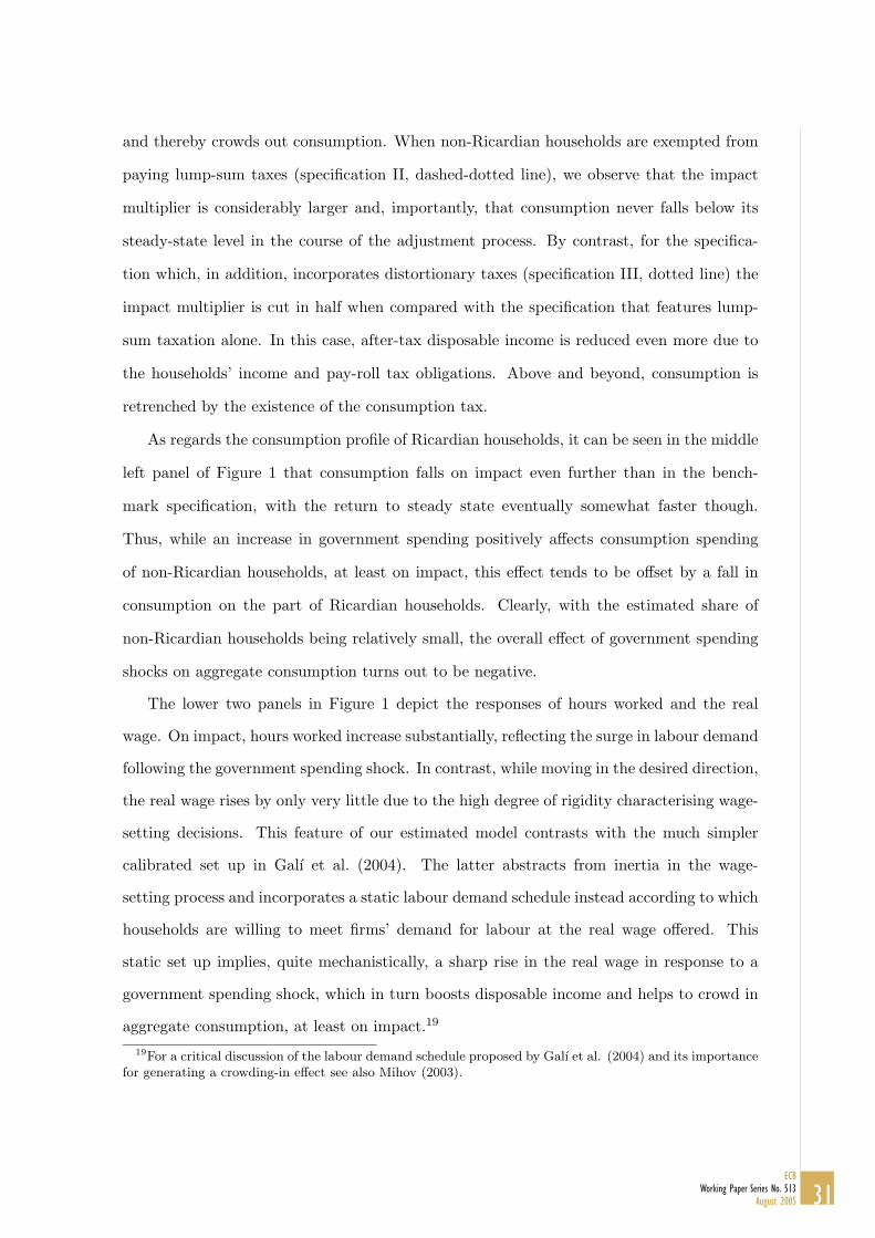
To cast further light on the consequences of a government spending shock in our esti-

mated model, Figure 2 portrays the dynamic responses of monetary policy, as captured by

the short-term nominal interest rate, together with the responses of those variables most

influential for the monetary authority’s rule-based interest-rate decision. As can be seen

in the upper right panel of the figure, in the specifications with non-Ricardian households

the size of the output gap building up in response to a government spending shock exceeds

that in the benchmark specification by almost one-tenth of a percentage point, with the


output gap being computed relative to the flexible-price and wage equilibrium. In contrast,

the lower left panel shows that the inflation effect is fairly small and roughly comparable

across specifications. As demonstrated in the lower right panel, this reflects that the time

profile of real marginal cost—the key driver of inflation—is largely similar. Ultimately, as

shown in the upper left panel, the more sizeable response of the output gap dominates and

thus results in a more pronounced tightening of monetary policy in the specifications with

non-Ricardian households. Consistent with the response pattern exposed in Figure 1 above,

this exacerbates the decline in consumption spending on the part of Ricardian households,

thereby further curbing the impact of a government spending shock.

Finally, Figure 3 depicts the consequences of a monetary policy shock corresponding

to an unexpected one-quarter increase in the short-term nominal interest rate equal to 25

basis points, with the monetary authority following the estimated policy rule thereafter. As

shown in the upper left panel of the figure, a rise in the short-term nominal interest rate

has a comparatively large negative impact on aggregate consumption in the specifications

with non-Ricardian households. As can be seen in the middle left panel, this echoes, at

least in the initial periods, a disproportionate fall in consumption on the part of Ricardian

households. As we emphasised in our discussion of the estimation results, the latter reflects

that the estimates of both the inverse of the intertemporal elasticity of substitution and the

degree of habit formation are quite a bit smaller in the specifications with non-Ricardian

households. As a consequence, the interest-rate elasticity of consumption is higher, yielding

a stronger decline in consumption after a monetary policy shock. However, regarding the

overall effect on output, we observe that the stronger decline in aggregate consumption is

at least partially offset by a more subdued fall in investment. We also observe that the

decrease in hours worked and the real wage is uniformly smaller.

4.2 Forecast-Error-Variance Decomposition

To provide additional insights into the various mechanisms through which non-Ricardian

households may influence the dynamic consumption responses in our model, we analyse

the contributions of selected shocks to the forecast-error variance of aggregate consump-

tion and its sub-components at various horizons. The results of the forecast-error-variance

33ECB


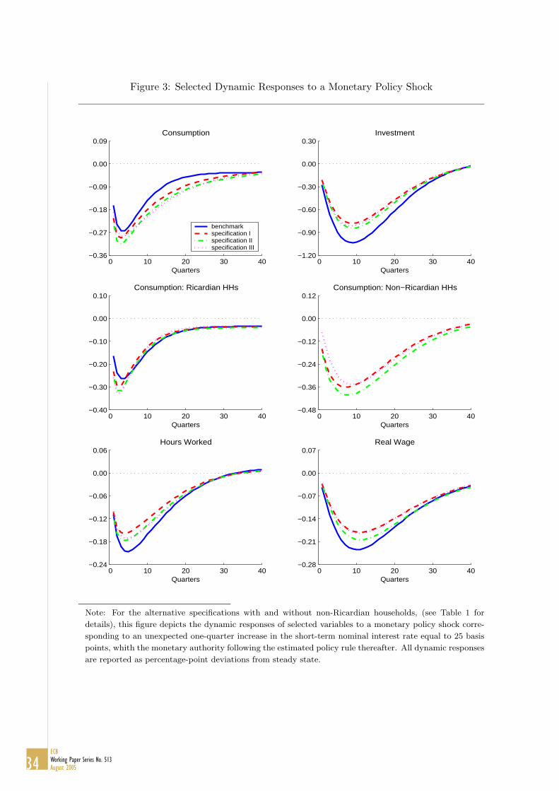
Figure 3: Selected Dynamic Responses to a Monetary Policy Shock

0 10 20 30 40−0.36

−0.27

−0.18

−0.09

0.00

0.09Consumption

Quarters


0 10 20 30 40−1.20

−0.90

−0.60

−0.30

0.00

0.30Investment

Quarters

0 10 20 30 40−0.40

−0.30

−0.20

−0.10

0.00

0.10Consumption: Ricardian HHs

Quarters 0 10 20 30 40

−0.48

−0.36

−0.24

−0.12

0.00

0.12Consumption: Non−Ricardian HHs

Quarters

0 10 20 30 40−0.24

−0.18

−0.12

−0.06

0.00

0.06Hours Worked

Quarters 0 10 20 30 40

−0.28

−0.21

−0.14

−0.07

0.00

0.07Real Wage

Quarters

Note: For the alternative specifications with and without non-Ricardian households, (see Table 1 for

details), this figure depicts the dynamic responses of selected variables to a monetary policy shock corre-

sponding to an unexpected one-quarter increase in the short-term nominal interest rate equal to 25 basis

points, whith the monetary authority following the estimated policy rule thereafter. All dynamic responses

are reported as percentage-point deviations from steady state.


decomposition are summarised in Table 2, contrasting the results for the benchmark spec-

ification with those for the augmented specification featuring non-Ricardian households

and uniformly distributed lump-sum taxes. We focus on those shocks that have already

been identified above as primarily important for discerning the influences of non-Ricardian

households, namely the government spending shock, the intertemporal preference shock,

the labour supply shock and the wage markup shock. In addition, we also report results for

the monetary policy shock.

By comparing the results for the benchmark specification in Panel A of Table 2 with

those for the specification with non-Ricardian households in Panel B, it can be seen that the

contributions of the selected shocks to the forecast-error variance of aggregate consumption

are broadly similar across the two specifications. Nevertheless, while differences in the

contributions of government spending shocks are hardly discernible at longer horizons, the

contributions of government spending shocks are found to be noticeably smaller at shorter

horizons in the specification with non-Ricardian households. This is consistent with a more

limited crowding-out effect on impact due to the presence of non-Ricardian households

(see Figure 1 above). Another noteworthy discrepancy is exhibited by the contributions

of wage markup shocks. The latter are found to have a positive, albeit small short-run

effect on aggregate consumption in the specification with non-Ricardian households, which

is virtually zero in the benchmark specification.

Contrasting the results obtained for the sub-components of aggregate consumption, as

shown in the lower part of Panel B in Table 2, reveals a number of notable differences that

are conducive to a better understanding of the aggregate results. First, in the short run,

government spending shocks account for about 3 percent of the fluctuations in consumption

of non-Ricardian households, while they account for only half a percent in the case of Ricar-

dian households. Second, since preference shocks do not directly influence the consumption

decision of non-Ricardian households, they explain, regardless of the forecast horizon, only

about 15 percent of the variation in non-Ricardian households’ consumption, compared to

roughly 60 percent for Ricardian households. Similarly, for non-Ricardian households the

contribution of labour supply shocks is significantly smaller than for Ricardian households.

On the contrary, wage markup shocks, which directly affect the after-tax disposable income

35ECB


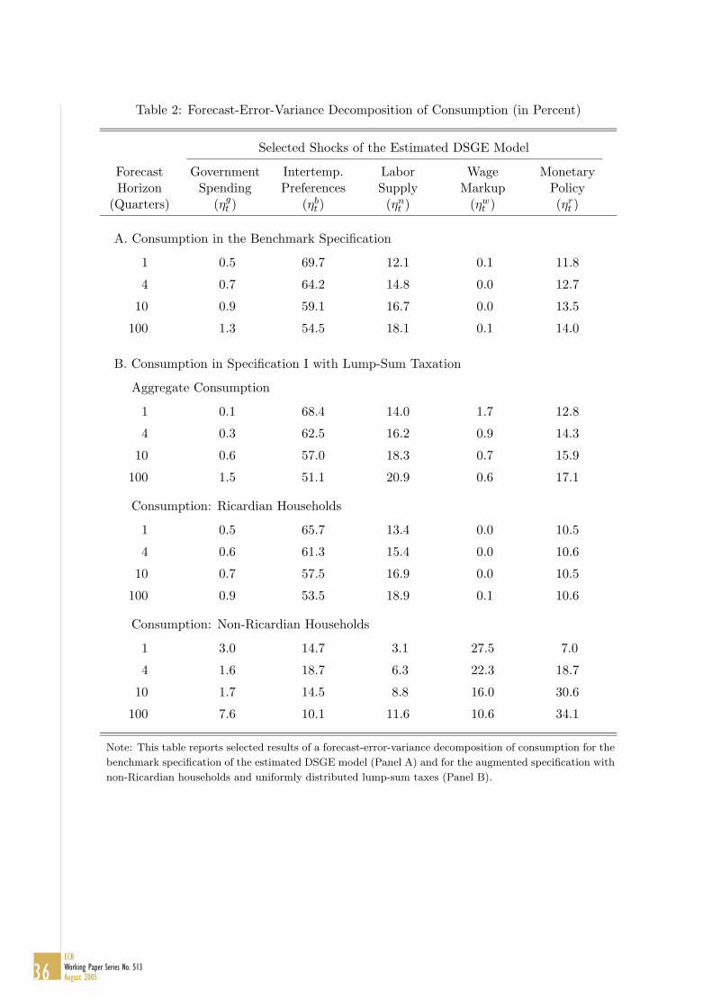
Table 2: Forecast-Error-Variance Decomposition of Consumption (in Percent)

Selected Shocks of the Estimated DSGE Model

Forecast Government Intertemp. Labor Wage MonetaryHorizon Spending Preferences Supply Markup Policy

(Quarters) (ηgt ) (ηb

t ) (ηnt ) (ηw

t ) (ηrt )

A. Consumption in the Benchmark Specification

1 0.5 69.7 12.1 0.1 11.8

4 0.7 64.2 14.8 0.0 12.7

10 0.9 59.1 16.7 0.0 13.5

100 1.3 54.5 18.1 0.1 14.0

B. Consumption in Specification I with Lump-Sum Taxation

Aggregate Consumption

1 0.1 68.4 14.0 1.7 12.8

4 0.3 62.5 16.2 0.9 14.3

10 0.6 57.0 18.3 0.7 15.9

100 1.5 51.1 20.9 0.6 17.1

Consumption: Ricardian Households

1 0.5 65.7 13.4 0.0 10.5

4 0.6 61.3 15.4 0.0 10.6

10 0.7 57.5 16.9 0.0 10.5

100 0.9 53.5 18.9 0.1 10.6

Consumption: Non-Ricardian Households

1 3.0 14.7 3.1 27.5 7.0

4 1.6 18.7 6.3 22.3 18.7

10 1.7 14.5 8.8 16.0 30.6

100 7.6 10.1 11.6 10.6 34.1

Note: This table reports selected results of a forecast-error-variance decomposition of consumption for the

benchmark specification of the estimated DSGE model (Panel A) and for the augmented specification with

non-Ricardian households and uniformly distributed lump-sum taxes (Panel B).


of non-Ricardian households, account for more than 25 percent of the short-run fluctua-

tions. All in all, the fact that the estimated share of non-Ricardian households amounts

to less than one-fourth may then explain why only fairly small effects can be observed at

the aggregate level. Furthermore, the effects of shocks that influence Ricardian and non-

Ricardian households in opposite ways, such as the government spending shock, may at

least partially cancel out each other.

5 Sensitivity Analysis

We finally present some additional sensitivity analysis to shed light on the general ability

of our estimated model to generate crowding-in effects with regard to consumption or even

an overall fiscal multiplier larger than one in response to a government spending shock. To

this end, we appraise the impact effect of a government spending shock on consumption

(aggregated and dis-aggregated) and investment that results when a single parameter is

varied holding all other parameters constant at their estimated values. Clearly, if the

parameters can vary over a relatively broad range of values without resulting in a large

increase in consumption on impact, there may be no realistic chance to generate an overall

fiscal multiplier that exceeds one within the framework of our estimated model.

Figure 4 depicts the sensitivity of the impact multiplier of a government spending

shock for the specification with non-Ricardian households and uniformly distributed lump-

sum taxes. We focus on those parameters that are most likely to have a positive influence

on the size of the consumption response, notably the share of non-Ricardian households, ω,

the fiscal policy parameters, ρg, φb and φg, and the parameters influencing unionised wage-

setting decisions, ξw and γw. Each panel of the figure shows the percentage-point deviation

from steady state for aggregate consumption, consumption on the part of both Ricardian

and non-Ricardian households and aggregate investment as a single parameter is varied,

with the estimated mean of the parameter indicated by a solid vertical line.

The upper left panel in Figure 4 depicts the sensitivity of the impact multiplier to vari-

ations in the share of non-Ricardian households, ω. Once the value of ω exceeds 0.35, the

response of aggregate consumption to a government spending shock turns out to be positive,

with the response of investment remaining broadly unchanged. In contrast, as shown in the

37ECB


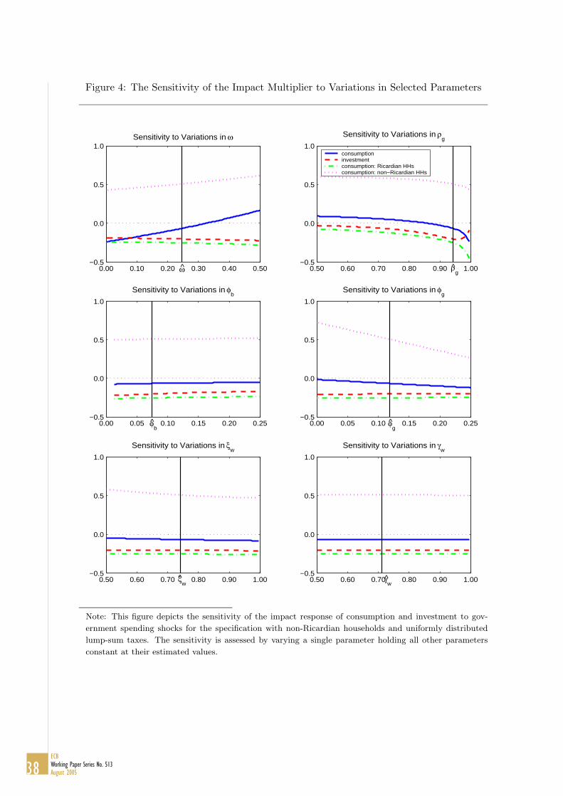
Figure 4: The Sensitivity of the Impact Multiplier to Variations in Selected Parameters

0.00 0.10 0.20 0.30 0.40 0.50−0.5

0.0

0.5

1.0Sensitivity to Variations in ω

ω 0.50 0.60 0.70 0.80 0.90 1.00−0.5

0.0

0.5

1.0

Sensitivity to Variations in ρg

ρg

consumptioninvestmentconsumption: Ricardian HHsconsumption: non−Ricardian HHs

0.00 0.05 0.10 0.15 0.20 0.25−0.5

0.0

0.5

1.0

Sensitivity to Variations in φb

φb

0.00 0.05 0.10 0.15 0.20 0.25−0.5

0.0

0.5

1.0

Sensitivity to Variations in φg

φg

0.50 0.60 0.70 0.80 0.90 1.00−0.5

0.0

0.5

1.0

Sensitivity to Variations in ξw

ξw

0.50 0.60 0.70 0.80 0.90 1.00−0.5

0.0

0.5

1.0

Sensitivity to Variations in γw

γw

Note: This figure depicts the sensitivity of the impact response of consumption and investment to gov-

ernment spending shocks for the specification with non-Ricardian households and uniformly distributed

lump-sum taxes. The sensitivity is assessed by varying a single parameter holding all other parameters

constant at their estimated values.


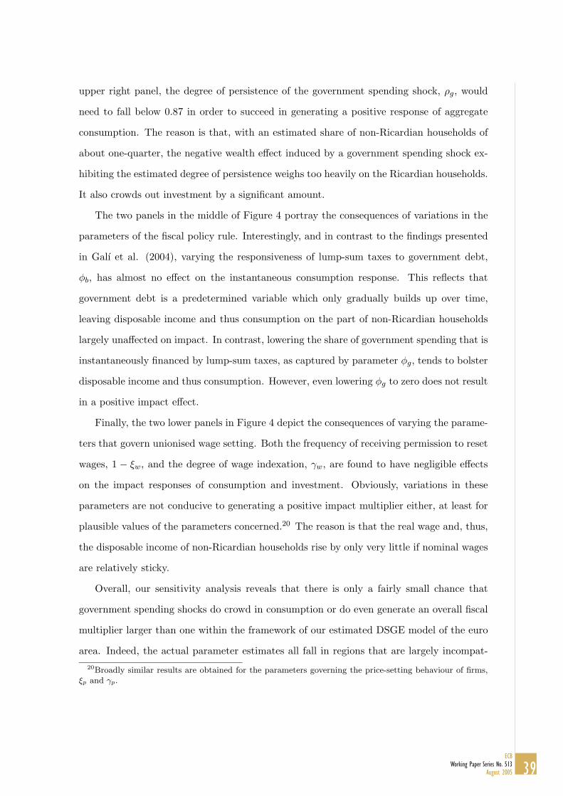
upper right panel, the degree of persistence of the government spending shock, ρg, would

need to fall below 0.87 in order to succeed in generating a positive response of aggregate

consumption. The reason is that, with an estimated share of non-Ricardian households of

about one-quarter, the negative wealth effect induced by a government spending shock ex-

hibiting the estimated degree of persistence weighs too heavily on the Ricardian households.

It also crowds out investment by a significant amount.

The two panels in the middle of Figure 4 portray the consequences of variations in the

parameters of the fiscal policy rule. Interestingly, and in contrast to the findings presented

in Galı et al. (2004), varying the responsiveness of lump-sum taxes to government debt,

φb, has almost no effect on the instantaneous consumption response. This reflects that

government debt is a predetermined variable which only gradually builds up over time,

leaving disposable income and thus consumption on the part of non-Ricardian households

largely unaffected on impact. In contrast, lowering the share of government spending that is

instantaneously financed by lump-sum taxes, as captured by parameter φg, tends to bolster

disposable income and thus consumption. However, even lowering φg to zero does not result

in a positive impact effect.

Finally, the two lower panels in Figure 4 depict the consequences of varying the parame-

ters that govern unionised wage setting. Both the frequency of receiving permission to reset

wages, 1 − ξw, and the degree of wage indexation, γw, are found to have negligible effects

on the impact responses of consumption and investment. Obviously, variations in these

parameters are not conducive to generating a positive impact multiplier either, at least for

plausible values of the parameters concerned.20 The reason is that the real wage and, thus,

the disposable income of non-Ricardian households rise by only very little if nominal wages

are relatively sticky.

Overall, our sensitivity analysis reveals that there is only a fairly small chance that

government spending shocks do crowd in consumption or do even generate an overall fiscal

multiplier larger than one within the framework of our estimated DSGE model of the euro

area. Indeed, the actual parameter estimates all fall in regions that are largely incompat-20Broadly similar results are obtained for the parameters governing the price-setting behaviour of firms,

ξp and γp.

39ECB


ible with a positive response of aggregate consumption to a government spending shock.

Notwithstanding these findings, the analysis suggests that the inclusion of non-Ricardian

households does tilt the consumption response to government spending shocks in the desired

direction. At the same time, the negative wealth effect induced by government shocks still

weighs too heavily on Ricardian households. This points to a need to modify the model in

directions which help to further mitigate the induced negative wealth effect.

6 Conclusions

In this paper, we have undertaken an attempt to reconcile the existing evidence on the

effects of government spending shocks with the predictions of a New-Keynesian DSGE

model that builds on explicit microfoundations with optimising agents. To account for the

limited ability of households to smooth consumption over time we have modified the model

by allowing for the co-existence of non-Ricardian and Ricardian households. Employing

Bayesian inference methods to estimate this model for the euro area over the period 1980

through 1999, we find that the estimated share of non-Ricardian households in the euro

area is relatively small, tentatively suggesting that financial deregulation over the last two

decades has lowered financial-market participation costs. At the same time, we show that

the presence of non-Ricardian households is in general conducive to raising the level of

consumption in response to government spending shocks when compared with a benchmark

specification of the model without non-Ricardian households. However, there is only a

fairly small chance that government spending shocks do actually crowd in consumption.

The main reason is that the estimated share of non-Ricardian households is relatively low.

In order to predict crowding-in effects, the model would need to be modified in directions

which help to further mitigate the negative wealth effect induced by the highly persistent

nature of government spending shocks.

While our model allows for a relatively detailed fiscal policy set up with different types

of taxes that determine government revenues and a fiscal policy rule that stabilises gov-

ernment debt, this paper has proceeded under the simplifying assumption that government

spending evolves exogenously according to a highly persistent shock process. In subsequent

work it will be interesting to explore the consequences when agents have limited information


about the future path of exogenous government spending shocks and must form expecta-

tions about the nature of unobserved shocks. As shown in Erceg, Guerrieri and Gust (2003),

such mechanism may help to reduce the negative wealth effect induced by highly persis-

tent government spending shocks. Similarly, the induced negative wealth effect is likely to

be mitigated once the possibility of an endogenous response of the long-run government

debt-to-GDP ratio to persistent government spending shocks is taken into account. These

extensions may ultimately lessen the need to include non-Ricardian elements; but, at the

same time, they may help to improve the empirical performance of the model. Finally, in

the light of empirical evidence that distortionary taxes tend to rise in response to lasting

increases in government spending (see, e.g., Fatas and Mihov, 2001; and Burnside, Eichen-

baum and Fisher, 2003), it would also be interesting to extend the analysis by allowing for

alternative fiscal policy rules with distortionary rather than lump-sum taxes responding to

developments in government spending and debt.

41ECB


References

Adolfson, M., S, Laseen, J. Linde and M. Villani, 2004, “Bayesian Estimation of an OpenEconomy DSGE Model with Incomplete Pass-Through”, Manuscript, Sveriges Riks-bank.

Baxter, M. and R. King, 1993, “Fiscal Policy in General Equilibrium”, American Eco-nomic Review, 83, 315-344.

Bilbiie, F. and R. Straub, 2004a, “Fiscal Policy, Business Cycles and Labor Market Fluc-tuations”, Magyar Nemzeti Bank Working Paper 2004/6.

Bilbiie, F. and R. Straub, 2004b, “Limited Asset Market Participation and Aggregate De-mand: A Rationale for US Monetary Policy during the Great Inflation”, Manuscript,European University Institute.

Burnside, C., M. Eichenbaum and J. D. M. Fisher, 2003, “Fiscal Shocks and Their Conse-quences”, Manuscript, Northwestern University.

Calvo, G. A., 1983, “Staggered Prices in a Utility-Maximizing Framework”, Journal ofMonetary Economics, 12, 383-398.

Campbell, J. Y., and N. G. Mankiw, 1989, “Consumption, Income, and Interest Rates:Reinterpreting the Time Series Evidence”, in O. J. Blanchard and S. Fischer (eds),NBER Macroeconomics Annual, Cambridge: MIT Press, 185-216.

Canzoneri, M. B., R. Cumby and B. Diba, 2002, “Should the European Central Bank andthe Federal Reserve Be Concerned about Fiscal Policy?”, in Rethinking StabilizationPolicy, Symposium sponsered by the Federal Reserve Bank of Kansas City, JacksonHole, Wyoming, 333-389.

Christiano, L. and M. Eichenbaum, 1992, “Current Real Business Cycle Theories and Ag-gregate Labor Market Fluctutations”, American Economic Review, 82, 430-450.

Erceg, C. J., L. Guerrieri and C. Gust, 2003, “SIGMA: A New Open Economy Model forPolicy Analyis”, Manuscript, Board of Governors of the Federal Reserve System.

Fagan, G., J. Henry, and R. Mestre, 2001, “An Area-Wide Model (AWM) for the EuroArea”, ECB Working Paper No. 42, European Central Bank, January.

Fatas, A. and I. Mihov, 2001, “The Effects of Fiscal Policy on Consumption and Employ-ment: Theory and Evidence”, Manuscript, INSEAD.

Galı, J., J. D. Lopez-Salido and J. Valles, 2004, “Understanding the Effects of GovernmentSpending on Consumption”, ECB Working Paper No. 339, European Central Bank,April.

Geweke, J. F., 1999, “Using Simulation Methods for Bayesian Econometric Models: Infer-ence, Developments and Communication” (with discussion and rejoinder), Economet-ric Reviews, 18, 1-126.

Hall, R. E., 1978, “Stochastic Implications of the Life Cycle-Permanent Income Hypothesis:Theory and Evidence”, Journal of Political Economy, 86, 971-987.


Juillard, M., 2004, “Dynare Manual”, Manuscript, CEPREMAP.

Juillard, M., P. Karam, D. Laxton and P. Pesenti, 2005, “Welfare-Based Monetary PolicyRules in an Estimated DSGE Model of the U.S. Economy”, Manuscript, InternationalMonetary Fund.

Linnemann, L. and A. Schabert, 2003, “Fiscal Policy in the New Neoclassical Synthesis”,Journal of Money, Credit and Banking, 35, 911-929.

Mankiw, N. G., 2000, “The Savers-Spenders Theory of Fiscal Policy”, American EconomicReview, 90, 120-125.

Mihov, I., 2003, Discussion of “Understanding the Effect of Government Spending on Con-sumption” by J., Galı, J. D. Lopez-Salido and J. Valles, International Research Forumon Monetary Policy, Washington, DC, November.

Mountford, A. and H. Uhlig, 2001, “What Are the Effects of Fiscal Policy Shocks?”, Cen-tER Discussion Paper No. 31, Tilburg University.

Perotti, R., 2002, “Estimating the Effects of Fiscal Policy in OECD Countries”, Manu-script, European University Institute.

Schorfheide, F., 2000, “Loss-Function-Based Evaluation of DSGE Models”, Journal of Ap-plied Econometrics, 15, 645-670.

Schorfheide, F. and T. Lubik, 2005, “A Bayesian Look at New Open Economy Macroeco-nomics”, Manuscript, University of Pennsylvania.

Smets, F. and R. Wouters, 2003, “An Estimated Stochastic Dynamic General EquilibriumModel of the Euro Area”, Journal of the European Economic Association, 1, 1123-1175.

43ECB


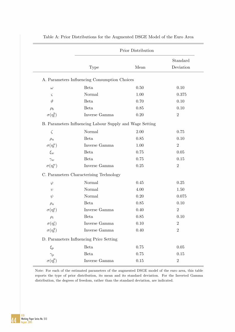
Table A: Prior Distributions for the Augmented DSGE Model of the Euro Area

Prior Distribution

Standard

Type Mean Deviation

A. Parameters Influencing Consumption Choices

ω Beta 0.50 0.10

ς Normal 1.00 0.375

ϑ Beta 0.70 0.10

ρb Beta 0.85 0.10

σ(ηbt ) Inverse Gamma 0.20 2

B. Parameters Influencing Labour Supply and Wage Setting

ζ Normal 2.00 0.75

ρn Beta 0.85 0.10

σ(ηnt ) Inverse Gamma 1.00 2

ξw Beta 0.75 0.05

γw Beta 0.75 0.15

σ(ηwt ) Inverse Gamma 0.25 2

C. Parameters Characterising Technology

ϕ Normal 0.45 0.25

υ Normal 4.00 1.50

ψ Normal 0.20 0.075

ρa Beta 0.85 0.10

σ(ηat ) Inverse Gamma 0.40 2

ρi Beta 0.85 0.10

σ(ηit) Inverse Gamma 0.10 2

σ(ηqt ) Inverse Gamma 0.40 2

D. Parameters Influencing Price Setting

ξp Beta 0.75 0.05

γp Beta 0.75 0.15

σ(ηpt ) Inverse Gamma 0.15 2

Note: For each of the estimated parameters of the augmented DSGE model of the euro area, this table

reports the type of prior distribution, its mean and its standard deviation. For the Inverted Gamma

distribution, the degrees of freedom, rather than the standard deviation, are indicated.


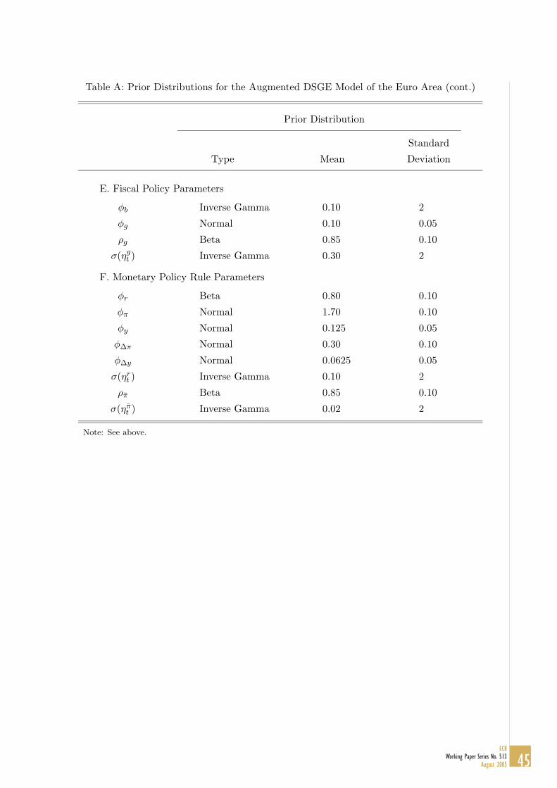
Table A: Prior Distributions for the Augmented DSGE Model of the Euro Area (cont.)

Prior Distribution

Standard

Type Mean Deviation

E. Fiscal Policy Parameters

φb Inverse Gamma 0.10 2

φg Normal 0.10 0.05

ρg Beta 0.85 0.10

σ(ηgt ) Inverse Gamma 0.30 2

F. Monetary Policy Rule Parameters

φr Beta 0.80 0.10

φπ Normal 1.70 0.10

φy Normal 0.125 0.05

φ∆π Normal 0.30 0.10

φ∆y Normal 0.0625 0.05

σ(ηrt ) Inverse Gamma 0.10 2

ρπ Beta 0.85 0.10

σ(ηπt ) Inverse Gamma 0.02 2

Note: See above.

45ECB


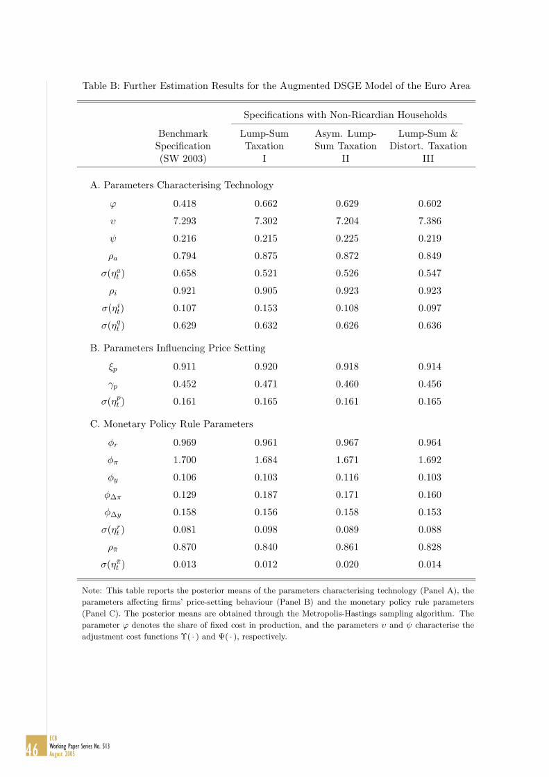
Table B: Further Estimation Results for the Augmented DSGE Model of the Euro Area

Specifications with Non-Ricardian Households

Benchmark Lump-Sum Asym. Lump- Lump-Sum &Specification Taxation Sum Taxation Distort. Taxation(SW 2003) I II III

A. Parameters Characterising Technology

ϕ 0.418 0.662 0.629 0.602

υ 7.293 7.302 7.204 7.386

ψ 0.216 0.215 0.225 0.219

ρa 0.794 0.875 0.872 0.849

σ(ηat ) 0.658 0.521 0.526 0.547

ρi 0.921 0.905 0.923 0.923

σ(ηit) 0.107 0.153 0.108 0.097

σ(ηqt ) 0.629 0.632 0.626 0.636

B. Parameters Influencing Price Setting

ξp 0.911 0.920 0.918 0.914

γp 0.452 0.471 0.460 0.456

σ(ηpt ) 0.161 0.165 0.161 0.165

C. Monetary Policy Rule Parameters

φr 0.969 0.961 0.967 0.964

φπ 1.700 1.684 1.671 1.692

φy 0.106 0.103 0.116 0.103

φ∆π 0.129 0.187 0.171 0.160

φ∆y 0.158 0.156 0.158 0.153

σ(ηrt ) 0.081 0.098 0.089 0.088

ρπ 0.870 0.840 0.861 0.828

σ(ηπt ) 0.013 0.012 0.020 0.014

Note: This table reports the posterior means of the parameters characterising technology (Panel A), the

parameters affecting firms’ price-setting behaviour (Panel B) and the monetary policy rule parameters

(Panel C). The posterior means are obtained through the Metropolis-Hastings sampling algorithm. The

parameter ϕ denotes the share of fixed cost in production, and the parameters υ and ψ characterise the

adjustment cost functions Υ( · ) and Ψ( · ), respectively.


47ECB


European Central Bank working paper series

For a complete list of Working Papers published by the ECB, please visit the ECB’s website(http://www.ecb.int)

482 “Forecasting macroeconomic variables for the new member states of the European Union”by A. Banerjee, M. Marcellino and I. Masten, May 2005.

483 “Money supply and the implementation of interest rate targets” by A. Schabert, May 2005.

484 “Fiscal federalism and public inputs provision: vertical externalities matter” by D. Martínez-López,May 2005.

485 “Corporate investment and cash flow sensitivity: what drives the relationship?” by P. Mizenand P. Vermeulen, May 2005.

486 “What drives productivity growth in the new EU member states? The case of Poland”by M. Kolasa, May 2005.

487 “Computing second-order-accurate solutions for rational expectation models using linearsolution methods” by G. Lombardo and A. Sutherland, May 2005.

488 “Communication and decision-making by central bank committees: different strategies,same effectiveness?” by M. Ehrmann and M. Fratzscher, May 2005.

489 “Persistence and nominal inertia in a generalized Taylor economy: how longer contracts dominateshorter contracts” by H. Dixon and E. Kara, May 2005.

490 “Unions, wage setting and monetary policy uncertainty” by H. P. Grüner, B. Hayo and C. Hefeker,June 2005.

491 “On the fit and forecasting performance of New-Keynesian models” by M. Del Negro,F. Schorfheide, F. Smets and R. Wouters, June 2005.

492 “Experimental evidence on the persistence of output and inflation” by K. Adam, June 2005.

493 “Optimal research in financial markets with heterogeneous private information: a rationalexpectations model” by K. Tinn, June 2005.

494 “Cross-country efficiency of secondary education provision: a semi-parametric analysis withnon-discretionary inputs” by A. Afonso and M. St. Aubyn, June 2005.

495 “Measuring inflation persistence: a structural time series approach” by M. Dossche andG. Everaert, June 2005.

496 “Estimates of the open economy New Keynesian Phillips curve for euro area countries”by F. Rumler, June 2005.

497 “Early-warning tools to forecast general government deficit in the euro area:the role of intra-annual fiscal indicators” by J. J. Pérez, June 2005.

498 “Financial integration and entrepreneurial activity: evidence from foreign bank entry in emergingmarkets” by M. Giannetti and S. Ongena, June 2005.

499 “A trend-cycle(-season) filter” by M. Mohr, July 2005.


500 “Fleshing out the monetary transmission mechanism: output composition and the role of financialfrictions” by A. Meier and G. J. Müller, July 2005.

501 “Measuring comovements by regression quantiles” by L. Cappiello, B. Gérard, and S. Manganelli, July 2005.

502 “Fiscal and monetary rules for a currency union” by A. Ferrero, July 2005

503 “World trade and global integration in production processes: a re-assessment of import demandequations” by R. Barrell and S. Dées, July 2005.

504 “Monetary policy predictability in the euro area: an international comparison”by B.-R. Wilhelmsen and A. Zaghini, July 2005.

505 “Public good issues in TARGET: natural monopoly, scale economies, network effects and cost allocation”by W. Bolt and D. Humphrey, July 2005.

506 “Settlement finality as a public good in large-value payment systems”by H. Pagès and D. Humphrey, July 2005.

507 “Incorporating a “public good factor” into the pricing of large-value payment systems”by C. Holthausen and J.-C. Rochet, July 2005.

508 “Systemic risk in alternative payment system designs” by P. Galos and K. Soramäki, July 2005.

509 “Productivity shocks, budget deficits and the current account” by M. Bussière, M. Fratzscherand G. J. Müller, August 2005.

510 “Factor analysis in a New-Keynesian model” by A. Beyer, R. E. A. Farmer, J. Henryand M. Marcellino, August 2005.

511 “Time or state dependent price setting rules? Evidence from Portuguese micro data”by D. A. Dias, C. R. Marques and J. M. C. Santos Silva, August 2005.

512 “Counterfeiting and inflation” by C. Monnet, August 2005.

513 “Does government spending crowd in private consumption? Theory and empirical evidence forthe euro area” by G. Coenen and R. Straub, August 2005.

Documents

Does government spending crowd in private consumption? Theory