The Residual:On Monitoring and Benchmarking Firms,Industries, and Economies with respect to

Productivity

Bibliographical Data Library of Congress Classification (LCC)

5001-6182 : Business 5410-5417.5 : Marketing HD 56+: Productivity

Journal of Economic Literature (JEL)

M : Business Administration and Business Economics M 31 : Marketing

C 44 : Statistical Decision Theory

European Business Schools Library Group (EBSLG)

85 A : Business General 280 G : Managing the marketing function 255 A: Decision theory (general) 250 D: Statistical Analysis

Gemeenschappelijke Onderwerpsontsluiting (GOO) Classification GOO 85.00 : Bedrijfskunde, Organisatiekunde: algemeen

85.40 : Marketing 85.03 : Methoden en technieken, operations research

Keywords GOO Bedrijfskunde / Bedrijfseconomie Marketing / Bedrijfskunde Productiviteit, Statistische methoden, Redes (vorm )

Free keywords producer behaviour, profitability, Total Factor Productivity, decomposition, firm level data, index number theory.

Erasmus Research Institute of Management (ERIM) Erasmus University Rotterdam Internet: http://www.erim.eur.nl ERIM Inaugural Addresses Research in Management Series Reference number ERIM: EIA-2002-07-MKT ISBN 90 –5892 - 018 – 6 © 2002, Bert M. Balk All rights reserved. No part of this publication may be reproduced or transmitted in any form or by any means electronic or mechanical, including photocopying, recording, or by any information storage and retrieval system, without permission in writing from the author(s).

The Residual:

On Monitoring and Benchmarking Firms,

Industries, and Economies with respect to

Productivity

Inaugural address given in shortened form at the occasion of accepting the

appointment as professor of business administration, in particular the

measurement of price, quantity, and productivity changes and

economic-statistical research, supported by Statistics Netherlands, at the

Rotterdam School of Management / Faculteit Bedrijfskunde of Erasmus

University Rotterdam on Friday, November 9, 2001

by

Prof. Dr. Bert M. Balk1

1 Address: Statistics Netherlands, P. O. Box 4000, 2270 JM Voorburg, TheNetherlands, e-mail bblk@cbs.nl. The views expressed in this paper are those ofthe author and do not necessarily reflect the policies of Statistics Netherlands.

Abstract

Productivity is an important component of profitability, and therefore animportant variable for monitoring and benchmarking exercises. This paperdiscusses the necessary accounting model as well as the various measurementproblems one gets involved in. By virtue of its structural features, thismodel is applicable to individual firms and aggregates such as industries oreconomies.

Though the measurement of productivity change and productivity differ-ences is important, more important is their explanation. Thus, firstly, thispaper reviews recent results relating to the decomposition of aggregate pro-ductivity change into components due to firm dynamics and intra-firm pro-ductivity change. All these results were obtained by studying longitudinalenterprise microdata sets. Secondly, this paper reviews a number of methodsfor decomposing productivity change and productivity differences, whetherat the individual firm level or at aggregate level, into partial measures relat-ing to technological change and efficiency change. The combination of bothresearch strategies seems to be a promising undertaking.

Chapter 1

Introduction

There are two main dimensions in which the performance of, say, a firm canbe assessed. The first is the dimension of time. The basic question here is:how is this or that firm doing over time? Assessing the performance of a firmover time is also called monitoring. The second dimension is characterized bythe question: how is this or that firm doing relative to other, similar firms?To answer this question one needs to specify the reference set of firms andone needs sufficient information on each of the members of this set. Thisactivity is usually called benchmarking. A combination of both dimensionsis also possible. One is then said to be concerned with monitoring a set offirms over time.

The specific performance measure of course depends on the purpose ofthe exercise. In a market environment, however, a suitable overall perfor-mance measure seems to be profit, here defined as a firm’s revenue minus itscost, or profitability, here defined as a firm’s revenue divided by its cost. Aswill appear later on in this paper, the profitability measure is better suitedfor intertemporal and interfirm comparisons than the profit measure.

An important component of profitability appears to be productivity. In-deed, as will be shown, the most encompassing measure of productivitychange, Total Factor Productivity change, is nothing but the ’real’ compo-nent of profitability change. Put otherwise, if there were no effect of pricesthen productivity change would coincide with profitability change. This iswhy productivity measurement in general, and monitoring and benchmark-ing firms with respect to productivity in particular, is so important.

The foregoing applies not only to individual firms but also to aggregatesof firms, such as industries, industrial sectors, or even entire economies.Traditionally, the monitoring of industries and economies is a task executed

1

by national statistical agencies. The framework for performing this task isknown as the System of National Accounts. The benchmarking of industriesand economies, by making international comparisons, is a task executed byinternational organizations such as the OECD. But also a number of privateorganizations are active in this field. The interested parties are to be foundamong those responsible for economic policy, politicians, employers organi-zations, and labour unions. Measuring productivity levels and productivitychange is a necessary prerequisite for any policy directed at productivitygrowth and thereby at higher welfare.

Any measurement exercise must start with setting up an adequate ac-counting model. In such a model one must specify the inputs and the out-puts, the quantities and the prices which must be observed, and the variousconcepts that play a role, such as revenue, cost, profit(ability), and valueadded. This will be the topic of chapter 2.

For ease of presentation, in this paper mainly the vocabulary relatedto the dimension of time will be used. Thus, in chapter 3 we turn to thevarious instruments used for monitoring a firm. One can be interested inthe development over time of a firm’s revenue, its cost, its profit, or its valueadded. Most important, however, is the problem of decomposing any changeinto the contributions of price change and quantity change. Put otherwise,it is most important to split any nominal change into a monetary (priceinduced) part and a ’real’ part. That is, one wants to be able to answerthe question: how would revenue, cost, profit, or value added have changedin the absence of price changes? Thus, in this chapter we must review thebasics of price and quantity index theory.

After all this, in a certain sense, preliminary work, chapter 4 turns tothe productivity measures, to be used in comparisons over time as well asin inter-firm comparisons. The basic insight obtained here is that TotalFactor Productivity change is the ’real’ component of profitability change.But there are more productivity measures in use. They can be classifiedinto two groups, according to the output concept used, and according towhether all input factors are taken into account or only a specific categoryof them (usually labour).

Chapter 5 pauses to present two examples. The first is concerned withthe U. S. economy over the past 50 years. The second is concerned withsome 30 economies over the last 10 years. The first illustrates the famousslowdown of productivity, that started in the seventies, and its resurgencein the nineties. The second illustrates the large differences in performance,over time and between countries.

In the history of productivity measurement the attention was by and

2

large focused at the level of aggregates. Chapter 6 presents a very con-densed survey of the two main lines of research, the first directed at im-proving measurement, and the second directed at explanation. In the lastline the concept of a ’representative firm’ and the assumption that this firmalways behaved optimally used to play an important role. This role cameunder attack when an increasing number of researchers got access to firm-level microdata. The perception of the inherent heterogeneity of reality andthe often inefficient behaviour of firms has virtually terminated the ’repre-sentative firm’ paradigm.

Thus, chapter 7 proceeds with the problem of how to decompose aggre-gate productivity change. Various factors appear to play a role: the comingand going of firms, the expansion or contraction of firms, and the produc-tivity change at the individual firm level. The attention of researchers hasclearly changed from explaining aggregate productivity change to explainingfirm-level productivity change with help of suitable correlates. A number ofrecent empirical findings will be summarized.

In chapter 8 we go a step further and turn to the decomposition of pro-ductivity change itself. The old idea was that productivity change could beequated to technological change. This, however, appears to hold only in aneconomically perfect world. In reality there are a number of other factorscontributing to productivity change, such as efficiency change, scale effects,and input- or output-mix change. The last 25 years have witnessed thedevelopment of a number of powerful techniques for measuring and decom-posing productivity change at the individual firm level. These techniquescan also easily be used for inter-firm comparisons and for time-series as wellas cross-section analyses of non-market firms and institutions.

Chapter 9 concludes by pointing out some directions for further research.

3

Chapter 2

The basic model

We consider a single production unit. This could be an establishment, afirm, an industry, or even an entire economy. For simplicity’s sake, however,we will speak of a single firm and return to the issue of aggregation later on.

This firm will here be considered as an input-output system. At theoutput side we have the commodities produced: goods and/or services. Es-pecially in the area of services it is not at all a trivial task to define preciselywhat the products of a firm are. Particularly difficult are financial institu-tions such as banks and insurance companies.

At the input side we have the various commodities – again: goods andservices – consumed by the firm. Traditionally we distinguish between anumber of broad categories, which have intuitive appeal. First there is thegroup of capital inputs: buildings and other structures, machinery, tools.In short, everything that is not completely used up during the accountingperiod in which it was purchased, the accounting period usually being ayear. Second, there are the various labour inputs: the work done by peopleof various age and education, part-time or full-time employees. Third, theenergy used by the firm: gas, electricity, and water. Fourth, the materialsused in the production process, which could be subdivided into raw materi-als, semi-fabricates, and auxiliary products. Fifth, and finally, the serviceswhich are acquired for maintaining the production process. Again, it is notat all a trivial task to define precisely all the inputs and to classify theminto these five categories.1

We will assume, however, that this can be done so that for the output1Traditionally the distinction was between capital, labour, and materials inputs. The

oil crisis of the seventies led researchers to separate energy from materials, whereas theincreasing importance of the service sector led them to separate services also.

4

side we have a list of commodities, which we will label with numbers 1, ...,M ,and for the input side a similar list, with labels 1, ..., N (where M and Nare natural numbers). A commodity is a set of closely related items which,for the purpose of analysis, can be considered to be ”equivalent”.

Our next assumption is that this firm operates in a market environment,so that every commodity comes with a value (in monetary terms) and aprice and/or a quantity. If value and price are available, then the quantityis obtained by dividing the value by the price. If value and quantity areavailable, then the price is obtained by dividing the value by the quantity.In any case, for every commodity it must be so that value equals price timesquantity, the magnitudes of which of course pertain to the same agreed-onaccounting period. Technically speaking, the price concept used here is theunit value.

All of this seems pretty trivial. The foregoing, however, hides a numberof difficult problems in economic measurement. We list here some of them:

• With respect to capital we are not interested in the costs of acquiringbuildings, machines etcetera, but in the value of the flow of servicesprovided by these assets over the accounting period, that is their so-called user or rental costs. The actual calculation of the user costsand the split between its price and quantity components appears tobe a very demanding task, the outcome of which moreover appearsto depend on quite a number of assumptions. These include assump-tions on the lifetime of the assets, the form of depreciation or assetefficiency, the reference interest rate, and the treatment of anticipatedasset price change. Also the utilization rate should be taken into ac-count. See Hulten (1990) and Diewert (2001) for authoritative surveysof the statistical problems involved here and ways to tackle them.

• Production and consumption in the economic sense (sales, purchases)is often correlated with physical production and consumption. But notalways. In the latter case, the question arises how to handle inventoriesof input or output commodities. This problem is especially importantfor firms involved in wholesale or retail trade.2

• The production process often leads to the production of undesirablecommodities. How do we handle these? Should, for instance, pollutionbe considered as an output or an input? And what value should beplaced on environmentally undesirable commodities?

2An interesting attempt to account for inventories at a distribution firm was developedby Diewert and Smith (1994).

5

• Some firms produce unique commodities, that is, commodities whichare made on demand. Which accounting rules must then be followed?

• How must one value outputs whose production takes longer than theaccounting period? Put otherwise, how to value work-in-progress?

• How to value the flow of services of intangible capital inputs, such asinvestments in software or other forms of ’knowledge capital’?

• Especially problematic is the distinction between price and quantityof services. Services cannot be kept in stock and have frequently aunique character.

Assuming that, at least pragmatically, all these problems can be solved,it is now time to introduce some notation in order to define the variousconcepts we are going to use. As said, at the output side we have M com-modities, each with their price pitm and quantity yitm, where m = 1, ...,M , iis a firm label, and t denotes an accounting period. Similarly, at the inputside we have N commodities, each with their price witn and quantity xitn ,where n = 1, ..., N . To avoid notational clutter, simple vector notation willbe used throughout. All prices are assumed to be positive and all quantitiesare assumed to be non-negative.

The firm i’s revenue during the accounting period t is

pit · yit ≡M∑m=1

pitmyitm, (2.1)

whereas its cost is given by

wit · xit ≡N∑n=1

witnxitn . (2.2)

The firm’s profit (before tax) is then given by revenue minus cost, that is

pit · yit − wit · xit. (2.3)

As we will shortly see, it is often more convenient to use the concept of prof-itability. The firm’s (before tax) profitability is defined by revenue dividedby cost, that is

pit · yit/wit · xit. (2.4)

The relation between profit and profitability is given by

6

pit · yit

wit · xit− 1 =

pit · yit − wit · xit

wit · xit, (2.5)

that is, profitability expressed as a percentage (at the left hand side of thisequation) is equal to the ratio of profit to cost (at the right hand side).

An important concept in economic accounting systems is value added.For this to define, we must introduce some additional notation. All theinputs are assumed to be allocatable to the five, mutually disjunct, categoriesmentioned earlier, namely capital (K), labour (L), energy (E), materials (M),and services (S). The entire input price and quantity vectors can then bepartitioned as wit = (witK , w

itL , w

itE , w

itM , w

itS ) and xit = (xitK , x

itL, x

itE , x

itM , x

itS )

respectively. The firm’s value added (VA) is now defined as its revenueminus the costs of energy, materials, and services, that is

V Ait ≡ pit · yit − witE · xitE − witM · xitM − witS · xitS . (2.6)

Energy, materials and services together form the category of intermediateinputs, that is, inputs which are usually acquired from other firms or areimported. The value added concept nets the total cost of intermediate in-puts with the revenue obtained, and in doing so essentially sees the firmas producing value added from the primary input categories capital andlabour.3 This viewpoint proves to be important when we wish to aggregatesingle firms to larger entities. Using the value added concept then avoidsdouble-counting of inputs and outputs.

3Value added minus labour cost, V Ait−witL ·xitL , could be called the firm’s gross profit.

7

Chapter 3

Instruments for monitoringand benchmarking

The notation employed in the previous chapter permits us to monitor anumber of different firms over a number of different accounting periods (thus,a balanced or unbalanced panel). In order to economize on notation we willemploy the following convention. When we are considering a single firm overtime, we will drop the firm label superscript. When we are considering aset of firms during the same time period, we will drop the accounting periodsuperscript.

What precisely do we want to see? In the intertemporal framework wewant to see the evolution of revenue, cost, profit, or value added. In thecross-section framework we want to see the difference between firms withrespect to revenue, cost, profit, or value added. In both frameworks themeasures can be formulated in terms of ratios or in terms of differences.And, most important, we want to split any ratio or difference into a partdue to prices and a part due to quantities. For example, when monitoring asingle firm over time, we want to see whether its revenue change is causedby changed prices or by changed quantities. Or, in case of a comparison oftwo firms, we want to see whether their revenue difference is due to differentprices or different quantities. Put otherwise, in either of these cases we wantto see which part of the change or difference is ’monetary’ (or price induced)and which part is ’real’.

In order to avoid that the reader must continuously switch between thetwo frameworks, in the remainder of this paper the discussion will mainly becast in terms of intertemporal comparisons. Thus, we consider two periods,labelled t = 0 (which will be called the base period) and t = 1 (which will

8

be called the comparison period).

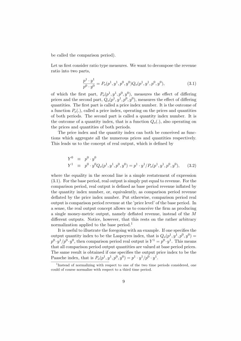
Let us first consider ratio type measures. We want to decompose the revenueratio into two parts,

p1 · y1

p0 · y0= Po(p1, y1, p0, y0)Qo(p1, y1, p0, y0), (3.1)

of which the first part, Po(p1, y1, p0, y0), measures the effect of differingprices and the second part, Qo(p1, y1, p0, y0), measures the effect of differingquantities. The first part is called a price index number. It is the outcome ofa function Po(.), called a price index, operating on the prices and quantitiesof both periods. The second part is called a quantity index number. It isthe outcome of a quantity index, that is a function Qo(.), also operating onthe prices and quantities of both periods.

The price index and the quantity index can both be conceived as func-tions which aggregate all the numerous prices and quantities respectively.This leads us to the concept of real output, which is defined by

Y 0 ≡ p0 · y0

Y 1 ≡ p0 · y0Qo(p1, y1, p0, y0) = p1 · y1/Po(p1, y1, p0, y0), (3.2)

where the equality in the second line is a simple restatement of expression(3.1). For the base period, real output is simply put equal to revenue. For thecomparison period, real output is defined as base period revenue inflated bythe quantity index number, or, equivalently, as comparison period revenuedeflated by the price index number. Put otherwise, comparison period realoutput is comparison period revenue at the ’price level’ of the base period. Ina sense, the real output concept allows us to conceive the firm as producinga single money-metric output, namely deflated revenue, instead of the Mdifferent outputs. Notice, however, that this rests on the rather arbitrarynormalization applied to the base period.1

It is useful to illustrate the foregoing with an example. If one specifies theoutput quantity index to be the Laspeyres index, that is Qo(p1, y1, p0, y0) =p0 ·y1/p0 ·y0, then comparison period real output is Y 1 = p0 ·y1. This meansthat all comparison period output quantities are valued at base period prices.The same result is obtained if one specifies the output price index to be thePaasche index, that is Po(p1, y1, p0, y0) = p1 · y1/p0 · y1.

1Instead of normalizing with respect to one of the two time periods considered, onecould of course normalize with respect to a third time period.

9

Likewise, we want to decompose the cost ratio into two parts,

w1 · x1

w0 · x0= Pi(w1, x1, w0, x0)Qi(w1, x1, w0, x0). (3.3)

the first of which is a price index number and the second a quantity indexnumber. Notice that the functional forms of the price and quantity indicesused to get the decomposition of the revenue ratio, at the output side of thefirm, might differ from the functional forms of the indices used to get thedecomposition of the cost ratio, at the input side of the firm. The first arecalled output indices, and the last input indices.

Real input can now be defined by

X0 ≡ w0 · x0

X1 ≡ w0 · x0Qi(w1, x1, w0, x0) = w1 · x1/Pi(w1, x1, w0, x0), (3.4)

where the equality in the second line is a simple restatement of expression(3.3). For the base period, real input is simply put equal to cost. Forthe comparison period, real input is defined as base period cost inflatedby the input quantity index number, or, equivalently, as comparison periodcost deflated by the input price index number. Put otherwise, comparisonperiod real input is comparison period cost at the ’price level’ of the baseperiod. In a sense, the real input concept allows us to conceive the firm asconsuming a single money-metric input, namely deflated cost, instead of theN different inputs. Notice, however, the normalization involved here.

As defined in the previous chapter, profit is revenue minus cost. Providedthat the base period profit is positive,

p1 · y1 − w1 · x1

p0 · y0 − w0 · x0= (3.5)

Pio(p1, y1, w1, x1, p0, y0, w0, x0)Qio(p1, y1, w1, x1, p0, y0, w0, x0)

would be the desired decomposition of the profit ratio. Since profit dependson inputs as well as outputs, we expect the price and quantity componentsof the profit ratio to depend on input as well as output variables. However,as simple as this desire may be, this is the place where we hit upon anannoying problem. Since profit is a linear function of revenue and cost,it seems natural to express the profit ratio as a linear combination of therevenue ratio and the cost ratio,

10

p1 · y1 − w1 · x1

p0 · y0 − w0 · x0= (3.6)

p0 · y0

p0 · y0 − w0 · x0

p1 · y1

p0 · y0− w0 · x0

p0 · y0 − w0 · x0

w1 · x1

w0 · x0.

Using now expressions (3.1) and (3.3), the profit ratio can be expressed as

p1 · y1 − w1 · x1

p0 · y0 − w0 · x0= (3.7)

p0 · y0

p0 · y0 − w0 · x0Po(p1, y1, p0, y0)Qo(p1, y1, p0, y0)−

w0 · x0

p0 · y0 − w0 · x0Pi(w1, x1, w0, x0)Qi(w1, x1, w0, x0).

This expression, however, does not have the simple multiplicative form (3.5),and it is to be expected that the equivalence of the right hand side of ex-pression (3.7) and the right hand side of expression (3.5) will hold onlyfor specific functional forms. The problem encountered here is due to thesimultaneous occurrence of a ratio and a difference in the profit ratio.

The structure of value added is similar to that of profit. Thus, providedthat the base period value added is positive, the desired decomposition ofthe value added ratio would be

V A1

V A0=p1 · y1 − w1

E · x1E − w1

M · x1M − w1

S · x1S

p0 · y0 − w0E · x0

E − w0M · x0

M − w0S · x0

S

= (3.8)

Pio(p1, y1, w1EMS , x

1EMS , p

0, y0, w0EMS , x

0EMS)×

Qio(p1, y1, w1EMS , x

1EMS , p

0, y0, w0EMS , x

0EMS),

where wtEMS ≡ (wtE , wtM , w

tS) and xtEMS ≡ (xtE , x

tM , x

tS) are the vectors of

prices and quantities of the intermediate inputs. With the first term at theright hand side of this expression we want to capture the contribution ofchanged prices, and with the second term we want to capture the contribu-tion of changed quantities.

Real value added (RVA) can then be defined as

RV A0 ≡ V A0

RV A1 ≡ V A0Qio(p1, y1, w1EMS , x

1EMS , p

0, y0, w0EMS , x

0EMS) (3.9)

= V A1/Pio(p1, y1, w1EMS , x

1EMS , p

0, y0, w0EMS , x

0EMS),

11

that is, comparison period real value added is set equal to value added atthe ’price level’ of the base period. The concept of real value added allows usto see the firm as producing a single output, whose money-metric quantityat period t is given by RV At, from two categories of input, namely capitaland labour.

Using input price and quantity indices, the combined capital and labourcost ratio could be decomposed as

w1K · x1

K + w1L · x1

L

w0K · x0

K + w0L · x0

L

= Pi(w1KL, x

1KL, w

0KL, x

0KL)Qi(w1

KL, x1KL, w

0KL, x

0KL),

(3.10)where wtKL ≡ (wtK , w

tL) and xtKL ≡ (xtK , x

tL) are the vectors of prices and

quantities of the capital and labour inputs. Real capital and labour inputis then defined by

X0KL ≡ w0

K · x0K + w0

L · x0L

X1KL ≡ (w0

K · x0K + w0

L · x0L)Qi(w1

KL, x1KL, w

0KL, x

0KL) (3.11)

= (w1K · x1

K + w1L · x1

L)/Pi(w1KL, x

1KL, w

0KL, x

0KL).

An important, frequently monitored, categorial cost ratio is the labour costratio, w1

L · x1L/w

0L · x0

L. Input price and quantity indices could be used todecompose this ratio as

w1L · x1

L

w0L · x0

L

= Pi(w1L, x

1L, w

0L, x

0L)Qi(w1

L, x1L, w

0L, x

0L). (3.12)

The first part is a labour price index number, and the second part a labourquantity index number. These indices could of course be used to define theconcept of real labour input, Xt

L.

Instead of ratio type measures and their corresponding multiplicative de-compositions, we can opt for difference type measures and additive decom-positions. For example, we now want to decompose the revenue differenceinto two parts,

p1 · y1 − p0 · y0 = Po(p1, y1, p0, y0) +Qo(p1, y1, p0, y0), (3.13)

of which the first, Po(p1, y1, p0, y0), measures the part of the revenue differ-ence that is due to differing prices and the second, Qo(p1, y1, p0, y0), mea-sures the part of the revenue difference that is due to differing quantities.

12

The function Po(.) is called an output price indicator and is assumed to havethe prices and quantities of both periods as arguments. The function Qo(.)is likewise called an output quantity indicator. Notice that both functionsmap price and quantity vectors into money amounts.

A decomposition of the cost difference would be

w1 · x1 − w0 · x0 = Pi(w1, x1, w0, x0) +Qi(w1, x1, w0, x0), (3.14)

where the first component measures the contribution of differing prices andthe second the contribution of differing quantities. Using these functions, the(combined capital and) labour cost difference could be decomposed similarly.

Since profit has by definition a linear structure, for the decomposition ofthe profit difference we can use the two foregoing equations to obtain

(p1 · y1 − w1 · x1)− (p0 · y0 − w0 · x0) =(p1 · y1 − p0 · y0)− (w1 · x1 − w0 · x0) =Po(p1, y1, p0, y0) +Qo(p1, y1, p0, y0)−(Pi(w1, x1, w0, x0) +Qi(w1, x1, w0, x0)) =Po(p1, y1, p0, y0)− Pi(w1, x1, w0, x0) +Qo(p1, y1, p0, y0)−Qi(w1, x1, w0, x0). (3.15)

The first two terms at the right hand side provide the price component,whereas the last two terms provide the quantity component of the profitdifference. Thus, using difference type measures, there appears to be a verysimple relation between the revenue and cost decompositions and the profitdecomposition. A similar relation can easily be derived for the value addeddifference.

It is useful to notice that, although ratio type measures and difference typemeasures can be developed independently, there appears to be a link in thesense that, provided that certain regularity conditions are met, every ratiotype decomposition can be turned into a difference type decomposition andvice versa. The reader is referred to Appendix A for the mathematicaldetails.

What are the advantages and disadvantages of ratio type measures visa vis difference type measures? First of all, a ratio type measure is dimen-sionless and can simply be conceived as 1 plus a percentage change. Forexample,

13

(p1 · y1

p0 · y0− 1

)100% (3.16)

is the percentage change of revenue going from period 0 to period 1, and(Po(p1, y1, p0, y0) − 1)100% is the percentage change of revenue that is dueto price changes. Sometimes, however, one wants to see this change (also)expressed in monetary terms. Then a difference measure is helpful. Thus,p1 · y1− p0 · y0 is the revenue change expressed as an amount of money, andPo(p1, y1, p0, y0) is the part of it that is due to price changes.

Difference measures are advantageous in all situations where the magni-tude that must be decomposed can take on values less than or equal to zero.Then a ratio type measure breaks down, either because dividing by zero isimpossible or because the interpretation of a negative ratio or percentage istroublesome. Examples of magnitudes which can become less than zero are(price and quantity components of) profit and value added.

With some exaggeration, one can say that while economists usually pre-fer ratio type measures, business managers prefer difference type measures.

The important point now is: which formula should be selected as indexor indicator? There are several theoretical approaches available, the mostimportant of which are the axiomatic approach and the economic approach.

The axiomatic approach, with roots in the second half of the 19th cen-tury, specifies requirements which the formulas should satisfy. These re-quirements are called axioms or tests and are usually stated in the formof functional equations. The general idea is that an index or indicator issome kind of average of commodity specific changes. The basic theory forindices can be found in the monograph by Eichhorn and Voeller (1976) andthe review article by Balk (1995). The parallel theory for indicators wasdeveloped by Diewert (1998).

The economic approach, with roots in the first half of the 20th century,combines assumptions on the behaviour of the firm (such as profit maximiza-tion) with assumptions on the prevailing production structure (formulatedin terms of a production function, for instance) to derive empirically imple-mentable formulas for indices and indicators. The basic theory for indicesis outlined by Balk (1998), and for indicators by Balk, Fare and Grosskopf(2000).

Although both approaches lead to a preference for certain specific for-mulas, it is fair to say that they do not lead to the recommendation of asingle formula that could serve all imaginable purposes. If, in the axiomatic

14

approach, the requirements are restricted to those that are more or less self-evident, then quite a number of formulas turn out to be satisfactory. Onthe other hand, every specific formula turns out to be characterized by atleast one property which is not self-evident. With respect to the economicapproach, it turns out that the assumptions needed to justify any specificformula are all more or less subject to argument. Put otherwise, availabletheory makes clear that the choice of a specific formula depends on thepurpose one has in mind.

More important than the theoretical problem of selecting the right for-mula, however, are the many (practical) problems one encounters at thestage of implementation. In addition to those listed in chapter 2, in theintertemporal context the following problems occur:

• The data needed for calculating the theoretically preferred formula arenot timely available, to the effect that a second-best formula must beused. The increasing availability of electronic (scanner) data, however,tends to mitigate this point somewhat.

• The universe of commodities at the input and output side of the firmis not constant but changes continuously. Put otherwise, we have todo with new and disappearing goods and services. In principle, thesecommodities do occur in the value figures of either of the periods whichwe wish to compare, but they become problematic when we proceedto the task of decomposing ratios or differences of those figures.

• Many commodities, especially in the information and communicationtechnology area, undergo a process of more or less rapid quality change.Just comparing quantities and nominal prices does not make muchsense here. It is usually felt that quality change, whether improvementor deterioriation, belongs to the quantity component in a decomposi-tion of revenue or cost change.

All this leads us to expect that actually calculated and published indexnumbers, whether by official agencies or by private organizations, will almostnecessarily exhibit some degree of bias. The problems here are not unlikethose in the field of the Consumer Price Index where the wellknown Boskin etal. (1996) commission report serves as a landmark. The recently completedEurostat (2001) draft Handbook on Price and Volume Measures in NationalAccounts, where the production unit considered is an entire economy, canbe considered as a research agenda. See also Diewert (2001a) for a list ofresearch topics.

15

A prominent place on this research agenda is occupied by the problem ofquantifying quality and variety change. Although over the years statisticalagencies have acquired much experience here and there is an extensive sci-entific literature, a number of theoretical and operational problems are stillwaiting for resolution. Much, but surely not enough, resources are beingspent on the study of hedonic regression techniques. The operational worthof these techniques has for a long time be a topic of debate2, but it seemsthat they are now gradually acquiring a recognized place in the day-to-daywork of statistical agencies.3 Jorgenson (2001) for example remarks that

”The official [i.e. U. S.] price indexes for computers and semi-conductors provide the paradigm for economic measurement.”

The huge literature on methods for dealing with quality and variety changewill be surveyed in the framework of the forthcoming CPI Manual, a jointpublication by Eurostat, ILO, IMF, OECD, UN ECE, and the World Bank.

2See Triplett (1990) for a review of reasons why statistical agencies have resisted he-donic methods.

3These techniques have also found their way into an academic textbook; see Berndt(1991). Berndt and Rappaport (2001) provide a nice summary of work on desktop andmobile personal computers. The latest offspring, result of cooperation between StatisticsNetherlands and the Rotterdam School of Management, is a study by Bode and VanDalen (2001) on passenger cars. This study was presented at the Sixth Meeting of theInternational Working Group on Price Indices (Woolford 2001).

16

Chapter 4

Productivity measures

We are now in a position to discuss what to understand by ’productivity’and ’productivity change’. There appear to be several measures, the mostimportant of which will be reviewed in this chapter.1 The natural startingpoint is to consider the ratio of comparison period and base period prof-itability, that is

p1 · y1/w1 · x1

p0 · y0/w0 · x0. (4.1)

Using relations (3.1) and (3.3), this ratio can be decomposed as

p1 · y1/w1 · x1

p0 · y0/w0 · x0=

p1 · y1/p0 · y0

w1 · x1/w0 · x0=

Po(p1, y1, p0, y0)Pi(w1, x1, w0, x0)

Qo(p1, y1, p0, y0)Qi(w1, x1, w0, x0)

. (4.2)

The index of total factor productivity (TFP), for period 1 relative to period0, is now defined by

ITFP 10 ≡ Qo(p1, y1, p0, y0)Qi(w1, x1, w0, x0)

, (4.3)

which is the real or quantity component of the profitability ratio. Put other-wise, ITFP 10 is the factor with which the output quantities on average havechanged relative to the factor with which the input quantities on averagehave changed. If the ratio of these factors is larger (smaller) than 1, thereis said to be productivity increase (decrease).

1This review follows to some extent the OECD (2001a) Manual.

17

The wording used here suggests that a meaning can be attached to theterm ’productivity’ itself. Let us first consider the purely hypothetical sit-uation of a firm which employs a single input to produce a single output.Then the index of TFP reduces to

ITFP 10 =y1/y0

x1/x0=y1/x1

y0/x0, (4.4)

which has indeed the simple interpretation as a ratio of productivities. Inthe single-input/single-output case yt/xt is the output quantity producedper unit of input quantity, which is a natural measure of the productivityof the production process. In the multi-input/multi-output case the term’productivity’ does not have such a natural sense.

Total factor productivity as a level concept can however be defined as

TFP 0 ≡ p0 · y0/w0 · x0

TFP 1 ≡ (p0 · y0/w0 · x0)ITFP 10. (4.5)

Thus, base period TFP is set equal to base period profitability, and compar-ison period TFP is set equal to base period profitability multiplied by theindex of TFP. Put otherwise, TFP could be called real profitability. Usingthe notation introduced in the previous chapter, we see that base periodTFP can also be expressed as

TFP 0 = Y 0/X0, (4.6)

and that, using again relations (3.1) and (3.3), comparison period TFP canbe expressed as

TFP 1 =p0 · y0Qo(p1, y1, p0, y0)w0 · x0Qi(w1, x1, w0, x0)

=p1 · y1/Po(p1, y1, p0, y0)w1 · x1/Pi(w1, x1, w0, x0)

= Y 1/X1, (4.7)

that is, as real output divided by real input. This is in line with the single-input/single-output case. The relation between the index of TFP and thelevels of TFP is now obviously given by

ITFP 10 = TFP 1/TFP 0, (4.8)

18

but one should be aware of the normalization involved in defining the levelsof TFP. The base period level is normalized as being equal to base periodprofitability.

Using relation (4.2), the TFP index can also be expressed as

ITFP 10 =p1 · y1/w1 · x1

p0 · y0/w0 · x0

Pi(w1, x1, w0, x0)Po(p1, y1, p0, y0)

. (4.9)

The right hand side of this expression consists of two parts. The first part isthe profitability ratio. The second part is the ratio of an input price indexnumber over an output price index number. Thus, if the profitability of thefirm were not changing over time, then TFP change could be measured bythe ratio of an input price index number over an output price index number.Put otherwise, if on average the input prices had increased more (less) thanthe output prices, then TFP change would be larger (smaller) than 1.

In the difference framework, TFP change is measured by the followingindicator:

∆TFP 10 ≡ Qo(p1, y1, p0, y0)−Qi(w1, x1, w0, x0), (4.10)

which is an output quantity indicator minus an input quantity indicator.Notice that TFP change is now measured as an amount of money. Anamount larger (smaller) than 0 indicates TFP increase (decrease).

The index of TFP takes into account all production factors, that is, allinput categories. Traditionally, one speaks of a single factor productivity in-dex when only one input category is taken into account.2 Thus, for instance,the index of labour productivity is defined by

ILP 10 ≡ Qo(p1, y1, p0, y0)Qi(w1

L, x1L, w

0L, x

0L), (4.11)

that is, the ratio of an output quantity index number over a labour inputquantity index number. This is the best known measure of productivitychange. The corresponding level concept, labour productivity, is defined byY t/Xt

L, that is, real output divided by real labour input.

As noticed in the previous chapter, real value added is a frequently usedoutput concept. The corresponding input categories are capital and labour.Thus, the index of value-added-based TFP is defined as the real value addedratio divided by the real capital and labour input ratio,

2One speaks of a multi factor productivity index when more than one input categoryis taken into account.

19

IV ATFP 10 ≡ RV A1/RV A0

X1KL/X

0KL

(4.12)

=Qio(p1, y1, w1

EMS , x1EMS , p

0, y0, w0EMS , x

0EMS)

Qi(w1KL, x

1KL, w

0KL, x

0KL)

,

which is the ratio of a quantity index number of value added and a combinedcapital and labour input quantity index number. The corresponding levelconcept, that is value-added-based TFP, is defined by RV At/Xt

KL.Similarly, the index of value-added-based labour productivity is defined

by

IV ALP 10 ≡ Qio(p1, y1, w1EMS , x

1EMS , p

0, y0, w0EMS , x

0EMS)

Qi(w1L, x

1L, w

0L, x

0L)

, (4.13)

which is the ratio of a quantity index number of value added and a labourinput quantity index number. The corresponding level concept is defined byRV At/Xt

L.

Summarizing, there appear to be at least four different ways of measuringproductivity change and productivity levels. The first main distinction isbetween total factor productivity and single factor productivity. The secondmain distinction is between using the ’natural’, also called gross, outputconcept and the valued added output concept. Moreover, for each of thesefour alternatives there is a ratio and a difference type representation.

Productivity indexes or indicators are extremely important performancemeasures which can be used in a variety of circumstances. Some examplesinclude:

• Tracking the performance of a firm over time.

• Comparing the performance of a certain firm to similar firms, wheresimilarity could be defined with respect to market or production tech-nology.

• Tracking the performance of an aggregate of firms (an industry, oreven the entire economy) over time.

• Comparing the performance of, say, a Netherlands’ industry to thecorresponding industries of other countries.

20

The particular productivity measure that is thereby selected depends on thepurpose of the exercise, the assumptions that can legitimately be made, andthe availability of sufficient data. For an in-depth discussion of the suitabilityof the various measures the reader is referred to the OECD (2001a) Manual.The TFP measure is, by definition, the most general measure of productivitychange.3

Given the definition of the TFP index, expression (4.2) can be simplifiedto

Profitability ratio = ITFP 10 × Po(p1, y1, p0, y0)Pi(w1, x1, w0, x0)

. (4.14)

This expression strongly resembles the Profit Composition Analysis modeldeveloped by the New South Wales Treasury (1999) for analyzing the perfor-mance of regulated firms.4 The second term at the right hand side could becalled the price performance index. It measures the extent to which averageinput price change is recovered by average output price change. Thus, prof-itability change appears to be the combined result of TFP change and priceperformance, and all firms under study could easily be classified into a fourquadrant chart. Moreover, by a slight redefinition of the two period labels,this model could also be used to compare actual profitability to targetedprofitability.

Rearranging expression (4.14) gives

Po(p1, y1, p0, y0) = Profitability ratio × Pi(w1, x1, w0, x0)ITFP 10

. (4.15)

A regulation agency might use this expression as a vehicle for placing abound on the average output price change by restricting the firm’s prof-itability ratio to a prescribed value. Then the allowed rate of change of theoutput prices will be determined by the rate of change of the input pricescorrected by the rate of TFP change. The last rate could be proxied bysome industry- or economy-wide figure.

At the economy level the labour productivity index appears to be aclosely watched statistic, for instance in relation to wage negotiations. More-over, various measures of productivity change play a role in what has come

3The relation between the total factor productivity measures based on the two outputconcepts is discussed, in a production-theoretic framework, by Schreyer (2000).

4The difference is that the PCA model starts with the profit difference instead of theprofitability ratio, and concludes with an expression containing a mixture of ratio typeand difference type measures.

21

to be known as the ”productivity slowdown” discussion. The next chapterprovides some examples.

22

Chapter 5

Two examples

It is useful to present now some recent examples of applied work in this area.I start with a very instructive article by Jorgenson (2001). The productionunit he considers is the U. S. economy. At its output side (Gross Domes-tic Product) he distinguishes between the following categories: investmentgoods, subdivided into non-IT, computers, software, and telecommunica-tions equipment, and consumption goods, subdivided into non-IT goodsand IT capital services. At the input side (Gross Domestic Income) hedistinguishes between capital services, subdivided into non-IT, computers,software, and telecommunications equipment, and labour. His survey illu-minates the challenging problems one encounters in obtaining meaningfulprice and quantity index numbers for all these commodity categories. Inparticular,

”The daunting challenge that lies ahead is to construct constantquality price indexes for custom and own-account software.”

Jorgenson (2001) also remarks that

”As a consequence of the swift advance of information technol-ogy, a number of the most familiar concepts in growth economicshave been superseded. The aggregate production function headsthis list.”

With this statement – in which a mild form of self-criticism might be heard– he draws our attention to the fact that some sectors of modern economiesgrow at a much faster pace than other sectors. When this is the case, it isnot adequate to consider an economy as a ’representative firm’ that produces

23

Table 5.1: TFP change of the U. S. EconomyPeriod Average

yearly percentage1948-1973 0.921973-1990 0.251990-1995 0.241995-1999 0.75

Source: Jorgenson (2001), Table 6.

a single group of outputs. Put otherwise, the selection of a functional formfor an economy’s output quantity or price index should take due account ofthis fact.

Table 5.1 presents some of Jorgenson’s key results. The productivityslowdown, starting in the seventies, is clearly depicted as is the resurgenceoccurring in the second half of the nineties. Contrary to folk wisdom heconcludes that this resurgence stems not only from the IT sectors of theeconomy but to an important degree also from the non-IT sectors. Theexplanation, however, appears to be still outstanding. Therefore, Jorgensonconcludes that

”Top priority must be given to identifying the impact of invest-ment in IT at the industry level.” and

”The next priority is to trace the increase in aggregate TFPgrowth to its sources in individual industries.”

An other nice illustration is provided by a recent publication of TheConference Board (McGuckin and Van Ark 2001). This publication, entitled”Performance 2000: Productivity, Employment, and Income in the World’sEconomies”, highlights the differences between some thirty economies overthe last decade. This is an example of a comparison in a combined timeseries/cross-section (panel) framework. The additional layer of complexityis caused by the fact that prices not only change over time but also differbetween the economies. Price differences between economies are capturedby, what traditionally are called, purchasing power parities.1

The measure used in this publication is labour productivity, defined asGDP per hour worked. All value figures are converted with purchasing

1A recent survey of the theory of international price and quantity comparisons wasprovided by Balk (2001).

24

Table 5.2: Labour productivity changeAverage yearly percentage

1990-1995 1995-2000U. S. A. 0.8 2.6E. U. 2.4 1.2OECD 1.7 2.0Netherlands 1.0 1.4

Source: McGuckin and Van Ark (2001), Table 2.

power parities to the U. S. 1996 price level. The differences in performance,summarized in Table 5.2, are striking. Again, the question is, what is lyingbehind those aggregate figures?

25

Chapter 6

Some history

Interesting details on the history of the concept of (total factor) productivitychange can be found in Griliches (2001), the first chapter of which is areworked version of his 1996 article on ”the discovery of the residual.”

The first mention of TFP change as the ratio of an output quantity indexand an input quantity index occurs in a contribution by Copeland (1937)in what, with hindsight, could be called the national income accountingapproach. Stimulated by institutions such as the NBER, in the post-warperiod several studies were published, a typical one being Stigler (1947).These studies were mainly dealing with industry- or economy-wide aggre-gates. Although the TFP index was sometimes referred to as a measure ofthe efficiency of the economic process, the common opinion was best voicedby Abramowitz (1956), who called it a ”measure of our ignorance.”1

The other, production-theoretic approach appears to go back to Tin-bergen (1942). He extended the Cobb-Douglas production function with atime trend variable. The difference between the growth rate of real outputand a weighted average of the growth rates of real capital and labour in-put was interpreted variably as efficiency change, technical development, or”Rationalisierungsgeschwindigkeit”.

The basic and very influential contribution of Solow (1957) can be con-ceived as some sort of linkage of both traditions. He showed that undercertain conditions the parameters of the Cobb-Douglas production functioncould be equated to observable statistical magnitudes and the residual inter-preted in terms of a ratio of output and input quantity index numbers. This

1This has become a frequently repeated quote, the latest variation being Lipsey andCarlaw’s (2001) conclusion that ”TFP is as much a measure of our ignorance as it is ameasure of anything positive.”

26

is why the TFP index came to be known as the ”Solow residual”, althoughthe name ”residual” appears to have been used by Domar (1961) for thefirst time. Solow interpreted the residual as a measure of technical change.

Since the inception of the concept of TFP change there have been twomain styles of research. The first was directed at explanation. The secondwas directed at better measurement, primarily of the input factors capitaland labour. In the beginning, the second style was more prominent than thefirst. For example, Jorgenson and Griliches (1967) claimed that using the”correct” index number framework and the ”right” measurement of inputswould largely eliminate the role of the residual.

The residual disappeared indeed, but not at all due to better measure-ment techniques. The economy-wide disappearance of productivity growthin the seventies, its reappearance later on, and the search for the factorsbehind this world-wide phenomenon came to be known as the ”productivityslowdown discussion”. The emphasis shifted from measurement problemsto explanation, and Griliches’ work provides a clear demonstration of thisshift. The main explanatory factors he considered were the role of educationand R&D expenditures.

The measurement problems, however, remained important. Lookingback at a life-long of research in this area, Griliches (2001) says:

”It is my hunch that at least part of what happened [namely,the productivity slowdown] is that the economy and its varioustechnological thrusts moved into sectors and areas in which ourmeasurement of output are especially poor: services, informationactivities, health, and also the underground economy.”

but at the end of the day he concludes that

”There have been many reasonable attempts to explain the pro-ductivity slowdown (...), but no smoking gun has been found,and no single explanation appears to be able to account for allthe facts, leaving the field in an unsettled state until this day.”

Until the nineties, the research on productivity change typically made use ofthe concept of the ”representative firm” in combination with aggregate em-pirical material provided by statistical agencies. The increased availabilityof longitudinal enterprise microdata sets has opened up many new, excitingresearch possibilities.2 Researchers are by now able to track large numbers

2See for instance McGuckin (1995) or Heckman’s (2001) Nobel Lecture.

27

of individual firms over time. This has led to a completely new area ofresearch, with its own conferences3 and research centers.4

3The international conferences on Comparative Analysis of Enterprise (micro)Data(Helsinki 1996, Bergamo 1997, The Hague 1999, Aarhus 2001) and the International Sym-posium on Linked Employer-Employee Data (Arlington VA 1999).

4These (usually confidential) microdata sets mainly originate from databases underly-ing aggregate figures published by national statistical agencies. They are, a.o., availablefor researchers at the Center for Economic Studies of the U. S. Bureau of the Census andthe Center for Research of Economic Microdata (Cerem) of Statistics Netherlands.

28

Chapter 7

Explaining aggregateproductivity change

The explanation of aggregate productivity change, that is, productivitychange at the level of an industry or an economy, starts with the truismthat any aggregate is made up from a (large) number of individual firms.The relation between aggregate productivity change and firm-specific pro-ductivity change is, however, not a simple one. Though any aggregate can beconceived as a super-firm, and the same basic measurement model is appli-cable to aggregates and individual firms, such a super-firm is not the simplesum of a number of individual firms. In explaining aggregate productivitychange we must not only deal with the temporal dynamics of the relevantpopulation of firms, but also with the fact that these firms possibly interactwith each other via transactions in goods and services. As will appear inthis chapter, the dynamics has got a great deal of attention over the lastyears. The interaction, however, is a largely unexplored issue.1

Sidestepping the interaction issue, the two main factors contributing toaggregate productivity change are intra-firm productivity change, and inter-firm reallocation. This reallocation is caused by the dynamic process of firmexpansion, contraction, entry and exit. The first question, thus, is whetherit is possible to distinguish unequivocally between all those factors.

As in the foregoing we will consider two periods. The set of firms ex-isting at both periods will be denoted by C (continuing firms). The set offirms existing at the base period but no more at the comparison period willbe denoted by X (exiting firms), and the set of firms born after the base

1The basic reference on the relation between aggregate and individual measures ofproductivity change still being Domar (1961).

29

period and still existing at the comparison period will be denoted by N (en-tering firms). The productivity level (according to one of the four versionsdiscussed in chapter 4) of firm i at period t will be denoted by PRODit.Each firm comes with some measure of relative size (based on the value ofoutput or employment) in the form of a weight θit. These weights add upto 1 for each period, that is∑

i∈C∪Nθi1 =

∑i∈C∪X

θi0 = 1. (7.1)

The aggregate productivity level at period t is defined as the weighted aver-age of the firm-specific productivity levels2, that is PRODt ≡

∑i θitPRODit,

where the summation is taken over all firms existing at period t. Aggregateproductivity change between periods 0 and 1 is then given by

PROD1 − PROD0 =∑

i∈C∪Nθi1PRODi1 −

∑i∈C∪X

θi0PRODi0. (7.2)

This can initially be decomposed as

PROD1 − PROD0 =∑i∈N

θi1PRODi1

+∑i∈C

θi1PRODi1 −∑i∈C

θi0PRODi0

−∑i∈X

θi0PRODi0. (7.3)

The first term at the right hand side shows the contribution of enteringfirms, the second and third term together show the contribution of continu-ing firms, whereas the last term shows the contribution of exiting firms. Thecontribution of continuing firms is the outcome of an interaction betweenintra-firm productivity change, PRODi1−PRODi0, and inter-firm relativesize change, θi1 − θi0. There have been developed several methods to de-compose this contribution further. We will review the various possibilities.

The first method decomposes the contribution of the continuing firmsinto a Laspeyres-type contribution of intra-firm productivity change and aPaasche-type contribution of relative size change:

2For an analysis in terms of firm-specific productivity changes the reader is referred toAppendix B.

30

PROD1 − PROD0 =∑i∈N

θi1PRODi1

+∑i∈C

θi0(PRODi1 − PRODi0) +∑i∈C

(θi1 − θi0)PRODi1

−∑i∈X

θi0PRODi0. (7.4)

The second term at the right hand side relates to intra-firm productivitychange and uses base period weights. It is therefore called a Laspeyres-typemeasure. The third term relates to relative size change and is weighted bycomparison period productivity levels. It is therefore called a Paasche-typemeasure. This decomposition was used in the study of Baily et al. (1992).

It is, however, equally defendable to use a Paasche-type measure forintra-firm productivity change and a Laspeyres-type measure for relativesize change. This leads to a second decomposition, namely

PROD1 − PROD0 =∑i∈N

θi1PRODi1

+∑i∈C

θi1(PRODi1 − PRODi0) +∑i∈C

(θi1 − θi0)PRODi0

−∑i∈X

θi0PRODi0. (7.5)

It is possible to avoid the choice between the Laspeyes-Paasche-type andthe Paasche-Laspeyres-type decomposition. The third method uses for thecontribution of both intra-firm productivity change and relative size changeLaspeyres-type measures. However, this simplicity is counterbalanced bythe necessity to introduce a covariance-type term:

PROD1 − PROD0 =∑i∈N

θi1PRODi1

+∑i∈C

θi0(PRODi1 − PRODi0) +∑i∈C

(θi1 − θi0)PRODi0

31

+∑i∈C

(θi1 − θi0)(PRODi1 − PRODi0)

−∑i∈X

θi0PRODi0. (7.6)

Due to the fact that the base period and comparison period weights add upto 1, we can insert an arbitrary scalar a, to obtain

PROD1 − PROD0 =∑i∈N

θi1(PRODi1 − a)

+∑i∈C

θi0(PRODi1 − PRODi0) +∑i∈C

(θi1 − θi0)(PRODi0 − a)

+∑i∈C

(θi1 − θi0)(PRODi1 − PRODi0)

−∑i∈X

θi0(PRODi0 − a). (7.7)

In view of the Laspeyres-type perspective, a natural choice for a seems tobe PROD0, the base period aggregate productivity level. This leads to thedecomposition proposed by Haltiwanger (1997).

Instead of using the Laspeyres perspective, one might use the Paascheperspective. The covariance-type term accordingly appears with a negativesign. Thus, the fourth decomposition is

PROD1 − PROD0 =∑i∈N

θi1(PRODi1 − a)

+∑i∈C

θi1(PRODi1 − PRODi0) +∑i∈C

(θi1 − θi0)(PRODi1 − a)

−∑i∈C

(θi1 − θi0)(PRODi1 − PRODi0)

−∑i∈X

θi0(PRODi0 − a). (7.8)

The natural choice for a would now be PROD1, the comparison periodaggregate productivity level.

The fifth method avoids the Laspeyres-Paasche dichotomy altogether, byusing the symmetric method due to Bennet (1920). This symmetry obviatesthe need for a covariance-type term too. Thus,

32

PROD1 − PROD0 =∑i∈N

θi1PRODi1

+(1/2)∑i∈C

(θi1 + θi0)(PRODi1 − PRODi0)

+(1/2)∑i∈C

(θi1 − θi0)(PRODi1 + PRODi0)

−∑i∈X

θi0PRODi0. (7.9)

We can again insert an arbitrary scalar a, to obtain

PROD1 − PROD0 =∑i∈N

θi1(PRODi1 − a)

+(1/2)∑i∈C

(θi1 + θi0)(PRODi1 − PRODi0)

+(1/2)∑i∈C

(θi1 − θi0)(PRODi1 + PRODi0 − 2a)

−∑i∈X

θi0(PRODi0 − a). (7.10)

A rather natural choice for a is now (PROD1 + PROD0)/2, the averageaggregate productivity level. Substituting this in the last expression andrearranging somewhat, we finally get

PROD1 − PROD0 =∑i∈N

θi1(PRODi1 − PROD1 + PROD0

2)

+∑i∈C

θi1 + θi0

2(PRODi1 − PRODi0)

+∑i∈C

(θi1 − θi0)(PRODi1 + PRODi0

2− PROD1 + PROD0

2)

−∑i∈X

θi0(PRODi0 − PROD1 + PROD0

2). (7.11)

33

Thus, entering firms contribute positively to aggregate productivity changeif their productivity level is above average. Similarly, exiting firms contributepositively if their productivity level is below average. Continuing firms cancontribute positively in two ways: if their productivity level increases, or ifthe firms with above (below) average productivity levels increase (decrease)in relative size. This decomposition is closely related to the one used byGriliches and Regev (1995). In view of its symmetry it should be the pre-ferred one. Moreover, Haltiwanger (2000) notes that (7.11) is apt to be lesssensitive to (random) measurement errors than (7.7).

This overview demonstrates a number of things. First, there is no uniquedecomposition of aggregate productivity change as defined by expression(7.2). Second, one should be careful with reifying the different components,in particular the covariance-type term, since this term can be consideredas being an artifact arising from the specific (Laspeyres- or Paasche-) per-spective chosen. Third, the undetermined character of the scalar a lendsadditional arbitrariness to these decompositions. Thus, it is to be expectedthat the outcome of any decomposition exercise will depend to some extenton the particular expression favoured by the researcher.

Having done with these, not unimportant, formalities it is time to presentan illustration. We do this by drawing on some results obtained by a teamof national experts in a project of the Economics Department of the OECD.The novel feature of this project is that a common analytical frameworkwas used on sets of longitudinal enterprise microdata from a number ofmember states. These data sets were, to the extent possible, harmonized.Most results obtained sofar are for total manufacturing. Table 7.1 presentsthe outcomes for aggregate labour productivity change. The decompositionmethod used is that of expression (7.11), whereas the shares are based onemployment.

It appears that there are substantial differences between the annual per-centage changes of aggregate labour productivity over the countries. Thisapplies to both five yearly intervals. Further, entering and exiting firmsappear to have a large influence. Sometimes the contributions of entry andexit go in the same direction, sometimes they go in opposite directions.Moreover, there appears to be a fair amount of reallocation between firms,the effect of which can go in either direction. However, by and large theintra-firm productivity change component tends to dominate the picture.3

The question thus shifts to the factors determining the intra-firm pro-ductivity changes. This has become an area of vigorous research, facilitated

3Limited information suggests that this is less so in the case of TFP.

34

Table 7.1: Decomposition of labour productivity change, total manufactur-ing

Annual Percentage share of each componentpercentage Entry Within Between Exit

1985-1990Finland 5.4 0.4 72.5 7.0 20.1France 2.0 -20.2 84.7 1.9 33.6Italy 4.8 10.7 62.1 9.0 18.3Netherlands 1.5 33.5 99.9 -8.1 -25.2Portugal (1987-91) 6.6 -13.4 91.4 -9.7 31.8United Kingdom 1.6 13.7 98.3 -7.4 -4.6United States (1987-92) 1.6

1990-1995Finland (1989-94) 4.6 -2.5 68.4 16.1 18.0France 0.0W. Germany (1992-97) 2.1 -0.7 115.3 -12.1 -2.6Italy 5.5 15.7 58.2 7.0 19.1Netherlands 2.8 20.5 78.2 -10.8 12.1Portugal 6.8 5.3 62.6 -4.3 36.4United Kingdom (1987-93) 1.7 8.8 59.9 3.1 28.2United States (1992-97) 3.0Source: OECD (2001b), Figure VII.1. Numerical figures from Scarpetta et al.(2001).

by the opportunities to link production survey type data to data comingfrom other kinds of firm level surveys, such as the Community InnovationSurveys or the Wage Structure Surveys. There are some excellent reviewpapers which summarize the results obtained sofar: Bartelsman and Doms(2000), Haltiwanger (2000), and Ahn (2001), of which the last is the mostcomprehensive.

What are the main empirical findings? Bartelsman and Doms (2000)summarize the lessons as follows:

”First, the amount of productivity dispersions is extremely large– some firms are substantially more productive than others. Sec-ond, highly productive firms today are more than likely to behighly productive firms tomorrow, although there is a fair amountof change in the productivity distribution. Third, a large por-tion of aggregate productivity growth is attributable to resourcereallocation. The manufacturing sector is characterized by largeshifts in employment and output across establishments every

35

year – the aggregate data belie the tremendous amount of tur-moil underneath. This turmoil is a major force contributingto productivity growth, resurrecting the Schumpeterian idea ofcreative-destruction. Fourth, quantifying the importance of var-ious factors behind productivity growth, such as changes in theregulatory environment or changes in technology, is a difficulttask and has been only partially successful. Nonetheless, someuseful lessons have been learned. In terms of the regulatory en-vironment, any regulations that inhibit resource reallocation canhave detrimental effects on productivity growth. Regarding theeffect of technology on productivity, it is now known that docu-menting the correlation between a factor of production, such ascomputers, and productivity is not enough to understand causalmechanisms. Use of computers also is related to other variablescorrelated with productivity, such as human capital and man-agerial ability.”

After reviewing quite a number of studies on productivity correlates suchas regulation, management/ownership, technology and human capital, andinternational exposure, their conclusion is that

”At the micro level, productivity remains very much a measureof our ignorance.”

Ahn’s (2001) conclusion is also worthwhile to quote here in full:

”Both technology and human capital of workers appear to in-fluence firm-level productivity. Innovative firms tend to shiftthe composition of their labour force toward more skilled labourthrough recruiting and training, and such shifts are often ac-companied by higher productivity and higher wages for skilledlabour.

A direct causal link between technology or human capital andproductivity at the individual level is difficult to prove, whileevidence of technology-skill complementarity is widely observed.Both advanced technology use and higher wages may well be aresult of a third factor (e.g. better management).

Findings from micro data suggest that ownership structure isan important determinant of firm-level productivity. Likewise,

36

exposure to competition, including international trade, plays avery important role in selecting high productivity firms.

There are large and persistent differences in productivity levelsacross producers even in the same industry, and inputs and out-puts are constantly reallocated from less efficient ones to moreefficient ones through firm dynamics. Aggregate productivitygrowth comes from firm dynamics as well as from within-firmproductivity growth.

The contribution of firm dynamics to aggregate productivityappears to be more pronounced for total factor productivitygrowth than for labour productivity growth. While within-firmproductivity growth seems to drive overall fluctuations in ag-gregate productivity growth, the contribution from the exit oflow-productivity units increases its importance during cyclicaldownturns.

In spite of the large and still increasing share of the service sectorin most OECD countries, difficulties in measuring service pro-ductivity have obliged most studies on firm dynamics and pro-ductivity growth to be focused on manufacturing. Emerging em-pirical studies suggest that firm dynamics are more volatile andmore important for explaining aggregate productivity growth inthe service sector than in the manufacturing sector.”

The basic problem with measuring productivity change in the service sectoris the unavailability of suitable price index numbers. It is therefore of utmostimportance that statistical agencies try to close this gap.

37

Chapter 8

What is productivitychange?

As we have seen in the foregoing, several suggestions have been offered as ananswer to the question: what is productivity change? In this chapter we willtake a closer look at the meaning of productivity change at the individualfirm level.

Measuring productivity change over time or comparing productivity lev-els between entities starts with positing something that is stable and/orcommunal. We will call this the technology and suppose that it is sharedby at least the set of firms we wish to compare.

The classical approach was to represent the technology by a productionfunction and to assume that all firms are behaving optimally in some eco-nomic sense, that is, for instance, as being profit-maximizers. The progressof the last two decades was brought about by recognizing the heterogeneityof reality, in the sense i) that the technology is a set rather than a function,and ii) that firms might behave non-optimally.

We will first illustrate the concept of TFP by a simple picture and thenproceed to a discussion of the various factors which contribute to TFPchange. We will thereby employ the various concepts defined in chapters3 and 4.

The horizontal axis in Figure 8.1 measures real input, whereas the ver-tical axis measures real output. Both are, as noticed earlier, conditionalon a certain normalization with respect to input-mix and output-mix re-spectively. Put otherwise, the picture represents a single ’slice’ of the fullN +M -dimensional space of input and output quantities.

The technology of period t is to be thought of as the body of both tacit

38

- X

6

Y

St

q a = (Xt, Y t)

��������

q b

Figure 8.1: Total Factor Productivity

and explicit knowledge concerning products, processes, and organizationalstructures. Based on this body of knowledge there is a set of feasible com-binations of input quantities and output quantities. In Figure 8.1 this set isrepresented by the area bounded by the curved line and the horizontal axis.As depicted here, this set is assumed to exhibit some simple properties likefree disposability of inputs and outputs. In reality, however, this set mighthave a less simple form.

The boundary of the technology set, that is the curved line itself, iscalled the frontier. This name is very appropriate, since beyond the frontierlie all those input-output combinations that are infeasible according to thetechnological state of affairs in period t. The mathematical representationof the frontier is the familiar production function Y = F t(X).

Each individual firm occupies a certain point within the technology set.Two examples have been drawn in the figure. The firm at point a uses realinput Xt and produces real output Y t. The TFP of this firm is then given

39

by the ratio Y t/Xt, which is just equal to the slope of the line connectingthe origin O with the point a. Expanding real input Xt and real outputY t with the same factor will leave TFP unchanged. Every other change ininput or output quantities will in principle lead to TFP change. We willdiscuss now the various factors by which TFP can change.

As depicted, firm a is not particularly efficient. For instance, holdingits real input Xt constant, the firm could expand its real output Y t bya certain factor until it reaches the frontier. Or, holding its real outputY t constant, it could contract its real input Xt by a certain factor untilit reaches the frontier. Put otherwise, the firm can increase its efficiencyby moving towards the frontier in the NW direction. This means that theslope of the line Oa increases, which is tantamount to saying that increasingefficiency means increasing TFP.

Consider now firm b. Since, as depicted, this firm is acting on the frontier,it is technically efficient. However, its TFP, that is the slope of the line Ob,can still change by moving on the frontier. There appear to be two logicallydistinct types of movement here:

1. The first is a movement within the ’slice’ of the quantity space asdrawn in the picture, that is a movement conditional on the firm’s input-and output-mix. In particular, the firm could move towards the point wherethe slope of Ob attains its maximal value. This point would be reached whenthe line Ob became tangential to the frontier. At that point the firm’s TFPwould be maximal. This is what we will call the scale effect. The scale effectdepends of course on the curvature of the frontier. Imagine, for instance,that the frontier is a straight line originating at O. Then a movement offirm b along this line would not change its TFP.

2. The firm can also move on the frontier by adapting its input- oroutput-mix. This type of movement can of course not be represented inour simple figure since it cuts across all dimensions of the quantity space.Adaptation of the firm’s input-mix can, for instance, be caused by a re-laxation of capacity restrictions. Also, by moving towards the point wherethe firm is considered to be economically optimal, that is, the point wherethe firm, given the prices of all the inputs and outputs, maximizes profit,causes the input- or output-mix to change. At such a point the firm is calledallocatively efficient.

Finally, the frontier itself can change over time. This means that thetechnology set changes, and is therefore called technological change.1 An

1To be precise, this should be called disembodied technological change. Technologicalchange as embodied in any input category is taken care of by the quality adjustment that

40

outwardbound change of the frontier is usually associated with technologicalprogress, whereas an inwardbound change is associated with technologicalregress. These changes can be of local nature, which means that a certainregion can exhibit progress while an other region can exhibit regress. As-suming that our firm continues to stay on the frontier, technological changebrings about TFP change.

It may be clear that, in order to arrive at measurement, all these ratherintuitive notions must be made precise. The instruments needed in the firstplace are provided by duality theory.2 Starting with the notion of a technol-ogy set St, duality theory shows that there are quite a number of equivalentrepresentations of such a set in the form of mathematical functions. Themain distinction thereby is between distance functions and value functions.Distance functions act on (primal) quantity space and are dimensionless.Value functions act on (dual) price space and have the money dimension.Well known among the distance functions are the (radial) input- and out-put distance functions. Well known among the value functions are the cost,revenue, and profit functions.

Let us try to make this a little bit more specific, without introducing toomuch mathematical detail. For this, the reader is referred to the literature.3

We first discuss some output-orientated measures. The (direct) outputdistance function is defined by

1/Dto(x, y) ≡ sup{δ | δ > 0, (x, δy) ∈ St}. (8.1)

The right hand side of this expression looks for the largest factor δ by whichthe output quantity vector y can be multiplied such that the resulting quan-tity vector δy is still producible by the input quantity vector x. The inverseof this largest factor is called the output distance function. This functionis a (radial) measure of technical efficiency, which attains values between 0and 1, conditional on a certain input quantity vector x and the output-miximplied by y.

The (direct) revenue function is defined by

Rt(x, p) ≡ maxy{p · y | (x, y) ∈ St}, (8.2)

must be made in order to make any ’new’ input comparable to an ’old’ input in quantityterms. See Lipsey and Carlaw (2001) for more on this issue.

2See Fare and Primont (1995).3See also the excellent, non-technical overview by Lovell (2000) with references to the

more technical literature.

41

that is, the maximum revenue that can be obtained when output prices aregiven by p and the input quantities are fixed at x.

The indirect functions replace the conditioning input quantity vector bya budget constraint together with an input price vector. Thus, the indirectoutput distance function, defined by

1/IDto(w/c, y) ≡ sup{δ | δ > 0, (x, δy) ∈ St, w · x ≤ c}, (8.3)

is again a measure of technical efficiency, based on the output-mix of y,but now conditional on the set of input quantity vectors which satisfy therequirement that their cost w ·x does not exceed a given budget c. Likewise,the indirect revenue function is defined by

IRt(w/c, p) ≡ maxy{p · y | (x, y) ∈ St, w · x ≤ c}, (8.4)

that is, the maximum revenue that can be obtained when output prices aregiven by p and the input quantities are such that their cost at input pricesw does not exceed the budget c.

For the input orientation a similar set of measures exist. The (direct)input distance function is formally defined by

1/Dti(x, y) ≡ inf{δ | δ > 0, (δx, y) ∈ St}. (8.5)

At the right hand side we now look for the smallest factor δ by which theinput quantity vector x can be multiplied such that δx is still able to producethe output quantity vector y. The inverse of this smallest factor is called theinput distance function. The right hand side of the last expression itself isa measure of technical efficiency, conditional on the output quantity vectory and the input-mix given by x.

The (direct) cost function is defined by

Ct(w, y) ≡ minx{w · x | (x, y) ∈ St}, (8.6)

that is, the minimum cost that is necessary for producing the output quan-tities y when input prices are given by w.

The indirect functions replace the conditioning output quantity vectorby a revenue target together with an output price vector. Thus, the indirectinput distance function, defined by

1/IDti(x, p/r) ≡ inf{δ | δ > 0, (δx, y) ∈ St, p · y ≥ r}, (8.7)

42

is again an inverse measure of technical efficiency based on x’s input-mix,but now conditional on the set of output quantity vectors which satisfy therequirement that their revenue p · y is not less than a prescribed target r.Likewise, the indirect cost function is defined by

ICt(w, p/r) ≡ minx{w · x | (x, y) ∈ St, p · y ≥ r}, (8.8)

that is, the minimum cost that is necessary, under input prices w, to yieldrevenue r when output prices are given by p.

Finally, the profit function is defined by

Πt(w, p) ≡ maxx,y{p · y − w · x | (x, y) ∈ St}, (8.9)

that is, the maximum profit that can be obtained when output prices are pand input prices are w.

The fact that, without additional specifications, all these functions4 rep-resent the same technology enables the analyst to choose the analyticalframework that fits 1) the behavioural objective that is assigned to or con-sidered appropriate for the firms studied, and 2) the data available. Forinstance, suppose that the firms studied can be considered to be compet-itive profit maximizers, but that, for some reason, the analyst has onlydata on input prices and output quantities. Then an analysis in terms ofthe cost function is still appropriate, since profit maximization implies costminimization.

By using these functions it is possible to replace the intuitive notions oftechnological change, technical efficiency change, allocative efficiency change,scale efficiency change, and input- or output-mix change by precisely formu-lated expressions which are adapted to the situation under study. Moreover,within the various frameworks it is possible to formulate hypotheses, for in-stance about the nature of technological change or about the scale propertiesof a technology.

The first question we now want to address is how these theoretical measuresrelate to the conventional, data-driven measures as discussed in chapter 4.This is among the main subjects of Balk’s (1998) monograph. The resultsappear to be limited in scope.

One of the basic theoretical measures is what came to be called, dueto Caves, Christensen and Diewert (1982), the (primal) Malmquist produc-

4In addition to the nine functions considered here, there are nonradial distance func-tions and various kinds of conditional distance and value functions.

43

tivity index.5 By construction this index, which is defined as a function of(direct or indirect, input or output) distance functions, captures technologi-cal change and technical efficiency change. Put another way, it captures themovement of the frontier as well as the firm’s position relative to the fron-tier. Using various assumptions, it appears possible to relate this theoreticalproductivity index to an index of the form (4.3).

Specifically, one has to assume that the technology can be represented bya suitable6 functional form which changes through time in a ’smooth’ way;that the technology exhibits (locally) constant returns to scale; that thefirm is and remains allocatively efficient, which means that, depending onthe orientation chosen, its input-mix or output-mix is and remains optimal;that the firm, conditional on its input- or output-orientated technical effi-ciency, competitively maximizes profit. Under this assumptions it turns outthat, depending on the specific functional form chosen, the Malmquist pro-ductivity index reduces either to the ratio of a Fisher output quantity indexand a Fisher input quantity index or to the ratio of an (explicit or implicit)Tornqvist output quantity index and an (explicit or implicit) Tornqvist in-put quantity index.

Put otherwise, given all those assumptions, the TFP index appears tocapture the combined effect of technological change and technical efficiencychange. If one also were to assume that the firm is and remains technicallyefficient – which implies that the firm is cost efficient –, then the TFP indexreduces to a measure of technological change. The whole set of assumptionsleading up to this result – briefly summarized: a constant-returns-to-scaletechnology and a competitively profit-maximizing firm – reflects the classicalposition.

It may be clear that this position is not very realistic. Although onecould argue that the assumption of constant returns to scale can validlybe made on a global level and for the long run, it appears to be hardlytenable on a sectoral level and for the short run. And there is also sufficientevidence that firms are not behaving as nicely as theory would like themto do. However, any relaxation of assumptions comes at a price. We mustinvoke econometric methods in order to proceed.

Econometric methods are in the first place needed to estimate, within theframework chosen for the analysis, the function which represents the tech-nology set St. Suppose that we have data (xit, yit) on firms i = 1, ..., I.

5For some history related to this concept see Grosskopf (2001).6The word ’suitable’ could be used as a hyperlink to a whole body of theoretical results

on flexible functional forms.

44

There are a number of techniques available. The first we briefly consider isthe method of activity analysis.

The basic idea of this method is that every pair (xit, yit) (i = 1, ..., I) –that is, every observed activity – is an element of the set St. Thus St can beapproximated by enveloping the observations as closely as possible – hencethe alternative name Data Envelopment Analysis (DEA) – by piecewiselinear contours. We consider two of those approximations. The first one,

St(CRS) ≡ {(x, y) |I∑

i′=1

zi′xi′t ≤ x, y ≤

I∑i′=1

zi′yi′t, (8.10)

zi′ ≥ 0 (i′ = 1, ..., I)},

imposes globally constant returns to scale. The second one,

St(V RS) ≡ {(x, y) |I∑

i′=1

zi′xi′t ≤ x, y ≤

I∑i′=1

zi′yi′t, (8.11)

zi′ ≥ 0 (i′ = 1, ..., I),I∑

i′=1

zi′ = 1},

admits variable returns to scale. Since the addition of a restriction reducesthe set of feasible elements, we have

St(V RS) ⊆ St(CRS), (8.12)

that is, St(V RS) envelops the data more closely than St(CRS).Based on these approximations, any input distance function value can

be computed by solving the following linear programming problem

1/Dti(x, y) = min

z,δδ subject to (8.13)

I∑i′=1

zi′xi′t ≤ δx, y ≤

I∑i′=1

zi′yi′t,

zi′ ≥ 0 (i′ = 1, ..., I), [I∑

i′=1

zi′ = 1],

and any cost function value can be computed by solving the following linearprogramming problem

45

Ct(w, y) = minz,x

w · x subject to (8.14)

I∑i′=1

zi′xi′t ≤ x, y ≤

I∑i′=1

zi′yi′t,

zi′ ≥ 0 (i′ = 1, ..., I), [I∑

i′=1

zi′ = 1].

The restriction between brackets in these two equations must of course bedeleted in the case of imposing globally constant returns to scale.

For the other functions reviewed above similar linear programming prob-lems could be stated. I refer to Fare, Grosskopf and Lovell (1994) for adetailed exposition of the theory. A useful reader on theory as well as appli-cations is Charnes, Cooper, Lewin and Seiford (1994). A more recent sourceis Cooper, Seiford and Tone (1999). There have been developed a number of(semi-) commercial software packages, such as Warwick DEA Software (seewww.deazone.com), Frontier Analyst (see www.banxia.com), and On Front(see www.emq.se) to execute the necessary calculations.

The second technique is called stochastic frontier analysis (SFA). The basicidea behind this technique, or rather this set of techniques, can most easilybe grasped by first considering the conventional approach.

Suppose that the firms under study could be considered as competitivecost minimizers, facing the same prices. This means that, for each firm i(i = 1, ..., I), its actual cost cit ≡ wt · xit is equal to the minimum costas given by the cost function, Ct(wt, yit). Since the actual form of the costfunction is unknown, Ct(w, y) must be replaced by a suitable functional formf(w, y, t; Φ), where Φ denotes a set of unknown parameters. A stochasticnoise term is added, and Φ is to be estimated from a set of equations like

ln cit = ln f(wt, yit, t; Φ) + vit (i = 1, ..., I). (8.15)

The stochastic noise term is thereby usually assumed to be independent andidentically distributed according to a normal distribution with mean zero.

Stochastic frontier analysis explicitly recognizes the fact that firms mightnot behave optimally. In the present example this means that actual cost cit

may be higher than minimum cost Ct(wt, yit), but never can be lower. Thiscan be modelled by introducing an additional, asymmetrically distributedterm, and replacing (8.15) by

46

ln cit = ln f(wt, yit, t; Φ) + uit + vit (i = 1, ..., I). (8.16)

In this system of equations, as before, vit represents noise and is accordinglydistributed symmetrically around zero. But uit represents inefficiency, isalways non-negative, and must therefore follow an asymmetrical distribution(usually a truncated-at-zero normal distribution). Both terms are assumedto be independently distributed.

The foregoing paragraphs were only intended to give an idea of the ap-proach pursued by stochastic frontier analysts.7 The main features distin-guishing SFA from DEA might, however, be clear. Whereas SFA is basicallya regression method, yields a smooth frontier, is stochastic, and parametric,DEA is based on solving linear programming problems, yields a piecewiselinear frontier, is deterministic, and nonparametric.

Since its inception, a quarter of a century ago, the body of theory andapplications relating to SFA has grown almost exponentially. The stateof the art was recently reviewed by Kumbhakar and Lovell (2000). Coelli(1996) developed a non-commercial software package for stochastic frontierestimation.

The final approach considered here consists in specifying a complete para-metric model. Again assuming that the cost function framework is theappropriate one, this approach starts off at what Balk (1997) called ”thecanonical form of cost function and cost share equations.” The basic ideacan be presented as follows.

Provided that some regularity conditions are met, firm i’s actual cost cit

will satisfy the following relation

citITEit = Ct(wit∗, yit), (8.17)

where ITEit ≡ 1/Dti(x

it, yit) is the firm’s input technical efficiency, Ct(w, y)is the period t cost function, yit is the firm’s actual vector of output quan-tities, and wit∗ is a vector of so-called shadow input prices. These shadowprices, which although as yet unknown can be proven to exist, serve to makethe firm’s actual cost as corrected by the firm’s technical efficiency (whichhas, as we know, a value between 0 and 1) to be equal to the minimum costas given by the cost function. Due to Shephard’s Lemma, equation (8.17)

7Fuentes, Grifell-Tatje and Perelman (2001) provide an example where an output dis-tance function is estimated.

47

can be supplemented by N equations relating the actual cost shares of theinputs to first-order derivatives of the cost function.8

The next step is to select a suitable functional form for the cost function.Since the cost function is time-dependent, this implies that some hypothe-sis on the nature of technological change must necessarily be incorporated.Next, in order to reduce the number of free parameters to a manageablesize, one must model the firm-specific input technical efficiencies as well asthe relation between the firm-specific shadow input prices and the actualsector-specific prices which the firms are facing. After all this work has beendone, the resulting system of equations for costs and cost shares can be es-timated by a suitable econometric method. For further details the reader isreferred to Balk and Van Leeuwen (1999) and Balk (1998; section 8.3).

Once armed with an estimated version of some functional representation ofthe technology set St it becomes possible to compute the measures which canbe defined for the various components of productivity change. For instance,the Malmquist index can be computed as well as its decomposition intotechnological change and technical efficiency change components. But onecan also enhance the Malmquist index with components referring to scaleefficiency change and input- or output-mix change. An example was recentlyprovided by Balk (2001a).9

The framework sketched above can also be used for cross-section typecomparisons of firms. Of course, in this setting there is no correlate to tech-nological change since all firms in the comparison are supposed to share thesame technology. But one can compare firms with respect to their technicalefficiency, their scale efficiency, and their allocative efficiency. This is calledbenchmarking.

Moreover, this framework can be used for intertemporal and cross-section-al studies of non-market firms and similar institutions, such as hospitals,schools, prisons, and police districts. All one has to do is to select thefunctional representation for the technology that fits the data and that isconsidered to be an appropriate behavioural objective. A nice collection ofsuch studies is to be found in the volume edited by Blank (2000). A morerecent example is provided by Grosskopf and Moutray (2001). They used

8Since this system uses shadow input prices, it is sometimes referred to as a ’shadowcost function system’, a term which is slightly misleading because it suggests that thereis a different kind of (cost) function involved.

9As appears from this article, there is some debate on how to measure the variouscomponents and how to relate those to the Malmquist index. Recent contributions includeZofio (2001) and Lovell (2001).

48

the Malmquist productivity index, based on the indirect output distancefunction, which was estimated by DEA, to measure the performance of pub-lic high schools over time. This paper is also a nice illustration of the factthat the construction of appropriate input and output variables is not at alla trivial task.

49

Chapter 9

Conclusion

Along the route several topics for research and development have been indi-cated. Rather than repeating them here, I would like to use the remainingspace for pointing out another potentially fruitful research direction.

As shown in chapter 7, much has been learned about the incredibledynamics of firms and the contribution of intra- and inter-firm factors toaggregate productivity change. However, firm-level productivity change assuch remained more or less a black box. The logical step forward wouldtherefore be to enhance this analysis by a decomposition of firm-level pro-ductivity change, using the methodology reviewed in chapter 8. A recentexample, where the Malmquist productivity index together with its com-ponents technological change and technical efficiency change was computedfor German manufacturing sector microdata over the period 1981-1993, wasprovided by Cantner and Hanusch (2001). This type of research could leadto a deeper insight into the evolutionary processes that are taking placewithin modern economies.

Such insight is not only important for its own sake but also for anygovernment policy that aims at aggregate productivity growth. For thefine-tuning of such a policy some understanding of the various factors thatalone or together contribute to productivity change is indispensable. Thispoint was recently made by Diewert (2001c). Should economic policy bedirected at pushing the technological frontiers ahead? Or should economicpolicy be directed at removing the barriers for (more) efficient behaviour?

As the example of economies of scale demonstrates, an even more refinedform of analysis is called for. According to Diewert (2001c), there appearto be several sources of (internal) economies of scale: (1) the existence ofindivisibilities, (2) the existence of fixed costs, (3) certain laws of geometry

50

or physics, (4) certain laws of probability. Each of these sources requiresa separate approach. At this level the role of statistical figures for guidingeconomic policy must be taken over by carefully designed case studies, whoserole it is to stimulate the imagination of all involved. It occurs to me thatthis is the traditional area of interest of business administration.

51

References

Abramowitz, M, 1956, ”Resource and Output Trends in the U. S. since1870,” The American Economic Review 46, 5-23.

Ahn, S., 2001, Firm Dynamics and Productivity Growth: A Review of Mi-cro Evidence from OECD Countries, Working Paper No. 297 (EconomicsDepartment, OECD, Paris).

Balk, B. M., 1995, ”Axiomatic Price Index Theory: A Survey,” InternationalStatistical Review 63, 69-93.

Balk, B. M., 1997, ”The Decomposition of Cost Efficiency and the CanonicalForm of Cost Function and Cost Share Equations,” Economics Letters 55,45-51.

Balk, B. M., 1998, Industrial Price, Quantity, and Productivity Indices: TheMicro-Economic Theory and an Application (Kluwer Academic Publishers,Boston / Dordrecht / London).

Balk, B. M., 2001a, ”Scale Efficiency and Productivity Change,” Journal ofProductivity Analysis 15, 159-183.

Balk, B. M., 2001b, Aggregation Methods in International Comparisons:What Have We Learned?, Report Series Research in Management ERS-2001-41-MKT (Erasmus Research Institute of Management, Erasmus UniversityRotterdam).

Balk, B. M., R. Fare and S. Grosskopf, 2000, Economic Price and Quan-tity Indicators, Mimeo (Methods and Informatics Department, StatisticsNetherlands, Voorburg).

Balk, B. M. and G. van Leeuwen, 1999, ”Parametric Estimation of Techni-cal and Allocative Efficiencies and Productivity Changes: A Case Study,”in Micro- and Macrodata of Firms: Statistical Analysis and InternationalComparison, edited by S. Biffignandi (Physica-Verlag, Heidelberg).

52

Baily, M., C. Hulten and D. Campbell, 1992, ”Productivity Dynamics inManufacturing Plants,” Brookings Papers on Economic Activity: Microeco-nomics 2, 187-249.

Bartelsman, E. J. and M. Doms, 2000, ”Understanding Productivity: Lessonsfrom Longitudinal Microdata,” Journal of Economic Literature XXXVIII,569-594.

Bennet, T. L., 1920, ”The Theory of Measurement of Changes in Cost ofLiving,” Journal of the Royal Statistical Society 83, 455-462.

Berndt, E. R., 1991, The Practice of Econometrics, Classic and Contempo-rary (Addison-Wesley, Reading MA).

Berndt, E. R. and N. J. Rappaport, 2001, ”Price and Quality of Desktopand Mobile Personal Computers: A Quarter-Century Historical Overview,”American Economic Association Papers and Proceedings, The AmericanEconomic Review 91, 268-273

Blank, J. L. T., editor, 2000, Public Provision and Performance (Elsevier,Amsterdam etc.).

Bode, B. and J. van Dalen, 2001, Quality-corrected Price Indexes of NewPassenger Cars in The Netherlands, 1990-1999, Mimeo (Rotterdam Schoolof Management, Erasmus University Rotterdam).

Boskin, M. J., E. R. Dulberger, R. J. Gordon, Z. Griliches and D. W. Jor-genson, 1996, Toward a More Accurate Measure of the Cost of Living, FinalReport to the [U. S.] Senate Finance Committee from the Advisory Com-mission To Study The Consumer Price Index.

Cantner, U. and H. Hanusch, 2001, ”Heterogeneity and Evolutionary Change:Empirical Conception, Findings and Unresolved Issues,” in Frontiers of Evo-lutionary Economics, edited by J. Foster and J. S. Metcalfe (Edward Elgar,Cheltenham UK / Northampton MA).

Caves, D. W., L. R. Christensen and W. E. Diewert, 1982, ”The EconomicTheory of Index Numbers and the Measurement of Input, Output, and Pro-ductivity,” Econometrica 50, 1393-1414.

Charnes, A., W. W. Cooper, A. Y. Lewin and L. M. Seiford (editors),1994, Data Envelopment Analysis: Theory, Methodology, and Applications(Kluwer Academic Publishers, Boston / Dordrecht / London).

Coelli, T. J., 1996, A Guide to FRONTIER Version 4.1: A Computer Pro-gram for Stochastic Frontier Production and Cost Function Estimation,CEPA Working Papers No. 7/96 (Centre for Efficiency and Productivity

53

Analysis, School of Economics, University of New England, Armidale NSW,Australia).

Cooper, W. W., L. M. Seiford and K. Tone, 1999, Data Envelopment Analy-sis: A Comprehensive Text with Models, Applications, References and DEA-Solver Software (Kluwer Academic Publishers, Boston / Dordrecht / Lon-don).

Copeland, M. A., 1937, ”Concepts of National Income,” in Studies in Incomeand Wealth, Volume 1 (National Bureau of Economic Research, New York).

Diewert, W. E., 1998, Index Number Theory using Differences rather thanRatios, Discussion Paper No. 98-10 (Department of Economics, The Uni-versity of British Columbia, Vancouver).

Diewert, W. E., 2001a, Research in Price Measurement for the Next TwentyYears, Discussion Paper No. 01-11 (Department of Economics, The Univer-sity of British Columbia, Vancouver).

Diewert, W. E., 2001b, Measuring the Price and Quantity of Capital Servicesunder Alternative Assumptions, Discussion Paper No. 01-24 (Departmentof Economics, The University of British Columbia, Vancouver).

Diewert, W. E., 2001c, Notes on the Role of Government: To FacilitateGrowth or to Provide Services?, Mimeo (Department of Economics, TheUniversity of British Columbia, Vancouver).

Diewert, W. E. and A. M. Smith, 1994, ”Productivity Measurement for aDistribution Firm,” Journal of Productivity Analysis 5, 335-347.

Domar, E. D., 1961, ”On the Measurement of Technological Change,” TheEconomic Journal LXXI, 709-729.

Eichhorn, W. and J. Voeller, 1976, Theory of the Price Index, Lecture Notesin Economics and Mathematical Systems 140 (Springer-Verlag, Berlin etc.).

Eurostat, 2001, Handbook on Price and Volume Measures in National Ac-counts, Draft prepared for the Seminar on Price and Volume Measures, 14-16March 2001, Voorburg.

Fare, R., S. Grosskopf and C. A. K. Lovell, 1994, Production Frontiers(Cambridge University Press, Cambridge, UK)

Fare, R. and D. Primont, 1995, Multi-Output Production and Duality: The-ory and Applications (Kluwer Academic Publishers, Boston / London / Dor-drecht).

54

Fuentes, H. J., E. Grifell-Tatje and S. Perelman, 2001, ”A Parametric Dis-tance Function Approach for Malmquist Productivity Index Estimation,”Journal of Productivity Analysis 15, 79-94.

Griliches, Z., 1996, ”The Discovery of the Residual: A Historical Note,”Journal of Economic Literature XXXIV, 1324-1330.

Griliches, Z., 2000, R&D, Education, and Productivity: A Retrospective(Harvard University Press, Cambridge MA).

Griliches, Z. and H. Regev, 1995, ”Firm Productivity in Israeli Industry,1979-1988,” Journal of Econometrics 65, 175-203.

Grosskopf, S., 2001, Some Remarks on Productivity and its Decompositions,Mimeo.

Grosskopf, S. and C. Moutray, 2001, ”Evaluating Performance in ChicagoPublic High Schools in the Wake of Decentralization,” Economics of Edu-cation Review 20, 1-14.

Haltiwanger, J., 1997, ”Measuring and Analyzing Aggregate Fluctuations:The Importance of Building from Microeconomic Evidence,” Federal ReserveBank of St. Louis Economic Review 79, no. 3, 55-77.

Haltiwanger, J., 2000, Aggregate Growth: What have we Learned fromMicroeconomic Evidence?, Working Paper No. 267 (Economics Department,OECD, Paris).

Heckman, J. J., 2001, ”Micro Data, Heterogeneity, and the Evaluation ofPublic Policy: Nobel Lecture,” Journal of Political Economy 109, 673-748.

Hulten, C. R., 1990, ”The Measurement of Capital,” in Fifty Years of Eco-nomic Measurement, edited by E. R. Berndt and J. E. Triplett, Studies inIncome and Wealth Volume 54 (The University of Chicago Press, Chicagoand London).

Jorgenson, D. W., 2001, ”Information Technology and the U. S. Economy,”The American Economic Review 91, 1-32.

Jorgenson, D. W. and Z. Griliches, 1967, ”The Explanation of ProductivityChange,” Review of Economic Studies 34, 249-283.

Kumbhakar, S. C., and C. A. K. Lovell, 2000, Stochastic Frontier Analysis(Cambridge University Press, Cambridge, UK).

Lipsey, R. G. and K. Carlaw, 2001, What does Total Factor ProductivityMeasure?, Mimeo downloadable from http://www.sfu.ca/∼rlipsey.

55

Lorenzen, G., 1990, ”Konsistent Addierbare Relative Anderungen,” Allge-meines Statistisches Archiv 74, 336-344.

Lovell, C. A. K., 2000, ”Measuring Efficiency in the Public Sector,” in PublicProvision and Performance, edited by J. L. T. Blank (Elsevier, Amsterdametc.).

Lovell, C. A. K., 2001, The Decomposition of Malmquist Productivity In-dexes, Mimeo (Department of Economics, University of Georgia, AthensGA, USA).

McGuckin, R. H., 1995, ”Establishment Microdata for Economic Researchand Policy Analysis: Looking Beyond the Aggregates,” Journal of Business& Economic Statistics 13, 121-126.

McGuckin, R. H. and B. van Ark, 2001, Performance 2000: Productivity,Employment, and Income in the World’s Economies (The Conference Board,New York).

New South Wales Treasury, 1999, Profit Composition Analysis: A Techniquefor Linking Productivity Measurement & Financial Performance, Research& Information Paper TRP 99-5 (Office of Financial Management, NSWTreasury, Sydney).

OECD, 2001a, Measuring Productivity: Measurement of Aggregate and In-dustry-Level Productivity Growth, OECD Manual (Organisation for Eco-nomic Co-operation and Development, Paris).

OECD, 2001b, ”Chapter VII. Productivity and Firm Dynamics: Evidencefrom Microdata,” OECD Economic Outlook No. 69.

Scarpetta, S., E. J. Bartelsman, P. Portugal and F. Schivardi, 2001, Com-parative Analysis of Firm Demographics and Survival: Micro-level Evidencefor the OECD Countries, Working Paper No. ... (Economics Department,OECD, Paris).

Schreyer, P., 2000, Separability, Path-Dependence and Value-Added BasedProductivity Measures: An Attempt of Clarification, Mimeo (National Ac-counts Division, OECD, Paris).

Solow, R. M., 1957, ”Technical Change and the Aggregate Production Func-tion,” Review of Economics and Statistics 39, 312-320.

Stigler, G., 1947, Trends in Output and Employment (National Bureau ofEconomic Research, New York).

Tinbergen, J., 1942, ”Zur Theorie der Langfristigen Wirtschaftsentwick-lung,” Weltwirtschafliches Archiv 55, 511-549.

56

Tornqvist, L., P. Vartia and Y. O. Vartia, 1985, ”How Should RelativeChanges Be Measured?,” The American Statistician 39, 43-46.

Triplett, J. E., 1990, ”Hedonic Methods in Statistical Agencies: An Intel-lectual Biopsy,” in Fifty Years of Economic Measurement, edited by E. R.Berndt and J. E. Triplett, Studies in Income and Wealth Volume 54 (TheUniversity of Chicago Press, Chicago and London).

Woolford, K., editor, 2001, Papers and Proceedings of the Sixth Meeting ofthe International Working Group on Price Indices (Australian Bureau ofStatistics, Canberra).

Zofio, J. L., 2001, Malmquist Productivity Index Decompositions: A Unify-ing Framework, Mimeo (Departamento de Analisis Economico, UniversidadAutonoma de Madrid, Cantoblanco, 28049 Madrid, Spain).

57

Appendix A

Additive and multiplicativedecompositions

In order to see the equivalence of additive and multiplicative decompositions,we make use of the simple but powerful tool called the logarithmic mean.This mean is, for two positive numbers a and b, defined by L(a, b) ≡ (a −b)/ ln(a/b) and L(a, a) ≡ a. It is easy to check that the function L(.) has allof the properties one expects a symmetric mean to possess. The logarithmicmean allows us to switch between a difference and a ratio.1

Thus, starting for instance with the multiplicative decomposition of therevenue ratio (3.1) we take the logarithm at both sides, so that we get

ln

(p1 · y1

p0 · y0

)= lnPo(p1, y1, p0, y0) + lnQo(p1, y1, p0, y0), (A.1)

which can be written, using the definition of the logarithmic mean, as

p1 · y1 − p0 · y0

L(p1 · y1, p0 · y0)= lnPo(p1, y1, p0, y0) + lnQo(p1, y1, p0, y0). (A.2)

But this can be rearranged as

p1 · y1 − p0 · y0 = (A.3)1The logarithmic mean was introduced in the economics literature by Tornqvist in

1935 in an unpublished memo of the Bank of Finland; see Tornqvist, Vartia and Vartia(1985). It has the following properties: (1) min(a, b) ≤ L(a, b) ≤ max(a, b); (2) L(a, b) iscontinuous; (3) L(λa, λb) = λL(a, b) (λ > 0); (4) L(a, b) = L(b, a). A simple proof of thefact that (ab)1/2 ≤ L(a, b) ≤ (a+ b)/2 was provided by Lorenzen (1990).

58

L(p1 · y1, p0 · y0) lnPo(p1, y1, p0, y0) + L(p1 · y1, p0 · y0) lnQo(p1, y1, p0, y0),

which is an additive decomposition of the revenue difference into a priceindicator and a quantity indicator. Recall that L(p1 ·y1, p0 ·y0) is an averageof the period 1 revenue p1 · y1 and the period 0 revenue p0 · y0, and noticethat lnPo(.) and lnQo(.) are approximately equal to the percentage priceand quantity change respectively.

Reversely, starting with an additive decomposition of the revenue differ-ence (3.13), we can apply the logarithmic mean to get

L(p1 · y1, p0 · y0) ln

(p1 · y1

p0 · y0

)= Po(p1, y1, p0, y0) +Qo(p1, y1, p0, y0). (A.4)

This can be rearranged as

ln

(p1 · y1

p0 · y0

)=Po(p1, y1, p0, y0)L(p1 · y1, p0 · y0)

+Qo(p1, y1, p0, y0)L(p1 · y1, p0 · y0)

, (A.5)

and further as

p1 · y1

p0 · y0= exp

(Po(p1, y1, p0, y0)L(p1 · y1, p0 · y0)

)exp

(Qo(p1, y1, p0, y0)L(p1 · y1, p0 · y0)

), (A.6)

which clearly is a multiplicative decomposition of the revenue ratio into aprice index number and a quantity index number.

59

Appendix B

Alternative decompositionsof aggregate productivitychange

The decomposition methods reviewed in chapter 7 were formulated in termsof productivity levels. It turns out to be simple to dispose with levels andto devise alternative methods which are based on measures of productivitychange. The price to be paid is that, instead of considering but two periods,a base period and a comparison period, we must consider (at least) threeperiods, which will be labelled here as 0, 1, and 2.

In order to be able to measure productivity change, any firm is supposedto exist at least during two consecutive periods. The set of firms existingduring (0, 1) and (1, 2) will be denoted by C (continuing firms). The set offirms existing only during (0, 1) will be denoted by X (exiting firms), andthe set of firms existing only during (1, 2) will be denoted by N (enteringfirms). Let DPRODit be any measure of productivity change for firm ibetween the periods (t − 1, t), and let θit be a corresponding size measurein the form of a weight, thus adding up to 1 for all firms existing during(t− 1, t).

Aggregate productivity change between the periods (t − 1, t) is definedas the weighted average of all the firm-specific productivity changes, that isDPRODt ≡

∑i θitDPRODit, where the summation is taken over all firms

existing during (t − 1, t). The difference between aggregate productivitychange over the periods (1, 2) and aggregate productivity change over theperiods (0, 1) is then given by

60

DPROD2 −DPROD1 =∑

i∈C∪Nθi2DPRODi2 −

∑i∈C∪X

θi1PRODi1, (B.1)

which can be decomposed into contributions of entering firms, continuingfirms, and exiting firms in much the same way as discussed in the main text.All one has to do is replace everywhere the level measure PROD by themeasure of change DPROD.

Notice, however, that the interpretations of the resulting expressionsdiffer from those of the corresponding expressions in the main text. Themain text expressions are about the aggregate productivity change thathas occurred between base period and comparison period. The alternativeexpressions are about the acceleration or deceleration that has occurredbetween beginning-periods and final-periods aggregate productivity change.

61

Erasmus Research Institute of ManagementInaugural Addresses Research in Management Series

www.erim.eur.nl

Triple inaugural address for the Rotating Chair for Research inOrganisation and Management

Quality Management Research: Standing the Test of Time,Prof. Dr. B. G. DalePerformance Related Pay - Another Management Fad?,Prof. Dr. R. RichardsonFrom Downsize to Enterprise: Management Buyouts and RestructuringIndustry, Prof. Dr. D. M. Wright

Reference number ERIM: EIA-2001-01-ORGISBN 90-5892-006-2URL: http://www.eur.nl/WebDOC/doc/iarm/erimia20010405124454.pdf

Financial Regulation: Emerging from the ShadowsProf. Dr. Harald A. BeninkReference number ERIM: EIA-2001-02-ORGISBN 90-5892-007-0URL: http://www.eur.nl/WebDOC/doc/iarm/erimia20010628134057.pdf

Opsporen van sneller en beter. Modelling through...Prof. Dr. Leo G. KroonReference number ERIM: EIA-2001-03-LISISBN 90-5892-010-0

East, West, Best: Cross-Cultural Encounters and MeasuresProf. Dr. Slawomir Jan MagalaReference number ERIM: EIA-2001-04-ORGISBN 90-5892-013-5

Leadership as a Source of InspirationProf. Dr. Deanne N. den HartogReference number ERIM: EIA-2001-05-ORGISBN 90-5892-015-1

Marketing informatie en besluitvorming: een inter-organisationeelperspectiefProf. Dr. Ir. Gerrit H. van BruggenReference number ERIM: EIA-2001-06-MKTISBN 90-5892-016-X