Journal of Business Studies Quarterly

2014, Volume 6, Number 1 ISSN 2152-1034

The Rescue Support Funds Impact on the Bond Market Stress

Index in the Euro Zone

Abdelaziz Krim: Member at international finance group / Faculty of Economic Sciences and

Management of Tunis, Tunisia

E-mail: Abdelaziz.krim@gmail.com

Abstract

Our aim work objective is to study the impact of the European Financial Stability Fund and its

successors (EFSF) on the enhancement of financial stability in the Euro Zone widely affected by

the sovereign debt crisis. Through some representative factors, we have developed a Bond

Market Stress Index (BMSI) based on the standard portfolio theory. Then, we proposed a model

which has shown firstly, an ability to capture the past and future events destabilizing the bond

market and secondly, a predictive performance. We find that only one measure among four has

alleviated the stress situation, leaving the way open for several questions about the effectiveness

and usefulness of the rescue funds and even their ability to meet the long-sought challenge of a

financial stability without reach.

Keywords: Financial contagion, Fiscal policy and global imbalances, Bond, Stress, Bailout and

regulation, Debt crisis

1. Introduction

Recent increase in the sovereign debt level experienced by some countries in the Euro Zone

has attracted the attention of the leaders of these countries on the problems of sovereign debt. In

this regard, some researches have shown that high levels of debt can be harmful and often lead to

sovereign defaults; indeed, it is in this context that inserts recent study of Furceri and Zdzienicka

(2011) on the evaluation of the impact in the short and medium term debt crises on GDP. Using a

panel of 154 countries, from 1970 to 2008, these authors showed that the debt crises cause

significant and durable production losses, reducing production by about 10 percent after eight

years. The results also suggest that debt crises tend to be more harmful than banking and

currency crises. Recent studies have examined the financial crises on the stress side to measure

the extent and severity of these crises, for example these of Illing and Liu (2006). But concretely,

due importance has been given to the seriousness of the financial crises problem from 2006 when

the financial crisis has overwhelmed the Euro Zone. The latest studies of Cardarelli et al. (2011),

Hakkio and Keeton (2009), European Central Bank (2009a), Yiu et al. (2010) and Lo Duca and

206

Peltonen (2011) have attempted to develop indices for the financial system in several countries.

The financial and economic crisis emerged in the European Union (EU) in August 2007, when

the BNP Paribas suspended three of its investment funds that have invested in asset backed

securities linked to subprime mortgages debt in the United-States and which had become widely

illiquid. Now, the crisis has also spilled over into many emerging markets and subsequently

caused the sovereign debt crisis in Europe in early 2010.The first event triggered the crisis of

sovereign debt is raised in 2010 , with the Greek debt crisis caused by significant and constant

deficit. In autumn 2010, the crisis of Ireland public debt surfaced. In 2011, a series of disturbance

reached the stock market, caused in part, by the crisis of the Greek public debt ( Website

Wikipedia : Debt crisis in the Euro Zone August 27, 2013 ). Moreover, fearing the alarming

situation of some countries in the Euro Zone (Greece, Spain and Italy), several panics took

financial market, the most significant are in May 4, 2010, December 7, 2011; May 23, 2012;

June 25, 2012; July 23, 2012 and September 26, 2012.On May 9, 2010, the Euro Zone with its 17

members recognizes the severity of the sovereign debt crisis in some European countries

including Greece, Spain and Italy create the European Financial Stability Fund (EFSF) which has

been strengthen later to help the most vulnerable European countries and prevent contagion to

Italy and Spain and the mobilization of 1000 billion euros (440 billion Euros were in the first

time).From institutional side, in order to manage the crises facing countries of the Euro Zone, the

European Financial Stability Facility (EFSF), the European Financial Stability Mechanism

(EFSM) and the European Stability Mechanism (ESM) have emerged. We note that the last fund

is a permanent rescue fund with 500 billion euros must replace the EFSF and the EFSM from

June 2013.

2. Work objectives

Historically, for centuries, financial crises have been a vast field of several works research

which the first are attributed to Thornton (1978, 1802) and Bagehot (1873). Following the

adoption of the “floating exchange rate” system by the national central banks in the world in

March 1973 and in parallel with the free movement of capital internationally, international crises

gain in magnitude. This led to the development of new theoretical approaches, which tend to

explain these types of crises. Several models were then implemented with the first generation

that rely on economic fundamentals (Krugman, 1979) , second-generation models focus on the

credibility of exchange rate regimes ( Obstfeld , 1994) and more recently the third generation

models of financial imbalances and contagion (Masson , 1998). Sinapi (2010) emphasized the

importance and dynamism of economic research devoted to crises, both through theoretical

models and empirical studies necessary to identify the key mechanisms of financial instability.

These findings seem to suggest the implementation of an essentially empirical methodology to

identify crisis leading indicators. In this context, it seems perfectly justified to pursue empirical

research on financial crises becoming more frequent and stringent and sometimes catastrophic.

We do have in mind their negative effect on endangered economies, their contagion to other

countries and even to other regions and essentially the importance of forecasting in economic,

social and political.

To do so, we seek to develop at first a mechanism to measure and predict sovereign debt crisis

and secondly study the support funds implementation impact on the bond market stress.

Some studies have dealt with the financial crisis from the perspective of empirical measurement

of stress across the Euro Zone adopting new construction techniques capable to measure

different levels of financial stress in real time and to predict possible episodes of instability, but

207

these works are limited to the level of evaluation and stress measurement. We intend to continue

searching through the evaluation of anti-crisis measures, specifically, the contribution of secure

funds (EFSF, EFSM and ESM). Obviously in order to do so, we must construct an index of stress

in drawing on the Holló et al (2012) work related in particular to the choice of variables,

standardization and especially aggregation in the stress index. For clarity, the measures we are

talking about in our research will be only considered in the specific context of the sovereign debt

crisis faced by some Euro Zone indebted countries, especially Greece. However, it seems very

useful to highlight the lack of empirical studies on the importance of the implementation of such

measures! We believe that our research can answer the question of the usefulness of emergency

funds implemented by highly bailed out AAA European member states. Our index is now called

“Bond Market Stress Index (BMSI)”.We will follow a research methodology that will help us to

design a stress index derived from the aggregation of a number of factors which we will test later

reliability to capture events of previous stress and the current extent of the Euro Zone money

market volatility, . The index should provide a more efficient alert threshold beyond which we

can recognize that we are in a crisis phase, which could help decision makers quantify properly

and timely their current and future needs to guard against the dangers of an outbreak of financial

turbulence, evaluate mitigation of crisis (creation of the EFSF / EFSM / ESM), and especially

provide warning and prediction signals. Thus, in accordance with the occurrence of several

unpredicted turbulence in the Euro Zone (which the last is the sovereign debt crisis) and

appearance gaps cited in the introduction related to the performance of stress indices available on

market, three main questions to be answered: (i) Can we speak about failure at a practical level

of financial stress indicators preventing the Euro Zone to react in time to avoid financial

imbalances? (ii) Can we speak threshold to explain the magnitude of financial instability? (iii)

What chance has the European Financial Stability Facility and successors in the present

circumstances to save the Euro Zone in the future?

3. Constructing of the BMSI

The current sovereign debt crisis in the Euro Zone has attracted the interest of policy makers

about the research often urgent solutions to address this crisis and prevent it from spreading to

other countries in the Euro Zone, or more dangerously, in other regions far away from the crisis.

This requirement has emphasized the importance of equipping some tools for monitoring,

prediction and control. The construction of a stress index is, within this framework, to provide

decision makers with relevant and reliable tool for assessing stress and why not predict.

3.1 Related literature

According to economic literature, sovereign debt crises pass through three main channels:

The first channel is the exclusion of international capital markets (Gelos et al. 2011). The second

channel is a cost increase of borrowing (Borensztein and Panizza, 2009). The third channel is

international trade (Rose, 2005). In addition to these channels, debt crises may affect output

indirectly leading to banking and currency crises (De Paoli et al. 2009), and domestic routes such

as the reduction of consumption and the investment or down all the factors of productivity.

Empirical studies have confirmed that the debt crisis may lead to significant contractions in

output. Sturzenegger (2004) finds that defaults are associated with a reduction in output growth

of about 0.6 to 2.2%. Similarly, Borensztein and Panizza (2009) find that sovereign defaults are

associated with reduced growth by 1.2% year. De Paoli et al. (2009), by comparing the growth of

208

production five years before and after the onset of the debt crisis, find that debt crises are

associated with large production losses of at least 5% per year. However, Yeyati and Panizza

(2011), analyzing quarterly data for output growth found that growth recovers in the quarters

immediately after the occurrence of a crisis. Reinhart and Rogoff (2010 ) distinguish two types

of crises defined by events : The first type concerns the external debt crises, it results in a default

occurs on an external bond , that is to say a non-repayment of loans denominated in foreign

currency held by foreign creditors. The crisis of external debt is a recurring historical

phenomenon. Among these debt crises, there may be mentioned that of Latin America in the

1970s, because of made by New York bankers massive loans. It seems that the sovereign debt

crises in developed countries were not at the stage of market development. As is also the case in

many emerging markets today. Countries affected by the modern sovereign defaults are in effect

in Latin America and the poorer European countries, but also in the pre-Communist China, India

and Indonesia in the 1960s and Africa. The second type is the crises of the domestic public debt.

Information on domestic debt and crises are rare, because it generally does not involve powerful

external creditors (Some crises of domestic public debt as the Mexican crisis of 1994-1995). The

fact that the debt is not indexed, governments find their interest to reduce its real value by

inflation. Reinhart and Rogoff (2010) show that while many countries are in default on their

external debt at thresholds seemingly low, it is because the situation of public finances

particularly internal bond debt is often dramatic. Leaven and Valencia (2008) identify the

sovereign debt crises by date of occurrence (episodes of default) and restructuring. According to

Sachs (1989), the debt looks like insolvency unprotected by the laws of bankruptcy business.

Creditors rush to serve first on the remaining value of assets, regardless of the interests of the

company. For him, there is an optimal debt level for which any marginal additional borrowing

led to a significant reduction in investment and the debtor would have an interest in not paying

the debt. Indebtedness exposes an economy to the preference of likely future earnings and

sacrifice of present commitments. In a larger sense, budget sustainability includes government

solvency, stable economic growth, stability, taxes and intergenerational equity (Schick 2005).

The public debt increases the exposure of a country to economic and financial crises. Indeed, the

vulnerability of an economy crisis going in the same direction as the public debt (Elmendorf and

Mankiw 1999). The literature on crises distinguishes several prediction techniques. We are

particularly interested in the technique or approach of the “vulnerability indices of the financial

system” The stress index should be more informative as suggested by Illing and Liu (2006) and

applied by Lo Duca and Peltonen (2011) and should measure the current state of instability in the

Euro Zone “systemic stress”. An early warning indicator requires a number of conditions that

improve reliability. Severity of financial crises and problems related to their anticipation created

the need to improve both their monitoring capabilities and their predictive power.

In this context our study on vulnerability index is conducted at two points: the choice of

indicators and the method of constructing the index.

a. The choice of individual indicators.

We are dealing with the individual indicators or variables that go into the construction of the

stress index. Illing and Liu (2006) define the stress index as the tension felt by economic agents

because of the uncertainty and portfolio deterioration of bank assets. It is measured as a

continuum of points taking a range of values and whose extremes are considered banking crises.

Many factors have been put forward in the literature to try to assess the financial fragility among

them variables which affecting the total level of public external debt including: The fiscal deficit

209

(Blancheton, 2004); the balance of payments, exchange rate equilibrium and the strategy of trade

liberalization (Raffinot, 2001); import, export, interest rates, changes in the terms of trade, the

growth rate and debt service (Krugman, 1988); capital flight (Boyce and Ndikumana , 2001);

imports and the growth rate of GDP (Ojo, 1989). The interest rate spread between deposit

certificates or treasury bills and short-term government bonds constitute really a good indicator

of bank stress (Colosiez and Djelassi, 1993). A significant increase in this spread can lead

investors to place their funds at a lower rate even with central banks or by buying bonds (flight to

quality).

Other authors have presented the factors at different angles of view. Flannery and Sorescu

(1996) distinguish three types of variables identified as follows: the interest rate spread, the

difference between the growth rate of deposits and interest rate and credit risk of the exchange

rate. Kaminsky and Reinhart (1999) group these variables into three sectors among them the real

sector variables with stock prices index and the government deficit ratio to GDP.

Illing and Liu (2006) developed an index of financial stress for the Canadian market based on

three types of variables: standard, refined and GARCH, these variables were classified by four

markets including: the credit market. The credit market has been exemplary affected by the

spread of corporate bond yield calculated as the difference between the long-term bond yield of

all corporates and the Canadian government bond yield, the reversed yield curve represented by

the difference between the average yields of 5 and 10 year benchmark bond of the Canadian

government and the rate of commercial paper (90 days maturity). The independent variables or

indicators of stress or individual factors should be reflected in the financial stress and therefore

the growth of economies in the Euro Zone. This assumption is based on a set of research which

focuses on different components of the Financial Stress Index, including that of (Illing and Liu,

2006) which developed an index of daily stress for the Canadian financial system taking into

account the financial assets stress. Several key features of financial stress are present in most

financial crises, for example (Hakkio and Keeton, 2009; Fostel and Geneakoplos, 2008), namely:

(i) a weak preference for holding risky assets. The lenders and investors demand more of the

expected returns on risky assets and lower yields on safe assets (flight to quality, risk aversion),

(ii) a decrease in willingness to hold illiquid assets (liquidity preference). The difference between

the return rate of liquid assets and illiquid assets widens further. These characteristics tend to

lead to a general decline in liquidity and market financing, greater volatility in asset prices, the

increased risk of default, and an extension of spread risk for riskier and less liquid assets as well

as actual and expected serious financial losses. Mishkin (1994) identifies rising interest rates as

factor that can facilitate the emergence of crises.

b. Constructing procedure of vulnerability index

Construction methods of vulnerability indices have been abundant literature according to the

type of index. All methods have a convergent combination of a set of variables (indicators of

stress) in an appropriate weight to achieve the construction of this index but differ in the

weighting technique itself. Each variable considers a stress symptom. So it comes to finding an

aggregation system that does not bias the performance of the index. It is for this reason that the

choice of weighting method requires special attention; this is a very important step in the

construction of the index (Illing and Liu, 2006). The choice affects the quantification of each

variable impact on the index level. In this context, we present some weighting techniques that

can be adopted. Among the existing technics in the literature, we can mention: the variance-equal

weightings, weighting by the market size from which is issued the indicator, the transformation

210

of variables through their own cumulative distribution functions (CDF) and factor analysis (Illing

and Liu, 2006) and the elasticity of the probability divided by each factor (Demirguc-Kunt and

Detragiache, 2000). Some methods use even the simple arithmetic mean to aggregate individual

factors in a composite stress index.

We particularly linger on the most widely used method (variance-equal weightings) and the

more recent approach (the standard portfolio theory) proposed by Holló et al. (2012) on which is

based our empirical approach. Both methods are part of the composite indicators taking into

consideration more than one factor in the construction of the stress index. The approach of

composite indicators was proposed by Kaminsky and Reinhart (2000) in order to estimate the

probability of conditional crisis on the simultaneous transmission of signals of any sub-group of

indicators deemed relevant by the univariate approach. The method of variance-equal

weightings, commonly used in the literature, based on the same weight for all variables used in

the construction of the index according to the following formula:

(1)

Where : the index at date (t), (w) the number of variables included in the index, represents the arithmetic mean of variable and ( ) its standard deviation. The studies carried

out using this method had to refer to crises periods already identified for the evaluation of the

index , this due to the absence of the identification of the actual level of a stress . From this point

of view, this method is not too different with models of “signals” especially that in order to

evaluate the performance of vulnerability indices, Illing and Liu (2006 ) have relied on indicators

having predictive qualities. In this respect, we can mention the two financial stress monthly

indices calculated by the IMF, one for 17 developed countries (Cardarelli et al. 2011) and the

other of Balakrishnan et al. (2009), which presented a study in 18 emerging economies. The

main conclusion of this study is that the relationship between banks loans seems to be the main

way for the stress transmission. International financial integration brings both growth

opportunities and contagion risks. The index is composed of five components, four financial

market price indices and one pressure index in the currency market. The five components are

reduced by the average and divided by their standard deviations, and then summed to form the

index. This combination of variance-equal weightings used by Hakkio and Keeton (2009), has

the advantage that large fluctuations in component does not strongly affect the overall index ,but

its practical shortcoming consists on the relatively high sensitivity in the new information arrival

in the generally low samples ( Hakkio and Keeton , 2009). Stuart and Ord (1994) propose to use

the empirical distribution function instead of the mean or standard deviation. In order to identify

the existing problems in the choice of the appropriate method of weighting, Illing and Liu

(2006), in a study of the Canadian financial market presented a study which used 5 methods at

the same time and concluded that in terms of overall performance, the weighting method based

on the credit weight of each variable, depending on the market to which it refers, is the easiest to

construct the indices. This method works well and is easy to interpret and communicate. From

there, the authors say “we suggest that it can be used as an index of financial stress for Canada”.

The methods tested by these authors are: factor analysis, the variance-equal weightings of the

credit and transformation by the cumulative distribution function. We complement this literature

by the latest technique adopted by Holló et al. (2012). This technique calculates a composite

stress index in two stages using data from five distinct markets that represent the entire economy

of the Euro Zone (stock market, money market, bond market, the financial intermediary market,

211

and finally the FOREX market). This index is calculated in two steps. In the first, the weighting

factors in the five sub-indices are based on the arithmetic mean. This implies that each factor has

the same weight, which in turn, must emphasize the presumed complementary nature of the

information contained in the three components of each sub- index. However, when interpreted in

terms of portfolio theory , simple averages implicitly assume that the three factors in each sub-

index are perfectly correlated which would go against the idea of complementarity between the

information content of factors ( Holló et al . 2012) . In the second, the five sub-indices are

merged into a composite index based on the standard portfolio theory.

3.2 Data and Research Methodology

Our objective through this empirical approach is to build a Bond Market Stress Index for the

Euro Zone with relevant and predictive performance. Holló et al. (2012) recommend that, from

the moment the stress indicator should measure the systemic stress more or less in real time, the

data must be available at a daily or weekly basis. Bell and pain (2000) shows that the choice of

the sample, the availability of data, frequency and reliability, influence on the choice of the

variable. In our study, we will explain the bond market crisis in the time interval that begins

Monday, February 5, 2007 and ends on Friday December 21, 2012. This choice is based

primarily on considerations relating to the availability of some data, that we have been unable to

obtain a longer period. Data are collected from the websites of each organization. Series are daily

rate and the number of observations is 1535. Our data base consists on the following data.

For the calculation of our index, we collected four types of data (indicators) compounds all rates,

able to capture and measure the stress in the bond market in the Euro Zone. These data will be

used in the construction of the Stress Index.

a. German 10-years benchmark government bond yield.

b. “AAA” Euro Zone 7-years maturity government bond yields.

c. “A” rated nonfinancial corporation’s 5 to7-years maturity bonds yield.

In addition to the Euro swap interest rate 10-years maturity: The swap interest rate is a

contract between two parties who agree to exchange of regularly flow interest (every 3, 6, 12

months) for a specified period and a predetermined amount, the notional, which never be

exchanged . It is most often exchange a fixed interest rate against a variable interest rate or

exchange of floating rate related to different reference rate. The IRS cannot relate to a single

currency transaction.

The bond market is by definition a medium and long term interest rates market. This is an

exchange bond market mainly derivatives such as interest rate swaps. According to several

studies by specialists in finance and banking, including that of Mr. Jaime Caruana, General

Manager of the Bank of International Settlements (BIS), the AAA-rated sovereign debt of the

European Unit, covered bonds and non-financial corporate bonds are safe refuges for investors

seeking quality in fixed income instruments (BNP Paribas, 2012). The same journal continues its

analysis and puts the focus on the volatility of certain categories of enterprises “... Also, because

of its relatively low volatility, corporate investment grade debt - excluding financial - is an

instrument entirely suitable for allocation dominant bond. Credit risk in this category appears

low compared to many political risks of sovereign debt markets are exposed. There are good

reasons to believe that companies are now easier to evaluate and analyze many of sovereign debt

issuers”.

212

Government bonds of major industrialized countries have the lowest risk. So their interest rates

serve as benchmark for other loans of equivalent duration. There are also corporate bonds

relative to large companies with different notations: “high quality: AA”, “strong capacity to pay:

A”, probably fulfill its obligations: BB”, Current vulnerability to default CCC” or “bankruptcy or

default: C”.

3.2.1 Data analysis

We present a diagnosis of the situation of the European bond market to determine the periods

that have experienced a change in the evolution of data that will be subsequently combined to

give us our variables. Analysis that we will present concerns the graphical and statistical

evolution of the four data compared to 2007 with an explanation of the causes of this trend.

Since 2007, date of the beginning of our sample that also coincides with the outbreak of the

subprime crisis in the United States of America, the bond market as well as market interest rates

in the short term in the Euro Zone has experienced alternating four phases of turbulence. The

differences between these phases are shown in the following Table 1.

Table 1 Interest rate of the bond market and the swap in the Euro Zone

GBGBY10 EZMGBY7 ARNCMBY5-7 ESIRM10

05/02/2007 4,04 3,92 4,46 0,04

24/08/2010 2,24 1,94 2,69 0,02

Spread 2010-2007 -45% -51% -40% -50%

11/04/2011 3,49 3,31 4,07 0,04

Spread 2011-2007 -14% -16% -9% 0%

21/12/2112 1,39 1,1 1,62 0,02

Spread 2012-2007 -65,59% -71,94% -63,68% -50,00%

Note: (GBGBY10): German 10-years Benchmark Government Bond Yield; (EZMGBY7): “AAA” Euro

Zone 7-years maturity government bond yields; (ARNCMBY5-7): “A” Rated Nonfinancial Corporation’s

5 to7-years Maturity Bonds Yield; (ESIRM10): Euro swap interest rate 10-years maturity.

In light of this table, the differences (in bold)recorded in 2010 in the various bond yields and

the swap market interest rate of the Euro Zone declined, compared to the reference year 2007 by

45, 51, 40 and 50 base points respectively for “GBGBY”, the “EZMGBY7”, the “ARNCMBY5-

7” and “ESIRM10”. In the second period 2007-2011 theses spreads were 14, 16, 9 and 0 base

points and were in the last period of our study in 2007-2012 were 65, 72, 64 and 50 base points ,

indicating an improvement in 2010 and 2012 of the situation of public finances and calming

situation in the European bond market. Conversely we recorded deterioration in 2011.

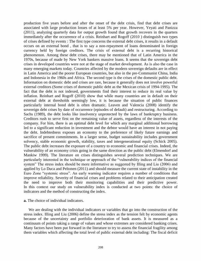
The Fig. 1 below shows that the consolidation of this situation is clearer at the end of December

2012, when bond yields in the Euro Zone fell to record lows. However, these yields are still

below market bond yields in the United States and more with those of Japan. These findings

indicates that since 2007, the bond market as also the money market has been affected by two

crises, once the American crisis, and once the crisis of the current sovereign debt, only with the

difference, it took about four years out of the first crisis (2007-2010) while it took only two years

out of the second, although it appears that the bond yields trends do not yet indicate a

stabilization. From the Fig. 2, it appears that non-financial corporations bonds recorded in 2012 a

213

yield spreads, with sovereign debt, more pronounced according to the rating is in AA, A or BBB.

The spread tightening is visible in August after new unconventional measures of the ECB.

Fig. 1 long-term government bond yields Fig. 2 corporate bond spreads of non-financial

corporations

Source: http://www.ecb.europa.eu/pub/pdf/mobu/mb201212en.pdf

3.2.2 The process of transforming data

The procedure of transforming data in variables is performed in order to have more

representative variables of financial stress. This procedure involves the following three steps: (i)

combine two data together by taking the ratio or the spread between the two. The combination of

variables has been widely used by several authors, including: Colosiez and Djelassi (1993),

Flannery and Sorescu (1996), Kaminsky and Reinhart (1999), Demirguc-Kunt and Detragiache

(1998a), Illing and Liu (2006), Lo Duca and Peltonen (2011), Hakkio and Keeton (2009), Holló

et al. (2012). But that does not prevent in certain justified cases to use data itself as a variable.

(ii) Calculate the volatility of each variable as either a simple daily variation (Holló et al. 2012;

Colosiez and Djelassi, 1993; Flannery and Sorescu, 1996; Kaminsky and Reinhart, 1999; Illing

and Liu, 2006; Lo Duca and Peltonen, 2011; Hakkio and Keeton, 2009), an absolute variation

(Holló et al. 2012) and absolute or relative absolute returns (Cajeiuro and Tobacco, 2004a,

2004b, 2008b; Holló et al. 2012; Lo Duca and Peltonen, 2011). (iii) Standardize the variables by

bringing them to a common scale by an appropriate methodology. The method most commonly

used is the variance-equal weightings. This procedure, which implicitly assumes that variables

are normally distributed, could be circumvented by standardizing variables by their Cumulative

Distribution Function (Prat-Gay and McCormick, 1999). This method is recognized by its

robustness greater than the method based on the average and the standard deviation (Stuart and

Ord, 1994).

Based on the previous three steps, we collected three variables. The selection of variables was

based on the following criteria: (i) the first criterion concern the complementarity of indicators

(Holló et al. 2012); factors need not carry the same information. (ii) The second criterion is based

on the plurality of variables; This is to take into account a number of relevant variables to

explain an episode of crisis according of the number of variables constantly evolving based on

214

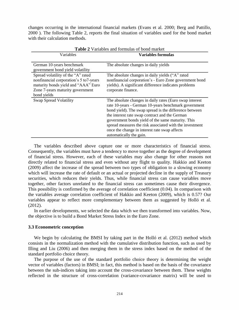
changes occurring in the international financial markets (Evans et al. 2000; Berg and Pattillo,

2000 ). The following Table 2, reports the final situation of variables used for the bond market

with their calculation methods.

Table 2 Variables and formulas of bond market

Variables Variables formulas

German 10-years benchmark

government bond yield volatility

The absolute changes in daily yields

Spread volatility of the “A” rated

nonfinancial corporation’s 5 to7-years

maturity bonds yield and “AAA” Euro

Zone 7-years maturity government

bond yields

The absolute changes in daily yields (“A” rated

nonfinancial corporation’s - Euro Zone government bond

yields). A significant difference indicates problems

corporate finance.

Swap Spread Volatility The absolute changes in daily rates (Euro swap interest

rate 10-years - German 10-years benchmark government

bond yield). The swap spread is the difference between

the interest rate swap contract and the German

government bonds yield of the same maturity. This

spread measures the risk associated with the investment

once the change in interest rate swap affects

automatically the gain.

The variables described above capture one or more characteristics of financial stress.

Consequently, the variables must have a tendency to move together as the degree of development

of financial stress. However, each of these variables may also change for other reasons not

directly related to financial stress and even without any flight to quality. Hakkio and Keeton

(2009) affect the increase of the spread between two types of obligation to a slowing economy

which will increase the rate of default or an actual or projected decline in the supply of Treasury

securities, which reduces their yields. Thus, while financial stress can cause variables move

together, other factors unrelated to the financial stress can sometimes cause their divergence.

This possibility is confirmed by the average of correlation coefficient (0.04). In comparison with

the variables average correlation coefficient of Hakkio and Keeton (2009), which is 0.57? Our

variables appear to reflect more complementary between them as suggested by Holló et al.

(2012).

In earlier developments, we selected the data which we then transformed into variables. Now,

the objective is to build a Bond Market Stress Index in the Euro Zone.

3.3 Econometric conception

We begin by calculating the BMSI by taking part in the Holló et al. (2012) method which

consists in the normalization method with the cumulative distribution function, such as used by

Illing and Liu (2006) and then merging them in the stress index based on the method of the

standard portfolio choice theory.

The purpose of the use of the standard portfolio choice theory is determining the weight

vector of variables (factors) in BMSI; in fact, this method is based on the basis of the covariance

between the sub-indices taking into account the cross-covariance between them. These weights

reflected in the structure of cross-correlation (variance-covariance matrix) will be used to

215

determine the BMSI by analogy to the optimal portfolio returns. This implies that the factors do

not all have the same weight in the BMSI.

Specifically, the calculation of the weights will be made by the solver method (an Excel feature),

which estimates the weight of each sub-index in the global index, under the condition of a

minimum variance and fixed return. To do this we use the following matrix form of the portfolio

variance of (w) securities:

(2)

: Column vector of weights, the transpose of , and

is the budget constraint and allowing holding more assets than can our initial wealth.

(3)

V: Is the variance-covariance matrix of factors.

At this level, the main methodological innovation of this BMSI compared to other composite

indicators is the application of the standard portfolio theory aggregation of factors in the BMSI,

specifically, made on the basis of weights reflecting their cross-correlation structure. As a result,

the BMSI puts relatively more weight on the situations in which stress appears in several factors

at the same time. This method differs from using the simple arithmetic average which means that

each factor has the same weight in the index (a perfect correlation between variables), which

goes against the principle of factors complementarity implies low correlation variables.

Moreover, the correlation was low and never exceeded 0.16 between the variables and 0.04 as

average which proves our complementary variables.

In what follows, the following abbreviation is used: "BMSI" indicates Bond Market Stress

Index.

3.3.1 The BMSI Graphical analysis

The evaluation criterion most widely adopted for financial stress indicators is its performance

in identifying past periods of financial stress. The reaction of an index should be evident in

response to an event causing serious turbulence in the financial system or certain losses. High

levels indicate a situation of stress or even a systemic crisis.

In our study, we take the approach of Hakkio and Keeton (2009), which is to assess whether

an index peaks are generally associated with well-known historical stress events. We develop

following episodes of stress most commonly known and which affected the financial market in

general. Figure 3 shows the following curve of the BMSI with highlighting of the most known

dates by their negative effects on the financial stability. Chosen dates correspond to events

marking the most money market in the Euro Zone during the period of our sample between

February 2007 and December 2012.

216

Fig. 3: BMSI curve

Note: Numbers 1 to 13 represent the references of dates below of events affecting more the money market

between Feb. 2007 and Dec.2012.

Table 3 Event’s references

Number Date Event

1 April 12, 2010 Exploding "subprime" in the United States.

2 May 10, 2010 BNP Paribas suspended three investment funds that have invested

in asset backed securities.

3 June 4, 2010 Collapse of Bear Stearns.

4 November 28, 2010 Bankruptcy of Lehman Brothers.

5 January 25, 2011 Abandon the U.S. plan to buy back toxic assets under the Troubled

Asset Relief Program (TARP).

6 May 17, 2011 Worsening the financial situation of Greece, Spain and Italy.

7 June 20, 2011 Waiting for a meeting September 25, 2011 the 187 member states

of the International Monetary Fund, European stock markets react

negatively.

8 July 21, 2011 Faced with the worsening debt crisis and economic indicators

turning red, economists, awards, rating agencies and analysts are

sounding the alarm.

9 October 18, 2011 Standard & Poor's threatens to lower the rating of 15 out of 17

countries, including Germany and France, before the EU summit,

European stock markets fall.

10 November 29, 2011 European shares incur losses as fears of a Greek exit from the Euro

Zone.

11 December 9, 2011 European shares fall and markets fear a failure of the EU summit.

12 December 13, 2011 Spain and Greece markets panic again.

13 March 14, 2012 European stock markets posted losses caused by the actions of

central banks on the financial sector and the cyclical situation in

Spain.

Note: Source AFP news http://www.efsf.europa.eu (economic RSS).

We note already that according to the Figure 3 shown above, the highest peaks of the Stress

Index coincide with events the more well known for their adverse effects on international

financial markets. Indeed , we report the first extreme levels from June 2007 , the date of the

global financial crisis onset, caused by the explosion of the “subprime” in the United States,

followed by suspension of BNP three investment funds that invested in asset backed securities

linked to subprime mortgage debt which had become totally illiquid on August 2007 , then we

217

still record the Bear Stearns collapse on March 2008 and the bankruptcy of Lehman Brothers on

September 2008 and finally the abandon of the U.S. plan to buy back toxic assets under the

Troubled Asset Relief Program (TARP) on November 2008. Then calm is observed, the stress

index began to fall and stock market indices resumed their upward trend. This quiet situation

continued until the beginning of 2010, when the worsening debt crisis and financial problems of

Greece are beginning to worry the rating agencies and the European stock markets. The stress

index then resume its volatility in the phenomena of successive stock market panics due to stress

accompanying the actions taken by the Euro Zone in order to appease the sovereign debt crisis

that has affected many of its countries and still persist when we conduct our research . Among

these actions we note the creation of the EFSF. This volatility extends to the last quarter of 2011,

when high levels were recorded. From this date begins a final phase of alleviation which we do

not know yet the end. This last phase is characterized by the Standard & Poor's rating agency

menaces to lower the rating of 15 out of 17 countries, including Germany and France, fears of

Greece leaving the Euro Zone, the concerns about the financial situation in Spain and Greece,

and the last event for losses caused by the measures taken by central banks and on the financial

situation in Spain and cyclical sectors. But it seems, in view of the curve, the situation tends to

improve.

3.3.2 Thresholds

One of our main goals is to build a financial stress index to help decision makers to identify

the stress levels in the Bond market which can be a serious concern. However, the identification

of truly systemic stress levels that could potentially disrupt the financial intermediation process

and economic activity is far from obvious.

In the literature several approaches are proposed to deal with this situation. One approach is

to compare the stress levels to those observed in the levels known of historical crises have caused

serious disruption. In this context, the most widely used approach is to classify financial

constraints according to their severity by exceeding the stress index of its historical average by

one or more standard deviations. For example, Illing and Liu ( 2006) for the Bank of Canada

index have used a number of 2 standard deviations ; Cardarelli et al. (2011), the IMF one

standard deviation; Hakkio and Keeton (2009), the Federal Reserve Bank of Kansas City used

also one standard deviation and Vila (2000 ) 1.5 or 2 standard deviations . A second approach

compares the index to its historical average over a moving interval of 50 days and takes only the

current stress levels exceeding this moving average by one standard deviation as a signal of

systemic risk aversion (Kantor and Caglayan, 2002).

The table 3 above chows the BMSI has reached its first peak in September 2008, reflecting

the financial difficulties unprecedented in all advanced economies and lasted longer than in any

other crisis since 1980. The second level in November 2008 confirms the high level of market

destabilization. The third level is located in May 2010 with the onset of the European sovereign

debt crisis. Finally the fourth level recorded December 2011. Among these 4 pics, the Stress

Index has exceeded its historical average of more than 1 standard deviation only in 2 events (4

and 5). We recorded also 2 events (6 and 9) with less than 1 standard deviation (see

correspondence with the events in Table 3 above and 4 below).

We classified financial constraints according to their severity by exceeding the stress index of its

historical average by 0.5 or more standard deviation in using the next formula:

(4)

218

With (NB (σ)): the standard deviations number; BMSI is the Bond Market Stress Index, E (BMSI) its mean and its standard deviation.

Table 4 BMSI discard with its historical average calculated in standard deviations numbers

Event Nr Event date Standard

deviation Nr

1 Jun-07 0,222

2 Aug-07 0,173

3 Mar-08 -0,510

4 Sep-08 2,299

5 Nov-08 1,278

6 May-10 0,875

7 Sep-10 -0,393

8 Oct-11 0,629

9 Dec-11 0,739

10 May-12 -1,079

11 Jun-12 -1,246

12 Jul-12 -1,221

13 Sep-12 -0,057

We will confirm graph N ° 1 and statistics finding (number of standard deviations) by a study

plan with Chow’s Breakpoint Test and Cusum De Brow Test. These tests are important in

understanding the course of our index which, in passage in time, the instability of coefficients in

its model reflects the events to be studied.

3.3.3 Regimes

a. Chow’s Breakpoint Test

The literature on structural changes is abundant. For example: Chow (1960), Yao (1988) and Bai

and Perron (1998). In our study we will use the Chow Test to compare if the coefficients are

identical in two or more sub-periods. The difficulty is to split the sample of observations into two

or more sub-samples (intervals). In the case of two sub-samples, a regression vectors model of

β1 and β2 parameters with the same dimension (K: number of parameters in the equation) is

adjusted. Therefore, it is to test: H0: β1 = β2 against H1: β1 ≠ β2. Chow statistic is given by:

(5)

Where SSR is the restricted sum of squared residuals under H0, SSR1 is the sum of squared

residuals from the regression of the first sub-sample. SSR2 is the sum of squared residuals from

the regression of the second sub-sample. And (T) is the total number of observations.

The use of models for structural changes results from the importance of breakpoints in chronic of

the 3 dates whether the stress index has reached its historical levels: September 2008, May 2010

and December 2011. These 3 events have been selected despite the stress index has only

exceeded its historical average by 0.5 standard due to their severity. Note that as of November

2008 is a peak stress, but we ignored the fact because it is very close to that of September 2008.

Figure 3 above is consistent with the results of the technical classification of stressful events.

Indeed, according to these two methods, we see three levels in the index. The first is in

219

September 2008, which coincides with the collapse of Lehman Brothers. The second level of

stress occurs in May 2010 triggered by the gravity of the financial situation in Greece, Spain and

Italy, as well as the beginning of the crisis of sovereign debt in the Euro Zone, the effect on the

financial stress was less important than the first period. A final highlight is spotted in December

2011 where increased stress index volatility reached a third level caused by successive panics on

the financial markets of the Euro Zone and the deepening debt crisis.

We used the Chow test to confirm the above findings emerged from Figure 3 above the

classification of stressful events based on standard deviation. Confirmations are reported in

Table 5 below.

Table 5 Chow test results

H0 H1 F-Statistic Log likelihood

ratio

Results

[Feb. 5, 2007–

Dec. 21, 2012]

[Feb. 5, 2007–Sep. 30, 2008] and

[Oct. 1, 2008–May. 10, 2010] and

[May. 11, 2010-Dec. 9, 2011] and

[Dec. 10, 2011- Dec. 21, 2012]

56.82804 ***

(0)

309.3737 ***

(0)

Break on

Oct. 1, 2008,

May. 11, 2010

and Dec. 10,

2011

[Feb. 5, 2007–

Dec. 21, 2012]

[Feb. 5, 2007– Sep. 30, 2008] and

[Oct. 1, 2008– Dec. 21, 2012] 46.72504***

(0)

90.94613***

(0)

Break on Oct.

1, 2008

[Feb. 5, 2007–

Dec. 21, 2012]

[Feb. 5, 2007–May. 10, 2010] and

[May. 11, 2010– Dec. 21, 2012]

0.304969

(0.737191)

0.611511

(0.736567)

Break on

May. 11, 2010

[Feb. 5, 2007–

Dec. 21, 2012]

[Feb. 5, 2007– Dec. 9, 2011] and

[Dec. 10, 2011– Dec. 21, 2012] 16.00363***

(0)

31.76015***

(0)

Break on

Dec. 10, 2011

Note 1: Asterisks (***, **, *) indicate the significance at (1%, 5% and 10%) of the coefficients.

Note 2: With T0 = Feb. 5, 2007; T1 = Oct. 1, 2008; T2 = May. 11, 2010; T3 = Dec. 10, 2011 and Tm+1 =

2012. With (m) is the number of breaks and (m + 1) is the number of sub-samples.

Note 3: A p-value <0.01 indicates that we reject H0, so the presence of break.

Note 4: Statistics given by Eviews 5.

Table 5 shows that p-value is equal to zero in two dates in bold (Oct. 1, 2008 and Dec. 10, 2011),

confirming only two break points. We therefore reject H0 and we are in presence of breaks on

these two dates and accept H0 in the third date (May 11, 2010). Thus, we do not admit the

assumption of stability in Oct. 1, 2008 and Dec. 10, 2011 and admit it on May 11, 2010.

b. Cusum De Brow Tests (recursive residuals)

Cusum test “Cumulative sum” is based on the cumulative sum of recursive residuals.

Recursive residuals represent the difference between the cumulative prediction (t-1) by (t) and

actual in (t). These tests are graphical tests to admit or not the assumption of stability. The

advantage of this type of testing is that it allows conducting a study of a regression stability

without defining a priori the date of break on the coefficients. The stability criterion is the

following: if the cumulative sum goes outside the area between the two critical lines is that the

coefficients are unstable. As against, if not, is that the model coefficients are stable.

By subjecting our stress index regression to this test, we confirmed the change of structure at

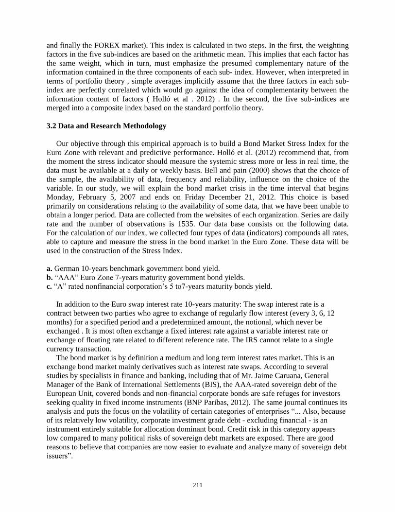
the same two dates of the Chow test. Figure 4 below shows the positioning of this curve with

respect to the range defined by the dotted lines.

220

Fig. 4 Cusum De Brow test result

The Fig. 4 shows that the curve out of the corridor in the two dates (Oct. 1, 2008 and Dec. 10,

2011) confirming the results of the Chow breakpoint test (Statistics given by Eviews 5).

Thus, all these results (graphical analysis, standard deviation, Chow and Cusum tests) confirm

the performance of our MMSI in identifying past periods of financial stress, this is proven by the

response of our index to events causing severe turbulence in the Euro Zone and by high levels

indicating a situation of stress or even a systemic crisis in times of break Oct. 1, 2008 and Dec.

10, 2011. These dates correspond to well-known events of historical stress through their effects

on financial stability during the period of our sample between Feb. 2007 and Dec. 2012. So we

confirm the ability of our BMSI to identify past periods of financial stress. In addition, we also

confirm the ability of the BMSI to help policy makers to identify stress thresholds in the

financial system that could be a real imbalance and affirm the possibility of speaking threshold to

explain the extent of financial instability.

4. Anti-crisis measures impact on the BMSI

Faced with worsening public deficits of some countries in the Euro Zone the17 members of

the Euro Zone had to implement strict policy compression expenses of its member States

affected by the crisis in order to reduce their sovereign debt, in addition to the creation of

European Financial stability Fund (EFSF), strongly bailed out by AAA member States. This

bailout is to stop definitely the contagion.

In this context, we propose a model with better predictive performance and management of

the crisis of European sovereign debt.

4.1 A summary of literature

Although the limited literature in relation to the EFSF impact on the financial stress, due to

the subject topicality, we will still present some work on the measurement of rescues actions

significance undertaken by the Euro Zone since the first fund in 2010.

Since November 2009, the debt weight has continued to increase especially for Greece. This

led the Euro Zone to intervene to avoid payment default despite the risks. The behavior of an

actor insured against the risk grows to take more risk and increases the likelihood of the risk in

question (Bastidon et al. 2012). The defaults are the result of a failure of coordination among

stakeholders of the need for a rapid response that depends on the degree of insolvency of the

State, a restructuring of a bailout and political crisis prevention.

-.5

-.4

-.3

-.2

-.1

.0

.1

.2

.3

.4

2007 2008 2009 2010 2011 2012

Recursive Residuals ± 2 S.E.

221

The restructuring of Greek sovereign debt imposes particular to ask questions and further

analysis on the effectiveness and even the usefulness of preventive measures for the management

of crises through the creation of financial rescue fund (EFSF then ESM), knowing that

management decisions does not always seem to be taken in the right direction. Indeed, (Bastidon

et al. (2012) showed that the two rate increases by the ECB in April and July 2011 have had a

destabilizing effect on bank intermediation, because they do not conform to the following

theoretical requirements which unconventional measures should primarily preserve the

commitment to maintain sustainable rates at very low levels.

In a study covering the period 2008-2011, Serbini and Huchet (2013) showed that the quality

of bank intermediation and the nature of tax efforts implemented, condition spreads versus

Germany (sovereign spreads in the Euro Zone), and that aversion is the result of a degraded

environment, including the state of public finances. These authors found that the highest spread

is that of Greece. In addition, by introducing the EFSF as a dummy variable, the authors show

that this variable is significantly positive on the spread. This variable takes into account the first

aid plan in place for Greece in May 2010 and the first payments of the EFSF to Ireland and

Portugal, respectively in February 2011 and June 2011.

Attinasi et al. (2009), in a work on measures to support the banking sector, used dummies

variables taking the value 1 the only day of the announcement of a bank bailout and take into

account the size of guarantees and recapitalizations . The dummy variable used by Barrios et al.

(2009) to capture rescues during the period following the announcements envelopes of bailouts

by national banks is not significant. Zgueb Rejichi (2011) used five dummy variables to study

the behavior of the Hurst exponent as a result of financial reforms of equity market in the MENA

region.

Hakkio and Keeton (2009), whose work has focused on well-known historical stress events,

require that financial stress index must be either efficient in identifying past periods of financial

stress “in-sample” and in future period “out-of-sample”. These authors evaluated the KCFSI

ability to predict the CFNAI comparing forecast errors of “out-of-sample” model using only

lagged values; Preliminary analysis suggests that the use of information on the KCFSI improves

“out-of-sample” CFNAI forecasts in some horizons but not others. The indicator of financial

stress must finally be effective in the identification of future periods of financial stress and

predict stressful events (Lo Duca and Peltonen, 2011; Banque de France, 2011). A performance

indicator should emit significant signals “in-sample” and “out-of-sample”. A test results of four

early warning models made before the crisis on the Asian crisis showed that the best of them was

efficient at 50 % “in-sample” (half of the crises were planned) and 33% “out-of-sample”. Berg

and Pattillo (2000) and Kaminsky & Reinhart (1999) used the ratio (noise / signal) to test the “in-

sample” performance.

In general, the prediction horizon differs depending on the cases; it can reach up to twenty-

four months in case of monthly data frequency and one to three years if they are annuals

(Kaminsky and Reinhart, 1999; Demirguc-Kunt and Detragiache, 2000). Lo Duca and Peltonen

(2011) insist on the time horizon in predicting the occurrence of systemic events. These authors

set the time horizon to 6 quarters; they justify this choice by the need to provide policy makers

with a suitable time interval in order to adopt measures to prevent the occurrence of systemic

events. The prediction horizon is a condition that must be neither short to implement a

prevention policy after the outbreak of the alert, or long for that predictions do not lose their

reliabilities (Demirguc-Kunt and Detragiache, 2000; Bussiere and Fratzscher, 2006).

In order to analyze the volatility of the stress index, we will use the methodology based on the

application of ARCH / GARCH models. To measure the effect of macroeconomic shocks on the

222

level and volatility of spreads, Arru et al. (2012) and Slingenberg and de Haan (2011) used a

GARCH methodology.

4.2 Data and Research Methodology

Our research methodology consists of four steps, primarily the study of statistical properties

of the BMSI serial. We retain this data as first data serial for our empirical investigation.

Secondly we identify the ARMA (p, q) to be used for our serial. The third stage will concern the

GARCH modeling of the process selected in the previous step. This model will serve to study the

impact of anti-crisis measures on the BMSI. Finally we close by the introduction in the selected

conditional variance model additional effects of explained variables as four dummies to measure

the impact of these four measures among eighteen taken by the European emergency fund during

the period between on May 9, 2010 (date of the EFSF creation) and the Dec. 21, 2012 end date

of our sample. We recall that these measures have been taken to rescue countries experiencing

difficulties in honoring their commitments and pay their sovereign debts. These four dates are a

second data of our study. The goal is to find a possible match between these four dates and the

decrease of the BMSI.

4.3 Empirical Results

4.3.1 Descriptive statistics

As indicated previously, our index has already been calculated, our present task is just to

check the normality and stationary. The analysis concerns the normality and stationary of the

serial distribution on the period beginning Monday, February 5, 2007 and ends Friday, December

21, 2012. The assumption of normality is verified by the Skewness and kurtosis near 0 and 3

respectively. Stationary, however, has been verified by the absence of a unit root at different

thresholds of significance and using the ADF test (1979, 1981) and the Phillips-Perron test. The

results of these tests are shown in the following Tables 6 and 7:

Table 6 Descriptive statistics of the BMSI

MMSI

Skewness -0.079446

Kurtosis 2.587963

Jarque-Bera 12.47324

Note: Statistics given by Eviews 5

Table 7 Results of the serial stationary test of MMSI

Lags

N°

Model

N°

Statistic

ADF/PP

Critical

value 1%

Critical

value 5%

Critical value

10%

Result

ADF 10 3 -6.170102 -3.964077 -3.412761 -3.128358 Stat

PP 10 3 -34.01394 -3.964037 -3.412742 -3.128346 Stat

Note 1: Column “lags N°” indicates the order of the autoregressive process used for the serial.

Column “model” indicates: Model 3 (model with constant and trend). Column “Statistic PP/ADF”

indicates statistic Dickey Fuller / Phillips-Perron. Columns “Critical value 1%”, “5%” and “10%” indicate

the critical value respectively 1%, 5% and 10% and column “Result” shows the results of the stationary

test.

Note2: Statistics given by Eviews 5

223

4.3.2 Volatility modeling

Modelling the mean volatility of the BMSI serial made clear the ARMA (1.1), ARMA (1.2)

and ARMA (2.1) which after checking the heteroscedasticity condition were subject to the

conditions of the model choice GARCH / EGARCH (p, q). After estimating the serials process

and performed tests of statistical significance of each coefficient of the selected process and the

estimation by the maximum likelihood method, we selected the ARMA (1.2)-GARCH (0.1)

model. The Table 8 below shows the process used. Among the reasons for eliminating some

models among others we can mention the probability of the test statistic ARCH-LM> 5%, the

negativity of some of their coefficients or as the non-significance of some coefficients a, α, b and

β. The detailed parameters of the selected model are given in Table 8 below:

Table 8 Estimation results by the method of maximum likelihood

Parameters Process: ARMA (1.2)-GARCH(0,1)

Mean equation

C 0.447348**

(0.0376)

a1 (AR(1)) 0.998695***

(0.0000)

a3 (MA(1)) -0.887262***

(0.0000)

a4 (MA(2)) -0.049769***

(0.0365)

Variance equation

0.000129

(0.5350)

0.992713***

(0.0000)

Q (11) 5.2783

(0.727>5%)

Q² (11) 63.877

(0.001<5%)

LM 38.41652

(0.000000<5%)

Note 1: Q (11) and Q² (11) are the statistics of Ljung-Box Q (Q-stat) the first 11 autocorrelations standard

residuals and squared residuals, LM is the Statistic of ARCH-LM test, the values in parentheses represent

probabilities t-Student and asterisks (***, **, *) indicate the significance at (1%, 5% and 10%) of the

coefficients.

Note 2: Chosen models are in bold.

Note 3: Statistics given by Eviews 5.

In reviewing the above Table 8, we note that the selected ARMA (1.2) - GARCH ( 0,1 )

model has significant mean equation parameters at 1% and β coefficient significant at 1%,

indicating the existence of ARCH effect and showing the dependence of BMSI volatility on

time. Furthermore we find that the probability of Ljung-Box statistic of the first 11 standard

residues autocorrelations is greater than 5 % indicating that future values do not depend on past

values and no significant correlation of the successive variations, whereas the probabilities of

Ljung-Box statistic of the first 11 square residues autocorrelations is less than 5 % indicating that

224

the future values depend on past values and the significant correlation of the successive

variations.

Thus, according to the test results presented above, we can assume that this model is

statistically adequate for modeling with dummies. The selected model will be used later to study

the impact of the implementation of anti-crisis measures on the BMSI.

4.3.3 Evaluation of the predictive power of the selected model (robustness checks)

After estimating the GARCH model, we will now determine whether this model provides a

better prediction based on the two prediction methods: The static and dynamic method. We used

a forecasting time horizon of 90 observations for the two methods “in-sample” and “out-of-

sample” forecast. The forecast period considered covers an “out-of-sample” forecast time

interval from Dec. 24, 2012 to April 26, 2013 and “in-sample” from Aug. 20, 2012 to Dec. 21,

2012. The following Table 9 shows the values of the standard criteria RMSE, MAE, MAPE and

TIC, obtained by sequences of 90 observations for the static and dynamic forecasting.

Table 9 Chow test result

Test Sample Static Dynamic

In-sample

forecast

[Feb. 5, 2007–Aug. 17, 2012] and

[Aug. 20, 2012–Dec. 21, 2012]

90 observations

RMSE : 0.120879

MAE : 0.099597

MAPE : 49.20438

TIC : 0.180705

RMSE : 0.142824

MAE : 0.117618

MAPE : 63.02596

TIC : 0.197230

Out-of-sample

forecast

[Feb. 5, 2007– Dec. 21, 2012] and

[Dec. 24, 2012–April 26, 2013]

90 observations

RMSE : 0.130576

MAE : 0.105589

MAPE : 26.97710

TIC : 0.121246

RMSE : 0.153106

MAE : 0.124290

MAPE : 37.17180

TIC : 0.139833

Note 1: RMSE: Root Mean Squared Error, MAE: Mean Absolute Error, MAPE: Mean Absolute Percent

Error, TIC: Theil Inequality Coefficient.

Note 2: Statistics given by Eviews 5.

From the results shown in Table 9 above, we find that using the two methods (static and

dynamic), the ARMA (1.2)-GARCH (0.1) model of the BMSI has standard criteria RMSE, MAE

and MAPE calculated according to the method of “in-sample” and “out-of-sample” very low,

indicating good predictive power forecasting. Similarly, the TIC test is very close to zero. These

findings verify the practical level performance of the BMSI in the identification of future periods

of financial stress and prediction of stressful events. We therefore use this model for modeling

BMSI with dummy variables.

4.3.4 Modelling of Stress Indices with dummies

Euro Zone, since the outbreak of the sovereign debt crisis in May 2010, has established a

number of decisions attempting to lower the high level of fiscal deficits and public debt.

Decisions include the deletion of 50% of Greek debt held by creditor banks in the country in

addition to some loans from Europe and the IMF, repetitive lowering interest rates of the major

225

Euro system refinancing operations, interest rates on the marginal lending rate, the interest rate

on the deposit facility, conducting two operations to provide liquidity in the longer term for a

period of three years, reduction in the rate of reserve requirements, the creation of the EFSF etc.

Measures taken under the EFSF during the period April 12, 2010 to December 21, 2012 (date of

the end of our sample) are showed in Table 10 below.

Table 10 Anti-crises measures

Number Date Event

1 April 12, 2010 Allocation of 110 billion € for Greece (80 billion € EAMS, 30

billion € FMI.

2 May 10, 2010 750 billion € for stability in the Euro Zone

3 June 7, 2010 Creation of the European Financial Stability Fund EFSF

(incorporated in Luxembourg under Luxembourgish law on June

7th 2010, See

http://www.consilium.europa.eu/uedocs/cms_Data/docs/pressdata/e

n/misc/114977.pdf)

4 November 28, 2010 Allocation of 85 Billion € for Ireland

5 January 25, 2011 Coming out of the EFSF program for Ireland.

6 May 17, 2011 Decision of 78 billion € for Portugal

7 June 20, 2011 Increase of the capacity of the EFSF + European Stability

Mechanism (ESM),

8 July 21, 2011 second envelop for Greece +increase of the intervention field of

EFSF/ESM

9 October 18, 2011 Increase of the envelop of the EFSF with 1000 billion €

10 November 29, 2011 Approbation of the envelop increase of the EFSF

11 December 9, 2011 The ESM will enter into force in July 2012 and the EFSF will

continue until June 2013.

12 December 13, 2011 EFSF will make his first adjudication

13 March 14, 2012 Approbation of the second program for Greece

14 March 30, 2012 The Euro-group decides to keep the EFSF and the ESM in parallel

15 April 26, 2012 EFSF organize its first action

16 May 15, 2012 EFSF organize its first action via adjudication

17 July 20, 2012 The Euro-group guaranteed assistance to the banking sector in

Spain.

18 20/07/2012 ESM inaugurated

Source : http://www.efsf.europa.eu

We will take the effective EFSF creation date (May 9, 2010) as the start of our study of anti-

crisis measures impact cited above on bond stress in the Euro Zone since this event is the turning

point in the Euro Zone politics to deal with liquidity problems of its countries member.

Our study focuses on the impact of four of the anti-crisis measures on the situation of uncertainty

and panic and hence the financial stress. The choice of these four measures among the 18 is

based on the fact that only these four measures were associated with decisions of fund

allocations to requesting countries. Other measures are not associated with bailouts of state

budgets seeking assistance decisions. We ignored the first measurement of April 12, 2010,

although it concerns financial assistance, because the event is outside our study period.

The question to which we seek an answer is: the 4 events, do they really have an impact on the

bond market stress?

226

We use a dummy variable for each of the four selected measures, which take the value 0 before

that date and 1 after. We introduce these dummy variables in the conditional variance equation of

the BMSI serial. Insofar increased Stress Index reflects an increase in uncertainty and therefore

the stress in the bond market in general of the Euro Zone, it is estimated that these dichotomous

variables, which are supposed to contribute to alleviate the situation are negatively correlated

with the stress index. In other words, if the coefficient of the dummy variable is significant and

negative it means that the measure contributes significantly to the decrease in the BMSI and thus

to improve the stress and vice versa. According to (Elmendorf and Mankiw, 1999), public debt

increases the exposure of a country to economic and financial crises and the vulnerability of an

economy crisis goes in the same direction as the public debt. Estimation process results retained

after integration of aid and assistance measures in the form of dummy variables are presented in

the following Table 11:

Table 11 Anti-crisis measures impact on the BMSI

ARMA (1.2)-GARCH (0.1) Estimation Event kind

Coefficient Probability

0.000129*** 0.0000

0.992713*** 0.0000

Dummy 1 6.15E-17*** 0.0000 750 billion € for

stability in the Euro

Zone

Dummy 2 2.29E-17** 0.0377 Allocation of 85

Billion € for Ireland

Dummy 3 -2.84E-17* 0.0650 Decision of 78 billion

€ for Portugal

Dummy 4 2.13E-17 0.1240 second envelop for

Greece +increase of

the intervention field

of FESF/ESM

Note 1: Dummies: 1 ... 4, are dummies included in the equation of the conditional variance, sorted oldest

to newest.

Note 2: Asterisks (***, **, *) indicate the significance of (1%, 5% and 10%) of the coefficients.

Note 3: The values in bold are related to significant and negative measures.

Note 4: Statistics given by Eviews 5.

Table 11 shows the impact of four events on the stress index. It emerges that two events have

a significant and positive coefficient suggesting a negative effect on stress which increases with

the arrival of these events and one event has significant coefficient at 10% reflecting a positive

and beneficial effect on stress (in bold) and one event with insignificant coefficient were found.

This finding is consistent with that of Serbini and Huchet (2013), which by introducing the EFSF

as a dummy variable, show that this variable is significantly positive on the spread (spreads

versus Germany). Another research work confirms ours that is one of Attinasi et al. (2009), in

which work on measures to support the banking sector, found that the dummy used by Barrios et

al. (2009) to capture rescues during the period following the rescues envelopes announcements

with domestic banks is not significant. The measures studied were not all the same direction or

the same magnitude on the index conditional equation volatility. We adhere to this level with the

results of Zgueb Rejichi (2011); the volatility associated with each event varies depending on the

quality and speed of transmission of information diffused. We can say that the policy of

227

assistance and support to Euro Zone countries experiencing significant fiscal deficits and require

the EFSF rescue , as financial or regulatory measures did not have all positive and significant

effect ( negative dummies ) on the bond market stress. We find here compliance with the

research results of Bastidon et al. (2012) that encourage a deeper reflection on the effectiveness

and usefulness of the European stability fund created to save the Euro Zone. These same authors

mention the risky policy of the ECB, which sometimes does not comply with the theoretical

requirements. We conclude that the chances of the European Financial Stability Facility (EFSF)

under current conditions to save the Euro Zone in the future remain unproven and possibly other

work will decide on the issue of usefulness of the EFSF or its successors, to achieve concrete and

satisfactory results.

5. Conclusion

Faced with the worsening public deficits of some countries in the Euro Zone and the threat of

spreading to other countries or regions and disability organizations in the Euro Zone to deal with

this phenomenon , policymakers saw the need for the establishment of a rigorous policy of

compression spending, more than the creation of an European Financial Stability Fund ( EFSF)

which originally should prevent the spread of the Greek crisis to other countries of the Euro Zone

, and whose budget can reach 1.000 million €. In this context, based on a recent literature, we

developed a model that allowed us to evaluate these measures. Using a research methodology,

consisting of four steps, the most important are the identification of ARMA (p, q), the GARCH

modeling and the introduction into the conditional variance of the selected model four dummies

to measure the impact of the four measures among eighteen taken by the European emergency

funds (EFSF and successors). The successful process for modeling with dummy variables is

ARMA (1.2)-GARCH (0.1) has undergone an evaluation of its predictive power based on the

two methods of static and dynamic forecasting. We used a time horizon of forecasting 90

observations for the two forecasting methods “in-sample” and “out-of-sample” and we showed

that this model offers good predictive performance. The results obtained allowed us to verify the

performance of the indicator of financial stress in the identification of future periods of monetary

stress and predict stressful events and also helped us to exclude the possibility of failure in

practice of our BMSI to predict stressful events. We then used this model for modeling stress

indices with 4 dummy variables. The results show that only one event has a beneficial impact

(negative and significant coefficients of dummies) on the stress which decreases with the arrival

of this event. However, two coefficients are significant and positive indicating that the event has

a negative effect on stress and one not significant. The policy bailout fund through anti-crisis

measures, not all had positive and significant effects on the Bond Market Stress Index.

Moreover, taking several important decisions outside the EFSF and especially after the four

events used as dummy variables could result doubts that cover the effectiveness of these funds

support. In fact, on October and November, 2011 in order to reduce the liquidity problem faced

by the Euro Zone, the Governing Council of the ECB took decisions on monetary policy. Among

these decisions, we can mention the following: the minimum level of capital “hard” of banks

(capital and retained earnings compared to loans) should be raised to 9% (were 5%), a strong

reduction of the Greece debt by the deletion of 50% (one hundred billion euros out of a country

total public debt of 350 billion Euros), loans from Europe and the IMF to Greece with 100 billion

euros at the end of 2014 ( was 109 billion Euros on July 21, 2011 ), the decrease of the main

refinancing operations interest of the Euro system to 1.25 % on November 9, 2011 then reduced

on December 14, 2011 to 1% and on July 11, 2012 to 0.75%, the lower of the interest rates on

228

the marginal lending facility to 2.00% on November 9, 2011 and on December 14, 2011 to 1.75

% then on July 11, 2012 at 1.5 %, the interest rate on the deposit facility decreased to 0.50% on

November 9, 2011and on December 14, 2011 to 0.25 % and then on July 11, 2012 to 0 %. On

2012, conducting two operations provide liquidity in the longer term for a period of three years,

expanding the list of assets eligible as collateral accepted in Euro system refinancing operation,

reducing the reserve requirements rate from 2% to 1% and the suspension of fine-tuning

operations. In the same sense, the Euro Zone has taken some more actions such as the

implementation of another mechanism which is a special fund backed by the IMF and invited

contributions from emerging countries such as China and Russia in addition of aid from Japan.

All these findings to levels of statistical results on the usefulness of sovereign funds or multiple

decisions taken in the context of European monetary policy insist that the chances of the

European Financial Stability Facility (EFSF), under current conditions, to save the Euro Zone

remain minimal. The question remains for the moment asked and may be more works will decide

on the usefulness of the EFSF or its successor to achieve concrete and satisfactory results. We

reach the thesis that invites further reflection on the effectiveness and usefulness of the European

stability fund created to save the Euro Zone.

References

Arru, D., Iacovoni D., Monteforte, L., & Pericoli, F. M. (2012), “EMU sovereign spreads

and macroeconomic news”, MPRA Papers, 37200, University Library of Munich, Germany

Attinasi, M. G., Checherita, C., & Nickel, C. (2009), “What explains the surge in euro area

sovereign spreads during the financial crisis of 2007-09?” Working Paper Series, European

Central Bank, No. 1131, December, available at:

http://www.ecb.europa.eu/pub/pdf/scpwps/ecbwp1131.pdf

Bagehot, W. (1873), “Lombard Street”, London: Kegan Paul, Ed., 1873 (1878)

Bai, j., Perron, p. (1998), “Estimating and testing linear models with multiple structural

changes”, Econometrica, journal of econometric society, Vol.66 (1), pp. 47-78

Balakrishnan, R., Danninger, S., Elekdag, S., & Tytell, I. (2009), “The Transmission of

Financial Stress from Advanced to Emerging Economies”, Emerging Markets Finance and trade,

Vol. 47(5), pp.40-68, June

Banque de France. (2011), « déséquilibres mondiaux et stabilité financière », la revue de

stabilité financière N° 15 de février 2011, avalable at http://www.banque-france.fr

Barrios, S., Iversen, P., Lewandowska, M., & Setzer, R. (2009), “Determinants of intra-

euro government bond spreads during the financial crisis”, European Economy. Economic

Papers, 388, November 2009. Brussels. Available at:

http://ec.europa.eu/economy_finance/publications/publication16255_en.pdf

Bastidon, C., Huchet, N., & Kocoglu Y. (2012), “A second dip in the euro area money

markets in 2011? Interbank risk premia and the ECB bonds and money markets policy”, Journal

of European Theoretical and Applied Studies, Vol. 1(1), pp. 11-60

Bell, J., & pain, D., (2000), “Leading indicator models of banking crises: a critical review”,

Financial stability review, pp. 113-119, December. Available at:

http://www.bankofengland.co.uk/archive/Documents/historicpubs/fsr/2000/fsr09art3.pdf

Berg, A., & Pattillo, C. (2000), "L'art difficile de prévoir les crises", FMI Washington,

Dossier Economiques, N° 22, Juillet. Available at:

http://www.imf.org/external/pubs/ft/issues/issues22/fra/issue22f.pdf

229

Blancheton, B. (2004), ''Finances publiques de la France face à la mondialisation:

Résistance, transformation et pistes de réforme'', Cahier GRES, N° 2004-13, pp. 17-22, avalable

at : http://cahiersdugres.u-bordeaux4.fr/2004/2004-13.pdf

BNP Paribas (2012), "Investment Partners", Convictions, Mars 2012, available at:

http://www.bnpparibas-ip.lu/central/press-room/perspectives.page?l=fre&p=IP_LU-NSG)

Borensztein, E., & Panizza, U., (2009), “The Costs of Sovereign Default,” IMF Staff Papers,

Palgrave Macmillan, Vol. 56(4), pp. 683-741

Boyce, J. K., & Ndikumana, L. (2001), “Is Africa a Net Creditor? New Estimate of Capital

Flight from Severely Indebted Sub-Saharan African Countries, 1970-1996”, Journal of

Development Studies, 38(2), pp. 27-56.

Bussiere, M., & Fratzscher, M. (2006), “Towards A New Early Warning System of

Financial Crises», Journal of International Money and Finance, Vol. 25(6), pp. 953-973, October

Cajeiuro, D.O., & Tabac, B.M. (2004a), “The Hurst exponent over time: testing the

assertion that emerging markets are becoming more efficient”, Physica A: Statistical Mechanics

and its Applications, Vol. 336(3-4), pp. 521-537. May

Cajeiuro, D.O., & Tabac, B.M. (2004b), “Evidence of long range dependence in Asian

equity markets: the role of liquidity and market restrictions”, Physica A: Statistical Mechanics

and its Applications, Vol. 342(3-4), pp. 656-664. November

Cajeiuro, D.O., & Tabac, B.M. (2008b), “testing for time-varying long-range dependence

in real estate equity returns”, Chaos, Solitons and Fratals, Vol. 38(1), pp. 293-307, October

Cardarelli, R., Elekdag, S., & Lall, S. (2011), “Financial stress and economic

contractions”, Journal of Financial Stability, Elsevier, Vol. 7(2), pp. 78-97, June.

Chow, g. (1960), “Tests of equality between sets of coefficients in two linear regressions”,

Econometrica, journal of econometric society, Vol. 28(3), pp. 591-605, July.

Colosiez, G., & Djelassi, M. (1993), "La redécouverte des cycles financiers", Revue

d'Economie Financière, Vol. 26(3), pp. 109-144.

De Paoli, B., Hoggarth, G., & Saporta, V., (2009), “Output Costs of Sovereign Crises:

Some Empirical Estimates,” Bank of England Working Paper No. 362, available at

http://www.bankofengland.co.uk/publications/Documents/workingpapers/wp362.pdf

Demirguc-Kunt, A., & Detragiache, E. (1998a), “The Determinants of Banking Crises in

Developing and Developed Countries”, IMF staff papers, Vol. 45(1), pp. 81-109, Mars,

Available at:

http://www.jstor.org/discover/10.2307/3867330?uid=3739176&uid=2478796217&uid=2&uid=3

&uid=60&sid=21103498823483

Demirguc-Kunt, A., & Detragiache, E., (2000), “Monitoring Banking Sector Fragility: A

Multivariate Logit Approach”, the World Bank Economic Review, Vol. 14(2), pp. 287-307.

Elmendorf, D. W., & Mankiw, N. G., (1999), “Government debt”, Handbook of

Macroeconomics, in: J. B. Taylor & M. Woodford (ed.), Handbook of Macroeconomics, edition

1, volume 1, chapter 25, pp.1615-1669 Elsevier.

European Central Bank, (2009a), “Box 1: a global Index of Financial Turbulence”

Financial Stability Review, December, pp.21-23.

Evans, O., Leone, A., Gill, M., & Hilbers, P. (2000), “Macro prudential Indicators of

Financial System Soundness”, IMF, Occasional Paper, N°192, available at:

http://www.perjacobsson.org/external/pubs/ft/op/192/OP192.pdf

Flannery, M.J., & Sorescu, S.M. (1996), “Evidence of bank market discipline in

subordinated debenture yields: 1983-1991”, the Journal of Finance, Vol. 51(4), pp. 1347-1377,

September

230

Fostel, A., & Geneakoplos, J. (2008), “Leverage Cycles and the Anxious Economy”,

American Economic Review, Vol. 98(4), pp. 1211-1244.

Furceri, D., & Zdzienicka, A., (2011), “The Real Effects of Financial Crises in the

European Transition Economies”, Economics of Transition, Vol.19 (1), pp.1-25

Gelos, G., Sahay, R., & Sandleris, G., (2011), “Sovereign Borrowing by Developing

Countries: What Determines Market Access?” Journal of International Economics, Vol. 83(2),

pp. 243-254.

Hakkio, C. S., & Keeton, W. R. (2009), “Financial Stress: What is it, how can it be

measured, and why does it matter? Federal Reserve Bank of Kansas City, Economic Review,

Second Quarter 2009, pp. 5-50.

Holló, D., Kremer, M., & Lo Duca, M. (2012), “CISS – a composite indicator of systemic

tress in the financial system”, Working paper series, N° 1426, March 2012. European Central

Bank, available at: http://www.ecb.europa.eu/pub/pdf/scpwps/ecbwp1426.pdf

Illing, M., & Liu, Y. (2006), “Measuring Financial Stress in a Developed Country: an

Application to Canada”, Journal of Financial Stability, Vol. 2(3), pp. 243-265

Kaminsky, G., & Reinhart, C. (1999), "The Twin Crises: The Causes of Banking and

Balance-of-Payments Problems." American Economic Review, Vol.89 (3), pp.473-500

Kaminsky, G., & Reinhart, C. (2000), "On crises, Contagion, and Confusion", Journal of

International Economics, Vol. 51(1), pp.145-168

Kantor, L., & Caglayan, M. O. (2002), “Using Equities to Trade FX: Introducing the

LCVI”, JP Morgan Global Foreign Exchange Research, Investment Strategies: No. 7.

Krugman, P. A. (1979), “Model of Balance-Of-Payments Crises”, Journal of Money,

Credit and Banking, Vol.11 (3), August 1979

Krugman, P. (1988), “Financing vs. forgiving a debt overhang: Some analytical notes'',

Journal of development economics, Vol.29 (2), pp. 253-268

Leaven, L., & Valencia, F. (2008), "systemic banking Crisis, a new database”, IMF

working paper, 08/224, available at: http://www.imf.org/external/pubs/ft/wp/2008/wp08224.pdf

Lindgreen et al. (1996), "Bank soundness and macroeconomic policy”, International

monetary fund

Lo Duca, M., & Peltonen, T. (2011), “Macro-Financial Vulnerabilities and Future

Financial Stress – Assessing Systemic Risks and Predicting Systemic Events”, European Central

Bank, Working Paper series N° 1311 March 2011, Available at:

http://www.ecb.europa.eu/pub/pdf/scpwps/ecbwp1311.pdf

Masson, P.R. (1998), “Contagion: Monsoonal Effects Spillovers, and Jumps between

Multiple Equilibria”, IMF Working Paper, n° WP/98/142, Washington DC, September, available

at: http://www.imf.org/external/pubs/ft/wp/wp98142.pdf

Mishkin, F. S. (1994), “Preventing Financial Crises: An International Perspective”, the

Manchester School of Economic & Social Studies, University of Manchester, vol. 62(S1), pp 1-

40, Suppl. September

Obstfeld, M. (1994), “The Logic of Currency Crises”, NBER Working Papers, n°WP4640,

1994. Available at: http://www.nber.org/papers/w4640.pdf

Ojo Kenneth, O. (1989), “Debt Capacity Model of Sub-Saharan Africa: Economic Issues

and Perspectives”, Development Policy Review, Vol. 7(4), pp. 393-412

Prat-Gay, A. & McCormick, J. (1999), “Introducing our new liquidity and credit premia

update”, J.P. Morgan Securities, Global FX and Precious Metals Research, August.

Raffinot, M. (2001), "Dette extérieure et ajustement structurel'', Universités francophones,

EDICEF/AUPELF, Paris, p11.

231

Reinhart, C. M.., & Rogoff, K. S., (2010), “Cette fois, c’est différent", Monnaie et

financement, institutions, Pearson septembre 2010.

Rose, A., (2005), “One Reason Countries Pay Their Debts: Renegotiation and International

Trade”, Journal of Development Economics, Vol. 77(1), pp. 189–206

Sachs, J., (1989), “New approaches to the Latin American debt crisis”, International

Finance Section, Dept. of Economics, Princeton University, 1989 - 50 pages

Schick, A., (2005), “Sustainable Budget Policy: Concepts and Approaches”, OECD

Journal on Budgeting, vol. 5(1), pp. 107-126.

Serbini, B., & Huchet, N. (2013) "Efforts budgétaires, intermédiation bancaire et spreads

souverains en zone euro" Version préliminaire (5 mai 2013), Université de Savoie, Université du

Sud,Toulon-Var, available at :

http://afse2013.sciencesconf.org/conference/afse2013/pages/Huchet_Serbini_Journees_de_l_AF

SE.pdf

Sinapi, C. (2010), « Crises financières et gouvernance mondiale : Intégration financière des

économies émergentes et crises d'illiquidité : une analyse en termes de fragilité financière

internationale », Sciences Humaines Combinées (en ligne), Numéro 6 - Actes du colloque inter

doctoral 2010, 10 septembre 2010. ISSN 1961 - 9936. Available at: http://revuesshs.u-

bourgogne.fr/lisit491/document.php?id=717

Slingenberg, J. W., and de Haan, J. (2011), “Forecasting Financial Stress “, DNB Working

Paper No. 292 / April 2011. Available at:

http://www.dnb.nl/en/binaries/working%20paper%20292_tcm47-253005.pdf

Stuart, A., and Ord, J. K. (1994), “Distribution Theory”, Kendall’s Advanced Theory of

Statistics, Vol. 1, 6th edition, Halsted press (Wiley, Inc), New York.

Sturzenegger, F., (2004), “Toolkit for the analysis of debt problems”, Journal of

Restructuring Finance, Vol.1 (1), pp. 201–203

Thornton, H. (1978, 1802), “An Inquiry into the Nature and Effects of the Paper Credit of

Great Britain”, E. od F.A. Hayek, Fairfield, Augustus M. Kelley Publishers, 1978 et 1802.

Vila, A. (2000), “Asset Price Crises and Banking Crises: some empirical evidence”, BIS

Conference, Papers, no 8, pp. 232-252, available at: http://www.bis.org/publ/confer08l.pdf

Yao y. c. (1988), “Estimating the number of change-points via Schwarz’ criterion”,

Statistics and Probability Letters, Vol. 6(3), pp. 181-189

Yeyati, E. L., & Panizza, U., (2011), "The elusive costs of sovereign defaults", Journal of

Development Economics, Elsevier, vol. 94(1), pp 95-105, January

Yiu, M. S., Ho, W. Y. A., & Jin, L. (2010), “A Measure of Financial Stress in Hong Kong

Financial Market – The Financial Stress Index”, Hong Kong Monetary Authority Research, Note

02/2010, March 2010. http://www.hkma.gov.hk/media/eng/publication-and-

research/research/research-notes/RN-02-2010.pdf

Zgueb, R. I. (2011), “behavior of the Hurst exponent, financial reforms and dynamic

efficiency of stock markets in the MENA region”, thesis to obtain the degree of Doctor of

Management Science, publicly defended in April 2011, Tunis Tunisia FSEG.