Exhibit 46, entered by the California Department of Fish and Gamefor the State Water Resources Control Board 1987 Water Quality/Water Rights Proceeding on the San Francisco Bay/Sacramento-SanJoaquin Delta

The Relationship Between Pollutants andStriped Bass Health as Indicated

by Variables Measuredfrom 1978 to 1985

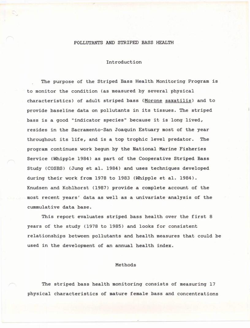
The purpose of the Striped Bass Health Monitoring Program is

to monitor the condition (as measured by several physicalcharacteristics) of adult striped bass (Morone saxatilis) and to

provide baseline data on pollutants in its tissues. The striped

bass is a good "indicator species" because it is long lived,

resides in the Sacramento-San Joaquin Estuary most of the year

throughout its life, and is ~ top trophic level predator. The

program continues work begun by the National 'Marine Fisheries

Service (Whipple 1984) as part of the Cooperative Striped Bass

Study (COSBS) (Jung et al. 1984) and uses techniques developed

during their work from 1978 to 1983 (Whipple et al. 1984).

Knudsen and Kohlhorst (1987) provide a complete account of the

most recent years' data as well as a univariate analysis of the

cummulative data base.

This report evaluates striped bass health over the first 8

years of the study (1978 to 1985) and looks for consistent

relationships between pollutants and health measures that could be

used in the development of an annual health index.

The striped bass health monitoring consists of measuring 17

physical characteristics of mature female bass and concentrations

of potential toxicants in their livers. The toxicants include

heavy metals, pesticides, and petroleum by-products (Table 1).

Liver concentrations are monitored because pollutants tend to be

concentrated by this organ as the result of its function and fat

content and yet its fat content is not high enough to interfere

with analytical procedures.

Levels of all of the variables being monitored are governed

by three factors: first, their response to each other and other

persistent features of their environment; second, "capricious"

unrelated responses of individual variables to sporadic events

that have only temporary effects; and,third, random fluctuations

in each measure. A technique known as Principal Components

Analysis (PCA) (Chatfield & Collins 1980 or Tabachnick & Fidell

1983) was used to help sort the persistent associations which

constitute "real patterns" from the sporadic responses which

amount to "noise". This technique searches for redundancy in the

data (several variables that respond in the same manner) and uses

matrix algebra and other mathematical procedures to group closely

associated variables into components. The analysis produces as

many components as there are original variables used in the data

matrix; however, individual variables may appear in more than one

component. Each sucessive component is calculated to remove the

.maximum remaining variability from the data set while still

maximizing the variance of the total component scores. The latter

causes each component to be unique and independent. The variablesmost strongly correlated with each component are those that best

TaoLE 1VARIABLES USED IN THE PRINCIPAL COMPONENT ANALYSES OF POLLUTANT & HEALTH VARIABLES FROM MATURE, FEMALE STRIPED BASS

COLLECTED IN THE SACRAMENTO - SAN JOAQUIN DELTA.

TAPERAFl'TAPELESN

EGGSTAGEPERC_RES

Cd Cr CuHCJ Zn Se

O=San Joaquin Riverl=Sacramento River

Total sum of six sections on one side of thef~sh for l=solid & 2=broken stripinCJ pattern.The sum of these scores ranCJed from 6 to 12.ECICJcolor ranCJed from yellow to CJreen scoredB to 16.Tapeworm larvae abundance ranked from1 to 5 at each location of occurrance. Thevariable is the sum of all occurances.2=few, 3=averaCJe, 4=many, 5=very many/heavilyparasitized.

Tapeworm induced lesions, scored 2-5 likeTAPELARV.

All parasites combined, scored 2-5 likeTAPELARV.Mesenteric fat abundance rank 1 to 4 where:l=none, 2=sparse, 3=averaCJe, 4=abundant.

Monocyclic aromatic hydrocarbons in liver,ppm wet weiCJht.

Transformation in PCA on:All B Yrs 1984-85

Not Used1/

Not Used1/

Arcsine-square rootNot Available!/

Relative DeCJrt,of Normality-

LOCJe Non-normalLOCJe Non-normal

LOCJe Non-normalNot UsedJ/ ApprOXimately normal

Arcsine- Non-normalsquare rootRaw, square Normal or approximately normalroot, orlOCJeasneeaed

Not used Non-normalbecause allvalues = 0

Transformation in PCA on:All 8 Yrs 1984-85

Re 1ative Degree,of Normali ty !..

Arcsine- Approximately normalsquare root

TOT_PCB Total concentration of all forms ofPCB in liver, ppm wet weight.

DDT_METa/ The summed concentration of DDT and itsmetabolic products in liver, ppb wetweight.

PESTICIn2/ The summed concentrations of allpesticides in liver, ppb wet weight.

TOT_ABN Sum of all skeletal abnormalitiesranked in severity from 1 (leastsevere) to 5 (most severe) at eachlocation of occurrence.Weight/(fork 1ength)3, a standardcondition factor for fish.

Index of fecundity = eggs perfish/weight of the fish.

None None Normal

Square root None Normal or approximately normal

Square root None Normal

None None Approximately normal or normal

Arcsine- Arcsine- Approximately normal or normalsquare root square root

None Not Used Non-normal

None None Normal

Body depth behind the operculumdivided by fork length.

Gonadosomatic index = gonad weight/fish weight.Liver somatic index = liver weight/fish weight.Days since June 1, 1960 a lineartime scale over years.Julian day of the year, representingseasonal time trends

1/ Relative degree of normality of the raw variable or after the necessary transformation indicated in the two columns atleft.

A/ Inconsistently scored over the course of the study.1/ Redundant with the individual parasite severities used in the 1984/85 analysis.1/ Not measured in the majority of fish collected between 1978 and 1983.5/ Includes p,p' -DDT; o.p-, p,p'-DDD; and o,p-, p,p' -DDE.~/ Includes toxaphene, chlordane, nonach1or, oxych1ordane, hexach1orobenzene.

describe it and reflect the most consistent relationships left in

the data matrix.Two issues need to be considered in interpreting the results

of PCA: 1) The proportion of the variability in the data matrix

explained by each component, represented by its eigenvalue.Components with eigenvalues less than one are usually ignoredsince they account for less variability in the original data than

a single variable. In essence, the object of PCA is to produce a

few components that explain most of the variation in the data and

certainly more than single variables. Catell's Scree test and an

examination of the sorted and shaded correlation matrix are

procedures often used to make an even more conservative selection

of useful components from those with eigenvalues greater than one.

For an explanation of the theory behind these last two techniques

and their method of application, see the appendix. 2) The amount

of correlation between variables and the most important

components. High correlations suggest that a component has

adequately reflected persistent associations among the original

variables. However, as in any correlation analyses, reasonable

explanations for these correlations must exist before a true

association (real pattern) is implied. Conversely, high

correlations between variables and components with low eigenvalues

(components that account for little of the variation in the

original data) do not warrant strong conclusions and may only

suggest hypotheses for future testing.

The Principal Components Analysis, over 8 years of data and

using 17 variables, exhibited only one strong component. It

reflected the sexual maturity of the fish and was unrelated to any

pollutant parameters. Hence, no component was strong enough to

provide conclusions about the relationship between striped bass

health and pollutants. However, seven components each had

eigenvalues greater than one and explained more than 5% of the

total variance in the data matrix (Table 2). Catell's Scree Test

(Figure 1) indicated that three or four of these seven components

were important, but the sorted and shaded correlation matrix

(Figure 2) indicated that, at most, two strong components existed.

The first component (Table 3) - - the one reflecting sexual

maturity - - was highly correlated with the relative size of the

ovaries (GSI) and an index of fecundity (IFECUND). A positive,although moderate, association with the variable EGGSTAGE

indicates that fishes with greater fecundity and larger ovarieshad more mature egg stages. There also is a moderate negative

association with the relative size of the liver (LSI) which may

represent a normal reduction in the proportional mass of the liver

as the fish nears spawning. A negative correlation with thepercent of eggs undergoing resorption (PERC_RES) indicates that

there is less egg resorption in mature ovaries.

TABLE 2EIGENVALUES AND PROPORTION OF VARIANCE ASSOCIATED WITH THE UNROTATED COMPONENTS FROM THE PRINCIPALCOMPONENTS ANALYSIS ON POLLUTANT & HEALTH VARIABLES FROM MATURE. FEMALE STRIPED BASS COLLECTED IN

THE SACRAMENTO - SAN JOAQUIN DELTA FROM 1978 TO 1985. (N=199)COMPONENT EIGENVALUE CUMULATIVE PROPORTION OF VARIANCE ABSOLUTE PROPORTION OF VARIANCE

it IN DATA SPACE IN COMPONENT SPACE IN DATA SPACE IN COMPONENT SPACE------ --------- ----------------------------------- ------------------------------------

1 2.9432 0.1731 0.2615 0.1731 0.26152' 1.9305 0.2867 0.4330 0.1136 0.17153 1.5701 0.3790 0.5724 0.0923 0.1394-4 1.3411 0.4579 0.6916 0.0789 0.11925 1.2170 0.5295' 0.7997 0.0716 0.10816 1.1576 0.5976 0.9025 0.0681 0.10287 1.0975 0.6622 1.0000 0.0646 0.09758 0.8981 0.7150 0.05289 0.8466 0.7648 0.0498

10 0.7681 0.8100 0.045211 0.6997 0.8511 0.041112 0.6585 0.8899 0.038813 ' 0.5846 0.9243 0.034414 : 0.4720 0.9520 0.0277 ' ,15 : 0.3776 0.9742 0.022216 0.2777 0.9906 0.016417 0.1603 1.0000 0.0094

THE EIGENVALUES ARE FOR EACH COMPONENT BEFORE ROTATION. THE CUMULATIVE OR ABSOLUTE PROPORTION OFVARIANCE IN DATA SPACE IS THE AMOUNT OF VARIABILITY IN THE ORIGINAL DATA ACCOUNTED FOR BY THATMANY COMPONENETS OR THAT COMPONENT. RESPECTIVELY. AND THE PROPORTION IN COMPONENT SPACE IS THEAMOUNT OF VARIABILITY IN THE PRINCIPAL COMPONENT ANALYSIS SOLUTION ACCOUNTED FOR BY THAT MANYCOMPONENTS (CUMULATIVE), OR THAT COMPONENT INDIVIDUALLY (ABSOLUTE).

820 " .-w·180

Z 16 ALL EZGHT YEARScT . (1978 to 19B!5)

140: i2. <~

> 10lL. 80 6X 4

20 10 12 140 2 6 B 16 18

COMPONENT M

25W0 -~984 ac ~985Z 20H

·IL 15<I:>LL 100

~ 5

o o

FIGURE l--CATELL'S SCREE TEST PLOTS OF THE PERCENT OF VARIANCE IN THE RAWDATA ACCOUNTED FOR BY EACH UNROTATED COMPONENT. COMPONENTSAREFROM ANALYSES ON POLLUTANT AND HEALTH VARIABLES IN MATURE, FEMALESTRIPED BASS FROM THE SACRAMENTO-SAN JOAQUIN DELTA. . THEAPPROPRIATE NUMBER OF COMPONENTSTO INTERPRET IS LESS THAN OREQUAL TO THE COMPONENTNUMBER AT WHICH THE CURVE BEGINS ANAPPROXIMATELY LINEAR DECLINE (1978-1985: COMPONENT#4; 1984-1985:COMPONENT #5). BELOW THAT POINT, EACH ADDITIONAL COMPONENT SIMPLYACCOUNTS FOR SIMILAR BUT GRADUALLY DECREASING PROPORTIONS OF THETOTAL VARIANCE REMAINING IN THE DATA.

61 GSI B~ 160 IFECUND ~59 BODYFROP B58 KFL . +B64 DAY_IN_Y - .. K~ 262 LSI H- -KR~2 LOCATION .... K25 EGGSTAGE B. --B-B63 TIME X X ...B36 AH +K44 TOT_PAR ..B

9 AGE +.. -K45 TOT_ABN .-B14STRPtot ..B35 MAH .. B18 RANK2EC l!28 PERC_RES XX ..X.+X.+ ..-.J!

THE ABSOLUTE VALUES OFTHE MATRIX ENTRIES HAVE BEEN PRINTED ABOVEACCORDING TO THE FOLLOWING SCHEME

LESS THAN OR EQUAL TO0.080 TO AND INCLUDING0.161 TO AND INCLUDING

+ 0.241 TO AND INCLUDINGX 0.321 TO AND INCLUDINGK 0.402 TO AND INCLUDINGB 0.482 TO AND INCLUDINGII GREATER THAN

IN SHADED FORM0.0800.1610.2410.3210.4020.4820.5620.562

FIGURE 2.-- SORTED AND SHADED MATRIX REPRESENTING CORRELATIONS BETWEEN POLLUTANTAND HEALTH VARIABLES MEASURED IN MATURE, FEMALE STRIPED BASS FROMTHE SACRAMENTO - SAN JOAQUIN DELTA, 1978 - 1985. THIS MATRIX PROVIDESA MEANS OF CONFIRMING THAT THE COMPONENTS CALCULATED BY PCA REPRESENTREAL ASSOCIATIONS BETWEEN VARIABLES. THE HEAVILY SHADED SQUARES SHOWWHICH VARIABLES ARE MOST HIGHLY CORRELATED WITH EACH OTHER. THEHIGHLY CORRELATED VARIABLES TEND TO BE THE SAME AS THOSE COMBINEDINTO THE STRONGEST COMPONENTS BY PCA, AND ARE DELINEATED BY THENUMBERED BRACKETS AT THE RIGHT EDGE OF THE FIGURE. THE LAST SQUARE INEACH ROW IS ALWAYS THE DARKEST SYMBOL AS IT REPRESENTS A CORRELATIONOF 1.0 (CORRELATION BETWEEN VARIABLE LISTED AT START OF ROW ANDITSELF). PROCEEDING ACROSS ANY ROW, THE FIRST SYMBOL INDICATES THECORRELATION OF THAT VARIABLE WITH THE FIRST VARIABLE IN THE LIST, THESECOND SYMBOL REPRESENTS ITS CORRELATION WITH THE SECOND VARIABLE INTHE LIST, ETC. SEE THE APPENDIX FOR A COMPLETE EXPLANATION.

TABLE 3SORTED ROTATED COMPONENT LOADINGS CPATl'ERN MATRIX) FOR THE PRINCIPAL COMPONENTS ANALYSIS ON POLLUTANT & HEALTH VARIABLES FROM

MATURE, FEMALE STRIPED BASS COLLECTED IN THE SACRAMENTO - SAN JOAQUIN DELTA FROM 1978 TO 1985. CN=199)COMPONENT # 1 2 3 4 5 6 7---------------------------------------------------------------------------------------------------------COMPONENT NAME SEXUAL MORPHOLOGY & SACRAMENTO LESS ALYCYCLIC OLDER FISH ABNORMALITIES & MONOCYCLIC

MATURITY SEASONAL LIVER RIVER FISH HEXANES THROUGH WITH MORE BROKEN STRIPING AROMATICCONDITION TIME PARASITES PATrERN HYDROCARBONS

GSI 0.860 0.000 0.000 0.000 0.000 0.000 0.000IFECUND 0.849 0.000 0.000 0.000 0.000 0.000 0.000BODYPROP 0.000 0.635 0.000 0.000 0.000 0.000 0.000KFL 0.000 0.625 0.000 -0.418 0.000 0.318 0.000DA'CIN_Y 0.000 -0.539 0.000 0.000 0.000 0.000 0.000LSI -0.404 0.520 0.416 0.000 0.000 0.000 0.000LOCATION 0.000 0.000 0.753 0.000 0.000 0.000 0.000EGGSTAGE 0.433 0.000 -0.664 0.000 0.000 0.000 0.000TIME 0.000 0.000 0.000 0.769 0.000 0.000 0.000AH 0.000 0.000 0.000 -0.696 0.000 0.000 0.000TOT_PAR 0.000 0.000 0.000 0.000 0.764 0.000 0.000

I-'AGE 0.000 0.000 0.000 0.000 0.682 0.000 0.000 0TOT ABN 0.000 0.000 0.000 0.000 0.000 0.792 0.000STRPtot 0.000 0.000 0.000 0.000 0.000 0.581 -0.447HAM 0.000 0.000 0.000 0.000 0.000 0.000 0.781RANK2EC 0.000· -0.487 0.000 0.000 0.000 0.000 0.000PERC_RES -0.475 0.000 0.000 -0.334- 0.000 0.000 0.444-

% OF VARIANCE 13.52 9.87 9.45 9.41 8.l4 7.94 7.88THE ABOVE COMPONENT LOADING MATRIX HAS BEEN REARRANGED SO THAT THE COLUMNS APPEAR IN DECREASING ORDER OF VARIANCE EXPLAINED BYCOMPONENTS. THE ROWS HAVE BEEN REARRANGED SO THAT FOR EACH SUCCESSIVE COMPONENT. LOADINGS GREATER THAN 0.5000 APPEAR FIRST.LOADINGS LESS THAN 0.3160 HAVE BEEN REPLACED BY ZERO AS THEY WERE NOT INTERPRETED. THE "% OF VARIANCE" EQUALS THE AMOUNT OFVARIABILTY CVARIANCE) IN THE ORIGINAL DATA ACCOUNTED FOR BY THAT SPECIFIC COMPONENT. A "NAME" WAS ASSIGNED TO EACH COMPONENTBASED ON THE VARIABLES THAT WERE MOST HIGHLY CORRELATED WITH IT, TO HELP THE READER INTERPRET AND IDENTIFY INDIVIDUAL COMPONENTS.

The remaining six components each explain less than 10% of

the variance in the data matrix (Table 3), are highly correlated

with only a few variables, and are derived from at most one strong

and a few weak bivariate correlations. For these reasons, any

associations between pollutants and striped bass health exhibited

by these components must, at best, be considered as no more than

working hypotheses.

Five intermediately correlated variables representing

body proportion, condition factor, time in days into the spawning

season, relative liver size, and egg color (BODYPROP, KFL,

DAY_IN_Y, LSI, RANK2EL) make up the second component (Table 3).

However, an examination of the sorted and shaded correlation

matrix (Figure 2) and the bivariate correlation matrix (Table 4)

indicates that body proportion (BODYPROP) and condition factor

(KFL) are not very well related to the others. The two

associations between 1) deep body proportion and condition factor

(Table 3 and 4), and 2) proportional liver size (LSI), which tendsto be greater early in the season, and yellowish egg color (low

RANK2EC), which is an indication of immature eggs, are logical

redundancies and provide no indication of the relationship between

pollutants and fish health.

The third component, like the first, reflects the

relationship between larger proportional liver size (LSI) and a

less mature dominant eggstage in the ovary (EGGSTAGE) and also

indicates that sampling in the Sacramento River tended to collectfish with earlier egg stages.

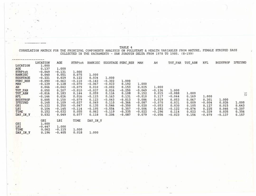
·.. -------- .----TABLE 4

CORRELATION MATRIX FOR THE PRINCIPAL COMPONENTS ANALYSIS ON POLLUTANT & HEALTH VARIABLES FROM MATURE. FEMALE STRIPED BASSCOLLECTED IN THE SACRAMENTO - SAN JOAQUIN DELTA FROM 1978 TO 1985. (N=199)

------------------LOCATION AGE STRPtot RANK2EC EGGSTAGE PERC_RES MAli AH TOT_PAR TOT_ABN KFL BODYPROP IFECUND

LOCATION 1.000AGE 0.137 1.000STRPtot -0.049 -0.131 1.000. RANK2EC 0.040 0.051 0.075 1.000EGGSTAGE -0.221 0.029 0.122 0.034 1.000PERC_RES -0.090 -0.062 -0.110 -0.142 -0.302 1.000MAli -0.129 0.128 -0.070 -0.067 -0.023 0.192 1.000AH 0.046 -0.042 -0.079 0.010 -0.002 0.153 0.025 1.000TOT_PAR 0.050 0.207 -0.010 -0.037 0.016 -0.250 -0.049 -0.136 1.000TOT_ABN -0.016 0.183 0.144 0.059 0.116 0.108 0.152 0.015 -0.088 1.000 •....KFL -0.146 0.026 0.016 -0.115 0.163 0.131 -0.010 0.117 -0.044 0.169 1.000 N

BODYPROP 0.005 0.150 -0.079 0.123 -0.043 -0.013 0.086 0.029 0.053 0.067 0.301 1.000IFECUND 0.148 0.109 -0.037 0.049 0.110 -0.366 -0.087 -0.070 0.031 0.009 -0.004 0.026 1.000GSI -0.122 0.250 -0.047 0.135 0.546 -0.350 0.020 -0.053 0.030 0.105 0.127 0.015 0.643LSI 0.104 -0.145 -0.114 -0.195 -0.554 0.357 -0.006 0.082 -0.122 -0.074 0.225 0.046 -0.207TIME 0.152 -0.032 0.055 0.062 -0.119 -0.335 -0.022 -0.296 0.114 0.022 -0.339 0.035 0.356DAY_IN_Y 0.032 0.049 0.077 0.118 0.206 -0.087 0.079 -0.056 -0.023 0.156 -0.079 -0.137 0.157

GSI LSI TIME DAY_IN_YGSI .1.000LSI -0.447 1.000TIME 0.062 -0.115 1.000DAY_IN_Y 0.196 -0.405 0.018 1.000

Components 4 and 7, respectively, show associations between

alicyclic hexanes or monocyclic aromatic hydrocarbons and

increased egg resorption. However, because the correlations among

the individual variables are so small (Table 4) and the components

account for such a small proportion of the total variability inthe data (Table 3), a conclusion that the accumulation of these

compounds in fish affects resorption is not warranted. These

results only point to hypotheses for future testing.

The fifth component shows an increase in total parasites with

the age of the fish, but doesn't associate this increase with any

pollutant variables.

Component number six indicates that the total number of·

skeletal abnormalities, composed mostly of abnormalities in the

gill rakers, is associated with fishes having a more broken

striping pattern and that there is a slight positive relationship

between more robust fish (large KFL) and skeletal abnormalities.

There is no indication of pollutant effects.

In the most recent 2 years of the health monitoring, many

more pollutant variables were measured in all fish sampled than

in the first 6 years. Hence, the more recent data yield more

insight about the relationship between pollution and fish health.

Of course, the conclusions drawn from these 2 years of data

reflect only what happened in 1984 and 1985. It remains to be

seen whether the 1986 and 1987 data, which we have collected and

are processing, support these trends.

Eight components were interpretable and had eigenvalues

greater than one (Table 5) and each explained more than 5% of the

total variance after rotation (Table 6). According to Catell's

Scree Test (Figure 1), the first four or five components should beinterpreted and an inspection of the sorted and shaded correlation

matrix confirmed that, at most, there were five strong components

(Figure 3). The first five components had three or more

correlations with the original variables that were greater than

0.50 (Table 6). Three of the first five components demonstrated

some degree of pollutant-fish health relationsips. The sixth,

seventh, and eighth components represented very weak relationships

that also are presented here simply as potential working

hypotheses.

As in the analysis based on all 8 years, the first component

(Table 6) is a sexual maturity component, and again, there is no

evidence of pathological problems caused by pollutants despite

associations with zinc, copper, cadmium and selenium in the liver.Percent egg resorption is now positively associated with sexual

maturity rather than negatively as in the analysis over 8 years,

but the relationship is still weak. There is a slight tendency

for a decrease in percent lipid in the liver with increasing

maturity of the ovaries. Variables representing increasing sexual

maturity are also slightly associated with collections made later

in the season. The second component (Table 6) represents a

relationship between pesticides, DDT and its metabolites, total

TABLE 5EIGENVALUES AND PROPORTION OF VARIANCE ASSOCIATED WITH THE UNROTATED COMPONENTS FROM THE PRINCIPAL

COMPONENTS ANALYSIS ON POLLUTANT & HEALTH VARIABLES FROM MATURE. FEMALE STRIPED BASS COLLECTED INTHE SACRAMENTO - SAN JOAQUIN DELTA IN 1984 & 1985. (N=74)

COMPONENT EIGENVALUE CUMULATIVE PROPORTION OF VARIANCE ABSOLUTE PROPORTION OF VARIANCE• IN DATA SPACE IN COMPONENT SPACE IN DATA SPACE IN COMPONENT SPACE------ --------- ----------------------------------- ------------------------------------

1 6.8108 0.2349 0.3309 0.2349 0.3309'l 2.8981 0.3348 0.4716 0.0999 0.1407.;.3 2.7935 0.4311 0.6073 0.0963 0.13574 2.3164 0.5110 0.7199 0.0799 0.11265 1.6768 0.5688 0.8013 0.0578 0.08146 1.5009 0.6206 0.8742 0.0518 0.07297 1.3681 0.6677 . 0.9407 0.0471 0.06658 1.2208 0.7098 1.0000 0.0421 0.05939 1.0591 0.7464 0.0366

10 0.9937 0.7806 0.034211 0.8161 0.8088 0.028212 0.7763 0.8355 0.026713 0.5948 0.8561 0.0206 ....14- 0.5741 0.8759 0.0198 lJ1

15 0.5262 0.8940 0.018116 0.4341 0.9090 0.015017 0.3802 0.9221 0.013118 0.3702 0.9348 0.012719 0.3174 0.9458 0.011020 0.2994 0.9561 0.010321 0.2808 0.9658 0.009722 0.2146 0.9732 0.007423 0.1948 0.9799 0.006724 0.1540 0.9852 0.005325 0.1479 0.9903 0.005126 0.1196 0.9944 0.004127 0.0861 0.9974 0.003028 0.0475 0.9990 0.0016.29 0.0276 1.0000 0.0010

THE EIGENVALUES ARE FOR EACH COMPONENT BEFORE ROTATION. THE CUMULATIVE OR ABSOLUTE PROPORTION OFVARIANCE IN DATA SPACE IS THE AMOUNT OF VARIABILITY IN THE ORIGINAL DATA ACCOUNTED FOR BY THATMANY COMPONENETS OR THAT COMPONENT. RESPECTIVELY, AND THE PROPORTION IN COMPONENT SPACE IS THEAMOUNT OF VARIABILITY IN THE PRINCIPAL COMPONENT ANALYSIS SOLUTION ACCOUNTED FOR BY THAT MANYCOMPONENTS (CUMULATIVE), OR THAT COMPONENT INDIVIDUALLY (ABSOLUTE).

TABLE 6SORTED ROTATED COl1PONENT LOADINGS (PATTERN MATRIX) FOR THE PRINCIPAL COr1PONENTS ANALYSIS ON POLLUTANT & HEALTH VARIABLES FROM

MATURE. FEMALE STRIPED BASS COLLECTED IN THE SACRAMENTO - SAN JOAQUIN DELTA IN 1984 & 1985. (N=741COMPONENT # 1 2 3 4 5 6 7 8--------------------------------------------------------------------------------------------------------COMPONENT NAME SEXUAL FAT SOLUBLE PARASITES & MORPHOLOGY. LEAN OLDER FECUNDITY & TAPEWORM YELLOWMATURITY POLLUTANTS TRACE METALS SEASON & Cr FISH & Hg FISH LESIONS & EGG COLORCONDITION RAFTS & MAW s

EGGSTAGE 0.857 0.000 0.000 0.000 0.000 0.000 0.000 0.000LSI -0.806 0.000 0.000 0.000 0.000 0.000 0.000 0.000Zn 0.742 0.000 0.000 0.000 0.000 0.000 0.000 0.000Cu 0.685 0.000 0.000 0.000 0.000 0.000 0.000 0.418GSI 0.638 0.000 0.000 0.000 0.000 0.540 0.000 0.000PESTICID 0.000 0.854 0.000 0.000 0.000 0.000 0.000 0.000DOT_MET 0.000 0.842 0.000 0.000 0.000 0.000 0.000 0.000LIPID -0.399 0.707 0.000 0.358 0.000 0.000 0.000 0.000TOT PCB 0.000 0.688 0.000 -0.351 0.000 0.000 0.000 0.000TAPELARV 0.000 0.000 0.765 0.000 0.000 0.000 0.000 0.000Cd 0.455 0.000 0.623 0.000 0.000 0.000 0.000 0.000RNDWLARV 0.000 0.000 0.592 0.000 0.000 0.000 0.000 0.000Se 0.383 0.000 0.544 0.000 0.347 0.000 0.000 0.371BODYPROP 0.000 0.000 0.000 0.872 0.000 0.000 0.000 0.000Cr 0.000 0.000 0.000 -0.678 0.000 0.000 0.000 0.000 r-'

0\DAY IN Y 0.354 0.000 0.000 -0.613 . O.000 0.000 0.000 0.000MES:FAT 0.000 0.322 0.000 0.000 -0.740 0.000 0.000 0.000Hq 0.000 0.000 0.000 0.000 0.723 0.000 0.000 0.000AGE 0.000 0.000 0.497 0.000 0.574 0.000 0.000 0.000IFECUND 0.000 0.000 0.000 0.000 0.000 0.810 0.000 0.000KFL 0.000 0.000 -0.430 0.000 -0.356 0.573 0.000 0.000TAPELESN 0.000 . 0.000 0.000 0.000 0.000 0.000 0.788 0.000TAPERAFT 0.000 0.000 0.000 0.000 0.000 0.000 0.744 0.000RANK2EC 0.000 0.000 0.000 -0.370 0.000 0.000 0.000 -0.704MAH 0.000 0.000 0.000 0.000 0.000 0.000 0.000 0.689STRPtot 0.000 0.000 0.000 0.000 0.413 0.000 0.359 0.000PERC_RES 0.429 0.319 0.000 0.000 0.000 -0.462 0.000 0.000LOCATION 0.000 0.429 0.449 0.000 0.000 0.000 -0.349 0.000TOT_ABN 0.354 0.000 0.000 0.000 0.000 0.000 0.000 0.000

% OF VARIANCE 14.14 11. 86 9.73 8.18 7.99 6.62 6.40 6.06THE ABOVE COr1PONENT LOADING MATRIX HAS BEEN REARRANGED SO THAT THE COLUMNS APPEAR IN DECREASING ORDER OF VARIANCE EXPLAINED BYCOMPONENTS. THE ROWS HAVE BEEN REARRANGED SO THAT FOR EACH SUCCESSIVE COMPONENT. LOADINGS GREATER THAN 0.5000 APPEAR FIRST.LOADINGS LESS THAN 0.3160 HAVE BEEN REPLACED BY ZERO AS THEY WERE NOT INTERPRETED. THE "% OF VARIANCE" EQUALS TP.E AMOUNT OFVARIABILTY (VARIANCE) IN THE ORIGINAL DATA ACCOUNTED FOR BY THAT SPECIFIC COMPONENT. A "NAME" WAS ASSIGNED TO EACH COr1PONENTBASED ON THE VARIABLES THAT WERE MOST HIGHLY CORRELATED WITH IT. TO HELP THE READER INTERPRET AND IDENTIFY INDIVIDUAL COMPONENTS.

25 EGGSTAGE II~i2 LSI BII 133 Zn HHII31 Cu XXXII61 GSI HXX+II43 PESTICID -X+-~242 DDT_MET -++-+BK38 LIPID +HX-XBBII39 TOT_PCB .- •• X++II ~21 TAPELARV • --. -+- II 329 Cd -X+X+XX+ HII23 RNDWLARV. .- ••• --1134 Se -+XH+XXX XB-II59 BODYFROP -+. 0 430 Cr .- •.•• + ~~64 DAY_IN_Y ++1124 MES· FAT --- -++X.. • 1I~532 Hg - .--.XX+X .-+X •• XII

9 AGE • -+- •• -XII60 IFECUND X... ..--1158 KFL ••• -.1146 TAPELESN • • •• •• II22 TAPERAFT -+. • +1118 RANK2EC •• -+-. II35 MAH • +1114 STRPtot •• II28 PERC_RES -. • ••• • ••• 11

2 LOCATION - - +. II5 TOT_ABN • •• • • • • • • • • II

THE ABSOLUTE VALUES OFTHE MATRIX ENTRIES HAVE BEEN PRINTED ABOVE IN SHADED FORMACCORDING TO THE FOLLOWING SCHEME

LESS THAN OR EQUAL TO0.115 TO AND INCLUDING0.230 TO AND INCLUDING0.345 TO AND INCLUDING0.460 TO AND INCLUDING0.575 TO AND INCLUDING0.690 TO AND INCLUDING

GREATER THAN

0.1150.2300.3450.4600.5750.6900.8050.805

FIGURE 3. -- SORTED AND SHADED MATRIX REPRESENTING CORRELATIONS BETWEEN POLLUTANTAND HEALTH VARIABLES MEASURED IN MATURE, FEMALE STRIPED BASS FROMTHE SACRAMENTO- SAN JOAQUIN DELTA, 1984 - 1985. THIS MATRIX PROVIDESA MEANS OF CONFIRMING THAT THE COMPONENTSCALCULATED BY PCA REPRESENTREAL ASSOCIATIONS BETWEEN VARIABLES. THE HEAVILY SHADED SQUARES SHOWWHICH VARIABLES ARE MOST HIGHLY CORRELATED WITH EACH OTHER. THEHIGHLY CORRELATED VARIABLES TEND TO BE THE SAME AS THOSE COMBINEDINTO THE STRONGEST COMPONENTSBY PCA, AND ARE DELINEATED BY THENUMBEREDBRACKETS AT THE RIGHT EOOE OF THE FIGURE. THE LAST SQUARE INEACH ROW IS ALWAYSTHE DARKEST SYMBOLAS IT REPRESENTS A CORRELATIONOF 1.0 (CORRELATION BETWEEN VARIABLE L:J:STED AT START OF ROWANDITSELF). PROCEEDING ACROSS ANY ROW, THE FIRST SYMBOL INDICATES THECORRELATION OF THAT VARIABLE WITH THE FIRST VARIABLE IN THE LIST, THESECOND SYMBOL REPRESENTS ITS CORRELATION WITH THE SECOND VARIABLE INTHE LIST, ETC. SEE THE APPENDIX FOR A COMPLETE EXPLANATION.

logical as all of these toxicants are fat soluble. The

correlations also suggested that these pollutants are weakly

Component number four indicates that fish with a deeper body

form (BODYPROP) have lower concentrations of chromium in their

these traits also tended to have slightly more lipid in the liver,

slightly lower total PCBs, and slightly more yellowish or immature

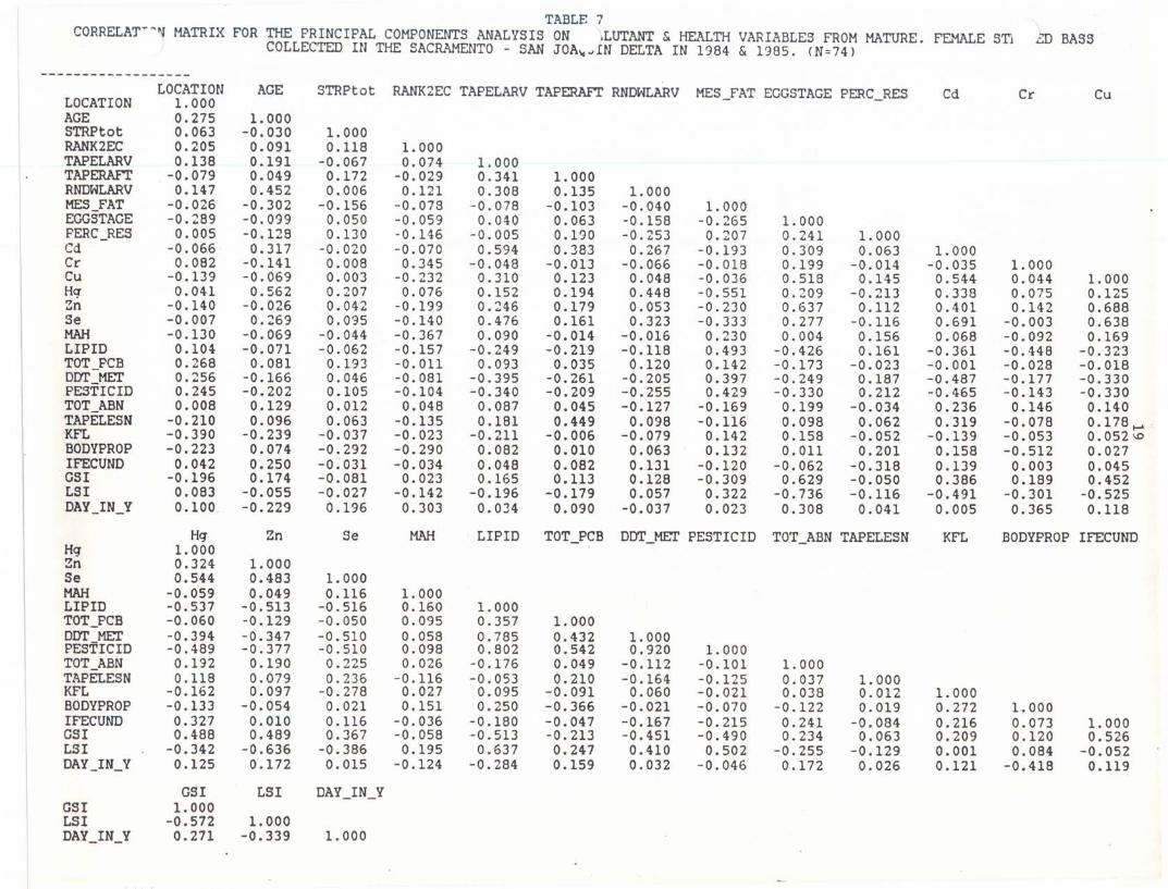
TABLE 7CORRELAT-~~ MATRIX FOR THE PRINCIPAL COMPONENTS ANALYSIS ON .LUTANT &. HEALTH VARBBLES FROM MATURE. FEMALE STI 2D BASSCOLLECTED IN THE SACRAMENTO - SAN JOA~~IN DELTA IN 1984 & 1985. (N=741

------------------LOCATION AGE STRPtot RANK2EC TAPELARV TAPERAFT RNDWLARV MES_FAT EGGSTAGE PERC_RES Cd Cr CuLOCATION 1.000

AGE 0.275 1.000STRPtot 0.063 -0.030 1.000RANK2EC 0.205 0.091 0.118 1.000TAPELARV 0.138 0.191 -0.067 0.074 1.000TAPERAFT -0.079 0.049 0.172 -0.029 0.341 1.000RNDWLARV 0.147 0.452 0.006 0.121 0.308 0.135 1.000MES FAT -0.026 -0.302 -0.156 -0.078 -0.078 -0.103 -0.040 1.000EGG STAGE -0.~89 -0.099 0.050 -0.059 0.040 0.063 -0.158 -0.265 1.000PERC_RES 0.005 -0.128 0.130 -0.146 -0.005 0.190 -0.253 0.207 0.241 1.000Cd -0.066 0.317 -0.020 -0.070 0.594 0.383 0.267 -0.193 0.309 0.063 1.000Cr 0.082 -0.141 0.008 0.345 -0.048 -0.013 -0.066 -0.018 0.199 -0.014 -0.035 1.000Cu -0.139 -0.069 0.003 -0.232 0.310 0.123 0.048 -0.036 0.518 0.145 0.544 0.044 1.000Hq 0.041 0.562 0.207 0.076 0.152 0.194 0.448 -0.551 0.209 -0.213 0.338 0.075 0.125Zn -0.140 -0.026 0.042 -0.199 0.246 0.179 0.053 -0.230 0.637 0.112 0.401 0.142 0.688Se -0.007 0.~69 0.095 -0.140 0.476 0.161 0.323 -0.333 0.277 -0.116 0.691 -0.003 0.638MAH -0.130 -0.069 -0.044 -0.367 0.090 -0.014 -0.016 0.230 0.004 0.156 0.068 -0.092 0.169LIPID 0.104- -0.071 -0.062 -0.157 -0.249 -0.219 -0.118 0.493 -0.426 0.161 -0.361 -0.448 -0.323TOT PCB 0.268 0.081 0.193 -O.Oll 0.093 0.035 0.120 0.142 -0.173 -0.023 -0.001 -0.028 -0.018DOT-MET 0.256 -0.166 0.046 -0.081 -0.395 -0.261 -0.205 0.397 -0.249 0.187 -0.487 -0.177 -0.330PESTICID 0.245 -0.202 0.105 -0.104 -0.340 -0.209 -0.255 0.429 -0.330 0.212 -0.465 -0.143 -0.330TOT_ABN 0.008 0.129 0.012 0.048 0.087 0.045 -0.127 -0.169 0.199 -0.034 0.236 0.146 0.140TAPELESN -0.210 0.096 0.063 -0.135 0.181 0.449 0.098 -0.116 0.098 0.062 0.319 -0.078 o .178 ~KFL -0.390 -0.239 -0.037 -0.023 -0.211 -0.006 -0.079 0.142 0.158 -0.052 -0.139 -0.053 0.052\0BODYPROP -0.223 0.074 -0.292 -0.290 0.082 0.010 0.063 0.132 0.011 0.201 0.158 -0.512 0.027IFECUND 0.042 0.250 -0;031 -0.034 0.048 0.082 0.131 -0.120 -0.062 -0.318 0.139 0.003 0.045GSI -0.196 0.174 -0.081 0.023 0.165 0.113 0.128 -0.309 0.629 -0.050 0.386 0.189 0.452LSI 0.083 -0.055 -0.027 -0.142 -0.196 -0.179 0.057 0.322 -0.736 -0.116 -0.491 -0.301 -0.525DAY_IN_Y 0.100 -0.229 0.196 0.303 0.034 0.090 -0.037 0.023 0.308 0.041 0.005 0.365 0.118

Hq Zn Se MAH LIPID TOT_PCB DOT_MET PESTICID TOT_ABN TAPELESN KFL BODYPROP IFECUNDHq 1.000Zn 0.324 1.000Se 0.544 0.483 1.000MAH -0.059 0.049 0.116 1.000LIPID -0.537 -0.513 -0.516 0.160 1.000TOT_PCB -0.060 -0.129 -0.050 0.095 0.357 1.000DOT MET -0.394 -0.347 -0.510 0.058 0.785 0.432 1.000PESTICID -0.489 -0.377 -0.510 0.098 0.802 0.542 0.920 1.000TOT_ABN 0.192 0.190 0.225 0.026 -0.176 0.049 -0.112 -0.101 1.000TAPELESN 0.118 0.079 0.236 -0.116 -0.053 0.210 -0.164 -0.125 0.037 1.000KFL -0.162 0.097 -0.278 0.027 0.095 -0.091 0.060 -0.021 0.038 0.012 1.000BODYPROP -0.133 -0.054 0.021 0.151 0.250 -0.366 -0.021 -0.070 -0.122 0.019 0.272 1.000IFECUND 0.327 0.010 0.116 -0.036 -0.180 -0.047 -0.167 -0.215 0.241 -0.084 0.216 0.073 1.000GSI 0.488 0.489 0.367 -0.058 -0.513 -0.213 -0.451 -0.490 0.234 0.063 0.209 0.120 0.526LSI -0.342 -0.636 -0.386 0.195 0.637 0.247 0.410 0.502 -0.255 -0.129 0.001 0.084 -0.052DAY_IN_Y 0.125 0.172 0.015 -0.124 -0.284 0.159 0.032 -0.046 0.172 0.026 0.121 -0.418 0.119

GSI LSI DAY_IN_YGSI 1.000LSI -0.572 1.000DAY_IN_Y 0.271 -0.339 1.000

between fish health and pollutant variables, there are no obvious

functional relationships among the variables.

The fifth component represents an association between lower

mesenteric fat abundance and greater concentrations of mercury in

older fish. Fish with these characteristics also tended to have

slightly higher selenium concentrations, slightly lower condition

factors (KFL) and slightly more broken striping pattern. This

component suggests that mercury accumulation in older fish may

lead to poor physical condition as represented by low mesenteric

fat and slightly lower than average weight proportional to their

length (KFL).

The remaining components represent very weak trends in the

data (Table 6 & 7). However, they present interesting

associations among the variables that should be considered as

working hypotheses. Component six indicates that fish with

_greater body-weight-corrected fecundity tend to have slightly

larger gonads (GSI), as would be expected; are in slightly better

condition (KFL); and have slightly less egg resorption. Component

seven shows an expected association between tapeworm lesions and

rafts, and indicates that they are slightly more common in fish

with a broken striping pattern from the San Joaquin River. In

component eight, fish with yellower egg color are slightly

associated with monocyclic aromatic hydrocarbons and the trace

metals copper and selenium. This last component is the only oneof the final three that suggests a relationship between pollutants

and fish health, implying that trace metals and monocyclic

aromatic hydrocarbons may be related to more immature (yellower)

egg color. Possibly, these compounds cause a delay in or

retardation of egg maturation.

It is unfortunate that stronger relationships among variables

could not be demonstrated with the 8-year data set, but the low

number of correlations exceeding 0.30 (Table 4) indicates that

there were not many strong, consistent relationships among

variables. Also, with only two pollutant variables (MAH and AH)

monitored consistently in all fish throughout all 8 years of the

study, there was not much potential for drawing conclusions about

toxicants and fish health. The last 2 years of the study show

some trends which, with 4 or 5 years of consistent results might

lead to a striped bass "health index" based on egg resorption,

condition factor (KFL), trace metal and pesticide concentrations,

and degree of parasitization.

Most fish collected after 1978 did not contain either

monocyclic aromatic hydrocarbons or alicyclic hexanes above the

limits of analytical detection (79% had no MAH, 84%, no AH);

therefore, there was little potential for measuring the effects of

these chemicals. Considering their high volatility and the rapid

depuration rates of monocyclic aromatic hydrocarbons by striped

bass (Korn et ale 1976 and Whipple et ale 1981), there may not be

much potential for measuring the effects of these compounds in

field-sampled fish. Effects of monocyclic aromatic hydrocarbons

and alicyclic hexanes may not be traceable because these chemicals

are depurated before the fish are sampled.

Actually, the problem of tracing effects may be common to

many toxic compounds. Fish may be exposed to pollutants during

any phase of their migration, experience chronic toxic effects,

and then excrete most or all of these compounds prior to our

sampling.

Egg resorption, a variable likely to reflect the impacts of

pollutants on reproduction, was not strongly related to any

chemical compound, although it was slightly correlated with the

fat soluble pesticides (PCB's and DDT and its metabolites).

Resorption was only vaguely related to monocyclic aromatic

hydrocarbons over the years (component #7, Table 3), and to

general condition of the fish (component #6, Table 6).

With the exception of component 2 from the 1984-85 data set

that accounted for 11.86%, the rest of the pollutant-health

components, individually, accounted for less than 10% of the

variability in the data matrix. While the amount of data

available normally would be sufficient to demonstrate strongrelationships, perhaps the observed concentrations of pollutants

had only very minor or subtle effects, or pollutants were no

longer present in fish tissues often enough or in concentrations

high enough to relate them to the physical condition of the fish

at the time of collection. These effects may not be obviouswithout more data. Principal Components Analysis is more robust

with more than 500 cases, but we only have 74 fish with a full

bass health. 3) We may have failed to measure the most important

pollutants since we do not test for all possible compounds. 4) Wemay have failed to select the best measures of striped bass

condition to reflect pollutant impacts.

I___________________ 1

Chatfield, C. & Collins, A. J. 1980. Introduction to

Multivariate Analysis. Chapman and Hall, London & New York.

Gauch, H. G. Jr. 1982. Multivariate Analysis in Community

Ecology. Cambridge University Press, Cambridge.

Jung, M., J. A. Whipple, and M. Moser. 1984. Summary Report of

the Cooperative Striped Bass Study. Institute for AquaticResources, Santa Cruz, CA., USA. 117 p.

Korn, S. N. Hirsch, and J. W. Struhsaker. 1976. Uptake,

distribution, an depuration of 14C-benzene in northern

anchovy, Enqraulis mordax, and striped bass, Morone

saxatilis. Fishery Bulletin, U.S. 74:545-551.

Knudsen, D. L. and D. W. Kohlhorst. 1987. Striped Bass Health

Index Monitoring 1985 final report. California Department ofFish and Game, Bay-Delta Fisheries Project, Stockton,

California; prepared for California State Water Resources

Control Baord under Interagency Agreement 4-090-0120-0.

141 p. (DFG Exhibit #47)

Pielou, E. C. 1984. The Interpretation of Ecological Data: A

Primer on Classification and Ordination. John Wiley & Sons,

New York.

Pimentel, R. A. 1979. Morphometrics: The Multivariate Analysisof Biological Data. Kendall/Hunt Publishing Company,Dubuque, Iowa.

Tabachnick, B. G. & Fidell, L. S. 1983. Using Multivariate

Statistics. Harper & Row, Publishers, New York.Whipple, J. A. 1984. The impact of estuarine degradation and

chronic pollution on populations of anadromous striped bass

(Morone saxatilis) in the San Francisco Bay-Delta,

California: A summary for managers and regulators. NMFS

Southwest Fisheries Center Administrative Report No. T-84-0l.

47 p.

Whipple, J. A., M. Jung, R. MacFarlane and R. Fischer. 1984.

Histopathological manual for monitoring health of striped

bass in relation to pollutant burdens. NOAA Technical

Memorandum. NMFS SWFC-46. 81 p.

Whipple, J. A., M. B. Eldridge, and P. Benville, Jr. 1981. An

ecological perspective of the effects of monocyclic aromatic

hydrocarbons on fishes. In F. J. Vernberg, A. Calabrese, F.

P. Thurberg, and W. B. Vernberg (editors), Biological

monitoring of marine pollutants, p. 483-551. Academic Press,N.Y.

Principal Components Analysis uses matrix algebra and eigen

analysis to summarize all of the variability in the original data

into independent dimensions called components. Principal

Components Analysis is used to summarize patterns of variability

in the data and not to test for statistical differences. The goal

of Principal Components Analysis is to extract the maximum

variance from the data set with each ~omponent. The first

principal component is the linear combination of observed

variables that maximally separates cases (data points) by

maximizing the variance of their component scores. The second

component is formed from variability remaining in the data set

after the variance associated with the first component is removed;

it is the linear combination of observed variables that extracts

maximum variability from the data uncorrelated with the firstcomponent. Each component is uncorrelated with every other

component and there are as many of them computed as there are

original variables used in the analyses (i.e., if eight variables

are analyzed, eight components are produced). Since each

component is statistically independant, it represents a unique and

independant trend among the variables represented in the original

data. For a complete explanation of the computations involved in

Principal Components Analysis see Chatfield & Collins 1980 or

Tabachnick and Fidell 1983, and refer to Gauch 1982, Pielou 1984,

or Pimentel 1979 for its application to biological data.

The use of Principal Components Analysis assumes that most of

the variability in the data will be accounted for by relatively

few independent trends (components) common to the variables

measured, so not all of the components extracted from the data are

rotated to enhance their interpretation. Rotation is the process

of adjusting the fit of those components chosen for interpretation

to the data in order to maximize the correlations between the

original variables and these components. The process of rotation

also simplifies the interpretation of ~he analyses by making each

variable correlate with as few components as possible. Thecorrelations between the original variables and these new rotated

components computed from them are found in what is called the

"Pattern Matrix" or the "Loading Matrix" for the rotated

components. The interpretation of this matrix allows the

statistical analyst to decide which of the original variables were

intercorrelated and have common patterns of variability. Matrices

for our two analyses are found in Tables 3 and 6. The components

were rotated orthogonally to retain the statistical independence

of each component and because oblique rotations, which allow

components to be intercorrelated, are difficult to analyze and

explain. The techniques for choosing which components to rotate

and interpret are discussed after the following section on the

nature of the raw variables and their transformations to meet the

assumptions of Principal Components Analysis.

Two different Principal Components Analysis's were examined:

one for the data in 1984 and 1985 where all variables were

measured on the majority of fish collected, and one over all 8

years of the study using the 17 variables that were measured inall fish in all years. Data screening was performed on each

variable using the whole data set if it was to be used in the

analysis of the whole study, and separately using only the 1984-85

data if it was to be used in the analysis of those years.

Since Principal Components Analysis does not test for

statistical significance, its assumptions are less restrictive

than those of most other parametric, multivariate techniques (see

Tabachnick & Fidell, 1983). If the technique is being used to

simply describe the data, as in this study, and not to testassumptions about the number of components, then even the

assumptions of multivariate normality and linear relationshipsamong variables can be relaxed. If variables are univariate andmultivariate normal in distribution with linear relationships

between them, then the outcome and fit of the analysis isenhanced. To the extent that normality and linearity fail, theresult is degraded, but still may be worthwhile.

The assumptions of multivariate normality and colinearity

among variables cannot be tested directly. Using variables thatare univariate normal (or transformed to approximate it) and

eliminating multivariate outliers from the data will probably

assure multivariate normality. If variables were not normally

distributed, their scales were transformed to meet or approximate

normality. The variables used in the analyses, their scale, and

transformations, if any, are shown in Table 1, which also

indicates their relative degree of normality and in which

Principal Components Analysis they were used. Multivariate

outliers were eliminated based on their Maha1anobis distances from

the multivariate mean (centroid) of all the data. Nine data cases

were eliminated from the analysis of 8 years of data because theyhad less than one chance in a thousand of being representative of

the data as a whole (p(O.OOl). A stricter criteria (p(O.Ol) was

applied to the smaller data set for 1984-1985 and two cases were

eliminated. Bivariate scatterp10ts of selected variables

(transformed if necessary) were used to asses their bivariate

normality and implied co1inearity. No departure from linearity

was obvious so all variables were assumed to be linearly related.

It would be best to use only variables which were continuous

and had interval or ratio scales of measurement for Principal

Components Analysis, since they provide the most precise measures

of variability. However, some of the variables were ranked

variables with ordinal scales of measurement. Using these ranked

variables is valid, especially when Principal Components Analysis

is used to summarize the patterns in the data. Ranked variables

are commonly used by psychometricians in Principal Components

Analysis and Factor Analysis to test hypotheses and develop

theory. Ranked variables were used where it was impractical to

measure on a finer scale or where there was no accepted standard

scale of measurement for the feature which we wished to quantify.

The Principal Components Analyses were done on the

correlation matrix instead of the sum of squares and cross

products matrix because the former is equivalent to analyzing

Z-transformed variables. This approach was necessary because all

the variables were not in the same units (i.e. counts) and did not

have similar variances.

There are three methods of selecting how many components to

extract from the data and rotate for best fit prior to

interpretation. 1) At most, only those unrotated components with

an eigenvalue L 1 would be selected, because those witheigenvalues ( 1 represent less of the variability in the data than

a single original variable. 2) Evaluate those components screened

by the first method for the percent of total variance extracted by

each of them. Components that extract less than 5% of the total

variance in the data, especially after rotation, obviously do notcontain much meaningful information and could be eliminated from

further consideration. Another way of assessing the value of each

unrotated component is to plot the percent of variance extracted

by each component from the first to the last component as a curve

and to use only those components before the point at which the

curve levels off. This is known as Catell's Scree Test and is

based on the fact that, after the first few meaningful components

have been computed, the rest of the components will tend to

account for similar but gradually decreasing proportions of the

total variance. 3) A final and conservative evaluation is to

examine the sorted and shaded correlation matrix among the

variables sorted by classification analysis. This matrix tends to

group variables according to their associations and graphically

demonstrate strong trends. This matrix is interpreted by

qualitatively examining it for the number of strongly related

groups of variables. Figure 3 is the best example included in

this report and I have labeled the five groups I was able to

differentiate in the matrix. The first two groups are obvious and

strongly interrelated, with many variables correlated at r 1

0.690. The next three groups are less apparent and based on

weaker correlations, often with r i 0.575. The number of visible

groups, based on a qualitative inspection, should equal the number

of strong components, and one should not interpret too many more

components than this since the standard matrix indicates those

groups for which there are very strong bivariate correlations.

Even after selecting components for extraction and rotation

with these techniques, it is necessary to evaluate the reliability

of each component to ensure a parsimonious interpretation of the

results. Components should have three or more variables

correlated with them at levels >0.50 for them to be consideredreliable. A component with only two variables strongly correlated

with it is no better than a bivariate correlation and when only

one variable is strongly correlated with it, may simply represent

a variable which is unrelated to any other in the data set. The

interpretation of components correlated with less than three

variables (at r)0.50) should be done cautiously and be supported

by the interpretation of the bivariate correlation matrix.

Variables which correlate with components at <0.316 should

probably not be interpreted except with much larger data sets

(300-500+ cases).

Reliable components also are most likely to be produced when

an analysis has many more data points than variables used in the

analysis or components interpreted. Since both data sets are

small (8 yrs=199 cases, 1984-85=74 cases), it is important not to

interpret too many components or use too many variables. This

study has restricted the analyses to the smallest set of

meaningful variables possible by combining all monocyclic aromatic

hydrocarbons into one variable, and doing the same for pesticides.

This method is especially appropriate for the pesticides since

they are all intercorrelated and tend to be associated with asimilar set of variables.