The Regulatory Environment, Relative PriceEfficiency and the Egyptian Private

Manufacturing Sector: 1987/88-1995/96∗

Lullit GetachewPacific Economics GroupMadison, Wisconsinlullit@yahoo.com

Robin C. SicklesDepartment of Economics

Rice Universityrsickles@rice.edu

September 1, 2003

Abstract

We study the impact of regulatory and institutional distortions, andreforms instituted to remedy them on the private manufacturing sectorof Egypt. We undertake this study using a generalized cost function,which subsumes the standard neoclassical cost function as a specialcase. This approach allows us to assess the impact of institutional andregulatory restraints on the structure of production, including factordemands, total cost and scale economies. Our findings indicate thepresence of substantial distortions in relative prices, and hence on op-erating efficiency, due to the binding contraints. In addition, we findthat these inefficiencies are magnified among large firms. We also findimprovements in efficiency after the reforms were initiated.

Keywords: Productivity, generalized cost function, gmm, economicdevelopement.JEL Classification: D24, C30, O10.

∗The authors would like to thank members of the Development Economic Policy Re-form Analysis Project (DEPRA), USAID/Egypt and the Ministry of Economy of Egypt(Contract No. 263-0233-C-00-96-00001-00). The second author was the project’s SeniorResearch Coordinator. The authors also thank Dr. Suzanne Messiha and the CompTeamfor their valuable suggestions and contributions to the collection and oversight of all thedata series on which this paper is based. Bryan W. Brown and Mahmoud El-Gamal pro-vided needed criticisms and insights. The research and findings do not necessarily reflectthe opinions or conclusions of Nathan Associates, USAID or the Ministry of Economy ofEgypt. The usual caveat applies.

1

1 Introduction

As Tybout (2000) indicates, many observers have come to believe that thecomplex system of regulations and bureaucratic burdens are major obsta-cles to the development of the manufacturing sector in many developingcountries. This is true of Egypt where such institutional constraints havehampered the activities of the private sector, in general, and the privatemanufacturing sector, in particular. In this study we analyze the impact ofregulatory and institutional distortions on the Egyptian private manufac-turing sector from the mid 1980s to the mid 1990s. We study the impactof economic reforms, undertaken since 1991, on the sector’s performance byexamining productive peformance in the pre and post reform periods. Wealso examine the impact of distortions by the size of the enterprise.

The literature on the impact of regulation on optimizing behavior is use-ful in the analysis of the structure of production where producers are likely toface binding constraints on their decision making. It extends duality theoryby incorporating the impact of such constraints on firm behavior. Generallythe dual representation of production allows the use of flexible functionalforms and through simple derivation, the use of a system of input demandequations to study production technology. The standard neoclassical costfunction used by this approach rests on the assumption of cost minimizingbehavior given market prices on the part of producers. However, in thepresence of regulatory, or related constraints in the operating environment,the assumption of cost minimization given market prices is unlikely to hold.Instead, the use of a generalized cost function which incorporates the im-pact of such distortions is a more useful approach. This approach, whichincorporates optimizing behavior subject to shadow prices that deviate frommarket prices due to distortions in the operating environment, reveals theextent and directions of such distortions. It also indicates the impact of suchdistortions on various cost characteristics including scale economies, totalcost and factor shares. Such distortions caused by constraints imposed bythe operating environment alter firm behavior enough to result in changesin their cost characteristics and production technology.

In the next section, we detail the institutional background of the study.This is followed by section 3, where we present the generalized cost functionand the empirical specification, and section 4 where we describe the data.We present empirical results in section 5 and concluding remarks in section6.

2

2 Institutional Background

2.1 The Private Sector

Throughout the study period, but to a decreasing extent over time, Egypt’sprivate sector boundaries have been limited. The state has been presentin many areas of economic activity, either as a monopoly or as the largestplayer. Overall, four types of public institutions have been present in theeconomic arena: local government ventures, service and economic authori-ties - which operate in the areas of public utilities, insurance, the Suez Canaland the Petroleum Company, and the General Authority for Supply of Com-modities that imports and distributes necessities - and public enterprises.The latter, although not legally granted monopolistic rights, have operatedin almost all productive activities ranging from cement, iron and hotels, anddominate the Egyptian financial system.

Despite the heavy presence of these public enterprises, Egypt’s privatesector comprises participants ranging from formal medium and large en-terprises (MLEs) to micro or small ones (MSEs). Those considered smallemploy less than 10 workers, medium enterprises employ 10 to 99 peopleand large enterprises employ 100 and more persons. The MLEs are well con-nected, institutionally visible, protected, with access to all the institutionalprivate credit, and are incorporated into legal forms, including joint-stockcompanies and limited liability establishments. They use relatively advancedtechnologies, make most of the country’s private investments and contributemost to its private exports. The MSEs, on the other hand, are largely infor-mal, are set up as single proprietorship or informal partnerships, are finan-cially constrained and inconsistently regulated. They do turn out, however,most of the private sector’s output, and provide most of its jobs. They arealso the largest in number, constituting 99% of private non-agricultural and90% of agricultural establishments. In general, the private sector providesmost of the employment in Egypt, in fact over two thirds of total employ-ment, and pays marginally better salaries than the public sector: on average,US $565 per year for a private sector job versus US $536 per year for a publicsector one in FY 1992 (World Bank, 1994).

The private sector is classified into three sub-sectors: the formal, theinformal and investment sectors. Firms incorporated under law 159/1981fall under the private formal and those established under investment law230/1989, now amended as law 8/1997, fall under the investment sector.The latter sector is more export oriented than the other two, accounting for64% of total private industrial exports in 1995/96, while the formal and in-formal private sectors accounted for 11% and 25% of such exports in 1995/96,respectively. The difference between the formal and investment sectors fromthe informal sector is that the former need to maintain organized accountingpractices and submit reports for auditing, and are regulated by the invest-ment law for investing local and foreign capital and for doing so in the free

3

zones. The informal sector largely contains the MSEs.Private sector presence in the industrial sector, which includes both man-

ufacturing and mining and quarrying, has grown since the early 1990s. Totalprivate output by the industrial sector increased from 45% of the total in1992 to about 50% in 1996 (World Bank, 1994, p. 26), while employment inthe sector rose from 32% to 40% over this same period. Industry’s share oftotal GDP rose from 9% to over 14%, while the private manufacturing shareof GDP rose from 4.2% to over 7% over the same period.1 The formal sectordominates private industrial activity accounting for about half its output,at factor cost. The investment and informal sectors make up the remain-ing half, each accounting for around a quarter of the total.2 The informalsector, however, employs about 58% of total private industrial labor force,while the formal and investment sectors employ 20% and 22% of the totalrespectively.

2.2 The Business Environment

An array of factors constrains private sector development in Egypt. Theseinclude legal, regulatory, bureaucratic systems, and tax administration. TheCountry Commercial Guide of Egypt (1999) points to red tape as “a keybusiness impediment in Egypt, including a multiplicity of regulations andregulatory agencies, delays in clearing goods through customs, arbitrarydecision-making, high market entry transaction costs, and a generally unre-sponsive commercial court system.”3 The legal, regulatory and bureaucraticsystems factor in as large sunk costs of business by incumbents. These im-pede contestability by discouraging potential marginal entrants, who factorthese costs against the profitability of possible projects.

Among the areas most cited as hindering private business interests aresecuritization, tax and labor laws. Securitization laws, set by the Com-mercial Code of 1883, and only recently replaced by the Commercial Lawof 1999, place excessive limits on securitization, hindering firms’ ability toraise funds (Nathan Associates, 2000). The most serious problem of the tax-

1These are based on results in Nathan Associates, 2000, pp.11&13.2The large contribution to output by medium and large enterprises in the industrial

sector, which constitute the majority of the formal and investment sub-sectors, is unlikethe case in the other sectors of the economy where MSEs dominate.

3Corruption is part of the red tape that impedes business activity. The CorruptionPerceptions Index (CPI) compiled by CeGE of Goettingen University and TransparencyInternational, non-governmental organizations, indicates its extent. The CPI is basedon surveys from seven independent institutions and reflects the perceptions of businesspeople, academics and country analysts. It ranges from 10 (highly honest) to 0 (highlycorrupt). Historical data shows the CPI to be 1.12 for 1980-85 and 1.75 for the 1988-92period for Egypt indicating extensive corruption. The score has improved since the mid1990s: It was 2.84 for 1996, 2.9 for 1998, 3.1 for 2000 and 3.6 for 2001, all fiscal yearsending in June.

4

ation system is the unlimited discretionary powers granted to tax collectors.The absence of an independent tax appeal system, rewarding tax collectorsfor the revenues they bring and granting them the ability to assess liability,instead of auditing taxes filed, creates major barriers to investment by theprivate sector (Giugale and Mobarak, 1996).

Aside from tax administration, which is inefficient and cumbersome, thetax structure itself deters the level of investment. El Samalouty (1999)cites the application of high and numerous tax rates to a narrow base asdistortionary and a hinderance to growth in the private sector. It is true thatthe tax schedule applicable in our study, the unified income tax on corporateand non-corporate firms, favors manufacturing versus non-manufacturingfirms; the marginal effective tax rate (METR) is lower for the former at26.4% versus for service firms at 37.3%. Firms are not, however, allowedto receive input tax credits under the sales tax for the purchases of capitalgoods, which adds 5% to 10% to the METR and hence lowers investment.Firms’ optimization decisions are thus affected by such tax considerations.

Labor laws dictate, to a great detail, personnel management and areobstacles to labor mobility. Ibrachy (1996) outlines the difficulties posed bythe unified labor law, Law 137 of 1981, which biases business activity awayfrom labor-intensive processes. Once a worker is hired, the law makes it verydifficult to terminate the contract. Dismissal requires that the employersubmits a request to a tripartite consultive committee, which is often timeconsuming and futile. Aside from such firing difficulties, employers oftenface administrative pressure in the hiring process since the law does notshield them from this; in particular, public administrative authorities havethe power to suggest a person for a job. In addition, the law does not allowemployers to reallocate workers to different areas in case of need. Further,in addition to extended annual and weekly vacation and public holidays, thelaw does not allow incidental leave to be deducted from annual leave. Thishas serious consequences for productivity. The law also dictates that privatesector employees receive an annual raise of 7 percent, in keeping with suchraises in the public sector. These hiring, firing, reallocating, leave and payproblems pose hidden labor costs that alter labor demand among privatemanufacturing firms.

In addition, high tariff and non-tariff barriers to trade, and energy poli-cies have distortionary impact on input use in the private manufacturingsector. For instance, tariff rates in excess of 70% existed prior to 1991. Sincemost capital goods are imported, the imposition of excessive customs dutieson these goods further aggravates the problem posed by the tax system. (ElSamalouty, 1999). Energy policy in Egypt, in line with those found in manydeveloping countries, has favored energy subsidies to protect the poor andinfant industries.4 Such subsidies are not budgetary, but are achieved by

4Generally, such policies do not have the intended impact of protecting the poor andinfant industries. Most often they protect those that would have purchased energy at the

5

price regulation. Specifically, price ceilings keep retail prices of petroleumproducts, in most categories, and natural gas below their economic value, oropportunity cost, as measured by their prices in the world market (WorldBank, 1998). These policy measures have serious implications for relativeprice efficiency.

Relevant reforms in these and related areas have been implemented sincethe early 1990s. We briefly outline these reforms next.

2.3 The Reforms

Egypt initiated its structural adjustment program at the start of 1991. Ingeneral, the aim of the reforms was to orient the planned economy to-wards one led by a private sector market economy. Initial efforts focused onmacroeconomic stabilization. Essentially, these focused on the reduction ofthe fiscal deficit through cuts in public investment and subsidization pro-grams, tax reforms, particularly through the introduction of a general salestax and improvements in collection, and monetary policy tightening to fightinflation.

The authorities also undertook extensive price liberalization and adjust-ments of relative prices. In particular, they freed prices of products thatwere under high trade protection and of specific goods controlled by theMinistry of Industry, including animal feed and cotton. They also raisedthe prices of many administered goods and services closer to their economicvalue, including those of pharmaceuticals, cement, cotton and energy prod-ucts (World Bank, 1994).

Along with price liberalization, trade and financial sector reforms werealso instituted. On the trade front, tariff rate dispersions were reduced to 5to 70% bracket, all export quotas, except for tanned hide, were removed. Inaddition, tariffs on almost all imported capital goods were lifted (Develop-ment Economic Policy Reform Analysis [DEPRA] Report, 1998). Financialsector reforms include the removal of nominal interest rate ceilings, adminis-trative credit allocation, foreign exchange controls and prohibitions againstinternational capital mobility (World Bank, 1994).

Labor law reforms were also initiated, including those that allow em-ployers the right to hire and lay off workers in accordance with economicconditions. These reforms are part of secondary structural reform efforts,following the initial stabilization policies already outlined (IPR CountryGuide, 1998).

Although problems remain in these areas, assessing the impact of bur-dens of doing business on efficiency, both within the pre- and post-reformcontexts is informative. It reveals the extent of impediments resulting fromsuch burdens. Moroever, modeling each specific constraint formally is prob-lematic, not least because the constraints are difficult to quantify and mea-

unsubsidized prices.

6

sure. To undertake this assessment, we use the generalized cost functiondeveloped in the next section.

3 The Generalized Cost Model

3.1 The Model

The generalized cost model, subsuming the standard neoclassical model asa special case, is developed in Atkinson and Halvorsen (1984) and Evanoff,Israilevich and Merris (1990). In addition, Good, Nadiri and Sickles (1991,1997) develop a similar model which differs in the specification of shadowprices. The standard neoclassical cost function is based on the assumptionthat firms minimize cost subject to an output constraint:

minX

C = P 0X s.t f(X) ≤ Q (1)

where Q and X are h × 1 vectors of price and quantity of inputs, f(X) isa well behaved production function and Q is output.5 The Lagrangian forthe firm’s constrained cost minimization is then

L = P 0X − υ(f(X)−Q) (2)

and from the first order conditions for cost minimization we obtain

PiPj=

fifj

for i 6= j = 1...h (3)

The equality of the marginal rate of technical substitution to the ratio of themarket price of inputs gives the optimal combination of inputs that minimizecost.6

Now suppose Rk, k = 1...n, additional constraints exist due to the regu-latory environment. The regulatory constraint can be written asR(P,X, φ) ≤0 where R is the n-dimensional vector, with n < h− 1, and φ is a vector of

5 In particular, the production function is assumed to be twice continously differentiable,(f ∈ C2), monotonic, ( ∂f

∂X≥ 0) and quasi-concave (θ 6= 0 and ¡ ∂f

∂X

¢0θ = 0, which implies

θ0¡∂2f∂X2

¢θ ≤ 0. Here θ is h× 1 vector).

6These input demand functions are assumed to be continuously differentiable , ∂X∂P

∈C1, homogeneous of degree zero in P , and to have a symmetric matrix of price effects,(∂X∂P =

¡∂X∂P

¢T), which is negative-definite, θ0 ∂X∂P θ < 0. The associated cost function is

then assumed to be twice continuously differentiable, C ∈ C2, increasing in (P,Q) ormonotonic, concave in P , ∂2C

∂P2< 0, homogeneous of degree one in P and having the

derivability property (Shepard’s Lemma) ∂C∂P

= X.

7

regulatory parameters. (Lasserre and Ouellette,1994)7 With the additionalconstraint due to the regulatory environment, the firm’s cost minimizationproblem becomes

minX

C = P 0X s.t. f(X) ≤ Q and R(X,P ) ≤ 0 (4)

The Lagrangian for the firm’s constrained optimization then becomes

L = P 0X − υ(f(X)−Q)−nX

k=1

λkRk(P,X) (5)

where λk, k = 1...n, are now the Lagrangian multipliers associated with then additional constraints. The first order conditions for cost minimizationnow give

fifj=

Pi +Pn

k=1 λk∂Rk∂Xi

Pj +Pn

k=1 λk∂Rk∂Xj

=P ei

P ej

i 6= j = 1...h (6)

The marginal rate of substitution is equated to the ratio of shadow or ef-fective prices in this case and implies a cost function different from the oneimplied by the first order conditions in the standard neoclassical case whenregulatory constraints are binding; otherwise, (6) implied by the first orderconditions is the same as that of the neoclassical case where the marginalrate of substitution is equated to the ratio of market prices. In our study,the specification of the constraints is a problem since the arguments of theregulatory constraint are not well defined; given that we are studying thedistortionary impact of institutional constraints on the private manufactur-ing firms, we can not explicitly specify them in (6). But the extent to whichwe can estimate parameters of shadow prices allows us to determine theirbinding constraint on firm decision making and identify the magnitude ofthe divergence of shadow from market prices.

As a first step in estimating the parameters of the unobservable shadowprices, Lau and Yotopolous (1971) and Atkinson and Halverson (1984) ap-proximate these shadow prices by

P ei = kiPi, i = 1...h (7)

where ki is an input specific factor of proportionality. This approximationcan be interpreted as a first order Taylor series approximation to a general

7 In the rate of return regulation, where this type of analysis has been extensivelyapplied, for instance, R(·) = TR−P 0X−sk, where TR is total revenue and the argumentof the regulatory constraint φ = s. For quantity standards regulation R(·) = X ≤ φ andfor input price regulation, R(·) = P ≤ φ. As a result, the details of regulation need notbe known, just the arguments.

8

shadow cost function gi(Pi), with the properties that gi(0) = 0 and∂gi(Pi)∂Pi

≥0.

The shadow cost function, which differs from the neoclassical cost func-tion only in the input price variable, is given by

CS = CS(kP,Q) (8)

The logarithmic differentiation of the shadow cost function yields the shadowshare for input i

∂ lnCS

∂ ln kiPi=

∂CS

∂kiPi∗ kiPiCS

, i = 1...h (9)

From Shepard’s Lemma,

∂CS

∂kiPi= Xi, i = 1...h (10)

=⇒ ∂ lnCS

∂ ln kiPi= Xi ∗ kiPi

CS=MS

i , i = 1...h (11)

=⇒ Xi =MSi C

S(kiPi)−1, i = 1...h (12)

The firm’s actual cost function is

CA =hXi=1

PiXi, i = 1...h (13)

Using (12), we get

CA =hXi=1

Pi ∗MSi C

S(kiPi)−1, i = 1...h (14)

=⇒ CA = CShXi=l

MSi (ki)

−1 (15)

Taking log of (15) yields

lnCA = lnCS + lnhXi=1

MSi (ki)

−1, i = 1...h (16)

The actual share equation for input i is

MAi =

XiPiCA

, i = 1...h (17)

9

Using (12) and (15), this becomes

MAi =

MSi C

S(kiPi)−1Pi

CSPh

i=1MSi (ki)

−1 , i = 1...h (18)

=⇒MAi =

MSi (ki)

−1Phi=1M

Si (ki)

−1 , i = 1...h (19)

3.2 Empirical Specification

Using the translog functional form, which provides a second order approxi-mation to an arbitrary continuously twice differentiable function, we writethe shadow cost function as:

lnCS = αo + αQ lnQ+ 1/2γQQ(lnQ)2 +

Xi

αi ln(kiPi)

+Xi

γiQ lnQ ln(kiPi)+1/2Xi

Xj

γij ln(kiPi) ln(kjPj)+δt ln(t), i, j = 1...h

where symmetry restrictions γij = γji are imposed. All variable descriptionsare as above and t is time trend used to proxy disembodied technologicalchange. The shadow cost function has the same properties as the neoclassicalcost function, one of which is linear homogeneity in shadow prices. Thisimplies the following parametric restrictionsX

i

αi = 1,Xi

γiQ = 0,Xi

γij =Xj

γij =Xi

Xj

γij = 0 (20)

From the logarithmic differentiation of the shadow cost function, we obtainthe shadow share for input i to be the following

MSi =

∂ lnCS

∂ ln kiPi= αi + γiQ lnQ+

Xj

γij ln(kjPj), i, j = 1...h (21)

The actual cost function then becomes

lnCA = lnCS+ln

Xi

αi + γiQ lnQ+Xj

γij ln(kjPj)

k−1i

, i, j = 1...h

(22)and the corresponding actual cost share of input i becomes

MAi =

³αi +

Pj γij ln(kjPj) + γiQ lnQ

´(ki)

−1Pi

³αi +

Pj γij ln(kjPj) + γiQ lnQ

´(ki)−1

, i, j = 1...h (23)

10

We also obtain further summary statistics from parameter estimates ofthe actual cost function and its associated share equations by calculatingprice elasticities of demand and the Allen-Uzawa partial elasticities of factorsubstitution. The Allen-Uzawa cross and own elasticities of substitution aregiven by:

θij =γij +MiMj

MiMj(24)

θii =γii +Mi(Mi − 1)

M2i

(25)

The cross and own price elasticities are given by:

∈ij= θijMj (26)

∈ji= θijMi (27)

∈ii= θiiMi (28)

3.3 Estimation

Estimation is based on a four factor input nonlinear cost function and the as-sociated factor share equations. For this type of cost share model, the usualpractice in empirical work with regards to the stochastic structure involvesappending well behaved error terms to the system of equations; estimation isundertaken with additive, homoscedastic error terms. Such practice allowsthe use of conventional estimators and distributional assumptions. Brownand Walker (1995), however, indicate this approach results in theoreticallyinconsistent models of stochastic behavior. The use of simple additive er-rors either leads to violations of homosecdasticity, or restricts the form ofthe underlying technology by limiting the set of distributions from which itis drawn.

A model of random rational behavior requires that firms minimize costsubject to market forces in input and output markets and to some techno-logical constraint. In our case, we also assume that additional constraintsin cost minimization arise from the operating environment. The randomvariation in this process could be due to factors unobservable to the econo-metrican, but known to the firms, or due to optimization errors.

Brown andWalker (1995) outline the necessary theoretical restrictions onrandom production models where the randomness arises from the productiontechnology. Under such a scenario, the optimization problem of firms is:

minX

P 0X s.t. f(X, ε, β) ≤ Q (29)

11

where all variable definitions are as before, and β and ε are vectors of param-eters and random variables respectively. The cost function that results fromthis constrained optimization must satisfy the restrictions outlined in foot-note 5. These restrictions are important in defining stochastic specificationsthat are consistent with the random production model.

From the cost function, C(P, Y, ε;β), we can either obtain input de-mand equations, Xi = fi(P, Y, ε;β) from ∂C(·)/∂Pi, or input share equa-tions, Si = gi(P, Y, ε;β) from ∂ ln(C)/∂ ln(Pi). A simple stochastic specifi-cation for the input demand model is not compatible with the assumptionof random optimization models. For example, consider the simple stochasticspecification:

Xi = fi = f i(P, Y ;β, η) + ui(ε;β, η) (30)

where η signifies a vector of shape parameters for the distribution of ε,f i = E[fi(·)|P, Y ) and ui = fi(·) − f i(·) is the disturbance term. GivenXi ≥ 0, f i + ui ≥ 0 and ui ≥ −f i, the non-negative inequality constraintimplies that the disturbances ui have bounds that are functions of P and Y .Therefore, ui will also be functionally dependent on P and Y or will have tocome from distributions that have limited support. If we do not restrict theset of distributions from which ui come, they are functionally dependent onP and Y such that:

Xi = fi = f i(P, Y ;β, η) + ui(P, Y, ε;β, η) (31)

As a result, the stochastic specification of the input demand system will notbe characterized by a simple additive and homoscedastic error term. It isalso possible to show the same outcome for the case where the randomnesscomes from random parameters, which reflect variation in behavior acrossfirms.

Similarly, for the cost share model, a simple stochastic specification willnot be appropriate. We can write the simple stochastic share equation as:

Si = gi(P, Y ;β, η) + vi(ε;β, η) (32)

where gi = E[gi(·)|P, Y ] and vi = Si−gi(·) is the simple additive disturbanceterm. Since gi(·) = ∂G1(·)/∂Pi and vi(·) = ∂V1(·)/∂Pi, we can write the(natural) log cost function from which Si comes as:

ln(C) = G1(P, Y ;β, η) + V1(ε;β, η) +K(Y, ε;β, η) (33)

where K(Y, ε;β, η) is a constant of integration. We can rewrite the costfunction as:

ln(C) = Go(Y ;β, η) +G1(P, Y ;β, η) + Vo(Y, ε;β, η) + V1(P, Y, ε;β, η) (34)

12

where Go(Y ;β, η) = E[K(Y, ε;β, η)|Y ] and Vo(Y, ε;β, η) = K(Y, ε;β, η) −Go(Y ;β, η).

8 A simple transformation of the cost function will give us a costshare system with homoscedastic disturbances:

Si = gi(P, Y ;β, η) + vi(ε;β, η) (35)

ln(C)−nXi=1

Si ln(Pi) = Go(Y ;β, η) +nXi=1

gi(P, Y ;β, η) ∗ ln(Pi) (36)

+G1(P, Y ;β, η) + vo

However, just as with the non-negative restrictions for the input demandsystem, there are restrictions on the cost shares: the unit simplex inequalityrestrictions of 0 ≤ Si ≤ 1 =⇒ 0 ≤ gi + vi ≤ 1 =⇒ −gi ≤ vi ≤ 1− gi. Againthe bounds of the inequalities are functions of P and Y , and thus vi willeither come from a restricted set of distributions with limited support or isfunctionally dependent on P and Y . This implies:

Si = gi(P, Y ;β, η) + vi(P, Y, ε;β, η) (37)

and hence disturbance terms that are no longer additive and homoscedas-tic. In fact, E(V V 0) = Ω(P, Y ;β,Σ) where Σ = E(εε0), which shows thedisturbances to be conditionally heteroscedastic.

For the cost share model used in this study we can transform the (nat-ural) log cost function as shown earlier and estimate the system of equa-tions if we are willing to tolerate violations of the unit simplex inequalityrestrictions. Although this does not alleviate the problem of conditional het-eroscedasticity it is possible to estimate the model ignoring the restrictionsbut using a heterosecdasticity corrected covariance matrix (HCCM) so thatthe standard errors are consistent. In keeping with the approach suggestedby Brown and Walker (1995), we utlize a GMM estimator that allows forefficient estimation in the presence of such heteroscedasticity.

Consider the following non-linear model:

Yit = h(Xit, β) + εit t = 1...T i = 1...n (38)

where β is a k × 1 vector of regressors, n is the number of equations and tis the number of observations. In the presence of conditional heteroscedas-ticity due to the functional dependence of the disturbances on the regres-sors and/or autocorrelation, we can set up orthogonality conditions usingL instrumental variables, zt = Z(Xit) that are uncorrelated with regres-sors. Identification of the parameters requires L = k, the exactly iden-tified case, or L > k, the overidentified case. Rewriting the models as

8Here V1(·) =nPi=1

vi(ε;β, η) ∗ ln(Pi) and we have the ln(Pi) multiplicative term to get

the vi(ε;β, η) term of Si from ∂ ln(C)/∂ ln(Pi).

13

εit(Yit,Xit, β) = Yit − h(Xit, β), we obtain the sample moment conditionsfrom:

m(β) =1

T

TXt=1

ztεit(Yit,Xit, β) (39)

=1

TZ 0ε(Y,X, β)

The GMM estimator bβGMM , comes from minimizing the criterion:

q =

·µ1

T

¶ε(Y,X, bβ)0Z¸V −1 ·µ 1

T

¶Z 0ε(Y,X, bβ)¸ (40)

where V is the variance matrix of the moment functions and is:

V =1

T

TXt=1

TXj=1

cov(ziεit, ziεjt) (41)

=1

TZ 0ΩijZ

We first obtain consistent estimates of bβ using NL2SLS and compute bV −1using the Newey-West (1987) estimator, and then minimize the criterionfunction to get bβGMM . Since the first order conditions are non-linear func-tions of the parameters, optimization can be done in different ways. Herewe adopt the Gauss-Newton method. (Greene, 2000). Given our model,the conditional mean of Yit given Xit is E(Yit|Xit) = h(Xit, β). The partialderivatives of this conditional mean with respect to the parameter vectorserve as efficient instrumental variables. (Ruud, 2000). The derivatives inthe sample moment conditions are thus constructed and the efficient GMMestimator eβGMM by minimizing the above criterion function using theseadditional orthogonality conditions.

4 The Data

We provide data sources and construction details in Appendix I. Using thesources and methods described in the Appendix, we constructed a paneldata of input and output quantities and prices covering nine years for theprivate manufacturing sector. At the two digit ISIC level, we have ninecross sections while at the three digit ISIC level, we have twenty-eight crosssections. Generally, to construct quantity and price indices for the outputand inputs, at the three digit level, first we compute the price index series,with base year 1987/88, by taking a weighted sum of the appropriate defla-tors for each sector; we use expenditures shares as weights. We then divide

14

the values of output and input by the appropriate price index to obtain aquantity index.

We have one measure of output, four measures of input quantity indicies,and their corresponding price indicies. Our input measures include mate-rials, energy, capital and labor. Their expenditure shares in total cost are16% for capital, 10% for labor, 3% for energy and 70% for materials.

During the period considered in this study, 1987/88-1995/96, the quan-tity index of output for the private manufacturing sector grew at a rate ofabout 4 percent per year. Its value, in 1987/88 prices, grew at a rate ofabout 17 percent per year over the same time period. Further, the quantityindices of capital, labor, energy and materials, grew at rates of 9.5 percent,5.7 percent, 3.4 percent, and 3.6 percent respectively. While these growthrates were quite robust, growth in labor productivity measured in valueterms appeared to be rather flat, with an increase of about 3.6% per yearduring years up to 1993/94 before falling in the last two years of the sampleperiod.

To understand what has generated the substantial increases in aggregateprivate manufacturing sector output requires that we construct measures oftotal factor productivity (TFP) and its growth over the sample period. TheTFP profile for the 1987/88-1995/96 period is displayed in Figures 1 and2. In Figure 1 we can see the temporal patterns of the output and inputindices, normalized to one in the base period, 1988/87. Growth in both wasrather equal until the reforms of the early 1990’s. There was a ratchetingdown in the input quantity index about 1991.

At the same time, the TFP index (Figure 2) rose substantially. Althoughsome of the gains from the reforms of the early 1990’s appear to have lessenedtoward the end of our sample period, these gains in total factor productivityare nonetheless quite strong. (Sickles and Getachew, 2000)

5 Empirical Results

5.1 Parameter Estimates and Hypotheses Tests

We estimate the system of equations (22) and (23) by GMM after droppingthe share equation for the labor input9. The shadow price factors ki, i =L,K,M,E, are assumed to be input specific, but not firm specific because itis not possible to identify them for each individual cross section. As a result,estimates reflect their mean cross sectional values. To the extent that firms

9Standard panel treatments for the multivariate system (c.f. Sickles, 1985) were con-sidered. However, with our highly nonlinear system an additive fixed effects estimator (28additional intercepts for each of the four equations) was not feasible. Our GMM estimatoris designed to deal in part with the correlated errors from a random effects specfication ofadditive intercept heterogeneity.

15

0

0 . 2

0 . 4

0 . 6

0 . 8

1

1 . 2

1 . 4

1 . 6

8 7 /8 8 8 8 /8 9 8 9 /9 0 9 0 /9 1 9 1 /9 2 9 2 /9 3 9 3 /9 4 9 4 /9 5 9 5 /9 6

Y e a rs (1 9 9 7 /8 8 -1 9 9 5 /9 6 )

Div

isia

Indi

ces

o u t p u t in d e x in p u t in d e x

Figure 1: Divisia Index of Output and Input for Private ManufacturingSector (1987/88-1995/96)

0 . 8 5

0 . 9

0 . 9 5

1

1 . 0 5

1 . 1

1 . 1 5

8 7 / 8 8 8 8 / 8 9 8 9 / 9 0 9 0 / 9 1 9 1 / 9 2 9 2 / 9 3 9 3 / 9 4 9 4 / 9 5 9 5 / 9 6

Y e a rs (1 9 8 7 / 8 8 -1 9 9 5 / 9 6 )

TFP

Figure 2: Total Factor Productivity in Private Manufacturing Sector(1987/88-1995/96)

16

face the same regulatory burden, as is the case here, this is a reasonablerestriction.

If absolute price efficiency exists ki = 1,∀i. In this situation, the priceof each input equals the value of its marginal product. Relative price ef-ficiency, on the other hand holds, as stated earlier, if the marginal rateof technical substitution equals the ratio of market prices for the corre-sponding inputs. The latter implies cost minimization while the formerimplies both cost minimization and the choice of the efficient level of out-put. It is not possible, however, to identify absolute price efficiency sincethe cost function and factor share equations are homogeneous of degree zeroin ki. Thus, we can only identify relative price efficiency, by looking atkL = kM = kE = kK . This is implemented by normalizing one of the kivalues, and a convenient normalization is to set this value equal to 1; in ourcase, we set the shadow price factor for capital, kK , equal to 1. With thisnormalization the restriction for relative price efficiency with respect to allinputs becomes kL = kM = kE = 1. The estimates are invariant to thenormalization chosen.

Table 1 contains parameter estimates from the shadow price model forthe entire period.

The effect of the operating environment is reflected in parameter esti-mates for shadow price factors that are not equal to 1; the kL, kE and kMestimates are all statistically significantly different from 1.10 The price elas-ticities of the factor inputs are 43% for labor, 25% for materials, 14% forenergy and 17% for capital.

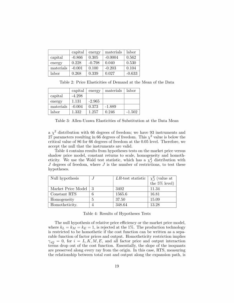
Tables 2 and 3 provide the mean price elasticities of demand and factorsubstitution elasticities.

The price elasticities have the expected signs. The substitution elas-ticities show all pairs of inputs to be substitutes except for materials andcapital, which show almost no complementarity. Given this, we can expectrelative price distortions to impact factor demand such that the demand forthose factors whose relative prices are lower than the rest to rise as producerssubstitute towards them. For instance, as the discussion in the next sectionshows, the relative price of materials to all factor inputs is distorted down-wards, and we expect the substitution towards materials to be exaggeratedas a result. This is what we do observe.

We have checked the properties of the shadow cost function to ensureit corresponds to a well-behaved cost function. Linear homogeneity holdssince it is imposed for estimation. For monotonicity, we look at the signs ofthe fitted factor share equations. These are all positive at all data points.For concavity, we examine the signs of the principal minors of the Hessianmatrix at the grand mean of the data. They have the expected alternatingsigns. The fitted cost function is also positive.

Our test of the overidentifying restrictions gives a value of 83 which has

10Further discussion of relative price efficiency appears in the following section.

17

Coefficient Parameter Estimates t-ratiosαo 1.025 14.69αQ 0.636 23.07αL 0.430 19.14αM 0.258 6.26αE 0.141 5.69αK 0.171 6.28δt 0.146 6.39γQQ 0.031 9.30γLQ -0.018 -8.53γMQ 0.012 4.54γEQ 0.013 7.80γKQ -0.007 -4.85γLL -0.023 -3.46γLM -0.034 -4.30γLE 0.029 6.19γLK 0.028 6.86γMM 0.074 4.42γME -0.018 -3.90γMK -0.022 -4.13γKK -0.0134 -1.26γKE 0.007 1.01γEE -0.018 -2.75kL 3.004 7.58kM 0.095 31.43kE 5.982 6.54TThe t-ratios for k0s are for the null thatthey are equal to 1.

Table 1: Parameter Estimates from the Shadow Model

18

capital energy materials laborcapital -0.866 0.305 -0.0004 0.562energy 0.228 -0.798 0.040 0.530materials -0.001 0.100 -0.203 0.104labor 0.268 0.339 0.027 -0.633

Table 2: Price Elasticities of Demand at the Mean of the Data

capital energy materials laborcapital -4.298energy 1.131 -2.965materials -0.004 0.373 -1.889labor 1.332 1.257 0.246 -1.502

Table 3: Allen-Uzawa Elasticities of Substitution at the Data Mean

a χ2 distribution with 66 degrees of freedom; we have 93 instruments and27 parameters resulting in 66 degrees of freedom. This χ2 value is below thecritical value of 86 for 66 degrees of freedom at the 0.05 level. Therefore, weaccept the null that the instruments are valid.

Table 4 contains results from hypotheses tests on the market price versusshadow price model, constant returns to scale, homogeneity and homoth-eticity. We use the Wald test statistic, which has a χ2J distribution withJ degrees of freedom, where J is the number of restrictions, to test thesehypotheses.

Null hypothesis J LR-test statistic χ2J (value atthe 5% level)

Market Price Model 3 3402 11.34Constant RTS 6 1565.6 16.81Homogeneity 5 37.50 15.09Homotheticity. 4 348.64 13.28

Table 4: Results of Hypotheses Tests

The null hypothesis of relative price efficiency or the market price model,where kL = kM = kE = 1, is rejected at the 1%. The production technologyis restricted to be homothetic if the cost function can be written as a sepa-rable function of factor prices and output. Homotheticity restriction impliesγiQ = 0, for i = L,K,M,E, and all factor price and output interactionterms drop out of the cost function. Essentially, the slope of the isoquantsare preserved along every ray from the origin. In this case, RTS, measuringthe relationship between total cost and output along the expansion path, is

19

unaffected by factor prices. The production technology is further restrictedto be homogeneous if RTS does not change as output increases. In thiscase, in addition to the homotheticity restrictions, the second order term inoutput is dropped: γQQ = 0. As a result, the average cost function doesnot change as output goes up, since total cost goes up by the same amountas output, and the average cost curve can not take a u-shaped form. Inaddition to the above restrictions, if γQ = 1, then we have constant returnsto scale. The test results in Table 2 show that we can reject homotheticity,homogeneity and constant returns to scale. Therefore, we retain all secondorder terms in the cost function and show their effect on returns to scalebelow.

5.2 Relative Price Efficiency, Cost and Factor Shares

As reported in Table 1, the shadow price factors indicate the existence ofrelative price inefficiency. These parameters can only be interpreted by theirrole in raising cost. Thus, for the normalization kK = 1, where we get kL =3.004, kM = 0.095 and kE = 5.98,these parameters indicate cost distortionsengendered by relative price inefficiencies. The first case, for instance, showsthat fL

fK= 3.004× PL

PK, and hence the marginal rate of technical substitution

between labor and capital that exceeds the market price ratio of these twoinputs; this is the Averch-Johnson (1962) type of effect. Similarly, the ratioof marginal products between energy and capital exceeds the ratio of theirmarket prices, while that between materials and capital falls below the ratioof their market prices. Such relative price inefficiencies raise cost above anefficient level that would prevail without the presence of distortions. Wediscuss the extent of these cost distortions below.

Since these parameter values are invariant to the choice of shadow pricefactor normalized, and the value given to it, they have further implicationsfor fi

fjbetween all pairs of inputs. Using the estimated values we obtain the

following:

fEfL= 1.991 fE

fK= 5.984 fE

fM= 63.62

fLfE= 0.502 fL

fK= 3.004 fL

fM= 31.95

fKfL= 0.330 fK

fE= 0.167 fK

fM= 10.64

fMfL= 0.030 fM

fK= 0.094 fM

fE= 0.020

Based on these, we find the relative shadow price of energy to shadowprices of all other factors to be highest, followed by the relative shadowprice of labor, then capital, and with the relative shadow price of materialsbeing the lowest. First, that the ratios of the marginal product of energyto the marginal product of all other inputs exceed the respective relative

20

market price ratios reveals the distortionary impact of energy price regula-tions. Essentially, domestic price ceilings on energy inputs lower the relativeprice of energy in the domestic market to that in the international market.At the prevailing relative price of energy, quantity demanded exceeds quan-tity supplied in the domestic market and the marginal product of energy isgreater than the observed market price. Therefore, the marginal productratios between energy and all other inputs exceed their relative price ratios.Second, the distortionary impact of labor market regulations lead to theratios of marginal product of labor to capital and materials to exceed theirrespective market price ratios. Third, the tax and import disincentives toinvestment result in the MRTS between capital and materials being greaterthan the ratio of their market prices.

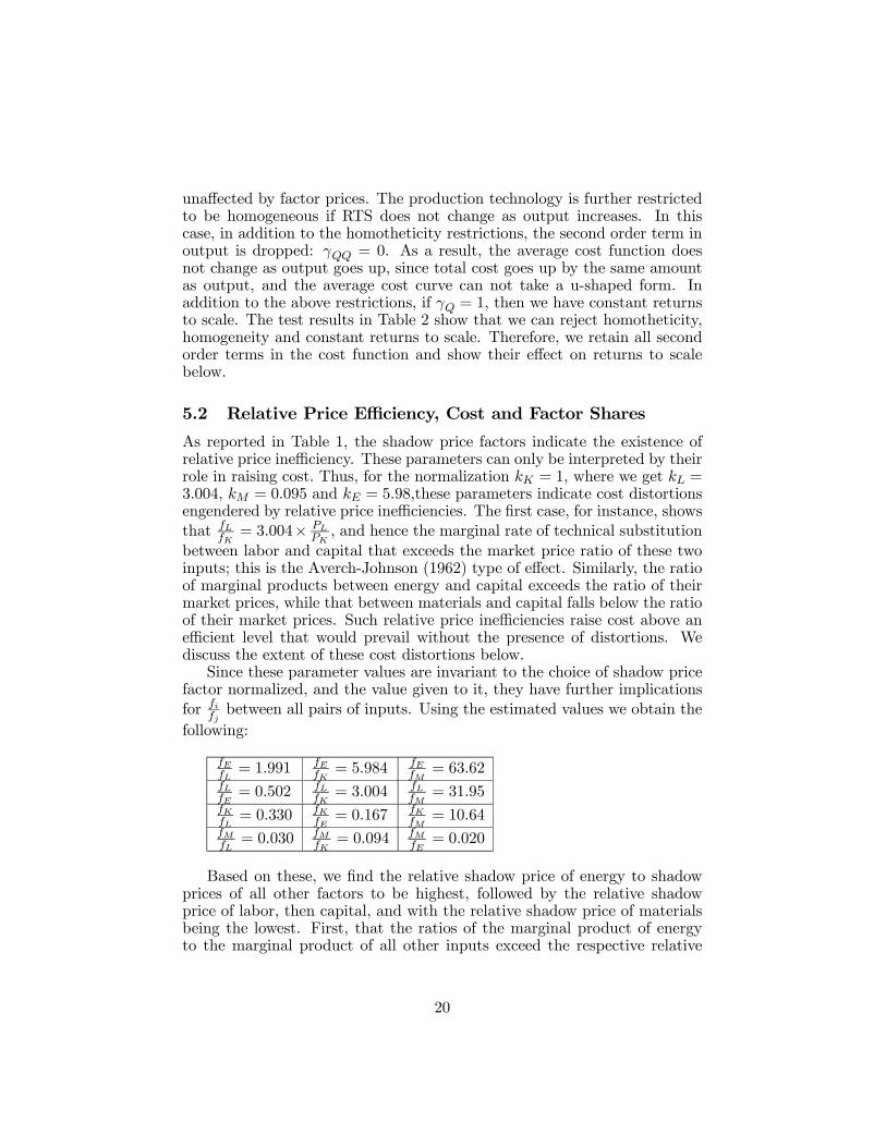
We study the effect of the regulatory constraints on actual or observedproduction cost and factor share usage by comparing fitted actual costsand shares under both relative price inefficiency and relative price efficiency.These values, at the data mean, are given in the first and second columns ofTable 5; the first column is based on the shadow price parameter estimatesunder relative price inefficiency while the second is based on shadow priceparameter estimates with relative price efficiency, kL = kM = kE = 1,imposed.

Actual values Actual values Shadow valueswith relative with relativeprice inefficiency price efficiency

Labor Share 9% 31% 42%Materials Share 75% 35% 11%Energy Share 3% 23% 27%Capital Share 13% 11% 20%Total Cost 511,610 LE 247,304 LE 335,738 LE

Table 5: Actual and Shadow Values of Total Cost and Factor Shares

Comparing the numbers in the first two columns, it is evident that theshare of labor and energy on average decrease with regulatory constraints,from 31% to 9% and from 23% to 3% respectively. On the other hand, theshare of materials increases significantly from 35% to 75% while that of cap-ital increases modestly from 11% to 13% under regulatory constraints. Theobserved cost, reflecting optimizing behavior based on observed or marketprices, is also double under regulatory constraints.

The more meaningful concept to consider, however, is the unobservedshadow cost, and the associated shares, which reflect optimizing behaviorincorporating the effect of the operating environment. In addition, thesevalues are what we need to focus on if we are interested in influencing firms’behavior by altering the institutional framework under which they operate.

21

Therefore, we focus on the results in the third column. They reflect thedecision of firms based on their perception of the effective cost of inputs; asstated earlier, the effective cost of energy is the highest, followed by that oflabor, then capital and last materials. These shadow share results suggestthat firms’ spending on factors whose effective prices are greater than isobserved is higher than is actually observed. Conversely, firms’ spending onthe factors they perceive as being relatively cheaper is less than is observed.The shadow cost share of materials is 11% while the observed share is 75%at the data mean. Therefore, private manufacturing firms’ spending onmaterials is less than is observed. On the other hand, the shadow cost shareof labor is significantly higher at 42% than the observed share at 9% at thedata mean as is the shadow cost share of energy at 27% than the observedshare at 3%. Similarly the shadow share of capital is higher at 20% thanthe observed share at 13%. This indicates that the effective cost shares ofenergy, labor and capital are higher than is observed.

Since we are interested in the impact of the reforms of the early 1990s,we carry out similar analysis by period; period one covers the years 1987-1990, and period two covers the years 1991-95. Table 6 presents the firstorder and shadow factor parameter estimates by period.

Period 1 Period 2Coefficient Estimates t-ratio Estimates t-ratioαo 1.484 4.01 1.754 2.38αQ 0.325 5.97 0.431 12.01αL 0.284 7.27 0.324 27.22αM 0.188 1.12 0.206 5.99αE 0.244 3.83 0.208 11.18αK 0.284 2.06 0.262 6.69δt 0.109 2.49 0.111 0.15kL 3.140 1.70 1.590 2.38kM 0.089 6.90 0.164 11.45kE 3.770 1.43 2.532 2.68The t-ratios for k0s are for the null thatthey are equal to 1.

Table 6: Parameter Estimates from the Shadow Model by Period

Once again the estimates of the shadow factors indicate the direction andmagnitudes of the relative price inefficiencies in the two periods. As before,the ratio of marginal products between energy and capital, and betweenlabor and capital exceed their market price ratios. The MRTS betweenmaterials and capital is similarly below this pair’s market price ratio. Mostimportantly, we observe the degree of distortions to be greater in period

22

Actual values Actual values Shadow values(inefficient) (efficient)

Period 1 Period 2 Period 1 Period 2 Period 1 Period 2Labor Share 7% 10% 31% 22% 34% 30%Materials Share 66% 71% 15% 35% 8% 21%Energy Share 5% 6% 24% 23% 26% 25%Capital Share 22% 13% 30% 20% 32% 24%Total Cost 226 LE 656 LE 102 LE 427 LE 155 LE 362 LETotal cost values in ’000s of Egyptian pounds

Table 7: Fitted Shares and Cost by Period

1 than in period 2. In particular, kL for period 1 is 3.14 while it is 1.58for period 2 and kE is 3.77 for period 1 while it is 2.53 for period 2. Theseindicate that although relative price inefficiency is not eliminated in period 2,the distortions in relative prices are lower in the second period. In addition,although kM is still significantly below 1 in period 2, at 0.16, it is closer toit than the period 1 value of 0.08.

Table 7 presents period one’s and period two’s fitted actual inefficient,efficient and shadow shares and cost values at the data mean.

We compare the effect of regulatory constraints on actual productioncost and factor shares in the two periods by looking at these values underrelative price inefficiency and efficiency. The direction of distortions are thesame in both periods, as indicated by the parameter estimates above, andmirror what we see for the entire period. However, the magnitudes of thesedistortions are lower in period 2 than in period 1. In particular, inefficientlabor share is below the efficient share by 24% in period 1 while it is so byonly 12% in period 2. Similarly, inefficient capital and energy shares arelower than their efficient counterparts by 8% and 19% respectively in period1 while they are so by 7% and 17% in period 2. Inefficient materials shareexceeds the efficient share by 51% in period 1 and by 36% in period 2. Theobserved cost under regulatory constraint is more than double in period 1while is higher by half as much in period 2. We also find similar resultswhen we compare shadow values with actual or observed values by period.

Tables 8 and 9 also present findings based on a similar approach for firmsclassified as medium versus large, by the number of workers they employ;medium firms employ 10 to 100 workers while large ones employ greaterthan 100 employees.

Relative price inefficiency is greater among large firms, where for exam-ple, kL = 3.428, compared to a value of 1.151 for medium firms. Therefore,on average, the effective or shadow share of labor in total cost is 31% whilethe observed share is 10% for larger firms. These figures are 20% and 6%for medium firms, which is a much smaller divergence. This result suggests

23

Medium Firms Large FirmsCofficient Estimates t-ratio Estimates t-ratiokL 1.151 1.62 3.428 6.20kM 0.164 21.40 0.105 11.1kE 2.42 3.90 4.605 6.30The t-ratios for k0s are for the null thatthey are equal to 1.

Table 8: Parameter Estimates from the Shadow Model by Firm Size

Actual Shadow Actual Shadowvalues values values values

Labor Share 6% 20% 10% 31%Materials Share 83% 40% 48% 5%Energy Share 2% 16% 8% 33%Capital Share 8% 24% 34% 31%

Table 9: Actual and Shadow Values by Firm Size

the input market constraints are more distortionary among ’labor-intensive’firms: As size here refers to the level of employment and not output. Re-duction in the distortionary constraints in the input markets, then, partlyexplains the higher productivity among labor-intensive sectors.

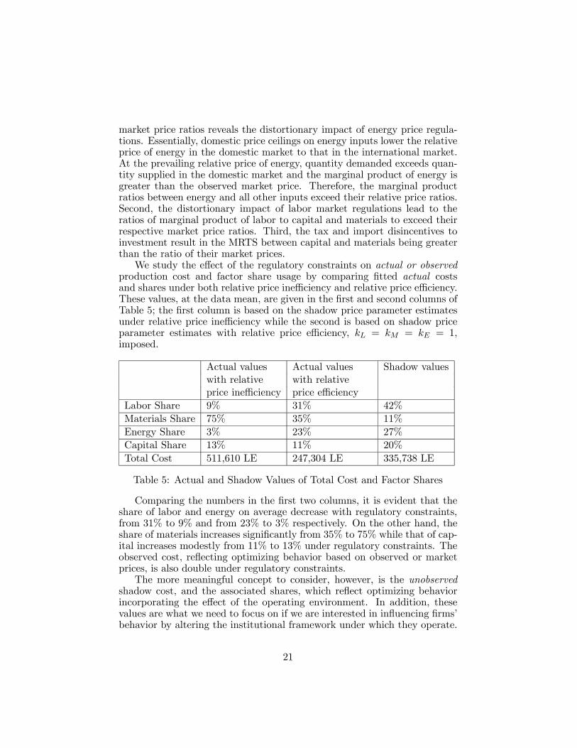
Overall, we can assess welfare loss by examining what value added11,employment and cost would be in the absence of inefficiencies engenderedby the operating environment. We examine the loss in value added by ob-taining fitted value added figures, output less materials, using fitted factorinput figures implied by both the efficient and inefficient cost models. Sim-ilarly, we examine employment by looking at both efficient and inefficientlabor demand. Table 10 presents the average efficient and inefficient labordemand, value added, shadow and total cost figures.

We can also examine welfare loss by looking at the above variables atall data points. Figure 3 presents shadow cost both in the presence ofdistortionary effects (CS) and in their absence (CSe) at all data points. Theshadow cost line under relative price inefficiency lies above the line obtainedby imposing relative price efficiency. This figure captures the extent of costdistortions that result due to inefficiencies in the operating environment.

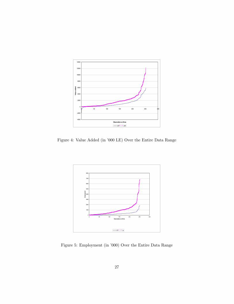
Figure 4 presents value added under comparable conditions: qvf repre-sents value added under the distortionary environment and qve representsvalue added in the absence of such distortions. As we expect, the value

11Value added is an output measure obtained by subtracting the materials quantitymeasure from the output quantity index.

24

Under Price Under Price PercentEfficiency Inefficiency Difference(in ’000 LE) (in ’000 LE)(or value) (or value)

Value Added 1901 975 95%Labor Demand 977 279 250%Shadow Cost 235 LE 316 LE 35%Total Cost 235 LE 494 LE 111%Cost values in ’000s of Egyptian pounds

Table 10: Welfare Loss (Average Values)

added line in the absence of distortion lies above the qvf line at all datapoints.

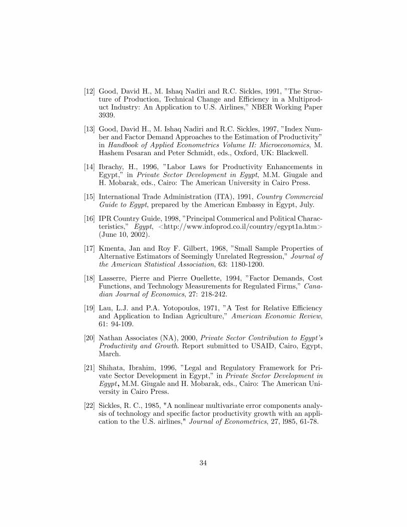
Figure 5 presents the employment situation under distortionary condi-tions (lF) and in the absence of distortions (le). Here again, we observethat labor demand would have been significantly higher if inefficiencies wereremoved.

Looking at similar welfare loss by period and firm size, we find the loss invalue added and employment, and total cost increases to be more magnifiedin period 1 and among large firms. Tables 11 and 12 provide the details atthe data mean.

Period 1 Period 2Under Price Under Price Percent Under Price Under Price PercentEfficiency Inefficiency Diff. Efficiency Inefficiency Diff.

Value Added 2192 1005 118% 2127 1211 76%Labor Demand 868 210 313% 766 358 114%Total Cost 104 LE 231 LE 119% 441 LE 682 LE 53%Values in ’000s of Egyptian pounds

Table 11: Welfare Loss by Period

5.3 Scale Economies

The relationship between total cost and output is measured by returns toscale (RTS), which is given by

∂ lnCA

∂ lnQ= αo+γQQ lnQ+

Xi

γiQ ln(kiPi)+

Pi γiQ(ki)

−1PiM

Si (ki)

−1 , i = 1...n (42)

25

0

500000

1000000

1500000

2000000

2500000

3000000

0 50 100 150 200 250 300

Observations on firms

Cos

t

CS CSe

Figure 3: Cost (in ’000 LE) Over the Entire Data Range

Medium Firms Large FirmsUnder Price Under Price Diffe- Under Price Under Price Diffe-Efficiency Inefficiency rence Efficiency Inefficiency rence

Value Added 1019 855 19% 2800 1796 56%Labor Demand 103 176 71% 1001 348 188%Total Cost 491 LE 592 LE 20% 184 LE 330 LE 80%Values in ’000s of Egyptian pounds

Table 12: Welfare Loss by Firm Size

for the actual cost function; we designate this ARTS. For the shadow costfunction, we delete the last term in (42) and designate it as SRTS.

We estimate ARTS and SRTS at all data points as well as at the grandmean of the data. Actual or observed RTS equals 0.95 while the shadowRTS equals 0.87 at the data mean. With relative price efficiency imposed,we find RTS to be 0.89. The ARTS of the inefficient model indicates that5% of the firms have constant or decreasing RTS while the SRTS indicatesthat all firms have increasing RTS. Similarly, the model with relative priceefficiency indicates all firms to have increasing RTS. We show these results atall data points for all three values by plotting scale economies (SE) againstoutput; SE = 1 − RTS. Figure 5 plots actual scale economies (ASE) andshadow scale economies (SSE) of the shadow price model against output,while Figure 6 plots SE of the relative price efficiency model against output.

The shadow price model’s SSE indicates that no firms have either de-

26

-4000

-2000

0

2000

4000

6000

8000

10000

12000

14000

0 50 100 150 200 250 300

Observation on firms

Valu

e ad

ded

qvf qve

Figure 4: Value Added (in ’000 LE) Over the Entire Data Range

0

1000

2000

3000

4000

5000

6000

7000

8000

0 50 100 150 200 250 300

Observations on firms

Empl

oym

ent

lF le

Figure 5: Employment (in ’000) Over the Entire Data Range

27

-0.05

0

0.05

0.1

0.15

0.2

0.25

0.3

0 5000 10000 15000 20000 25000

Output (in thousand LEs)

Scal

e Ec

onom

ies

SSE ASE

Figure 6: Scale Economies of the Inefficient Model Over the Entire OutputRange

0

0.05

0.1

0.15

0.2

0.25

0 5000 10000 15000 20000 25000

output (in thousand LEs)

Scal

e Ec

onom

ies

SE

Figure 7: Scale Economies of the Efficient Model Over the Entire OutputRange

28

creasing or constant RTS. Similarly, the relative price efficiency model’s SEmakes evident that all firms have increasing RTS. On the other hand, theshadow price model’s ASE shows that at the higher end of the output range,scale economies are constant or slightly negative. The behaviorally more rel-evant shadow price model indicates that all firms are not exploiting scaleeconomies. This is contrary to many empirical studies for different develop-ing countries that show the absence of unexploited scale economies amongbusiness firms, even small ones. Fikkert and Hansan (1998) find that the av-erage returns to scale is not significantly different from one for some industrygroups of the Indian manufacturing sector from 1976-1985; this is especiallyso for the largest firms. They also find, however, the presence of increasingreturns to scale for a large number of firms. Their study, which focuses onthe impact of regulation on returns to scale, leads them to conclude thatthe relaxation of the licensing regime, which inhibits firm expansion, maycontribute to gains in scale efficiency.12 Similarly in our study, the shadowprice model indicates that the Egyptian private manufacturing firms areoperating below the minimum efficient scale and reforms in the operatingenvironment are likely to have positive impact on scale efficiency.

Examination of RTS by period indicates that during period 1 actual RTSis 0.94, while it is 0.98 for period 2 at the data mean. On average, then,exploitation of SE has improved in period 2.

6 Concluding Remarks

The use of a generalized cost function allows us to study the impact of theoperating environment on the structure of production. Our general findingsindicate that the total costs of Egypt’s private manufacturing sector firmswere higher as a result of these constraints. The impact of the constraints hasbeen such that relative price distortions result in inefficient factor demandsthat increase total cost. In particular the contribution to cost increase ishighest from distortions in the energy input market, followed by those inthe labor and capital input markets. Our results also indicate that pricedistortions are greater among larger firms. Looking at the welfare loss en-gendered by these distortions, we see that for a labor abundant country likeEgypt, which has a high unemployment rate, correcting relative price dis-tortions is highly desirable; correcting such distortions will illicit the neededsupply response to enhance the economic output and employment needs ofthe sector. Generally, reforms appear to have had favorable impact on ef-fective cost and relative price inefficiency reductions, as indicated by firms’performance during the second period.

12They indicate in the Indian manufacturing sector, for the years covered, factors otherthan the licensing regime may be responsible for the inefficient scale of operations. Amongthese possibilites are the government’s control of financial enterprises which favor govern-ment enterprises in the allocation of credit and the condition of demand for firms’ output.

29

7 Appendix I

Private sector manufacturing data were obtained from the Central Agencyfor Public Mobilization and Statistics (CAPMAS) in Egypt from a pub-lication called Industrial Production Statistics. This publication is basedon data collected according to questionnaire No. 150. Normally data arecollected during fiscal year starting July 1st to June 30th for companiesfollowing this accounting system and calendar year for companies followingcalendar years.

The first industrial statistics survey was issued by CAPMAS with thegeneral census in 1937. Then industrial statistics were issued every 3 years:1944, 1947 and 1950. They were issued every 2 years from 1952 to 1956on establishments employing 10 workers or more. Starting from 1957, thesurvey was conducted annually on public enterprises, and starting from1964/65 both public and private enterprises were included in one document,in CAPMAS’ publication on industrial establishments employing 10 workersor more. Starting from 1989/90, publications were in separate documentsfor each public and private sector enterprises. Starting from 1991/92, an-nual industrial statistics were divided into the private formal, informal andinvestment sectors.

The private formal sector is governed by law 159 of 1981 concerningaudited accounting. It includes joint stock companies, limited by shares,limited liabilities, and branches of foreign firms. The informal sector consistsof companies not subject to law 159 of 1981 and investment law 230 of 1989and its amendments. It is made of partnerships, limited liabilities, de factocompanies, and single proprietorship. The investment sector includes thosethat are governed by investment law 43 of 1974, as amended by law 230of 1989 and law 8 of 1997 for investment incentives. The investment sectorincludes joint stock companies, limited by shares, limited liabilities, branchesof foreign companies, single proprietorship, partnerships and simple liabilityfirms.

Documents obtained cover a time series extending from 1986/87 to 1995/96,the last year available up to the time of this study, at the four-digit ISIC(International Standard Industrial Classification) level. From 1987/88 to1990/91, the data are aggregates of the private manufacturing sector ac-tivities of the whole republic. In other words, the inclusion of the formal,informal and investment private sector categories was not explicitly statedin CAPMAS publications for these years. However, it was later deducedfrom analysis conducted on the whole time series. From 1991/92 onwards,CAPMAS stated its publication of private manufacture sector activities intothese three separate categories.

Industrial data are arranged according to the three broad categories ofmining and quarrying, manufacturing and repair non-classified elsewhere.The current study is based on the manufacturing part of this industrialdata. The variables present in the data set include output at factor cost;

30

value added; taxes and duties; value of total revenues; total labor; totalwages, including basic salary, fringe benefits, and social insurance; total in-termediate materials, including local and imported raw materials, packingmaterials, fuel, electricity and spare parts; total intermediate services; cap-ital addition; fixed assets end of year; fixed assets depreciation; inventoryand change in inventory. Not all variables were available at the four-digitISIC level, particularly capital and investment data were only reported atthe three-digit level. Therefore, productivity estimation was based on three-digit ISIC level data.

Deflators used in the study are compiled from CAPMAS monthly whole-sale price indices covering the years 1972-1996. Capital goods deflators werealso available for the same years from CAPMAS. Energy deflators were cal-culated using energy prices facing the manufacturing sector over the periodunder study weighted by fuel mix used in the corresponding manufacturingactivities at the two-digit ISIC level.

We compute the output quantity index by dividing output at factorcost by the re-constructed wholesale price index. We construct the valuefor materials by subtracting the value of fuel and electricity from the totalintermediate goods and services. We then deflate this by the intermediategoods deflator provided by CAPMAS to get a materials index. We dividethe value of fuel and electricity by the energy deflator to obtain a quantityindex for energy. The energy deflators are a weighted-sum of energy pricesfaced by the manufacturing sectors for the period under study. The fuelmix used by each sector provides the weights. Using total wages and totallabor figures, we obtain the labor price by dividing the total wage bill bytotal labor. We normalize the wage rate so that 1987/88 prices are 100 andobtain a labor quantity index by dividing the values of labor, total wages,by this price index.

The construction of the capital quantity and price indices are more elabo-rate. Capital stock values were obtained by applying the perpetual inventorymethod: k(t) = (1− δ)k(t− 1)+ I(t) where k(t) is the capital stock at timet, k(t − 1) is the previous period’s value, I(t) is current investment, calledcapital addition by CAPMAS, and δ is the rate of depreciation of the capitalstock. We used a depreciation rate of 6.9% calculated on the assumptionof a 10-year geometrically declining depreciation rate. In order to calculatethe capital stock series, starting in 1987/88, we used the 1970/71 k-stock asa benchmark.

This measure of capital is deflated by the rental price of capital, P (T ).We use the following version of the rental price formulation

P (T ) =

µ1

1− u(T )

¶pI(T − 1)r(T ) + δpI(T − 1)+ pIc(T ) (43)

where u(T ) is the effective corporate tax rate at time T , r(T ) is the nominalinterest rate, pI(T ) is the capital goods deflator, δ is the depreciation rate of

31

the capital stock and c(T ) is the effective property tax rate. The terms reflectthe cost of capital, replacement and indirect taxes respectively. (Christensen& Joregenson, 1979). A study by the Egyptian Center for Economic Studiesgives the effective corporate tax rate as 27% for the manufacturing sector,which we use. The property tax rate is estimated to be 16% and includesrental, security and occupancy taxes.

32

References

[1] Atkinson, S.E. and R. Halvorsen, 1984, ”Parametric Efficiency Tests,Economies of Scale, and U.S. Electric Power Generation,” InternationalEconomic Review, 25: 64-662.

[2] Averch, Harvey and Leland L. Johnson, 1962, ”Behavior of the FirmUnder Regulatory Constraint,” The American Economic Review, 52:1052-1069.

[3] Barten, Anton P., 1969, ”Maximum Likelihood Estimation of a Com-plete System of Demand Equations,” European Economic Review, 1:7-73.

[4] Berndt, Ernst R., 1991, The Practice of Econometrics: Classic andContemporary, Reading, MA: Addison-Wesley.

[5] Bisat, Amer and Mahmoud A. El Gamal, 1999, ”Investment andGrowth in Egypt: 1970-1997: Lessons from the Past and Guidelinesfor the Future,” University of Wisconsin and IMF, memo.

[6] Brown, B.W. and M.B. Walker, 1995, ”Stochastic Specification in Ran-dom Production Models of Cost-Minimizing Firms,” Journal of Econo-metrics, 66 (1-2): 175-205.

[7] Christensen, Lauritis R. and Dale W. Jorgenson, 1969, ”The Measure-ment of U.S. Real Capital Input,” Review of Income and Wealth, 15:293-320.

[8] El Samalouty, Gannat, 1999, ”Corporate Tax and Investment Decisionsin Egypt,” Egyptian Center for Economic Studies Working Paper 35.

[9] Evanoff, Douglas D., Philip R. Israilevich and Randall C. Merris, 1990,”Relative Price Efficiency, Technical Change and Scale Economies forLarge Commercial Banks,” Journal of Regulatory Economics, 2: 281-298.

[10] Fikkert, B. and R. Hassan, 1998, ”Returns to Scale in a Highly Regu-lated Economy: Evidence from Indian Firms,” Journal of DevelopmentEconomics, 56: 51-79.

[11] Giugale, Marcelo M. and Hamed Mobarak, 1996, ”The Rationale forPrivate Sector Development in Egypt,” in Private Sector Developmentin Egypt, M.M. Giugale and H. Mobarak, eds., Cairo: The AmericanUniversity in Cairo Press.

33

[12] Good, David H., M. Ishaq Nadiri and R.C. Sickles, 1991, ”The Struc-ture of Production, Technical Change and Efficiency in a Multiprod-uct Industry: An Application to U.S. Airlines,” NBER Working Paper3939.

[13] Good, David H., M. Ishaq Nadiri and R.C. Sickles, 1997, ”Index Num-ber and Factor Demand Approaches to the Estimation of Productivity”in Handbook of Applied Econometrics Volume II: Microeconomics, M.Hashem Pesaran and Peter Schmidt, eds., Oxford, UK: Blackwell.

[14] Ibrachy, H., 1996, ”Labor Laws for Productivity Enhancements inEgypt,” in Private Sector Development in Egypt, M.M. Giugale andH. Mobarak, eds., Cairo: The American University in Cairo Press.

[15] International Trade Administration (ITA), 1991, Country CommercialGuide to Egypt, prepared by the American Embassy in Egypt, July.

[16] IPR Country Guide, 1998, ”Principal Commerical and Political Charac-teristics,” Egypt, <http://www.infoprod.co.il/country/egypt1a.htm>(June 10, 2002).

[17] Kmenta, Jan and Roy F. Gilbert, 1968, ”Small Sample Properties ofAlternative Estimators of Seemingly Unrelated Regression,” Journal ofthe American Statistical Association, 63: 1180-1200.

[18] Lasserre, Pierre and Pierre Ouellette, 1994, ”Factor Demands, CostFunctions, and Technology Measurements for Regulated Firms,” Cana-dian Journal of Economics, 27: 218-242.

[19] Lau, L.J. and P.A. Yotopoulos, 1971, ”A Test for Relative Efficiencyand Application to Indian Agriculture,” American Economic Review,61: 94-109.

[20] Nathan Associates (NA), 2000, Private Sector Contribution to Egypt’sProductivity and Growth. Report submitted to USAID, Cairo, Egypt,March.

[21] Shihata, Ibrahim, 1996, ”Legal and Regulatory Framework for Pri-vate Sector Development in Egypt,” in Private Sector Development inEgypt, M.M. Giugale and H. Mobarak, eds., Cairo: The American Uni-versity in Cairo Press.

[22] Sickles, R. C., 1985, "A nonlinear multivariate error components analy-sis of technology and specific factor productivity growth with an appli-cation to the U.S. airlines," Journal of Econometrics, 27, l985, 61-78.

34

[23] Sickles, R.C. and L. Getachew, 2000, ”An Analysis of Egypt’s PrivateManufacturing Productivity and Efficiency Growth,” in Nathan Asso-ciates (NA), Private Sector Contribution to Egypt’s Productivity andGrowth, Report submitted to USAID, Cairo, Egypt, March.

[24] Tybout, J.R., 2000, ”Manufacturing Firms in Developing Countries:How Well Do They Do and Why,? Journal of Economic Literature, 38:11-44.

35