1

The Real Option Approach to Adoption and Discontinuation of Management Accounting Innovation: The Case of Activity-Based Costing

Shu Feng1 Chun-Yu Ho

Department of Economics Department of Economics Boston University Boston University 270 Bay State Road 270 Bay State Road Boston, MA 02215 Boston, MA 02215 USA USA Tel: (857)-204-8979 Tel: (857)-204-0416 Fax: (617)-552-0431 Fax: (617)-552-0431 Email: fengshu@bu.edu Email: chunyu@bu.edu

1 Corresponding Author.

2

We would like to thank Alison Kirby Jones and Jianjun Miao for their helpful comments and suggestions.

3

The Real Option Approach to Adoption and Discontinuation of Management Accounting Innovation: The Case of Activity-Based Costing

Current Version: October 2005 Abstract This paper employs real option approach (ROA) to study the decision of ABC adoption and discontinuation under uncertainty. The general idea behind is that investing in ABC system is an option-rights as in financial American call option. The proposed model takes the total annual number of production of a firm as the primary decision variables. The added annual net profits after establishing ABC are considered in deciding the optimal threshold for adoption or discontinuation. Moreover, the difference between the ROA and the net present value (NPV) method is compared. We found that the optimal entry threshold for adoption obtained by the ROA is higher than that obtained by the NPV method. Conversely, the optimal exit threshold for discontinuation obtained by the ROA is less than that obtained by the NPV method. Thus, ROA is more conservative than the NPV method. The difference between these two methods is primarily driven by the option value of waiting before implementing the entry/exit project in the ROA.

Keywords: Activity based costing; Management accounting innovations; Real option theory; Investment under uncertainty

4

1. Introduction The activity-based costing (ABC) has been attracting widespread attention in the field of

management accounting. Cooper and Kaplan (1991) argue that ABC provides cost data

for improving production mix, process improvement, pricing and other managerial

decision. The ABC approach measures the costs of objects by first assigning resource

costs to the activities performed by the organization, and then using causal cost drivers to

assign activity costs to products, services, or customers that benefit from or create

demand for these activities. This approach captures the economics of the production

process more closely than traditional unit-based cost systems, which track the marginal

cost more closely than the unit cost. It reduces the difference between information

available to the firm and information required for decision making and hence to achieve

better decision and higher profitability.

The activity-based costing literature highlights three potential operational benefits: lower

costs, improved quality, and reduced manufacturing cycle time. First, as in Carolfi (1996),

ABC systems provide detailed information on the value-added and non-value-added

activities performed by the organization, the costs associated with these activities, and the

drivers of activity costs. This information allows managers to reduce costs by designing

products and processes that consume fewer activity resources, increasing the efficiency of

existing activities, eliminating activities that do not add value to customers, and

improving coordination with customers and suppliers. Moreover, Carolfi (1996) argue

that increased information about activities and cost drivers is also expected to enhance

quality improvement initiatives by identifying the activities caused by poor quality and

the drivers of these problems. As indicated in Cooper et al. (1992), ABC systems can

help justify investments in quality improvement activities that might otherwise be

considered uneconomic, and improve the allocation of resources to the highest valued

improvement projects by highlighting the costs of quality-related non-value-added

activities. Finally, many non-value-added activities such as counting, checking, and

moving increase the duration of a process or are driven by the amount of time a product

takes in an activity. By identifying activities that cause non-value-added time, Kaplan

5

(1992) argues that ABC can assist in justifying investments in cycle time reduction and

provide the detailed information needed to minimize delays.

Despite the vast literature2 in ABC, there is little discussion on the adoption of ABC.3 A

notable exception is Bjørnenak (1997) which conducts a survey which incorporating data

from 75 of the largest manufacturing companies in Norway. The results show that cost

structure is significant for ABC adoption. Companies have knowledge of ABC are more

likely to adopt the system. Also, it indicates a diffusion process that takes a contagious

form and points out the importance of institutional influence.

This paper contributes the literature by using real option approach4 (ROA) to study the

decision of ABC adoption under uncertainty. There are evidences that managers are using

ROA to evaluate project. According to Busby and Pitts (1997), they conducts a survey of

senior finance officers in the largest U.K. firms assessing how, in the absence of an easily

implementable normative model, firms think about real options during investment

appraisal. The results show that real options often occurred and were generally significant

in determining how decision-makers regarded an investment proposal. Graham and

Harvey (2001) survey a large representative set of US firms and find that a quarter of

them incorporate the real options of a project when evaluating it. Using the Dutch data,

2 The analytical studies focus on the use of ABC information for strategic decisions rather than for operational improvement. In contrast to claims by ABC proponents, analytical studies suggest that the cost data provided by ABC systems need not be more “accurate” than the costs reported by traditional unit-based systems. See Noreen (1991), Banker and Potter (1993), Datar and Gupta (1994), Christensen and Demski (1997), and Bromwich and Hong (1999). 3 There is a related literature on management accounting innovation. Dunk (1989) argue that lag in organizations may be due to the perceived greater complexity and lesser relative advantage, compatibility, trialability and observability of administrative (e.g., accounting) innovations as compared with technical innovations. Foster and Ward (1994) argue that perpetual accounting lag theory is derived from the organizational failure framework and markets and hierarchies theory. The theory asserts that operation of an internal labor market within a hierarchical organization inhibits management accounting innovation. 4 The real options studied in the literature include operating options in McDonald and Siegel (1985), the option to wait and undertake an investment later in McDonald and Siegel (1986) and uncertainty from future interest rates in Ingersoll and Ross (1992). On the empirical study, Pindyck and Solimano (1993) examine the relationship between uncertainty and investment. They use measures of economic and political instability to proxy for uncertainty about the marginal profitability of capital and inflation to proxy economic uncertainty. They find that inflation is inversely correlated with investment. Excellent surveys on real options and option pricing literature are provided by Amran and Kulatilaka (1999) and Broadie and Detemple (2004) respectively.

6

Verbeeten (2005) shows that the firm’s usages of sophisticated capital budgeting

practices include real option approach is increasing with the financial uncertainty and

firm size. Firms in financial services and building, construction and utility industry are

more incline to use complex capital budgeting practices.

The proposed model takes the total annual number of production of a firm as the primary

decision variables. The added annual net profits after establishing ABC are considered in

deciding the optimal threshold for adoption or discontinuation. Moreover, the difference

between the ROA and the net present value (NPV) method is compared. We found that

the optimal entry threshold for adoption obtained by the ROA is higher than that obtained

by the NPV method. Conversely, the optimal exit threshold for discontinuation obtained

by the ROA is less than that obtained by the NPV method. Thus, ROA is more

conservative than the NPV method. The difference between these two methods is

primarily driven by the option value of waiting before implementing the entry/exit project

in the ROA.

The general idea behind is that investing in ABC system is an option-rights. It can be

assimilated to the purchase of a financial American call option, where the investor pays a

premium price in order to get the right to buy an asset for some time at a predetermined

price (exercise price/strike price), and eventually different from the spot market price of

the asset (spot price). Analogously, the firm, in its investment decision, tries to get the

maximum firm’s current value of future discount payoff (a premium price), which gives

her the right to use the capital, the cost of setting up the ABC system (exercise price),

now or in the future, in return for the firm’s value worth a spot price. The value of the

option to adopt the ABC system is “An option on an option”, if we think of the firm’s

value as a derivative asset and take the profit flow as being the underlying asset. (In this

case the time horizon of the option is infinite). Taking into account this options-based

approach, the calculus of profitability cannot be done simply applying the net present

value rule to the expected future cash flows of the operation, but consider the following

three characteristics of the investment decision. First, there is uncertainty about future

payoffs from the investment. Second, the investment can be delayed. Third, the

7

investment is at least partially irreversible. The three characteristics imply that the

opportunity cost of investment includes the value of the option to wait that is

extinguished when an investment decision is taken. Therefore, the investment decision is

affected by the determinants of the value of this option and consequently, an appropriate

identification of the optimal exercise strategies for real options plays a crucial role in the

maximization of a firm’s value.

The article is organized as follows. Section 2 presents the model. Sensitivity analysis is

discussed in section 3. In section 4, numerical example is given in which we calibrate the

model to the data and then simulate it. Section 5 concludes and discusses the applicability

of the model to other management accounting innovation.

2. Model 2.1. Assumptions

ABC system provides more accurate information on cost for each product line. It enables

to the accounting number proxy the marginal cost more closely than the traditional unit-

based cost. Consequently, the firm can approach the profit maximization point closer than

before since it produces at a level closer to marginal cost equal to marginal revenue. If

the marginal cost is not accurate, it is difficult to get to that point by using the rough

information. Therefore, it is expected that the net profit after adopting ABC exceed that

from before. That is D – F ≥ 0 where D is average net profit after adopting ABC system,

which is average revenue minus average cost for each product. F is average net profit

from traditional unit-based cost system, which is average revenue minus average cost for

each product. Hence, the profit provides firms an incentive to establish ABC system.

However, the total demand of product produced by the firm fluctuates with the economic

environment. In the long term, the production is expected to grow owing to the economic

growth. Accordingly, this study assumes that the firm’s annual number of production, N,

follows a geometric Brownian motion (GBM). Consequently, the motions of N is

described as follows

8

N N NdN = dt + dzN

α σ (1)

The parameters αN and σN are the drift and volatility of N, respectively, and dzN denotes

the increment of a Wiener Process. From the above assumptions, a firm can increase net

profits after establishing ABC system. The added annual net profit π after using ABC is

= (D-F) N π (2)

By Ito’s Lemma (1951),

2

22

1d = dN + dN 2!N N

π ππ ∂ ∂∂ ∂

(3)

After some manipulation:

N N N N Nd = dt + dz dt + dzπ α σ α σπ

≡ (4)

where Nα α≡ . Eq. (4) shows that the stochastic process of π also follows a GBM with

drift α and volatilities σN.

2.2. Adoption decision

Generally, the investment project is worth assessing only when the added annual net

profit, π, from adopting ABC can break even or cross over the sum of initial investment

and maintenance cost of ABC. This model assumes that the ABC is completed TI years

after the initial investment decision is made. No cash flow, π, is produced during this

period. After the using of the ABC, we assume that a firm will spend C annually to

update and maintain the ABC operation forever. Assume this expense can support the

ABC system operating forever. Thus, the value of the project after ABC is established,

V1(π), can be obtained by

9

r

--r

](t)|ds C) - s) (t (e[)(0

rs-1

CEVαπππππ ==+= ∫

∞ (5)

where r is a specified discounted rate, which is the required rate of return for capital

investment. This study assumes r-α > 0, then the positive value of V1(π) holds.

When firm decides to invest in the system, it immediately incurs the setup cost I, which is

the initial invested capital to establish the ABC system. Moreover, this investment project

does not yield immediate cash flow during the period TI for setting up ABC system. τ

denotes the remaining time before ABC completion. The value of the project during the

ABC establishment period UI (π, τ) is obtained as follows

re-

-re](t)|) (t (E[e),(

-r)--(r

1r-

ττατ

απππτπτπ CVU ==+= (6)

The potential value of this project before investment, V0(π), is obtained by dynamic

programming with a specified discount rate r (Dixit and Pindyck, 1994). The value of the

project at time t can be expressed as the present value of its continuation value beyond

t+dt. That is

])(E[e)( 0-rdt

0 πππ dVV +=

Expanding the right-hand side using Ito’s Lemma, we have

)()1()(21)()( 0

''0

22'00 πππσπαππ VrdtdtVVV −++= (7)

and the volatility σ2 is defined as follows 2 2Nσ σ≡ . Simplifying, dividing by dt in Eq. (7),

the second order homogenous ordinary differential equation can be obtained

10

0)()()(21

0'

0''

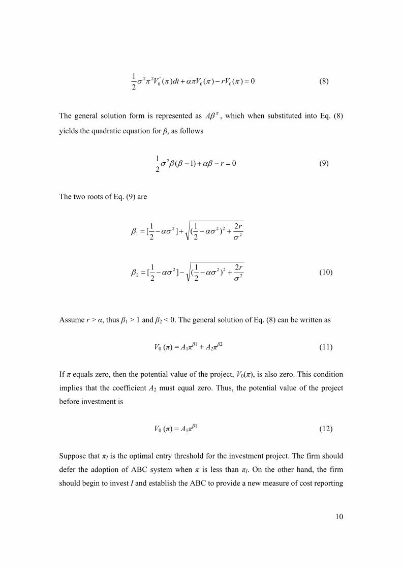
022 =−+ ππαπππσ rVVdtV (8)

The general solution form is represented as A πβ , which when substituted into Eq. (8)

yields the quadratic equation for β, as follows

0)1(21 2 =−+− rαβββσ (9)

The two roots of Eq. (9) are

2222

12)

21(]

21[

σασασβ r

+−+−=

2222

22)

21(]

21[

σασασβ r

+−−−= (10)

Assume r > α, thus β1 > 1 and β2 < 0. The general solution of Eq. (8) can be written as

V0 (π) = A1πβ1 + A2πβ2 (11)

If π equals zero, then the potential value of the project, V0(π), is also zero. This condition

implies that the coefficient A2 must equal zero. Thus, the potential value of the project

before investment is

V0 (π) = A1πβ1 (12)

Suppose that πI is the optimal entry threshold for the investment project. The firm should

defer the adoption of ABC system when π is less than πI. On the other hand, the firm

should begin to invest I and establish the ABC to provide a new measure of cost reporting

11

for managerial use when π increases to equal πI. Following the value matching and

smooth pasting conditions (see Dixit and Pindyck, 1994), we have

Value matching condition:

V0 (πI) + I = UI (πI, TI) (13)

Smooth pasting condition:

V0π (πI) = UIπ (πI, TI) (14)

Here, the smooth pasting condition ensures that πI is the entry threshold that maximizes

the potential value V0 (π) (Dixit, 1993). Substitute Eqs. (6) and (12) into Eqs. (13) and (14)

to solve the optimal entry threshold, πI, and the coefficient of the potential value, A1.

After some manipulations, we obtain

- -(r- )1

1

( ) [ e e ]1

I IT TI r r C rIα αβπ α

β= − +

− (15)

-(r- )1

1

1( ) e ITI IA rI αβπ α

β−

= − (16)

where TI is the period for establishing the ABC system. Substituting Eq. (3) into Eq. (15),

then the optimal entry threshold NI is obtained

- -(r- )

1

1

[ e e ]( )1

I IT TI

Ir C rIN

D F r D F

α απ β αβ

− += =

− − − (17)

In the NPV method, the NPV of a project is the sum of the present value of the expected

cash flow of the project and the salvage value at the end of the life of the project, minus

the initial investment cost. Typically, the NPV can be estimated at the time of decision-

making. The decision rule for the NPV method is described as follows. If NPV > 0, then

the investment project should be executed immediately, otherwise the project should be

12

abandoned. That is, the NPV method requires the present value of the expected cash flow

(π-C) after establishing ABC to exceed or equal the system setup cost, I. When the

following inequality is satisfied, the firm should invest in the project immediately.

( )( ) ( )0

0 1rt

tE t c e dt tπ π π

∞ − − = ≥ ∫ (18)

After some manipulations, we obtain the optimal entry threshold 0Iπ using the NPV

method.

( ) 110 r TTI

r Ce rIer

αααπ −−− = + (19)

Substituting Eq. (3) into Eq. (19) produces the optimal entry threshold 0IN using the NPV

Method

( ) 11

0 r TT

I

Ce rIerNr D F

ααα

−− +− =−

(20)

Comparing the optimal entry threshold obtained by the ROA, NI, in Eq. (17) with Eq. (20)

obtains the following result

01

1 1I IN Nββ

=−

(21)

The restriction on β1 > 1 leads to β1/(β1 -1) > 1, and thus the required optimal entry

threshold obtained by the ROA is higher than that obtained by the NPV method. The

difference between the two methods arises mainly because of the option value of waiting

before implementing the investment project. Since it considers the managerial flexibility

by including the option value in its calculations, the ROA method is more conservative

than the NPV method in supporting entry decision in the face of uncertainty. Thus, the

ROA is superior because it gives more accurate decision rule.

2.3. Discontinuation decision

If the added annual profit π from the ABC system cannot break even or cross over the

maintenance cost of ABC system, the ABC system adopted firm should consider

discontinuing the ABC system. We assume that the terminating project requires a period

TE to terminate the business completely and cash flow (π-C) will still occur during this

13

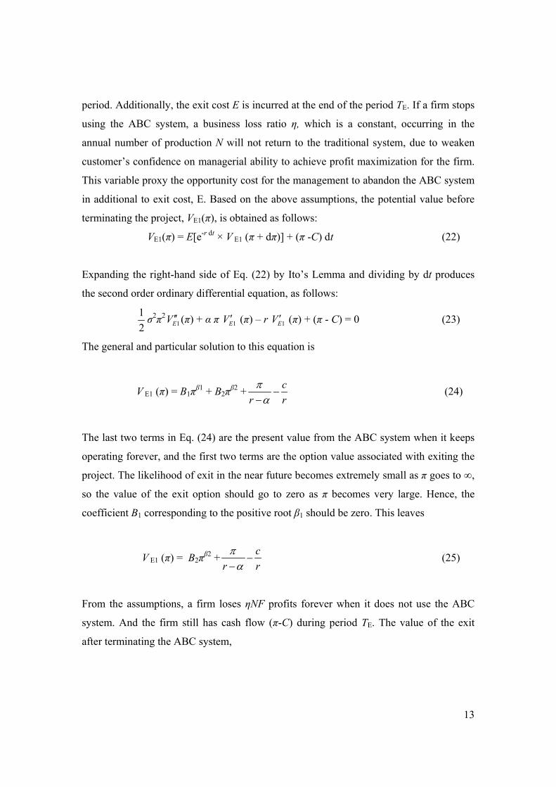
period. Additionally, the exit cost E is incurred at the end of the period TE. If a firm stops

using the ABC system, a business loss ratio η, which is a constant, occurring in the

annual number of production N will not return to the traditional system, due to weaken

customer’s confidence on managerial ability to achieve profit maximization for the firm.

This variable proxy the opportunity cost for the management to abandon the ABC system

in additional to exit cost, E. Based on the above assumptions, the potential value before

terminating the project, VE1(π), is obtained as follows:

VE1(π) = E[e-r dt × V E1 (π + dπ)] + (π -C) dt (22)

Expanding the right-hand side of Eq. (22) by Ito’s Lemma and dividing by dt produces

the second order ordinary differential equation, as follows:

12σ2π2

1EV ′′ (π) + α π 1EV ′ (π) – r 1EV ′ (π) + (π - C) = 0 (23)

The general and particular solution to this equation is

V E1 (π) = B1πβ1 + B2πβ2 + cr rπα−

− (24)

The last two terms in Eq. (24) are the present value from the ABC system when it keeps

operating forever, and the first two terms are the option value associated with exiting the

project. The likelihood of exit in the near future becomes extremely small as π goes to ∞,

so the value of the exit option should go to zero as π becomes very large. Hence, the

coefficient B1 corresponding to the positive root β1 should be zero. This leaves

V E1 (π) = B2πβ2 + cr rπα−

− (25)

From the assumptions, a firm loses ηNF profits forever when it does not use the ABC

system. And the firm still has cash flow (π-C) during period TE. The value of the exit

after terminating the ABC system,

14

V E0 (π) = ( )( )1 ( 1)E Er T rTF ce er D F r r

απ η πα α

− − − − −− − −

(26)

Denote τ as the time required to achieve a complete exit after deciding to terminate the

ABC system. The value of the exit project during the period TE, U2(π, τ), is obtained as

follows

U2(π, τ) = E[e-rτVE0(π(t + τ)) |π(t) = π] (27)

Substituting Eq. (25) into Eq. (26) obtains

U2 (π, τ) = ( ) ( )( ) ( )( ) ( )( )E Er T r r r T rF ce e e e er D F r r

α τ α τ α τ τ τπ η πα α

− − − − − − − −− − − −− − −

(28)

Suppose that πE is the optimal exit threshold for discontinuing the project. The firm

should continue to use the ABC system and defer the exit project when π is higher than

πE. On the other hand, the firm should begin to spend E and implement the exit project

immediately when π reduces to πE. Because the exit cost E is charged at the end of the

period TE, we obtain Eqs. (29) and (30) from value matching and smooth pasting

conditions.

Value matching condition:

U2(πE ,TE) + E · e-rTE = VE1(πE) (29)

Smooth pasting condition:

U2π(πE ,TE) = VE1π(πE) (30)

Substituting Eqs. (25) and (26) into Eqs. (29) and (30) to solve the optimal exit threshold,

πE, and the coefficient of the potential value B2, we obtain:

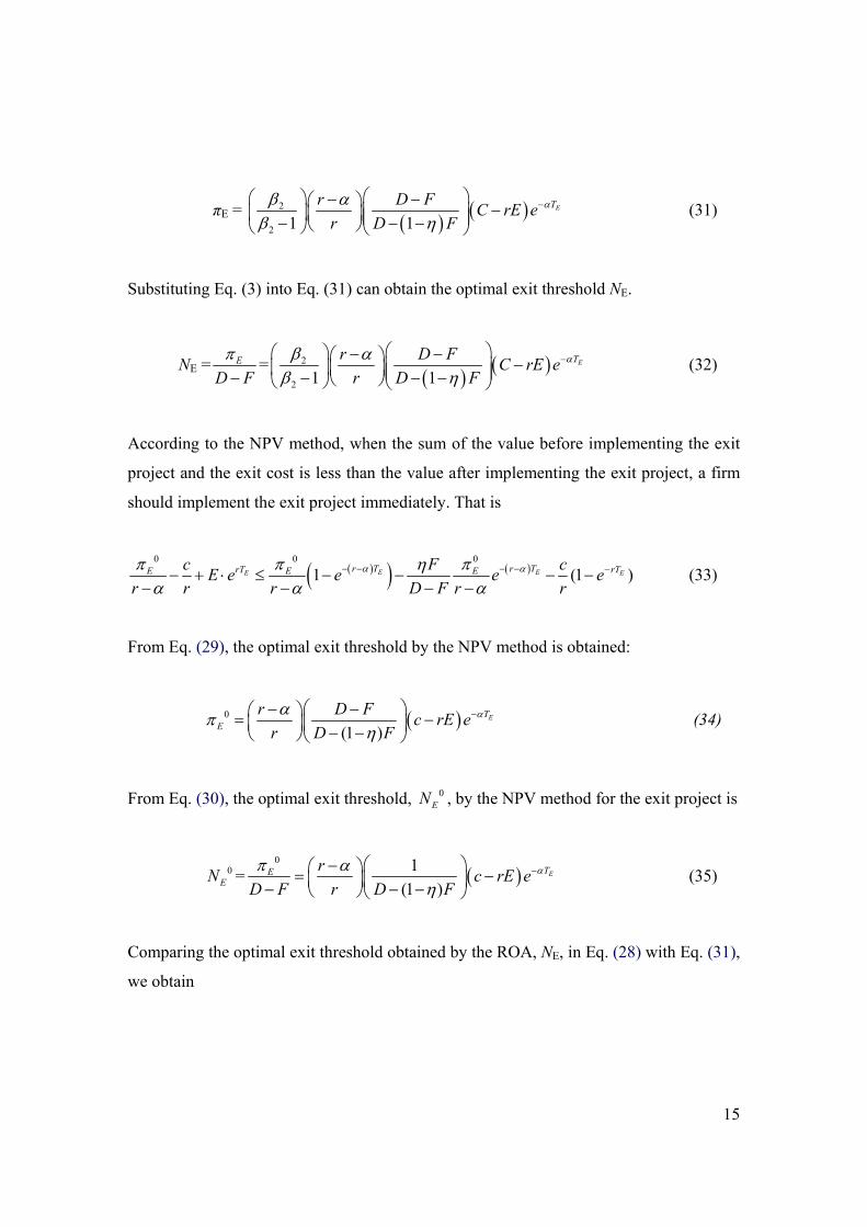
15

πE = ( ) ( )2

2 1 1ETr D F C rE e

r D Fαβ α

β η− − − − − − −

(31)

Substituting Eq. (3) into Eq. (31) can obtain the optimal exit threshold NE.

NE = E

D Fπ−

=( ) ( )2

2 1 1ETr D F C rE e

r D Fαβ α

β η− − − − − − −

(32)

According to the NPV method, when the sum of the value before implementing the exit

project and the exit cost is less than the value after implementing the exit project, a firm

should implement the exit project immediately. That is

( )( ) ( )0 0 0

1 (1 )E EE Er T r TrT rTE E Ec F cE e e e er r r D F r r

α απ π πηα α α

− − − − −− + ⋅ ≤ − − − −− − − −

(33)

From Eq. (29), the optimal exit threshold by the NPV method is obtained:

( )0

(1 )ET

Er D F c rE e

r D Fααπ

η− − − = − − −

(34)

From Eq. (30), the optimal exit threshold, 0EN , by the NPV method for the exit project is

0EN = ( )

0 1(1 )

ETE r c rE eD F r D F

απ αη

− − = − − − − (35)

Comparing the optimal exit threshold obtained by the ROA, NE, in Eq. (28) with Eq. (31),

we obtain

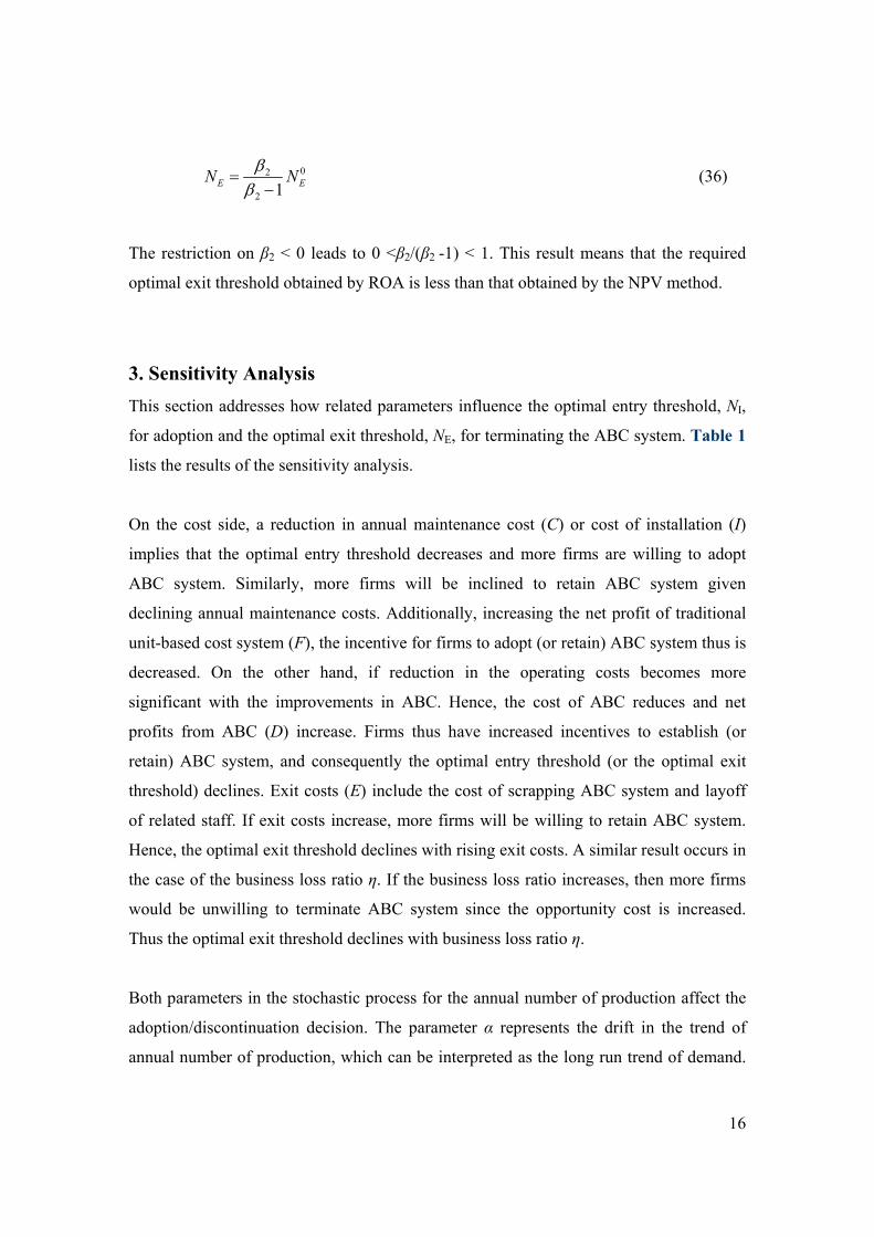
16

02

2 1E EN Nββ

=−

(36)

The restriction on β2 < 0 leads to 0 <β2/(β2 -1) < 1. This result means that the required

optimal exit threshold obtained by ROA is less than that obtained by the NPV method.

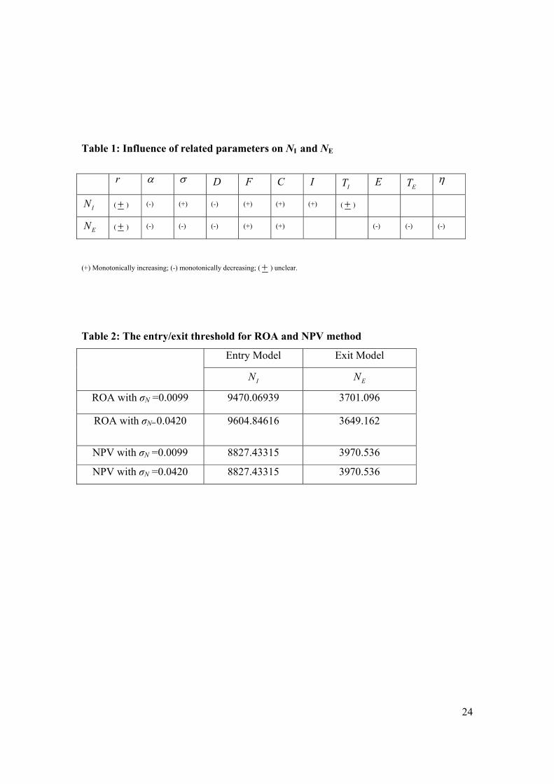
3. Sensitivity Analysis This section addresses how related parameters influence the optimal entry threshold, NI,

for adoption and the optimal exit threshold, NE, for terminating the ABC system. Table 1

lists the results of the sensitivity analysis.

On the cost side, a reduction in annual maintenance cost (C) or cost of installation (I)

implies that the optimal entry threshold decreases and more firms are willing to adopt

ABC system. Similarly, more firms will be inclined to retain ABC system given

declining annual maintenance costs. Additionally, increasing the net profit of traditional

unit-based cost system (F), the incentive for firms to adopt (or retain) ABC system thus is

decreased. On the other hand, if reduction in the operating costs becomes more

significant with the improvements in ABC. Hence, the cost of ABC reduces and net

profits from ABC (D) increase. Firms thus have increased incentives to establish (or

retain) ABC system, and consequently the optimal entry threshold (or the optimal exit

threshold) declines. Exit costs (E) include the cost of scrapping ABC system and layoff

of related staff. If exit costs increase, more firms will be willing to retain ABC system.

Hence, the optimal exit threshold declines with rising exit costs. A similar result occurs in

the case of the business loss ratio η. If the business loss ratio increases, then more firms

would be unwilling to terminate ABC system since the opportunity cost is increased.

Thus the optimal exit threshold declines with business loss ratio η.

Both parameters in the stochastic process for the annual number of production affect the

adoption/discontinuation decision. The parameter α represents the drift in the trend of

annual number of production, which can be interpreted as the long run trend of demand.

17

An increase in the trend makes the optimal entry threshold (and the optimal exit threshold)

decline, which implies that more firms would be willing to adopt (or retain) ABC system.

On the other hand, the entry and exit results for firm’s annual number of production

volatility (σ) differ. Increased volatility implies increased uncertainty of firm’s annual

number of production and firms require more time to obtain enough information for

making decisions on entering or retaining ABC system. This implies that firms will keep

holding the option and defer entering or exiting the ABC system. Increased volatility

decreases the incentive to adopt ABC system but increase the incentive to retain an

existing one. Therefore, an increase in the volatility increases the threshold of entry but

decreases the threshold of exit. It indicates that firms in growing and stable industries are

more likely to adopt the ABC system. Empirical test for this implication of the model is

left for the future research.

The relationship between threshold for entry/exit and discounted rate r is unclear. If the

discounted rate r increases, which makes the interest charge for entry/exit rise, more

firms would not be willing to adopt/terminate ABC system. Conversely, shorter period

for entry/exit reduces the interest charges for entry/exit, meaning more firms will be

willing to adopt/terminate ABC system. These two interactions simultaneously influence

the optimal entry/exit threshold. Thus, the relationship between the optimal entry/exit

threshold and discounted rate is unclear.

The effect of the time period for entry (TI) on the optimal entry threshold (NI) is also

unclear. The reasons are similar to the descriptions of the above paragraph for the

relationship between discounted rate and the optimal entry threshold. However, a rise in

the time period for exit (TE) decreases the optimal exit threshold. The relationship

between NE and TE differs from the relationship between NI and TI. Because the exit cost

E is charged at the end of time period TE, no interest charge rE exists during the exit

period. However, cash flow (π-C) still occurs during the exit period. Hence, more firms

would be willing to retain the ABC system if the exit time period increases.

18

4. Numerical Example This section simulates the adoption and discontinuation decision of ABC system for a

firm with the proposed model mentioned in the previous section. Numerical analysis is

conducted using the following parameters. Using 1929 to 2005 quarterly data of Real

GDP from Bureau of Economic Analysis, we get αN = 0.0084 and σN = 0.0099. Discount

rate is calibrated to r = 0.01 which is equal to average inflation adjusted return of U.S. T

Bills during the period 1929-2005. Hence, β1 = 14.74, and β2 =-13.74 are calculated from

Eq. (10). Since the setup cost is large relative to the maintenance and termination cost, we

assumes set up cost I, maintenance cost C, and exit lump-sum cost E and the average net

profit ABC system exceed the traditional unit- based cost system (D-F) have the ratio

relationship, E = C = 0.1*I, E/(D-F)= C/(D-F)=0.1*I/(D-F)=50000, in order to emphasis

the costs in the decision making process. Additionally, this investigation assumes that

the business loss ratio in N as η = 0.5, which implies (D-F)/[D-(1- η)F] = 2. It is the state

variable that we use to proxy the profitability of the firms. The time lags for entry and

exit project are TI = 0.5 years and TE = 0.5 years, respectively.

From these baseline parameters, the entry and exit thresholds for the decision of adopting

and discontinuing the ABC system are listed as Table 2. The drift parameter is at its

mean value and we take two level of volatility level around the mean to perform the

sensitivity analysis on the entry/exit threshold.

The numerical example illustrate that the entry threshold for adopting a new ABC system

is consistently higher for ROA approach than the NPV approach. It is due to the former

method incorporates the uncertainty of demand from output market into consideration.

The entry threshold from ROA approach is 7% - 8% higher that from NPV approach. The

entry threshold is increasing with the volatility parameter but the threshold from NPV

does not. On the other hand, the ROA provides a lower exit threshold than the NPV

method since it needs lower realization of output level in order to make the adopters give

up the ABC system. It is 7% - 9% lower than that from NPV approach. The exit threshold

is decreasing with the volatility parameter to show the waiting option is higher when

uncertainty is higher. Therefore, the ROA method is more conservative than the NPV

19

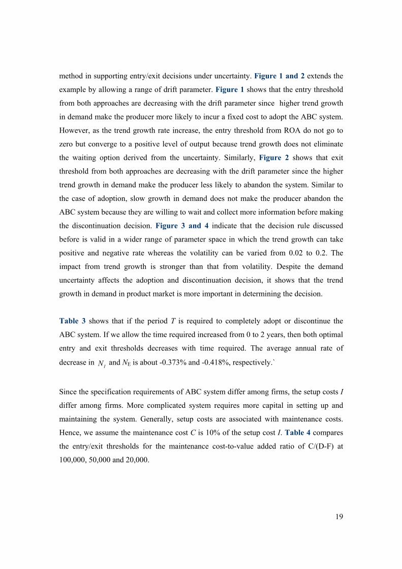
method in supporting entry/exit decisions under uncertainty. Figure 1 and 2 extends the

example by allowing a range of drift parameter. Figure 1 shows that the entry threshold

from both approaches are decreasing with the drift parameter since higher trend growth

in demand make the producer more likely to incur a fixed cost to adopt the ABC system.

However, as the trend growth rate increase, the entry threshold from ROA do not go to

zero but converge to a positive level of output because trend growth does not eliminate

the waiting option derived from the uncertainty. Similarly, Figure 2 shows that exit

threshold from both approaches are decreasing with the drift parameter since the higher

trend growth in demand make the producer less likely to abandon the system. Similar to

the case of adoption, slow growth in demand does not make the producer abandon the

ABC system because they are willing to wait and collect more information before making

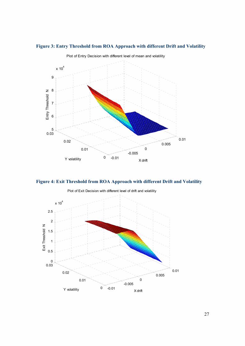
the discontinuation decision. Figure 3 and 4 indicate that the decision rule discussed

before is valid in a wider range of parameter space in which the trend growth can take

positive and negative rate whereas the volatility can be varied from 0.02 to 0.2. The

impact from trend growth is stronger than that from volatility. Despite the demand

uncertainty affects the adoption and discontinuation decision, it shows that the trend

growth in demand in product market is more important in determining the decision.

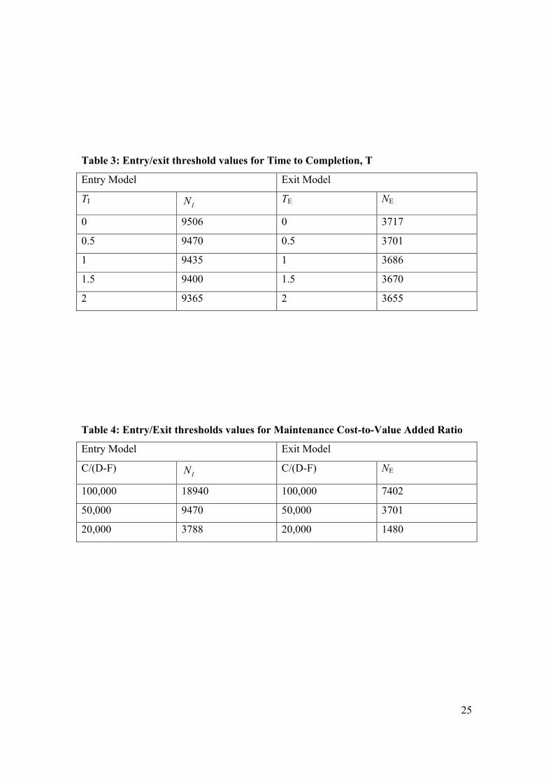
Table 3 shows that if the period T is required to completely adopt or discontinue the

ABC system. If we allow the time required increased from 0 to 2 years, then both optimal

entry and exit thresholds decreases with time required. The average annual rate of

decrease in IN and NE is about -0.373% and -0.418%, respectively.`

Since the specification requirements of ABC system differ among firms, the setup costs I

differ among firms. More complicated system requires more capital in setting up and

maintaining the system. Generally, setup costs are associated with maintenance costs.

Hence, we assume the maintenance cost C is 10% of the setup cost I. Table 4 compares

the entry/exit thresholds for the maintenance cost-to-value added ratio of C/(D-F) at

100,000, 50,000 and 20,000.

20

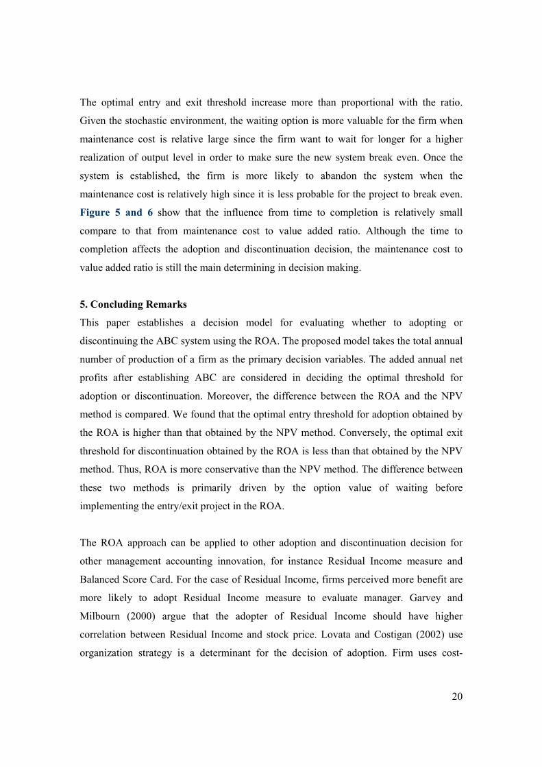
The optimal entry and exit threshold increase more than proportional with the ratio.

Given the stochastic environment, the waiting option is more valuable for the firm when

maintenance cost is relative large since the firm want to wait for longer for a higher

realization of output level in order to make sure the new system break even. Once the

system is established, the firm is more likely to abandon the system when the

maintenance cost is relatively high since it is less probable for the project to break even.

Figure 5 and 6 show that the influence from time to completion is relatively small

compare to that from maintenance cost to value added ratio. Although the time to

completion affects the adoption and discontinuation decision, the maintenance cost to

value added ratio is still the main determining in decision making.

5. Concluding Remarks

This paper establishes a decision model for evaluating whether to adopting or

discontinuing the ABC system using the ROA. The proposed model takes the total annual

number of production of a firm as the primary decision variables. The added annual net

profits after establishing ABC are considered in deciding the optimal threshold for

adoption or discontinuation. Moreover, the difference between the ROA and the NPV

method is compared. We found that the optimal entry threshold for adoption obtained by

the ROA is higher than that obtained by the NPV method. Conversely, the optimal exit

threshold for discontinuation obtained by the ROA is less than that obtained by the NPV

method. Thus, ROA is more conservative than the NPV method. The difference between

these two methods is primarily driven by the option value of waiting before

implementing the entry/exit project in the ROA.

The ROA approach can be applied to other adoption and discontinuation decision for

other management accounting innovation, for instance Residual Income measure and

Balanced Score Card. For the case of Residual Income, firms perceived more benefit are

more likely to adopt Residual Income measure to evaluate manager. Garvey and

Milbourn (2000) argue that the adopter of Residual Income should have higher

correlation between Residual Income and stock price. Lovata and Costigan (2002) use

organization strategy is a determinant for the decision of adoption. Firm uses cost-

21

leadership strategy is more likely to adopt Residual Income than those use differentiated

product strategy. However, the perceived benefit may not be realized once the new

measure is used. Lin (2005) investigate the discontinuation decision of firm on Residual

Income and find out that discontinuing firm experience less correction in investment, i.e

less realized benefit, than continuing firm. However, in the studies mentioned, there is no

consideration from the view of ROA approach. Exploring the implications from ROA can

deepen our understanding on the firm’s decision.

The model in this paper assesses the adoption and discontinuation decision separately.

When a firm considers adopting a new management accounting practice, it has an option

of adopting the practice, and also has the option of discontinuing the practice after having

using it. The current model can be extended to the case that a firm exercises an option to

adopt a new management accounting practice and own another option to discontinue the

practice and revert to the original practice. Therefore, two interlinked option pricing

problems must be solved simultaneously. Such an adoption and discontinuation decision

model for further research will provide a more thorough understanding on the life cycle

of management accounting practices.

References Amran, M. and N. Kulatilaka (1999) Real Options: Managing Strategic Investment in an Uncertain World. Boston, Harvard Business School Press. Anderson, S. W. and S. M. Young (1999) “The Impact of Contextual and Procedural Factors on the Evaluation of Activity Based Costing Systems,” Accounting, Organizations and Society, October: 525–59. Banker, R. D., and G. Potter (1993) “Economic Implications of Single Cost Driver Systems,” Journal of Management Accounting Research, Fall: 15–31. Bjørnenak, T. (1997) “Diffusion and accounting: the Case of Norway,” Management Accounting Research, 8 (1), 3–17. Bromwich, M., and C. Hong (1999) “Activity-Based Costing Systems and Incremental Costs,” Management Accounting Research, March: 39–60.

22

Broadie, M. and J.B. Detemple (2004) “Option Pricing: Valuation Models and Applications,” Management Science, September: 1145–1177. Busby, J. and C. Pitts (1997) “Real Options in Practice: An Exploratory Survey of How Finance Officers deal with Flexibility in Capital Appraisal,” Management Accounting Research, 8, 169–186. Carolfi, I. A. (1996) “ABM Can Improve Quality and Control Costs,” Cost & Management, May: 12–16. Christensen, J. and J. S. Demski (1997) “Product Costing in the Presence of Endogenous Subcost Functions,” Review of Accounting Studies, 65–87. Cooper, R. (1988) “The Rise of Activity-Based Costing-Part One: What is an Activity-Based Cost System?” Journal of Cost Management, Summer: 45–53. Cooper, R. and R. S. Kaplan (1991) The Design of Cost Management Systems, Englewood Cliffs, NJ: Prentice Hall. Cooper, R., R. S. Kaplan, L. Maisel, E. Morrissey and R. Oehm (1992) Moving From Analysis to Action: Implementing Activity-Based Management. Montvale, NJ: Institute of Management Accountants. Datar, S. M. and M. Gupta (1994) “Aggregation, Specification and Measurement Errors in Product Costing,” The Accounting Review, October: 567–91. Dixit, A. (1993) The art of smooth pasting. Gmbh: Harwood Academic Publishers. Dixit, A. and R. Pindyck (1994) Investment Under Uncertainty. Princeton University Press. Dunk, A. S. (1989) “Management Accounting Lag.” Abacus, September: 149–55. Graham, J.R. and C.R. Harvey (2001) “The Theory and Practice of Corporate Finance: Evidence from the Field,” Journal of Financial Economics, 60, 187-243. Garvey, G. and T. Milbourn (2000) “EVA versus Earnings: Does It Matter Which Is More Highly Correlated with Stock Returns?” Journal of Accounting Research, 38 (Supplement): 209-245. Ingersoll, J. and S.A. Ross (1992) “Waiting to Invest: Investment and Uncertainty,” Journal of Business, 65, 1-29. Lin, T. (2005) “Residual Income-based Compensation: Investment Activities and Discontinuation Decision,” National Chung Cheng University, mimeo.

23

Lovata, L. and M. Costigan (2002) “Empirical Analysis of Adopters of Economic Value Added,” Management Accounting Research, 13: 215-228. Ito, K. (1951) “On Stochastic Differential Equations,” Memoirs of American Mathematical Society, 1–51. Kaplan, R. S. (1992) “In Defense of Activity-Based Cost Management,” Management Accounting, November: 58–63. McDonald, R. and D. Siegel (1985) “Investment and the Valuation of Firms When There is an Option to Shut Down”, International Economic Review, 26, 331-349. McDonald, R. and D. Siegel (1986) “The Value of Waiting to Invest”, Quarterly Journal of Economics, 101, 707-727. Noreen, E. (1991) “Conditions Under Which Activity-Based Cost Systems Provide Relevant Costs,” Journal of Management Accounting Research, Fall: 159–68. Pindyck, R.S. and A. Solimano (1993) “Economic Instability and Aggregate Investment,” NBER Macroeconomics Annual, 8, 259-319. Verbeeten, F. (2005) “Do Organization Adopt Sophisticated Capital Budgeting Practices to deal with Uncertainty in the Investment Decision? A Research Note,” Management Accounting Research, 16: forthcoming.

24

Table 1: Influence of related parameters on NI and NE

(+) Monotonically increasing; (-) monotonically decreasing; (+ ) unclear.

Table 2: The entry/exit threshold for ROA and NPV method

Entry Model Exit Model

IN EN

ROA with σN =0.0099 9470.06939 3701.096

ROA with σN=0.0420

9604.84616 3649.162

NPV with σN =0.0099 8827.43315 3970.536

NPV with σN =0.0420 8827.43315 3970.536

r α σ D F C I IT E ET η

IN (+ ) (-) (+) (-) (+) (+) (+) (+ )

EN (+ ) (-) (-) (-) (+) (+) (-) (-) (-)

25

Table 3: Entry/exit threshold values for Time to Completion, T

Entry Model Exit Model

TI IN TE NE

0 9506 0 3717

0.5 9470 0.5 3701

1 9435 1 3686

1.5 9400 1.5 3670

2 9365 2 3655

Table 4: Entry/Exit thresholds values for Maintenance Cost-to-Value Added Ratio

Entry Model Exit Model

C/(D-F) IN C/(D-F) NE

100,000 18940 100,000 7402

50,000 9470 50,000 3701

20,000 3788 20,000 1480

26

Figure 1: Entry Threshold from ROA and NPV Approach

-4 -2 0 2 4 6 8 10

x 10-3

0

1

2

3

4

5

6

7

8

9x 104

X (alpha N=drift)

Y (E

ntry

thre

shol

d N

)

Plot of Entry Decision with different level of volatility

NPV with volatility=0.0099 and 0.0420ROA with volatility=0.0099ROA with volatility=0.0420

Figure 2: Exit Threshold from ROA and NPV Approach

-4 -2 0 2 4 6 8 10

x 10-3

0

1

2

3

4

5

6x 104

X (alpha N=drift)

Y (

Exi

t thr

esho

ld N

)

Plot of Exit Decision with different level of volatility

NPV with volatility=0.0099 and 0.0420ROA with volatility=0.0099ROA with volatility=0.0420

27

Figure 3: Entry Threshold from ROA Approach with different Drift and Volatility

-0.01-0.005

00.005

0.01

0

0.01

0.02

0.035

6

7

8

9

x 104

X drift

Plot of Entry Decision with different level of mean and volatility

Y volatility

Ent

ry T

hres

hold

N

Figure 4: Exit Threshold from ROA Approach with different Drift and Volatility

-0.01-0.005

00.005

0.01

0

0.01

0.02

0.030

0.5

1

1.5

2

2.5

x 104

X drift

Plot of Exit Decision with different level of drift and volatility

Y volatility

Exi

t Thr

esho

ld N

28

Figure 5: Entry Threshold from ROA Approach with different Maintenance Cost to

Value Added Ratio and Time to Completion

24

68

10

x 104

01

2

340

2

4

6

8

10

12

x 104

X Ratio C/(D-F)

Plot of Entry Decision with different level of ratio and time lags

Y time lags for entry

Ent

ry T

hres

hold

N

Figure 6: Exit Threshold from ROA Approach with different Maintenance Cost to

Value Added Ratio and Time to Completion

24

68

10

x 104

01

2

340

0.5

1

1.5

2

x 104

X Ratio C/(D-F)

Plot of Exit Decision with different level of ratio and time lags

Y time lags for exit

Exi

t Thr

esho

ld N