The Real Effects of Uncertainty on Merger Activity*

Vineet Bhagwata Robert Damb

Jarrad Harfordc

September 2015

Abstract

Deals for public targets take significant time to complete. During the interim, firm values can change substantially, inducing the parties to prefer deal renegotiation or termination. We predict the related costs will lead to increases in interim risk attenuating deal activity. We find increases in market volatility decrease subsequent deal activity, but only for public targets subject to an interim period. The effect is strongest when volatility is highest, for deals taking longer to close, and for larger targets. When possible firms appear to shorten the interim window as risk increases. Firm- and industry-level measures of uncertainty reveal similar findings, suggesting the effect is not simply driven by an unobserved macro-level variable. We conclude interim uncertainty is an important factor in understanding the timing and intensity of merger waves.

a Lundquist College of Business, University of Oregon b Leeds School of Business, University of Colorado at Boulder c Foster School of Business, University of Washington

                                                            * Correspondence to Robert Dam, University of Colorado, 202-903-6932, robert.dam@colorado.edu. The authors wish to thank Tim Burch, John Chalmers, David Denis (editor), Diane Del Guercio, Roberto Gutierrez, Karthik Krishnan, Katharina Lewellen, Micah Officer, Raghavendra Rau, two anonymous referees, and seminar participants at the Western Finance Association (2015), European Finance Association (2015), the University of Colorado, the University of Oregon and the University of Washington. Any errors are our own.

1

1. Introduction

The effect of uncertainty on investment has received growing attention in the literature

(see, for example, Bernanke (1983), Abel (1983), McDonald and Siegel (1986), Dixit and

Pindyck (1994) and Bloom (2007)). As we explain below, aspects of merger agreements yield a

direct channel for uncertainty to affect M&A investments, which are known to cluster in time

with pronounced peaks and troughs. Papers such as Mitchell and Mulherin (1996), Maksimovic

and Phillips (2001), Harford (2005), Ahern and Harford (2014) and others have focused on

economic, regulatory and technological shocks as well as macroeconomic conditions to explain

merger activity. Others, such as Shleifer and Vishny (2003), Rhodes-Kropf and Viswanathan

(2004) and Rhodes-Kropf, Robinson and Viswanathan (2005) have focused on explanations

driven by mispricing in the stock market. The general conclusion from the extant literature is that

there are many factors that contribute to the clustering of merger activity, but economic shocks

and macroeconomic conditions dominate.

In this study, we propose a new link between market conditions and merger activity.

Specifically, we predict that higher uncertainty will decrease deal activity. There are many

reasons why uncertainty may affect merger activity, but here we focus on its deal-specific effects

during the delay between deal announcement and completion. We begin by noting that the

Williams Act of 1968 (for tender offers) and proxy votes (for merger agreements) create a

material delay between the merger agreement and its consummation. With deals usually taking

over 90 days to complete, we estimate our sample targets experience an interim change in

standalone value of more than 10% almost two-thirds of the time, and greater than 20% over

one-half the time.

2

Such large changes should materially affect the appeal of the initial deal to both the target

and the bidder, thereby impacting their desire to complete the deal. Given that merger

renegotiations or terminations entail non-trivial costs to each party (Bates and Lemmon, 2003;

Officer, 2004), high volatility would make the marginal deal less profitable in expectation. In

addition, there is evidence to indicate that the bidder faces additional burdens during the interim

period as compared to the target. Namely, relevant Delaware case law hampers the bidder’s

ability to back out of the merger agreement, even if the target’s value changes substantially

(Gilson and Schwartz, 2005; Somogie, 2009). This produces the so-called “seller’s put,”

whereby the target can always put itself to the bidder at the bid price. While some of the interim

risk stemming from the “seller's put” could be contractible through the use of MACs (Gilson and

Schwartz, 2005; Denis and Macias, 2013), enforcing MACs requires litigation, entailing non-

trivial costs and risk for the parties involved. Further, Gilson and Schwartz (2005) and Denis and

Macias (2013) document that MACs generally assign industry and market-wide risks to the

bidder, implying a substantial portion of the interim risk is expressly borne by the bidder given

the target’s ability to find a better deal in favorable states.1

Regardless of the degree to which the interim risk is shared by the bidder and target, we

hypothesize that increases in overall economic uncertainty will lead to decreases in deal activity.

We test our hypothesis on a sample of mergers from 1990 to 2013. Using VIX as our proxy for

interim uncertainty, we find that a one standard deviation increase in VIX is associated with a

6% drop in public deal activity in the subsequent month. The effect is statistically significant,

and equates to a monthly decrease in deals of almost $4 billion.

                                                            1 In 2009, Dow Chemical attempted to back out of its deal to acquire Rohm & Haas Co., made in 2008 right before the global financial crisis hit credit markets as well as stock valuations. However, Rohm & Haas sued to force it to complete the deal noting, “You don’t get to renegotiate any contract you’re in just because you don’t like it anymore. Buyers often claim that, and it hardly ever works.” Dow quickly acquiesced and closed the merger on the original terms. (Pearson and Milford, 2009).

3

We test several additional hypotheses regarding the links between interim uncertainty and

merger activity. First, among the many factors affecting the timing of an acquisition, we expect

the interim risk will be a greater concern when volatility is higher, thereby increasing the

likelihood of significant interim changes driving ex post contract disputes. Sorting monthly deal

activity into quartiles by level of VIX, we find the effect to be insignificant in the lowest VIX

quartile, monotonically increasing in magnitude by quartile, and significant and double our

initially measured coefficient in the highest quartile.

Second, risk and its implied costs should be increasing in the time to completion. As a

result we expect the parties, to the extent legally feasible, to shorten the time-to-completion

window in response to increasing levels of VIX. If the interim risk is symmetric, both parties

would support a shortening of the interim window. If the risk is asymmetrically borne by the

bidder, lower bounds on acceptable bid premiums and court mandated maxima on break-up fees

would preclude bidders from offsetting the value of the option through other deal terms. In

tender offers, we observe a strong negative link between volatility and how long a tender is kept

open. A one standard deviation increase in VIX is associated with a 6 day shorter tender window,

relative to an average of 45 days. Regulatory scrutiny can create longer completion windows that

are beyond the parties’ control, and make these deals more sensitive to volatility changes. Deals

within concentrated industries are subject to the most scrutiny. Depending upon the specification,

we find that the effect of a change in VIX on deal activity in concentrated industries is double

that of non-concentrated deals, and generally only statistically significant in the former.

Third, we expect the size of the “position” in the implied option to affect the degree to

which it matters. Since the bidder is by definition taking a controlling interest in the target, we

use target size as a proxy for the size of the position. In deals for large public targets, the effect

4

of VIX on deal activity is over double that of the base effect and highly significant. For smaller

public targets, the effect is one-tenth of that in the larger deals and not statistically significant.

Underpinning all of these findings is the notion that macro-level uncertainty (VIX)

affects deals through its impact on deal-level interim uncertainty. To better confirm the link, and

also in an attempt to rule out some unobserved macro-level channel, we next explore the

relationship between volatility and acquisitions at the firm level. First, we examine the likelihood

that any particular firm becomes a target in a given year. We find that a firm is less likely to be a

target of an acquisition if its prior stock volatility is high. A one standard deviation increase in a

firm’s prior stock volatility is associated with a decrease in the probability of being a target from

4.5% to 2.9%. Additionally, when controlling for both firm and macro-volatility, only firm-level

volatility is significant, while macro-volatility’s incremental effect is not significantly correlated

with the likelihood of being a target. Furthermore, we find that a firm’s CAPM beta has a

negative association with a firm being a target, but the connection is driven by the subsample of

periods in which VIX is high. These findings support the hypothesis that macro-uncertainty

affects merger decisions through its firm-level effect on interim uncertainty.

We also repeat our other macro-level tests at the firm level and find similar results. When

split by size, the effect of volatility is negative and strongly significant for large firms but

actually positive and insignificant for small firms. Similarly, higher firm-level volatility leads to

shorter tender windows. Finally, we repeat the exercise at the industry level and again find a

strong negative relationship between measures of industry-level risk and industry-level deal

activity.

Of course, higher uncertainty also increases the value of waiting to exercise the “option

to merge” (Lambrecht, 2004; Morellec and Zhdanov, 2005), producing similar empirical

5

relationships between volatility and merger activity. Furthermore—despite the firm-level results

suggesting otherwise—there may be reasons to worry about an unobserved variable correlated

with VIX that affects deal activity. We address both cases by comparing public and private

firms. The law treats private targets (and subsidiaries of public targets) differently, such that it

should be easier for the firms to commit to deal terms, precluding ex post renegotiations and the

impact of interim risk.

We find that the previously observed relation between VIX and deal activity disappears

in our sample of private firms—the coefficient is one-tenth of that of public firms and

statistically insignificant. When we attempt to better match the two samples, we again find no

effect of VIX on deal activity in the private target market, regardless of the size of the target.

These results are consistent with—and help explain the findings of—Netter, Stegemoller and

Wintoki (2011), and Maksimovic, Phillips and Yang (2013), who both find that merger waves

are generally a public firm phenomenon but do not offer explanations as to why this would be

the case.

We provide further evidence inconsistent with competing hypotheses. In an attempt to

control for time-varying investment opportunities, we include year fixed effects in all of our

regressions. Alternatively, higher volatility might simply proxy for lower liquidity or higher

price levels, both of which are cited as affecting merger waves in the extant literature (Harford,

2005; Rhodes-Kropf et al., 2005; Edmans et al., 2012). However, we control for both effects in

our specifications and our findings are robust. Finally, this difference between public and private

targets is difficult to reconcile with any of these stories. Taking the results together, an

alternative explanation based on investment opportunities would need firm-level investment

opportunities to vary in a specific way over time that differs for private and public firms, large

6

and small firms, high and low beta firms, concentrated and unconcentrated industries and is

correlated with overall VIX. We know of no channel consistent with all of our findings other

than our interim risk hypothesis.

This interim risk channel assumes that renegotiations or terminations are sufficiently

common and costly to be a significant concern. We find that 16% of deals in our sample undergo

a renegotiation, while 22% actually end in termination. Additionally, we find that renegotiations

and terminations are statistically only more likely when doing so favors the target, consistent

with the seller’s put view of the interim risk. As a result, we attempt to value the implied put

option. We estimate the average put to be worth 6.5% of deal value in a tender offer and 11.1%

in mergers. Furthermore, the average month-to-month changes to the option value due to

volatility changes are 1.8% of deal value, while at the 75th percentile of volatility this number

jumps to 3.1% of deal value. The numbers suggest economically meaningful levels of both

interim risk and its variation over time.

If the risk is asymmetrically borne by the bidder, an obvious question is why the option

would not just be priced into the deal terms? Specifically, as interim risk increases, the parties

could increase the target termination fees and/or decrease the premium paid (Bhagwat and Dam,

2014). In both cases we find coefficients consistent with these predictions, but they are only

significant for bid premiums. However, when measured instead at the firm level as in Bhagwat

and Dam (2014), changes to target volatility have statistically significant effects on both. In

general, we find that while firms are adjusting deal terms to account for interim risk, they are

constrained enough so as to be unable to fully offset the effect of uncertainty on the value of the

seller’s put.

7

Our study contributes to the literature trying to understand the drivers of aggregate

merger activity. Prior research (Shleifer and Vishny, 2003; Rhodes-Kropf et al., 2005) has

attempted to explain waves of merger activity using aggregate price levels. We complement this

by showing that volatility has important implications as well. In doing so, we also contribute to

the larger literature on the effects of uncertainty on real investment, characterized by works such

as Bernanke (1983), Abel (1983), McDonald and Siegel (1986) Dixit and Pindyck (1994) and

Bloom (2007). Some of these papers deal with general uncertainty or policy uncertainty and

others deal with output price uncertainty in a real options framework. Here, we are investigating

a situation where a bidder commits to the investment (thereby providing the option), but has

uncertainty over both the completion of the deal and the value of the firm being acquired. In our

empirical setting, we are able to document that the elasticity of such investments to an increase

in uncertainty is negative and economically meaningful (approximately -0.3).

Furthermore, the interim risk channel provides a partial explanation for the difference in

merger wave behavior between public and private firms, previously documented but not fully

explained in Netter, Stegemoller and Wintoki (2011) and Maksimovic, Phillips and Yang (2013).

Finally, because regulation and court precedent are the channels through which uncertainty has

its effect, our study provides evidence of the real effects of legal constraints on the M&A market.

The study proceeds as follows. Section 2 reviews the literature and Section 3 describes

the data. We present the empirical results at the aggregate level in Section 4, and at the firm and

industry levels in Section 5. Section 6 provides some evidence regarding the frequency of

renegotiations and terminations, and attempts an estimation of the value of the implied option

therein. Section 7 discusses a number of robustness checks, with Section 8 offering concluding

remarks.

8

2. Literature Review

Early theoretical work on mergers and merger waves such as Coase (1937), Schumpeter

(1950), and Gort (1969) proposed heightened merger activity as a response to a shock (often

technological). Empirical studies focused on aggregate activity and on proving that it occurred in

waves or statistically distinguishable clusters (see, for example, Golbe and White (1988) and

Town (1992)). Mitchell and Mulherin (1996) show that aggregate merger waves are really

multiple simultaneous industry-level merger waves driven by industry-specific shocks.

Jovanovic and Rousseau (2002) establish that merger waves stretch back into the 19th century

and can be associated with technological shocks that increase dispersion in market-to-book

ratios. Shleifer and Vishny (2003), Rhodes-Kropf and Viswanathan (2004) and Rhodes-Kropf,

Robinson and Viswanathan (2005) explore rational and irrational links between stock market

valuations and merger waves. Harford (2005) shows that aggregate merger waves occur when

there is sufficient macro-level capital liquidity to allow industry-level shocks to propagate

waves, while Netter, Stegemoller and Wintoki (2011) and Maksimovic, Phillips and Yang (2013)

observe that the wave-like variation in merger activity is primarily found in the subset of public

firms. Duchin and Schmidt (2013) show that rational, efficiency increasing activity in merger

waves provides cover for increased agency-driven activity as well. Finally, Ahern and Harford

(2014) show that the trade flows between industries not only explain which firms merge, but also

how merger activity propagates through the economy along these trade flows. Their evidence

provides further explanation for how individual industry-level shocks can add-up to generate an

aggregate wave.

9

Notably, the extant literature has largely focused on efficiency, agency and behavioral

explanations and has linked merger wave activity to aggregate economic activity and stock

market valuations. Here, we focus on how uncertainty affects deal activity. Specifically, we

explore whether the legally mandated interim period is sufficiently costly or difficult to contract

around to the point where it has a real effect on merger activity.

The finance literature to date is largely lacking theoretical or empirical analysis of how

interim risk could affect aggregate merger activity. We propose that expected costs to either

party during the legally mandated interim period (such as renegotiation, litigation, or

overpayment, to name a few) should imply that higher expected uncertainty would make the

marginal deal less appealing, thereby have an ex-ante chilling effect on the number of announced

mergers. In addition, there is evidence to support the view that the bidder faces extra burdens in

altering or reneging on the original terms of the deal. This would imply that a merger agreement

is a put option given to the target by the bidding firm, thus further enhancing the effect of

uncertainty on deal activity.

The view of a merger agreement as a target put option originates in the legal literature.

Bainbridge (1990) highlights the risks created by the delay and suggests that the bidder bears

most of this risk. Fraidin and Hanson (1994) note that the contract in essence gives the target a

put option, in that its shareholders have the right but not the obligation to agree to the terms of

the deal. Gilson and Schwartz (2005) catalogue the rapid rise in contracts specifically excluding

adverse economic and industry outcomes from the material adverse effects (MAE) which would

allow the bidder to walk away. Regardless of the contract language, recent Delaware court cases

(IBP, Inc. v. Tyson Foods, Inc., 2001; Hexion Specialty Chemicals, Inc. v. Huntsman Corp.,

2008) at a minimum weaken the bidder’s ability to back out of deals, with Somogie (2009)

10

noting that the Delaware courts have never found a material adverse effect to have occurred in a

merger deal.

For most of our findings, the degree of symmetry in the interim risk does not matter: if

the interim risk has costly effects on either party, an increase in the risk should dampen deal

activity. While some of the findings here support the view that the risk is disproportionately

borne by the bidder (Bhagwat and Dam, 2015), we note that the two views are not mutually

exclusive.

3. Data

Our data for merger announcements come from Thomson One Securities Data

Corporation's (SDC) U.S. Mergers and Acquisitions database. We start with all merger

announcements in SDC between 1990 and 2013.2 After excluding all buybacks, share

repurchases, self-tenders, and spinoffs, we obtain data for 198,027 merger announcements, an

order of magnitude larger sample of merger announcements than most existing papers in the

literature (Netter et al., 2011).

We obtain data on the market expectations of volatility from the Chicago Board Options

Exchange (CBOE) website (http://www.cboe.com/micro/vix/historical.aspx). We use the closing

price of VIX on the last day of each month as our measure for the market expectations of

volatility over the next month.

                                                            2 We begin our sample period in 1990 because SDC coverage in the 1980s has been shown to be less complete than that since 1990 (Netter et al., 2011), and because the VIX data from the CBOE using the new methodology starts in 1990.

11

Since our goal is to link deal activity with market expectations of volatility, we measure

deal activity at a monthly frequency, as VIX is a 30-day forward looking measure of volatility

expectations. However, all our results are robust to using a quarterly frequency as well, where we

instead look at deal activity relative to VIX just prior to the quarter. For each month in the

sample, we tabulate the number of merger announcements for all targets, for public targets, and

for non-public targets (private targets and subsidiaries of either public or private targets). In

addition, we also calculate the percentage change in the number of announcements in each of the

three prior categories.

As a measure of price levels, we employ Robert Shiller’s Cyclically Adjusted Price

Earnings Ratio (CAPE) from his data website: http://www.econ.yale.edu/~shiller/data.htm. The

CAPE is defined as the current inflation-adjusted price level of the S&P 500 divided by the

simple average of the last 10 year’s inflation-adjusted earnings of the S&P 500. We obtain the

monthly return on the value-weighted stock market and calculate firm-level volatility with data

from CRSP, and use the spread between Aaa corporate bonds and the federal funds rates from

FRED as a measure of market-wide capital liquidity.3 For tender offers, we measure the length of

the tender window as the number of days from deal announcement to the initial tender date, as

reported by SDC. Finally, to measure the availability of internal funds, we also control for the

aggregate cash held by publicly traded firms, obtained from the most recent statements from

Compustat. Our primary sample consists of 286 monthly observations from March 1990 to

December 2013, inclusive.4

                                                            3We use the Moody’s Seasoned Aaa yield (http://research.stlouisfed.org/fred2/data/AAA.txt) for the monthly corporate bond yield and the Federal Funds rate, FEDFUNDS: http://research.stlouisfed.org/fred2/data/FEDFUNDS.txt. 4 Since the VIX price is a forecast of market volatility over the next 30 days, the first VIX forecast we use is the closing price on the last trading day in January 1990 as a proxy for market volatility for February 1990. In addition,

12

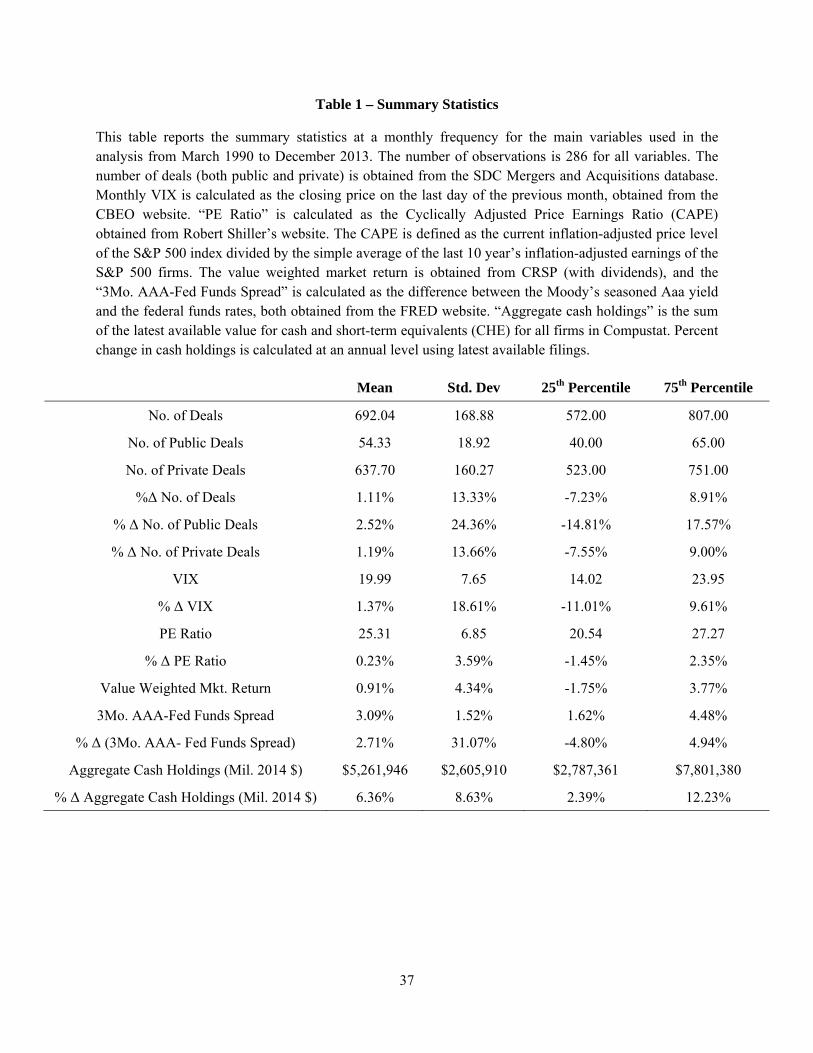
Table 1 presents summary statistics for the main variables used in our initial analysis.

The observations are at the monthly level. The first three rows summarize the number of deals.

The total number of deals averages 692 per month, of which 638 are private. Consistent with

prior work, we find that across public, private and total deals, there is significant variation in deal

intensity, as captured by the large standard deviations and inter-quartile ranges. Most of our

regressions are a percent-change regressed on a percent-change, so in the next three rows, we

present the percentage changes in each category of deal. VIX, our main variable of interest, has a

mean of 20 and an inter-quartile range of 14 to 24. We also transform it into percentage changes,

which shows similar variability. Finally, we present the summary statistics for the macro control

variables in our analysis: PE ratio, value-weighted market return, the AAA-Fed Funds spread,

and the amount of aggregate cash held by all publicly traded firms in Compustat. Note that the

aggregate cash variable is calculated using the latest available filings from Compustat and

percent changes in this variable are calculated at an annual level.

4. Interim Uncertainty and Aggregate Deal Activity

A. Merger Activity and Market Expectations of Volatility

Table 2 reports the results of a time-series OLS regression where the dependent variable

is the percentage change in the number of merger announcements with respect to the prior

month. All independent variables are constructed to include the information available before the

end of the prior month. That is, if the dependent variable is the percent change in merger

announcements from May to June 2000, all of our independent variables are percent changes in

                                                                                                                                                                                                the use of lagged changes in all our models implies we drop the first observation in the sample. Thus, our sample starts in March 1990, as opposed to January 1990.

13

their values from April to May 2000. The lone exception is the percent change in cash holdings,

which is calculated at an annual frequency using the latest available filings from Compustat.

The first panel estimates the regression over the sample of all merger announcements,

including public and private targets, and subsidiaries of public firms. Although there is a

negative association between percent change in VIX and the percent change in merger

announcements, it is not statistically significant, suggesting that volatility has little effect on

aggregate deal activity.

Panel B of Table 2 estimates the regression for the subsample involving public targets.

The first column of Panel B only includes a control for the percentage change in VIX in the

month prior to deal announcement. Even lacking other controls, the percent change in VIX is

negatively related to the subsequent percent change in merger announcements of public targets,

and has a t-stat of 1.38. Since both the independent and dependent variables are in terms of

percent changes, the coefficient can be interpreted as an elasticity. The elasticity of aggregate

merger activity with respect to market-wide expectations of volatility (VIX) is -0.11 when no

other controls are employed.

The addition of controls for market prices, stock returns, liquidity, and internal funds

increases the estimated elasticity of aggregate merger activity with respect to VIX to -0.29

(Column 2), while the significance increases to the 1% level. Column 3 further includes

indicators for each year and each calendar month, and clusters the standard errors at the year-

level. The point estimate is unchanged at -0.29, while the statistical significance drops to the 5%

level. To correct for any auto-correlation in the data, we employ Newey-West standard errors in

the last column (the correlation between contemporaneous and lagged residuals is -0.49 in Table

2). The auto-correlation is limited to a lag of 1, as the correlation between contemporaneous and

14

twice lagged residuals is -0.01. As shown in Column 4, the relationship between the percent

changes in VIX and merger activity remains negative and statistically significant at the 5% level.

The fact that the coefficient is unchanged in the presence of year and month fixed-effects helps

mitigate concerns that other omitted macro variables are correlated with the percentage change in

VIX, such as time-varying investment opportunities for example. As we discuss below, the fact

that we find the effect only in public deals, but not in private deals or deals for subsidiaries, is

consistent with our predictions, and is difficult to reconcile with investment and macro

conditions-based explanations.

The effect of increasing volatility on public acquisition activity is sizable: a one standard

deviation increase in VIX corresponds to a 6% decrease in the number of public deals, which

equates to a $4 billion monthly decline in merger activity (in inflation-adjusted dollars). In

robustness tests in Section 7, we confirm that these results hold at a longer (quarterly) frequency

as well.

We also note the results on two other control variables of interest. In contrast to Harford

(2005), we find no significant relation between deal activity and changes to capital liquidity,

although here we measure changes to liquidity rather than its levels.5 Furthermore, when

controlling for volatility we find that higher recent market returns are actually weakly associated

with lower levels of deal activity. This relation between market values and deal activity is quite

different from that documented elsewhere, where higher valuations and returns have been linked

to merger waves (Rhodes-Kropf et al., 2005; Edmans et al., 2012).

While we observe a strong negative relation between VIX and public firm deal activity,

no such relationship exists between VIX and deal announcements for private firms or                                                             5 In unreported tests, we compare the relation between the level of deal activity and the level of liquidity as measured by the spread, and find results regarding liquidity consistent with those reported in Harford (2005).

15

subsidiaries. As seen in Table 2, Panel C, in that subsample the coefficient on VIX is statistically

indistinguishable from zero. Moreover, the magnitude of the coefficient is over an order of

magnitude smaller than in the public target sample.

The difference in the relationship between VIX and deal activity for public versus private

targets is consistent with marginal public deals being delayed during times of high volatility due

to the increased costs of the interim risk (whereas private firms can ex ante commit to closing). It

does not appear consistent with an interpretation that higher volatility simply increases the value

of waiting (Lambrecht, 2004, Morellec and Zhdanov, 2005), as in this case the effect should be

felt on private targets as well. While we recognize that these two samples are inherently

different, it is notable that the effect of volatility on merger activity is only seen to be significant

for the set of public targets. This difference is also consistent with the results reported in Netter,

Stegemoller and Wintoki (2011) and Maksimovic, Phillips and Yang (2013), who find that the

waves in merger activity are largely confined to public firms. Although they posit some possible

drivers of this difference (differences in costs of restructuring, credit spreads, market valuations),

we offer results consistent with our hypothesis that interim risk contributes to the difference.

B. Variation in the Effect of Volatility on Deals

In Table 3, we test an extension of the hypothesis, specifically that a given increase in

VIX should matter more when price volatility is high, such that the risk involved is substantial.

We sort months into quartiles by end-of-prior-month VIX and re-estimate our specification from

Table 2. In the quartile of months with the lowest VIX, the coefficient on percent change in

volatility is actually positive but statistically insignificant. It is monotonically decreasing from

the lowest to the highest quartile, with the effect in the highest quartile almost double that

16

reported in Table 2, and significant again at the 5% level. The difference between highest and

lowest quartiles is also significant at the 5% level. These results suggest that the impact of price

volatility on merger activity is only present when volatility is high enough to make it an

important consideration. Measures of market returns and capital liquidity are again insignificant

across all quartiles. However, increases in aggregate cash holdings are associated with increases

in subsequent deal activity for the top quartile of VIX. These results are consistent with firms

tapping into their internal funds when external financing may be difficult to secure or when

speed of deal closure is paramount.

We note that when sorting months by VIX, a one percent change in VIX is inherently

different in the lowest quartile compared to the highest. Therefore, in columns 5 through 8 we re-

run the test controlling for the change in VIX rather than percent change. If anything, the results

are even more compelling in showing that the effect of a change in VIX is strongest during high-

volatility periods. 

 

C. Deal Completion Time

If the adverse effects of interim risk are increasing in volatility, a longer time to close

should increase the risk, and the expected costs therein, for any fixed volatility per unit time. We

first look at the relation between VIX and the length of the tender window, predicting that the

parties will agree to shorter windows (to the extent possible) when volatility is higher to

minimize the interim risk. Table 4 reports the results of an OLS regression where percent

changes to the length of the tender window is the dependent variable, and the main independent

variable of interest is again the prior percent change in VIX. We find a strong negative

correlation between the two, with an elasticity coefficient of -0.34, significant beyond the 5 or 1

17

percent levels depending upon the specification and controls. Relative to a mean tender window

of 45 days, a one standard deviation increase in VIX (38%) corresponds to a six day decrease in

the tender window (approximately a 1.5 standard deviation decrease).

Alternatively, in deals where the time to close is beyond the control of the firms, we

expect higher volatility to adversely affect the likelihood a deal can be reached ex ante. Due to

antitrust scrutiny, deals involving firms in concentrated industries should on average take longer

than deals involving firms in less concentrated industries. If so, higher volatility should have a

stronger attenuating effect on the former subset of deals.

An initial and brief Hart-Scott-Rodino (HSR) antitrust review is common for all but the

most competitive industries. If the industry is concentrated enough, the HSR review will take

considerably longer due to the so-called “second request” for information the government makes

of the merging parties. The proposed merger cannot be consummated until the parties have

complied with the government’s request for information and the merger has been cleared, which

would extend the time to completion and therefore the effect of volatility. While there is no

specific, codified review trigger, informal guidelines for triggering an HSR review refer to

industry HHI. As a rough proxy for deals that will likely get additional requests for information

and therefore take longer to close, we define a deal in which both the bidder and target belong to

an industry in the top two terciles of sales HHI concentration as a “concentrated merger”, and all

others as “non-concentrated mergers”.6 This corresponds to an HHI of 0.07 and higher for the set

of concentrated industries.7 We tabulate the percentage change in the number of merger

announcements for concentrated and unconcentrated industry targets in each month, and estimate

                                                            6 We employ the Fama-French 49 industry categorizations for this calculation. Results are robust to using the SIC classifications instead. Note that due to small sample concerns, we do not require the bidder and target to belong to the same industry. 7 The median industry HHI across all industry/years is 0.09 while the mean is 0.16.

18

our baseline regression separately for these two groups. We restrict our attention to deals

involving public targets since our earlier results indicate that uncertainty affects deal flow for

public and private targets differently. Deals in concentrated industries, as per our classification,

comprise 28% of all public deals and 31% of all deal value for public targets.

As shown in Table 5, the estimated effect of volatility on aggregate deal activity in the

concentrated industries is almost double that of the least concentrated, and is generally only

significant in concentrated industries. The difference in the coefficients between the two groups

is significant at the 5% level. This result, found across all specifications, is consistent with

standard option valuation theory, in which time to maturity interacts with volatility to increase

the value of the put. In the concentrated deals, we now see statistically significant impacts of

changes in liquidity, and the direction of the effect is consistent with that reported elsewhere in

the literature.

In order to include private firms in our analysis, we re-run the tests using industry

concentration ratios from the U.S. Census Bureau. The data are available going back to 1992,

and are updated every 5 years. We use the data from the most recent prior report to calculate the

percent of sales in each industry generated by its top 20 firms, and again consider a “high

concentration” deal to be one in which either the acquirer or target belongs to one of the top two

terciles of this ranking. While private firms are included in the Census Bureau data, not all

industries in Compustat are covered and, more importantly, the data is only available at five year

snapshots. Given the tradeoff between the two data sources, we only discuss the main results

here. The coefficient on concentrated deals is 2.5 times that in unconcentrated deals (-0.53 vs. -

0.19), and only significant in the concentrated deals. Furthermore, the difference between the

two is significant at the 5% level.

19

D. Effect of Target Size

Another major determinant of option value is the size of the underlying position. In our

scenario, this represents the size of the target, as the value of the option increases when the target

is larger. Furthermore, larger deals attract more antitrust scrutiny, simultaneously lengthening the

time to completion and increasing the value of the underlying option (as discussed in the

previous section). We thus explore the effect of deal size on the role of volatility in merger

activity, with the prediction that our results should be stronger in the subset of deals involving

large targets.

Another motivation for this test is that one major dimension on which public and private

targets differ is size. The average public target is much larger than the average private target. In

both cases, we therefore divide the sample into two groups, those deals that are worth less than

$250M (inflation adjusted to 2014 dollars) and those deals that are greater than $250M.8 This

breakdown should roughly match deals involving public and private targets on the one major

dimension on which they differ: size. We expect our results to be strongest for the subset of deals

involving large deals for publicly traded targets.

Some months lack observations involving large targets. Due to these few observations,

the percent change in the number of deals becomes highly volatile or is undefined in many

instances. For this reason, we aggregate deal activity at the quarterly level for this subsection.

                                                            8 Deal size is positively skewed: in 2014 dollars, the mean deal size is $339M, while the median is $32M. Roughly 80% of deals fall below the $250M cutoff. We use $250M as a cutoff to capture economically meaningful deals, not just ones that are large relative to the vast majority of small deals. Our results are robust to using alternate cutoffs of $75M and $150M. Similarly, our results are essentially unchanged when we right-hand censor deal values in an attempt to more closely match large public and private firms.

20

Note that all of our prior results are robust to using a quarterly frequency, as verified later in

Section 7.

We use the value of VIX just prior to the beginning of each quarter as a proxy of the

aggregate uncertainty for that quarter. We similarly obtain quarterly values for the market-wide

price-to-earnings ratio and value-weighted market returns. For a quarterly measure of capital

liquidity we calculate the spread between the 3 month maturity AAA bonds and Treasury bills,

obtained from FRED.

Panel A of Table 6 displays the results of a time-series OLS regression where the

dependent variable is the percent change in the aggregate deal announcements for each quarter,

restricted to the subsample of public deals and split by large and small deals. We find a small

positive, but statistically insignificant, effect of percent change in VIX on aggregate deal activity

for the subsample of deals involving small public targets. For public targets, the effect of

volatility on deal activity is concentrated in the larger deals. The elasticity of merger activity

with respect to VIX is -0.60 for large public targets, more than double the base effect

documented in Table 2 for all public targets. A 10% increase in VIX is associated with, on

average, 4 fewer large public mergers per quarter. Given that the average deal size of a large

public merger is $3.3 billion, this translates to a $13 billion decline in quarterly merger activity.

This effect is not only large economically, but also dwarfs the effects of volatility on the set of

small deals involving public targets and the set of deals involving any size range of private

targets. Moreover, this difference between the large and small public deals is statistically

significant at the 1% level. Note that large public deals, as we have defined them, comprise 51%

of all public deals and 96% of all deal value for public targets. They comprise 7% of deals for

either public or private targets, but over 53% of deal value over all deals during 1990-2013.

21

Panel B reports the results of a similar test, but estimated on the subsample of private

deals, split by deal size. For both large and small deals involving private targets, we generally

find a statistically insignificant effect of volatility on deal activity, except for weak significance

at the 10% level when the percent change in VIX is the only control for the sample of large,

private deals (Column 1 of the second set of results in Panel B). Therefore, regardless of the size

of the deal, VIX does not have any significant effect on private deal activity, consistent with the

lack of interim risk in deals for private targets and subsidiaries.

Combining the results in Panels A and B, we find a statistically significant effect of

percent change in VIX on aggregate deal activity only for the subsample of deals involving

larger public firms. This is consistent with the prediction that the value at risk must be

economically meaningful in order for volatility to impact the marginal deal. It is only for the

large, publicly traded targets where we find our main dampening effect of an increase in VIX on

aggregate deal activity. However, these deals represent the majority of deal value, so that the

overall effect is still economically significant.

5. Firm and Industry-Level Effects of Interim Uncertainty

A. Firm-Level Relationship Between Volatility and Merger Activity

All of the evidence presented thus far is consistent with the interim risk having a negative

effect on merger activity. The tests suggest that as overall market uncertainty increases, the

interim risk of the average target increases. In this section we turn our attention to firm-level

(and then industry-level) measures of both uncertainty and deal activity. We do this both to

control for the possibility of some unobserved channel between macro-level risk and deal

22

activity, and also to more closely link firm-level decisions to firm-level measures of interim

uncertainty. We also verify industry-level results are consistent with the market and firm-level

effects.

If the changes in deal activity are primarily being driven by interim deal uncertainty, we offer

the following two additional predictions. First, if both VIX and target volatility are measured

simultaneously, we expect the target volatility to have the larger effect. If instead VIX dominates

in predicting deal activity, we might suspect some unobserved macro-level channel unrelated to

the effect on the target firm’s price volatility. Second, because the relationship between firm

volatility and market volatility is increasing in the firm’s CAPM beta, we expect the effect of

VIX on the probability of a firm being a merger target to be strongest for high-beta firms during

episodes of high market volatility.9 At least theoretically, a high beta is irrelevant if there is no

market volatility. Similarly, high market volatility should have no effect on a zero beta firm.

Thus, results consistent with these predictions would be further evidence that macro-level

uncertainty impacts deal flow through its effect on target stock price uncertainty, and hence the

value of the seller’s put.

To test both predictions, we employ a logit model in which the dependent variable equals 1 if

a public firm becomes a target in a given year, and 0 otherwise. On average, 4.50% of firms are

the target of a merger or acquisition in a given year. Our sample now consists of 77,213 firm-

year observations from the CRSP-Compustat universe, with the merger events again taken from

the SDC U.S. Mergers and Acquisitions database. We include numerous firm-level explanatory

variables that also could affect the likelihood of a firm receiving an offer.

                                                            9 From the CAPM model, the variance of the firm’s returns is increasing in the variance of the market’s returns by a factor of beta squared. However, since less than 1% of our estimated betas are negative, for simplicity we use the CAPM beta as our measure, not beta squared.

23

We test our first prediction by comparing the relation between the likelihood a firm becomes

a target and both market-level and firm-level measures of volatility. For market volatility, we use

the VIX observation from the month before the year in question. For firm-level volatility, we

calculate the standard deviation of firm daily returns across the [t-13, t-2] months prior to the

year in question. We drop the t-1 observations to avoid any mechanical connections between

firm return volatility and rumors of an impending offer.

The first three columns of Table 7 present the results of this test. We see that at the firm

level, the point estimate on VIX is negative but near zero and statistically insignificant (Column

1). The coefficient on firm volatility is also negative, but is over an order of magnitude greater,

and significant at the 1% level (Column 2). When we control for both simultaneously (Column

3), the point estimates and significances are virtually unchanged. A one standard deviation

increase in a firm’s prior stock volatility is associated with a decrease in the probability of being

a target from 4.5% to 2.9%. Thus the effect of uncertainty on merger activity is primarily driven

by the effect of aggregate uncertainty on firm-level volatility, consistent with the implied put

option and not with an unobserved macro-level effect that is different from or incremental to the

effect of macro uncertainty on firm-level volatility.

For the second firm-level prediction, we measure a firm’s CAPM beta using daily returns

over months [t-13, t-2], using the Fama-French market factor as the benchmark. Additionally, we

split years into low- and high-VIX periods using the time-series median value. The results from

column 4 of Table 6 indicate that a firm’s market exposure, captured by the CAPM beta, is

negatively associated with the likelihood of the firm being a target. However, there is no

association between high levels of VIX and the likelihood of being a target (Column 5). When

we interact the indicator for periods of high VIX and a firm’s CAPM beta (Column 6), we find

24

that neither a high beta nor high market volatility alone impacts the likelihood of being a target.

However, the interaction between the two is negative and significant at the 5% level, suggesting

that high VIX only adversely affects firms with high levels of systematic risk, again supporting a

firm-level channel through which macro-volatility is affecting deal activity.

Finally, we repeat our previous tests on time to close and firm size at the firm level. Table 8

presents the results of OLS regressions looking at the tender window related to prior firm

volatility and the previous controls, we find that a one standard deviation increase in volatility

corresponds to a tender window that is three days shorter (again relative to a mean of 45 days),

significant at the 5% level.

Table 9 shows the link between volatility and deal activity at the firm level and split by firm

size. We see that for large firms the effect of volatility is still negative and significant at the 1%

level, while for small firms the point estimate is actually positive but statistically insignificant.

For large firms, we also again see that the negative link between VIX and becoming a target is

driven by higher beta firms during times of high market uncertainty.

B. Industry-Level Analysis of Interim Risk

As a final test of the link between changes in uncertainty and observed deal activity, we

repeat our tests at the industry level. Industries differ by deal level and volatility, so assessing the

effect at the industry-level can provide confirming evidence for our aggregate effect. Table 10

reports the results of OLS regressions where the dependent variable is the monthly percent

change in the number of deals at the industry level. We define industries using the Fama-French

17-industry classification. In addition to the previous explanatory variables, we calculate the

percent change in monthly volatility (by industry) using industry value-weighted daily returns.

25

In the first four columns, we report the results for public targets. Depending on the

specification, a one-standard deviation increase in industry-level volatility in the month prior

leads to a one-half standard deviation decrease in the subsequent number of deals, which equates

to a 1.7 percent decrease in observed deals. While industry volatility is negative and significant,

we see that the point estimate on VIX is not statistically significant, although the point estimate

is generally negative.

In columns 5 through 8 we repeat the regression on the sample of private deals, again at the

industry level. For private deals, neither the observed industry volatility nor VIX are statistically

connected to deal activity.

In robustness tests in Section 7, we verify our results hold when using deal value in dollars

rather than the number of years.

6. Economic Significance and Asymmetry of the Interim Risk

The results of Sections 4 and 5 are consistent with interim risk affecting deal activity for

public targets. However, they are consistent with both symmetric (Houston and Ryngaert, 1997;

Officer, 2004) and asymmetric (Gilson and Schwartz, 2005) views of the interim risk. In this

section we explore the degree to which the risk appears to be disproportionally borne by the

bidder or target. We also provide information on the frequency of renegotiations and

terminations, in support of the idea that the interim risk is a first-order concern, and that the

parties are responding accordingly when possible. Finally, we try to provide baseline estimates

of the value of the implied options and how much those values might change from month to

month.

26

A. Renegotiations—Frequency and Asymmetry

We begin by examining observed renegotiations and terminations. For interim risk to be of

material concern, we would expect ex-post alterations to be sufficiently common to warrant

attention. Furthermore, the states in which they are observed tell us something about the nature

of the risk. If large interim changes to either party’s standalone value in either direction lead to

similar incidences of deals being altered or cancelled, we would interpret this as being consistent

with both firms facing comparable interim risks. However, if deals only get altered following

increases to the target’s value, the data are then more consistent with the asymmetric view that

the target has much greater ability to ex post back out of the initial deal.

We first look at how frequently initial deals lead to renegotiations and/or terminations. In our

sample, SDC reports that 16% of deals involve a renegotiation, with 14% of cash deals and 17%

of stock deals reporting such changes. For terminations, SDC reports 22% of announcements end

with a deal being terminated. Terminations are reported in 26% of cash deals, but only 20% of

stock deals. Combined, as 5% of deals involve a renegotiation and then a subsequent

termination, we find that 33% of deals involve either a renegotiation or a termination. Based on

these numbers, it would seem ex post changes to deals are both frequent and would be a first-

order concern to the parties involved.

We next explore the degree to which there appears to be an asymmetry in the states in which

deals are being altered. Table 11 presents the results of logit regressions of the likelihood of

observed deals ending in termination or renegotiation. Following the approach of Bhagwat and

Dam (working paper, 2015), we split the sample of public deals by method of payment. For cash

offers, we expect changes to the target’s value in the interim to drive deal changes, while in stock

27

deals the relative change in values should be of principal concern. After a deal is announced,

changes to standalone values and information related to the deal itself combine to affect stock

prices. We therefore use interim changes to industry values as proxies for the unobserved

changes to firm values.

The first four columns of Table 11 reports the results for cash offers. A one standard

deviation increase in the target industry’s interim abnormal return is associated with a

statistically significant 25 percent increase in the likelihood of ex post deal alteration (a 3.5

percentage point increase relative to an unconditional probability of 14%). However, neither

decreases in the target’s value nor relative changes in value have any significant effect on the

probability of deal alteration. We interpret these results as being consistent with an asymmetric

view of the interim risk, in which the target can renege on the initial deal when doing so favors

its interests, but the bidder is far more constrained in its ability to do so.

The last four columns reports similar results for the sub-sample of stock offers. With the

value of a stock offer varying with changes in both firms’ values, a one standard deviation

relative increase in target value increases the likelihood of ex post deal alteration by a

statistically significant 34% (a 5.4 percentage point increase relative to an unconditional

probability of 16%). In this case, neither relative declines in target value nor absolute changes in

either direction have any effect on deal renegotiations or terminations.

In aggregate, we find that of the altered cash deals, 68% of renegotiations involve a price

increase, while 78% of terminations occur in states in which the target’s value is likely to have

increased. Similarly, for stock deals 74% of renegotiations improve terms for the target, while

75% of terminations are in states favorable to the target. While one might suspect this is simply

28

due to increases being more likely, Table 11 shows that increases and decreases are almost

equally common, suggesting that is not the case and cannot explain the observed variation. The

evidence is strongly consistent with the bidder bearing a much greater share of this interim risk,

and is difficult to explain via other factors cited in the literature as affecting deals.

B. The Option Value of Interim Risk

Even if ex post deal changes are relatively common, it is unclear whether interim uncertainty,

or changes to it, would be sufficient to derail or even simply delay a deal. While the conditions

around each deal are heterogeneous enough to make exact estimation beyond the scope of this

paper, we provide some approximations to show that the value of the interim risk should be a

first-order concern to the parties.

Given the evidence in the previous section that the interim risk is primarily borne by the

bidder, we consider deals from the target’s perspective. As previously discussed, if the target’s

interim value rises it has convenient mechanisms by which to opt out of the current deal, while it

appears the bidder’s flexibility is greatly restricted.

To place an approximate value on this put, we make several assumptions that enable us to

use standard option valuation techniques.10 First, we assume that the synergy of the deal is

common to at least one other bidder, such that a second bidder can fully take advantage of any

interim changes to a target’s standalone value. Second, we assume the bidder pays full value for

the target, allowing us to use the offer price as the strike price. Given the low bidder

announcement returns commonly reported in the literature (e.g. Eckbo, 2009), this seems a

                                                            10 The values of all put options in this section are computed using the Black-Scholes formula and the assumptions described. For any questions on the computations please contact the authors.

29

reasonable approximation. Third, we assume European-style put options, which leads to more

conservative estimates. Finally, we arbitrarily choose a risk-free rate of 1%.

Table 12 reports approximate put option values for a range of reasonable parameter values,

using the standard Black-Scholes formula. From our sample, the mean (median) firm has

monthly annualized volatility of 57% (46%). We find the average tender takes 45 days to close,

implying an at-the-money put worth 6.5% (5.2%) of deal value for the mean (median) firm in a

tender offer. If we use a conservative estimate of 90 days for mergers the similar mean (median)

values are 11.1% (9.0%) of deal value. Furthermore, for a firm at the 75th percentile of volatility,

the volatility increases to 72%, increasing the value of the put in a tender to 8.2% and that of a

merger to 14.0%. We note that the relation between volatility and the value of an at-the-money

put is roughly linear in the Black-Scholes model, suggesting our linear estimations of the impact

of volatility in our regressions should be valid. We conclude that regardless of the exact

estimation of the option value, its value is likely to be economically significant in the situations

we have predicted. Although a situation where a second bidder can only produce a portion of the

synergy—or only exists with some probably less than one—would reduce the value, these results

suggest any reasonable parameterization would still yield economically important put values.

The central hypothesis motivating our results and tests thus far is that increases to interim

risk lead to the parties forgoing, or at a minimum postponing, a deal. We therefore next explore

whether changes to volatility are large enough to materially alter the value of a deal. For the

average firm above, the mean absolute month-to-month fluctuation in stock volatility is 16% in

annual terms. For a typical tender such a change increases the costs to the bidder by 1.8% of deal

value, while for a merger the option value increases by 3.1% of deal value. For firms at the 75th

percentile of volatility, the month-to-month fluctuation jumps to 34%, leading to an average

30

change in put value of 3.9% in a tender and 6.6% in a merger. Given the near-zero returns a

bidder faces in most deals, these changes seem substantial, especially for large acquisitions and

deals taking longer to close.

7. Additional Robustness Checks

Here, we summarize a number of additional tests, the details of which are in the Internet

Appendix.

First, we show that the effects we document from uncertainty have consistent

implications for the mix of firms that do get targeted. The fraction of targets that are public

decreases by about 2% for every 1% increase in VIX. Further we find that it is the public

companies characterized by lower volatility that are targeted in times of high uncertainty.

Depending on the model, a 1% increase in VIX results in 2 to 6% lower average volatility for

firms that are targeted.

Earlier, we showed that firms attempt to reduce the time to completion to partially offset

the effect of increased volatility. We also investigate whether they adjust other terms. If firms

are free to completely adjust the terms of the deal, then it is conceivable that they could

completely mitigate the effect of increased interim risk. However, there are constraints on

how much the terms can be adjusted: there are legal minimums on the time to completion,

while court precedent limits acceptable termination fees at 3 to 4% of deal value, and targets

may prefer to wait rather than accept a substantially lower premium. In addition to the

somewhat shorter tender windows found earlier, we find that a 10% increase in VIX reduces

aggregate premiums by 17.4%. We find no effect on termination fees.

31

Finally, we confirm that all of our results hold if we shift to quarterly instead of monthly

frequency. We also show that the results hold if we use changes in VIX levels instead of

percentage change. We also estimate the industry-level tests using the change in monthly

deal activity as measured in dollar value rather than number of deals, and find similar results.

8. Conclusion

The effect of uncertainty on investment is of considerable interest. In this study we show that in

mergers, interim changes in value are often substantial. Such dramatic changes would be

concerning to both parties. Moreover, we find evidence consistent with material adverse change

exclusions and Delaware case law creating a situation where acquirers essentially provide a

potentially long-lived put option to target shareholders. Regardless of the degree to which this

interim risk is equally borne by both parties, we predict that interim deal risk is increasing in the

underlying volatility of the market price of the target. Thus, through this legal channel, price

volatility affects merger activity. We show that overall price uncertainty, as measured by VIX,

has a significant dampening effect on merger activity, specifically those involving public targets.

Because the law treats private targets and subsidiaries differently, our hypothesis does not

predict, and we do not find, an effect for these types of targets.

We find support for several ancillary predictions of our hypothesis, such that alternative

explanations are unlikely. First, among public targets, those for whom the impact on the value of

the put is greater are affected more: firms in concentrated industries, where the time to

completion is longer; larger firms, where the implied option is more valuable; and firms with

greater underlying volatility or higher systematic risk, where market volatility changes have a

32

stronger impact on interim uncertainty. Second, our results are robust to looking at firm-level and

industry-level deal activity, where the results are driven by the reflection of systematic risk most

directly applicable to the level in question: i.e. firm volatility for firm-level results, and industry

volatility for industry-level results.

To be a primary driver of deal activity, ex post changes to deals must be common, and

the value of the implied options significant. We show both that renegotiations and terminations

are quite common, and that reasonable estimates of the option value show the interim risk to be

highly valuable.

Our research contributes to the literature in several ways. First, we show a specific

channel through which volatility negatively influences investment. Second, we identify a macro

factor that helps explain aggregate merger activity involving public targets. Finally, we show that

legal precedents designed to protect target shareholders and ensure they receive the highest

possible price have the ex-ante effect of reducing the likelihood they will receive a bid at all in

periods of high volatility.

33

References

Abel, A. 1983. Optimal Investment under Uncertainty. American Economic Review, 73(1), pp.

228-233.

Ahern, K. and Harford, J., 2014, The importance of industry links in merger waves, Journal of

Finance 69, 527-576.

Bainbridge, S., 1990. Exclusive merger agreements and lock-ups in negotiated corporate

acquisitions. Minnesota Law Review 75, 239.

Bernanke, B. 1983. Irreversibility, Uncertainty, and Cyclical Investment. The Quarterly Journal

of Economics, 98(1), pp. 85-106.

Bhagwat, V. and Dam, R., 2014. Asymmetric Interim Risk and Deal Terms in Corporate

Mergers and Acquisitions, Working Paper.

Bloom, N. , 2009. The impact of uncertainty shocks. Econometrica 77, 623-685.

Coase, R. 1937. The nature of the firm. Economica, 4(16), pp. 386-405.

Dixit, A. and Pindyck, R. 1994. Investment under uncertainty. Princeton University Press,

Princeton.

Denis, D., Macias, A., 2013. Material adverse change clauses and acquisition dynamics. Journal

of Financial and Quantitative Analysis, 48(3).

Duchin, R. and Schmidt, B. 2013. Riding the merger wave: Uncertainty, reduced monitoring, and

bad acquisitions, Journal of Financial Economics 107(1), pp. 69-88.

Eckbo, B.E. 2009. Bidding strategies and takeover premiums: a review. Journal of Corporate

Finance, 15, pp. 149-178.

Fraidin, S., Hanson, J. D., 1994. Toward unlocking lockups. The Yale Law Journal 103(7), pp.

1739–1834.

34

Gilson, R. and Schwartz, A., 2005. Understanding MACs: Moral hazard in acquisitions. The

Journal of Law, Economics, & Organization 21, pp. 330–358.

Golbe, D. and Lawrence W., 1988, A time-series analysis of mergers and acquisitions in the U.S.

economy, in: Alan J. Auerbach, ed., Corporate takeovers: Causes and consequences. University

of Chicago Press/NBER, Chicago, IL.

Gort, M. 1969. An economic disturbance theory of mergers. Quarterly Journal of Economics,

83, pp. 624-642.

Harford, J. 2005, What drives merger waves? Journal of Financial Economics, 77(3), pp. 529-

560.

Houston, J. and Ryngaert M., 1997, Equity issuance and adverse selection: a direct test using

conditional stock offers. Journal of Finance, 52(1), pp. 197-219.

Jovanovic, B. and Rousseau, P. 2002, The Q-Theory of Mergers, American Economic Review,

92(2), pp. 198-204.

Lambrecht, B. 2004. The timing and terms of mergers motivated by economies of scale. Journal

of Financial Economics, 72, pp. 41-62.

McDonald, R. and Siegel, D. 1986. The value of waiting to invest. The Quarterly Journal of

Economics, 101(4), pp. 707-727.

Maksimovic, V. and Phillips, G. and Yang. L, 2013, Private and Public Merger Waves. Journal

of Finance, 68(5), pp. 2177-2217.

Mitchell, M. and Mulherin, J.H, 1996, The impact of industry shocks on takeover and

restructuring activity. Journal of Financial Economics, 41(2), pp. 193-229.

Morellec, E. and Zhdanov, A. 2005. The dynamics of mergers and acquisitions. Journal of

Financial Economics, 77, pp. 649-672.

35

Netter, J. and Stegemoller, M. and Wintoki, M.B., 2011, Implications of data screens on merger

and acquisition analysis: A large sample study of mergers and acquisitions from 1992 to 2009,

Review of Financial Studies, 24(7), pp. 2316-2357.

Officer, M., 2004. Collars and renegotiation in mergers and acquisitions. The Journal of

Finance, 59(6), pp. 2719–2743.

Officer, M. 2006. The Market Pricing of Implicit Options in Merger Collars, The Journal of

Business 79(1), pp. 115-136.

Pearson, S. and Milford, P., 2009, Rohm & Haas sues Dow Chemical over $15 billion merger.

Bloomberg.com, January 26, 2009,

Rhodes–Kropf, M. and Robinson, D. and Viswanathan, S., 2005, Valuation waves and merger

activity: The empirical evidence. Journal of Financial Economics, 77, pp. 561-603.

Rhodes–Kropf, M. and Viswanathan, S., 2004, Market Valuation and Merger Waves. Journal of

Finance, 59(6).

Schumpeter, J., 1950, Capitalism, Socialism, and Democracy, New York: Harper & Row.

Shleifer, A. and Vishny, R. 2003, Stock Market Driven Acquisitions, Journal of Financial

Economics, 70(3), pp. 295-311.

Somogie, N., 2009. Failure of a "basic assumption": The emerging standard for excuse under

MAE provisions. Michigan Law Review 108, pp. 81–110.

Town, R. 1992. Merger waves and the structure of merger and acquisition time‐series, Journal of

Applied Econometrics 7(1), pp. 83-100.

36

Data Appendix

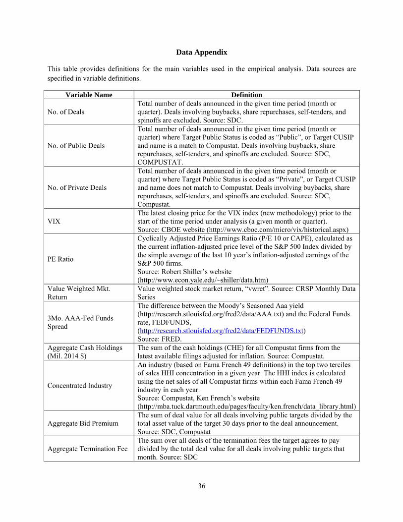
This table provides definitions for the main variables used in the empirical analysis. Data sources are specified in variable definitions.

Variable Name Definition

No. of Deals Total number of deals announced in the given time period (month or quarter). Deals involving buybacks, share repurchases, self-tenders, and spinoffs are excluded. Source: SDC.

No. of Public Deals

Total number of deals announced in the given time period (month or quarter) where Target Public Status is coded as “Public”, or Target CUSIP and name is a match to Compustat. Deals involving buybacks, share repurchases, self-tenders, and spinoffs are excluded. Source: SDC, COMPUSTAT.

No. of Private Deals

Total number of deals announced in the given time period (month or quarter) where Target Public Status is coded as “Private”, or Target CUSIP and name does not match to Compustat. Deals involving buybacks, share repurchases, self-tenders, and spinoffs are excluded. Source: SDC, Compustat.

VIX The latest closing price for the VIX index (new methodology) prior to the start of the time period under analysis (a given month or quarter). Source: CBOE website (http://www.cboe.com/micro/vix/historical.aspx)

PE Ratio

Cyclically Adjusted Price Earnings Ratio (P/E 10 or CAPE), calculated as the current inflation-adjusted price level of the S&P 500 Index divided by the simple average of the last 10 year’s inflation-adjusted earnings of the S&P 500 firms. Source: Robert Shiller’s website (http://www.econ.yale.edu/~shiller/data.htm)

Value Weighted Mkt. Return

Value weighted stock market return, “vwret”. Source: CRSP Monthly Data Series

3Mo. AAA-Fed Funds Spread

The difference between the Moody’s Seasoned Aaa yield (http://research.stlouisfed.org/fred2/data/AAA.txt) and the Federal Funds rate, FEDFUNDS, (http://research.stlouisfed.org/fred2/data/FEDFUNDS.txt) Source: FRED.

Aggregate Cash Holdings (Mil. 2014 $)

The sum of the cash holdings (CHE) for all Compustat firms from the latest available filings adjusted for inflation. Source: Compustat.

Concentrated Industry

An industry (based on Fama French 49 definitions) in the top two terciles of sales HHI concentration in a given year. The HHI index is calculated using the net sales of all Compustat firms within each Fama French 49 industry in each year. Source: Compustat, Ken French’s website (http://mba.tuck.dartmouth.edu/pages/faculty/ken.french/data_library.html)

Aggregate Bid Premium The sum of deal value for all deals involving public targets divided by the total asset value of the target 30 days prior to the deal announcement. Source: SDC, Compustat

Aggregate Termination Fee The sum over all deals of the termination fees the target agrees to pay divided by the total deal value for all deals involving public targets that month. Source: SDC

37

Table 1 – Summary Statistics

This table reports the summary statistics at a monthly frequency for the main variables used in the analysis from March 1990 to December 2013. The number of observations is 286 for all variables. The number of deals (both public and private) is obtained from the SDC Mergers and Acquisitions database. Monthly VIX is calculated as the closing price on the last day of the previous month, obtained from the CBEO website. “PE Ratio” is calculated as the Cyclically Adjusted Price Earnings Ratio (CAPE) obtained from Robert Shiller’s website. The CAPE is defined as the current inflation-adjusted price level of the S&P 500 index divided by the simple average of the last 10 year’s inflation-adjusted earnings of the S&P 500 firms. The value weighted market return is obtained from CRSP (with dividends), and the “3Mo. AAA-Fed Funds Spread” is calculated as the difference between the Moody’s seasoned Aaa yield and the federal funds rates, both obtained from the FRED website. “Aggregate cash holdings” is the sum of the latest available value for cash and short-term equivalents (CHE) for all firms in Compustat. Percent change in cash holdings is calculated at an annual level using latest available filings.

Mean Std. Dev 25th Percentile 75th Percentile

No. of Deals 692.04 168.88 572.00 807.00

No. of Public Deals 54.33 18.92 40.00 65.00

No. of Private Deals 637.70 160.27 523.00 751.00

%Δ No. of Deals 1.11% 13.33% -7.23% 8.91%

% Δ No. of Public Deals 2.52% 24.36% -14.81% 17.57%

% Δ No. of Private Deals 1.19% 13.66% -7.55% 9.00%

VIX 19.99 7.65 14.02 23.95

% Δ VIX 1.37% 18.61% -11.01% 9.61%

PE Ratio 25.31 6.85 20.54 27.27

% Δ PE Ratio 0.23% 3.59% -1.45% 2.35%

Value Weighted Mkt. Return 0.91% 4.34% -1.75% 3.77%

3Mo. AAA-Fed Funds Spread 3.09% 1.52% 1.62% 4.48%

% Δ (3Mo. AAA- Fed Funds Spread) 2.71% 31.07% -4.80% 4.94%

Aggregate Cash Holdings (Mil. 2014 $) $5,261,946 $2,605,910 $2,787,361 $7,801,380

% Δ Aggregate Cash Holdings (Mil. 2014 $) 6.36% 8.63% 2.39% 12.23%

Table 2 – Volatility and Merger Activity

This table reports the results of a monthly time-series OLS regression where the dependent variable is the percent change in the aggregate number of merger announcements for each sample indicated. The independent variables are all in percent change units, calculated with one lag with respect to the dependent variable. That is, if the dependent variable is the percent change in merger announcements from May to June 2000, the independent variable is calculated as the percent change in that respective variable from April to May 2000. Percent change in cash holdings is calculated at an annual level using latest available filings. Columns 3 and 4 of each Panel include an indicator variable for each year and calendar month (January, February, etc). Standard errors are clustered at the year-level in Column 3 of each panel whereas Newey-West standard errors are reported in Column 4 of each panel.

(1) (2) (3) (4) (1) (2) (3) (4) (1) (2) (3) (4)

Panel A: All Firms Panel B: Public Targets Panel C: Private Targets

%Δ VIX -0.03 -0.07 -0.06 -0.06 -0.11 -0.29*** -0.29** -0.29** -0.02 -0.05 -0.04 -0.04

(0.04) (0.06) (0.05) (0.05) (0.08) (0.10) (0.14) (0.12) (0.04) (0.06) (0.05) (0.05)

%Δ PE ratio 0.32 -0.05 -0.05 1.08** 0.85 0.85 0.29 -0.10 -0.10

(0.29) (0.42) (0.34) (0.53) (0.73) (0.62) (0.30) (0.43) (0.35) %Δ Value Wgt. Mkt

Return -0.00 -0.00 -0.00

-0.02*** -0.01 -0.01**

-0.00 -0.00 -0.00

(0.00) (0.00) (0.00) (0.01) (0.01) (0.01) (0.00) (0.00) (0.00) %Δ AAA-3Mo Fed

Funds Spread 0.02 0.04** 0.04**

0.01 0.01 0.01

0.02 0.04** 0.04***

(0.02) (0.02) (0.02) (0.05) (0.02) (0.02) (0.03) (0.02) (0.02)

%Δ Cash Holdings 0.01 0.00 0.00 0.05 -0.00 -0.00 0.01 0.01 0.01

(0.09) (0.03) (0.19) (0.16) (0.04) (0.43) (0.09) (0.03) (0.20)

Constant 0.01 0.01 -0.00 -0.00 0.03* 0.04** -0.19*** -0.19*** 0.01 0.01 0.02 0.02

(0.01) (0.01) (0.03) (0.03) (0.01) (0.02) (0.03) (0.06) (0.01) (0.01) (0.03) (0.03)

Observations 286 286 286 286 286 286 286 286 286 286 286 286

R-squared 0.00 0.01 0.32 0.01 0.04 0.21 0.00 0.01 0.32

Year FE No No Yes Yes No No Yes Yes No No Yes Yes

Month FE No No Yes Yes No No Yes Yes No No Yes Yes

SE Cluster None None Year Newey-West

None None Year Newey-

West None None Year

Newey-West

*** p<0.01, ** p<0.05, * p<0.1

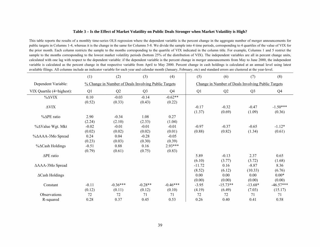
39

Table 3 – Is the Effect of Market Volatility on Public Deals Stronger when Market Volatility is High?

This table reports the results of a monthly time-series OLS regression where the dependent variable is the percent change in the aggregate number of merger announcements for public targets in Columns 1-4, whereas it is the change in the same for Columns 5-8. We divide the sample into 4 time periods, corresponding to 4 quartiles of the value of VIX for the prior month. Each column restricts the sample to the months corresponding to the quartile of VIX indicated in the column title. For example, Columns 1 and 5 restrict the sample to the months corresponding to the lowest market volatility periods (bottom 25% of the distribution of VIX). The independent variables are all in percent change units, calculated with one lag with respect to the dependent variable: if the dependent variable is the percent change in merger announcements from May to June 2000, the independent variable is calculated as the percent change in that respective variable from April to May 2000. Percent change in cash holdings is calculated at an annual level using latest available filings. All columns include an indicator variable for each year and calendar month (January, February, etc) and standard errors are clustered at the year-level.

(1) (2) (3) (4) (5) (6) (7) (8)

Dependent Variable: % Change in Number of Deals Involving Public Targets Change in Number of Deals Involving Public Targets

VIX Quartile (4=highest): Q1 Q2 Q3 Q4 Q1 Q2 Q3 Q4

%ΔVIX 0.10 -0.03 -0.14 -0.62** (0.52) (0.33) (0.43) (0.22)

ΔVIX -0.17 -0.32 -0.47 -1.50*** (1.37) (0.69) (1.09) (0.36)

%ΔPE ratio 2.90 -0.34 1.08 0.27 (2.24) (2.10) (2.33) (1.04)

%ΔValue Wgt. Mkt -0.02 -0.01 -0.01 -0.01 -0.97 -0.37 -0.65 -1.12* (0.02) (0.02) (0.02) (0.01) (0.88) (0.82) (1.34) (0.61)

%ΔAAA-3Mo Spread 0.24 0.04 -0.28 -0.05 (0.23) (0.03) (0.30) (0.39)

%ΔCash Holdings -0.51 0.88 0.16 2.93*** (0.79) (0.61) (0.75) (0.83)

ΔPE ratio 5.89 -0.13 2.37 0.65 (6.10) (3.77) (3.72) (1.68)

ΔAAA-3Mo Spread -11.72 0.16 -8.87 8.36 (8.52) (6.12) (10.33) (6.76)

ΔCash Holdings 0.00 0.00 0.00 0.00* (0.00) (0.00) (0.00) (0.00)

Constant -0.11 -0.36*** -0.28** -0.46*** -3.95 -15.73** -13.68* -46.57*** (0.12) (0.11) (0.12) (0.10) (4.19) (6.49) (7.03) (15.17)

Observations 72 72 71 71 72 72 71 71 R-squared 0.28 0.37 0.45 0.53 0.26 0.40 0.41 0.58

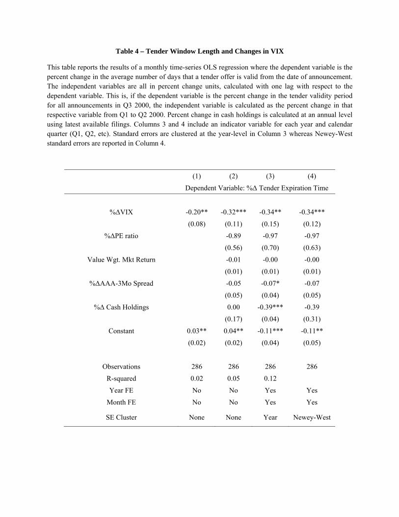
Table 4 – Tender Window Length and Changes in VIX

This table reports the results of a monthly time-series OLS regression where the dependent variable is the percent change in the average number of days that a tender offer is valid from the date of announcement. The independent variables are all in percent change units, calculated with one lag with respect to the dependent variable. This is, if the dependent variable is the percent change in the tender validity period for all announcements in Q3 2000, the independent variable is calculated as the percent change in that respective variable from Q1 to Q2 2000. Percent change in cash holdings is calculated at an annual level using latest available filings. Columns 3 and 4 include an indicator variable for each year and calendar quarter (Q1, Q2, etc). Standard errors are clustered at the year-level in Column 3 whereas Newey-West standard errors are reported in Column 4.

(1) (2) (3) (4)

Dependent Variable: %Δ Tender Expiration Time

%ΔVIX -0.20** -0.32*** -0.34** -0.34***

(0.08) (0.11) (0.15) (0.12)

%ΔPE ratio -0.89 -0.97 -0.97

(0.56) (0.70) (0.63)

Value Wgt. Mkt Return -0.01 -0.00 -0.00

(0.01) (0.01) (0.01)

%ΔAAA-3Mo Spread -0.05 -0.07* -0.07

(0.05) (0.04) (0.05)

%Δ Cash Holdings 0.00 -0.39*** -0.39

(0.17) (0.04) (0.31)

Constant 0.03** 0.04** -0.11*** -0.11**

(0.02) (0.02) (0.04) (0.05)

Observations 286 286 286 286

R-squared 0.02 0.05 0.12

Year FE No No Yes Yes

Month FE No No Yes Yes

SE Cluster None None Year Newey-West

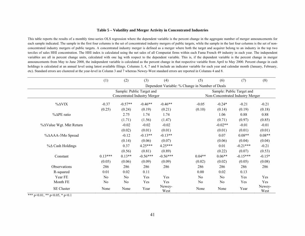
41

 

Table 5 – Volatility and Merger Activity in Concentrated Industries

This table reports the results of a monthly time-series OLS regression where the dependent variable is the percent change in the aggregate number of merger announcements for each sample indicated. The sample in the first four columns is the set of concentrated industry mergers of public targets, while the sample in the last four columns is the set of non-concentrated industry mergers of public targets. A concentrated industry merger is defined as a merger where both the target and acquirer belong to an industry in the top two terciles of sales HHI concentration. The HHI index is calculated using the net sales of all Compustat firms within each Fama French 49 industry in each year. The independent variables are all in percent change units, calculated with one lag with respect to the dependent variable. This is, if the dependent variable is the percent change in merger announcements from May to June 2000, the independent variable is calculated as the percent change in that respective variable from April to May 2000. Percent change in cash holdings is calculated at an annual level using latest available filings. Columns 3, 4, 7 and 8 include an indicator variable for each year and calendar month (January, February, etc). Standard errors are clustered at the year-level in Column 3 and 7 whereas Newey-West standard errors are reported in Columns 4 and 8.

(1) (2) (3) (4) (5) (6) (7) (8)

Dependent Variable: % Change in Number of Deals

Sample: Public Target and

Concentrated Industry Merger Sample: Public Target and

Non-Concentrated Industry Merger

%ΔVIX -0.37 -0.57** -0.46** -0.46** -0.05 -0.24* -0.21 -0.21 (0.25) (0.24) (0.19) (0.21) (0.10) (0.14) (0.19) (0.18)

%ΔPE ratio 2.75 1.74 1.74 1.06 0.88 0.88 (1.71) (1.56) (1.47) (0.71) (0.97) (0.85)

%ΔValue Wgt. Mkt Return -0.02 -0.02 -0.02 -0.02** -0.01 -0.01 (0.02) (0.01) (0.01) (0.01) (0.01) (0.01)

%ΔAAA-3Mo Spread -0.12 -0.13** -0.13** 0.07 0.08** 0.08** (0.14) (0.06) (0.07) (0.06) (0.04) (0.04)

%Δ Cash Holdings 0.37 4.25*** 4.25*** 0.01 -0.21*** -0.21 (0.56) (0.81) (0.89) (0.22) (0.07) (0.53)

Constant 0.13*** 0.13** -0.56*** -0.56*** 0.04** 0.06** -0.15*** -0.15* (0.05) (0.06) (0.09) (0.09) (0.02) (0.02) (0.05) (0.08)

Observations 286 286 286 286 286 286 286 286 R-squared 0.01 0.02 0.11 0.00 0.02 0.13 Year FE No No Yes Yes No No Yes Yes

Month FE No No Yes Yes No No Yes Yes

SE Cluster None None Year Newey-

West None None Year

Newey-West

*** p<0.01, ** p<0.05, * p<0.1

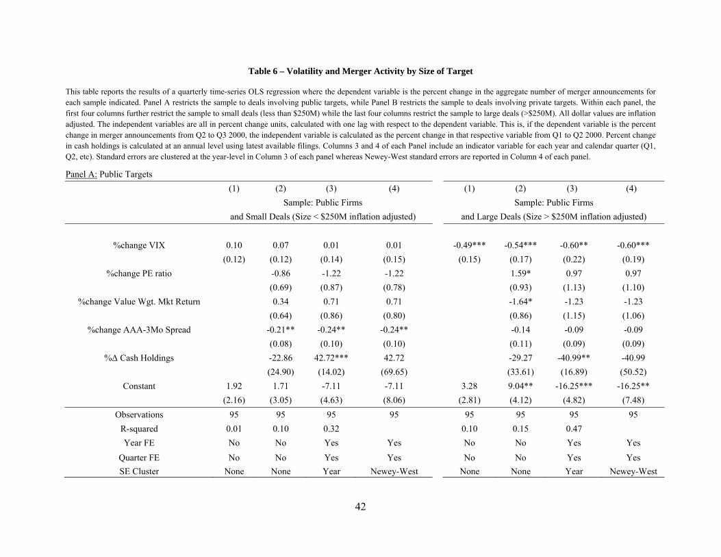
42

 

Table 6 – Volatility and Merger Activity by Size of Target

This table reports the results of a quarterly time-series OLS regression where the dependent variable is the percent change in the aggregate number of merger announcements for each sample indicated. Panel A restricts the sample to deals involving public targets, while Panel B restricts the sample to deals involving private targets. Within each panel, the first four columns further restrict the sample to small deals (less than $250M) while the last four columns restrict the sample to large deals (>$250M). All dollar values are inflation adjusted. The independent variables are all in percent change units, calculated with one lag with respect to the dependent variable. This is, if the dependent variable is the percent change in merger announcements from Q2 to Q3 2000, the independent variable is calculated as the percent change in that respective variable from Q1 to Q2 2000. Percent change in cash holdings is calculated at an annual level using latest available filings. Columns 3 and 4 of each Panel include an indicator variable for each year and calendar quarter (Q1, Q2, etc). Standard errors are clustered at the year-level in Column 3 of each panel whereas Newey-West standard errors are reported in Column 4 of each panel.

Panel A: Public Targets

(1) (2) (3) (4) (1) (2) (3) (4)

Sample: Public Firms Sample: Public Firms

and Small Deals (Size < $250M inflation adjusted) and Large Deals (Size > $250M inflation adjusted)

%change VIX 0.10 0.07 0.01 0.01 -0.49*** -0.54*** -0.60** -0.60***

(0.12) (0.12) (0.14) (0.15) (0.15) (0.17) (0.22) (0.19)

%change PE ratio -0.86 -1.22 -1.22 1.59* 0.97 0.97

(0.69) (0.87) (0.78) (0.93) (1.13) (1.10)

%change Value Wgt. Mkt Return 0.34 0.71 0.71 -1.64* -1.23 -1.23

(0.64) (0.86) (0.80) (0.86) (1.15) (1.06)

%change AAA-3Mo Spread -0.21** -0.24** -0.24** -0.14 -0.09 -0.09

(0.08) (0.10) (0.10) (0.11) (0.09) (0.09)

%Δ Cash Holdings -22.86 42.72*** 42.72 -29.27 -40.99** -40.99

(24.90) (14.02) (69.65) (33.61) (16.89) (50.52)

Constant 1.92 1.71 -7.11 -7.11 3.28 9.04** -16.25*** -16.25**

(2.16) (3.05) (4.63) (8.06) (2.81) (4.12) (4.82) (7.48)

Observations 95 95 95 95 95 95 95 95

R-squared 0.01 0.10 0.32 0.10 0.15 0.47

Year FE No No Yes Yes No No Yes Yes

Quarter FE No No Yes Yes No No Yes Yes

SE Cluster None None Year Newey-West None None Year Newey-West

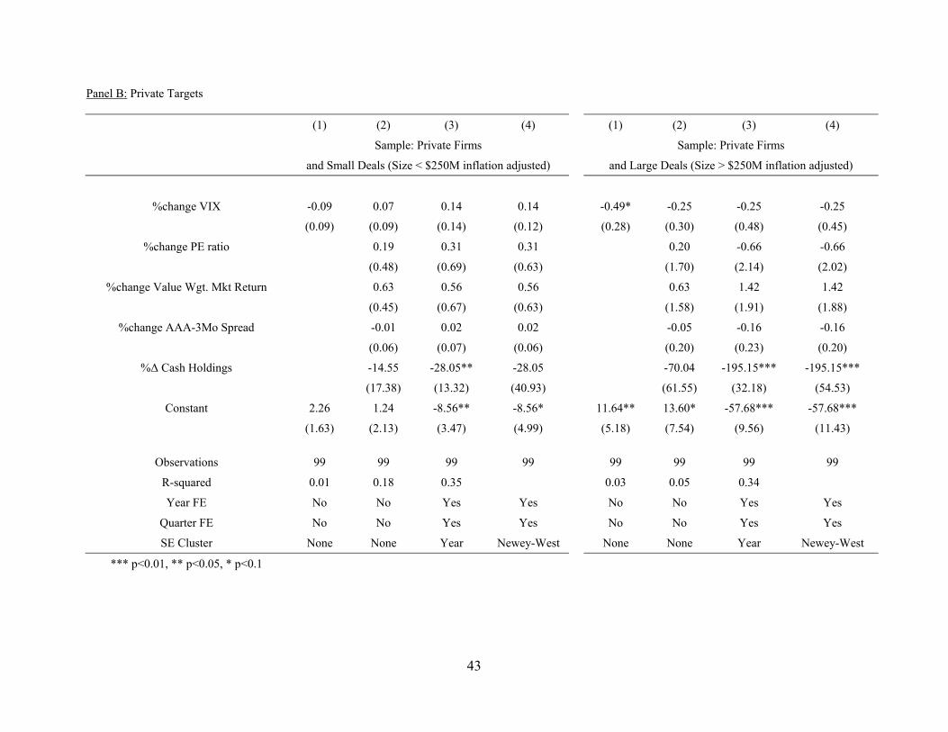
43

 

Panel B: Private Targets

(1) (2) (3) (4) (1) (2) (3) (4)

Sample: Private Firms Sample: Private Firms

and Small Deals (Size < $250M inflation adjusted) and Large Deals (Size > $250M inflation adjusted)

%change VIX -0.09 0.07 0.14 0.14 -0.49* -0.25 -0.25 -0.25

(0.09) (0.09) (0.14) (0.12) (0.28) (0.30) (0.48) (0.45)

%change PE ratio 0.19 0.31 0.31 0.20 -0.66 -0.66

(0.48) (0.69) (0.63) (1.70) (2.14) (2.02)

%change Value Wgt. Mkt Return 0.63 0.56 0.56 0.63 1.42 1.42

(0.45) (0.67) (0.63) (1.58) (1.91) (1.88)

%change AAA-3Mo Spread -0.01 0.02 0.02 -0.05 -0.16 -0.16

(0.06) (0.07) (0.06) (0.20) (0.23) (0.20)

%Δ Cash Holdings -14.55 -28.05** -28.05 -70.04 -195.15*** -195.15***

(17.38) (13.32) (40.93) (61.55) (32.18) (54.53)

Constant 2.26 1.24 -8.56** -8.56* 11.64** 13.60* -57.68*** -57.68***

(1.63) (2.13) (3.47) (4.99) (5.18) (7.54) (9.56) (11.43)

Observations 99 99 99 99 99 99 99 99

R-squared 0.01 0.18 0.35 0.03 0.05 0.34

Year FE No No Yes Yes No No Yes Yes

Quarter FE No No Yes Yes No No Yes Yes

SE Cluster None None Year Newey-West None None Year Newey-West

*** p<0.01, ** p<0.05, * p<0.1

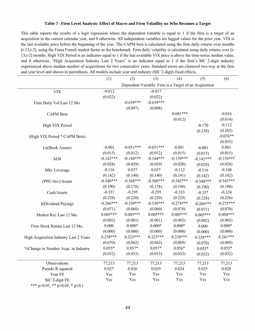
44

 

Table 7– Firm Level Analysis: Effect of Macro and Firm Volatility on Who Becomes a Target

This table reports the results of a logit regression where the dependent variable is equal to 1 if the firm is a target of an acquisition in the current calendar year, and 0 otherwise. All independent variables are lagged values for the prior year. VIX is the last available price before the beginning of the year. The CAPM beta is calculated using the firm daily returns over months [t-13,t-2], using the Fama French market factor as the benchmark. Firm daily volatility is calculated using daily returns over [t-13,t-2] months. High VIX Period is an indicator equal to 1 if the last available VIX price is above the time-series median value, and 0 otherwise. “High Acquisition Industry Last 2 Years” is an indicator equal to 1 if the firm’s SIC 2-digit industry experienced above median number of acquisitions for two consecutive years. Standard errors are clustered two-way at the firm and year level and shown in parenthesis. All models include year and industry (SIC 2-digit) fixed effects.

(1) (2) (3) (4) (5) (6)

Dependent Variable: Firm is a Target of an Acquisition

VIX -0.012 -0.017 (0.022) (0.022)

Firm Daily Vol Last 12 Mo. -0.639*** -0.639*** (0.097) (0.098)

CAPM Beta -0.041*** -0.016 (0.012) (0.014)

High VIX Period -0.170 -0.112 (0.238) (0.265)

(High VIX Period * CAPM Beta) -0.076** (0.035)

Ln(Book Assets) -0.001 -0.051*** -0.051*** 0.001 -0.001 0.001 (0.015) (0.012) (0.012) (0.015) (0.015) (0.015)

M/B -0.142*** -0.144*** -0.144*** -0.139*** -0.142*** -0.139*** (0.028) (0.029) (0.029) (0.028) (0.028) (0.028)

Mkt. Leverage -0.116 0.037 0.037 -0.112 -0.116 -0.108 (0.142) (0.140) (0.140) (0.141) (0.142) (0.142)

(PPE+Inv)/Assets -0.540*** -0.568*** -0.568*** -0.542*** -0.540*** -0.543*** (0.190) (0.178) (0.178) (0.190) (0.190) (0.190)

Cash/Assets -0.357 -0.295 -0.295 -0.333 -0.357 -0.324 (0.228) (0.220) (0.220) (0.229) (0.228) (0.226)

I(Dividend Paying) -0.266*** -0.330*** -0.330*** -0.274*** -0.266*** -0.275*** (0.071) (0.060) (0.060) (0.070) (0.071) (0.070)

Market Ret. Last 12 Mo. 0.005*** 0.005*** 0.005*** 0.005*** 0.005*** 0.004*** (0.002) (0.001) (0.001) (0.002) (0.002) (0.002)

Firm Stock Return Last 12 Mo. 0.000 0.000* 0.000* 0.000* 0.000 0.000* (0.000) (0.000) (0.000) (0.000) (0.000) (0.000)

High Acquisition Industry Last 2 Years 0.238*** 0.223*** 0.223*** 0.238*** 0.238*** 0.241*** (0.070) (0.062) (0.062) (0.069) (0.070) (0.069)

%Change in Number Acqs. in Industry 0.055* 0.057* 0.057* 0.056* 0.055* 0.055* (0.032) (0.033) (0.033) (0.032) (0.032) (0.032)

Observations 77,213 77,213 77,213 77,213 77,213 77,213 Pseudo R-squared 0.027 0.026 0.029 0.024 0.025 0.028

Year FE Yes Yes Yes Yes Yes Yes

SIC 2-digit FE Yes Yes Yes Yes Yes Yes

*** p<0.01, ** p<0.05, * p<0.1

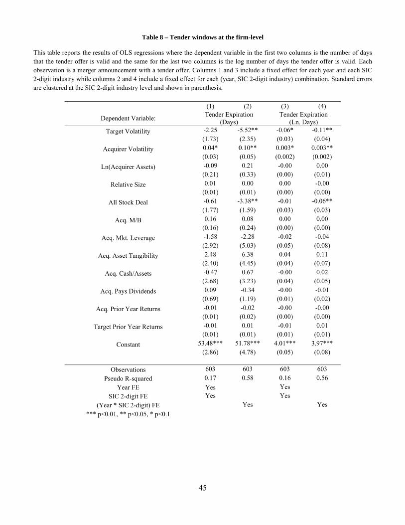
45

 

Table 8 – Tender windows at the firm-level

This table reports the results of OLS regressions where the dependent variable in the first two columns is the number of days that the tender offer is valid and the same for the last two columns is the log number of days the tender offer is valid. Each observation is a merger announcement with a tender offer. Columns 1 and 3 include a fixed effect for each year and each SIC 2-digit industry while columns 2 and 4 include a fixed effect for each (year, SIC 2-digit industry) combination. Standard errors are clustered at the SIC 2-digit industry level and shown in parenthesis.

(1) (2) (3) (4)

Dependent Variable: Tender Expiration

(Days) Tender Expiration

(Ln. Days) Target Volatility -2.25 -5.52** -0.06* -0.11**

(1.73) (2.35) (0.03) (0.04)

Acquirer Volatility 0.04* 0.10** 0.003* 0.003** (0.03) (0.05) (0.002) (0.002)

Ln(Acquirer Assets) -0.09 0.21 -0.00 0.00 (0.21) (0.33) (0.00) (0.01)

Relative Size 0.01 0.00 0.00 -0.00 (0.01) (0.01) (0.00) (0.00)

All Stock Deal -0.61 -3.38** -0.01 -0.06** (1.77) (1.59) (0.03) (0.03)

Acq. M/B 0.16 0.08 0.00 0.00 (0.16) (0.24) (0.00) (0.00)

Acq. Mkt. Leverage -1.58 -2.28 -0.02 -0.04 (2.92) (5.03) (0.05) (0.08)

Acq. Asset Tangibility 2.48 6.38 0.04 0.11 (2.40) (4.45) (0.04) (0.07)

Acq. Cash/Assets -0.47 0.67 -0.00 0.02 (2.68) (3.23) (0.04) (0.05)

Acq. Pays Dividends 0.09 -0.34 -0.00 -0.01 (0.69) (1.19) (0.01) (0.02)

Acq. Prior Year Returns -0.01 -0.02 -0.00 -0.00 (0.01) (0.02) (0.00) (0.00)

Target Prior Year Returns -0.01 0.01 -0.01 0.01

(0.01) (0.01) (0.01) (0.01)

Constant 53.48*** 51.78*** 4.01*** 3.97***

(2.86) (4.78) (0.05) (0.08)

Observations 603 603 603 603

Pseudo R-squared 0.17 0.58 0.16 0.56

Year FE Yes Yes

SIC 2-digit FE Yes Yes

(Year * SIC 2-digit) FE Yes Yes

*** p<0.01, ** p<0.05, * p<0.1

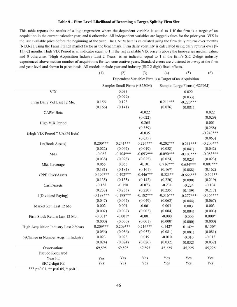
46

 

Table 9 – Firm Level Likelihood of Becoming a Target, Split by Firm Size

This table reports the results of a logit regression where the dependent variable is equal to 1 if the firm is a target of an acquisition in the current calendar year, and 0 otherwise. All independent variables are lagged values for the prior year. VIX is the last available price before the beginning of the year. The CAPM beta is calculated using the firm daily returns over months [t-13,t-2], using the Fama French market factor as the benchmark. Firm daily volatility is calculated using daily returns over [t-13,t-2] months. High VIX Period is an indicator equal to 1 if the last available VIX price is above the time-series median value, and 0 otherwise. “High Acquisition Industry Last 2 Years” is an indicator equal to 1 if the firm’s SIC 2-digit industry experienced above median number of acquisitions for two consecutive years. Standard errors are clustered two-way at the firm and year level and shown in parenthesis. All models include year and industry (SIC 2-digit) fixed effects.

(1) (2) (3) (4) (5) (6)

Dependent Variable: Firm is a Target of an Acquisition

Sample: Small Firms (<$250M) Sample: Large Firms (>$250M)

VIX 0.033 0.022 (0.099) (0.033)

Firm Daily Vol Last 12 Mo. 0.156 0.123 -0.211*** -0.220*** (0.166) (0.141) (0.076) (0.081)

CAPM Beta -0.022 0.022 (0.022) (0.029)

High VIX Period -0.265 0.001 (0.359) (0.258)

(High VIX Period * CAPM Beta) -0.035 -0.248*** (0.035) (0.063)

Ln(Book Assets) 0.200*** 0.241*** 0.226*** -0.202*** -0.211*** -0.200*** (0.022) (0.047) (0.019) (0.038) (0.041) (0.042)

M/B -0.062 -0.104*** -0.093*** -0.090*** -0.103*** -0.083*** (0.038) (0.023) (0.025) (0.024) (0.023) (0.023)

Mkt. Leverage 0.055 0.055 -0.101 0.716*** 0.654*** 0.801*** (0.181) (0.181) (0.161) (0.167) (0.088) (0.162)

(PPE+Inv)/Assets -0.490*** -0.492*** -0.446*** -0.523** -0.666*** -0.504** (0.135) (0.135) (0.142) (0.220) (0.090) (0.219)

Cash/Assets -0.158 -0.158 -0.073 -0.231 -0.224 -0.104 (0.233) (0.233) (0.220) (0.235) (0.139) (0.217)

I(Dividend Paying) -0.198*** -0.198*** -0.182*** -0.316*** -0.277*** -0.364*** (0.047) (0.047) (0.049) (0.063) (0.044) (0.067)

Market Ret. Last 12 Mo. 0.002 0.001 -0.001 0.003 0.003 0.003 (0.002) (0.002) (0.002) (0.004) (0.004) (0.003)

Firm Stock Return Last 12 Mo. -0.001* -0.001* -0.001 -0.000 -0.000 0.000* (0.000) (0.000) (0.001) (0.000) (0.000) (0.000)

High Acquisition Industry Last 2 Years 0.209*** 0.209*** 0.216*** 0.142* 0.142* 0.150* (0.056) (0.056) (0.057) (0.081) (0.081) (0.081)

%Change in Number Acqs. in Industry 0.023 0.023 0.019 -0.010 -0.010 -0.013 (0.024) (0.024) (0.026) (0.032) (0.032) (0.032)

Observations 69,595 69,595 69,595 45,225 45,225 45,225 Pseudo R-squared

Year FE Yes Yes Yes Yes Yes Yes

SIC 2-digit FE Yes Yes Yes Yes Yes Yes

*** p<0.01, ** p<0.05, * p<0.1

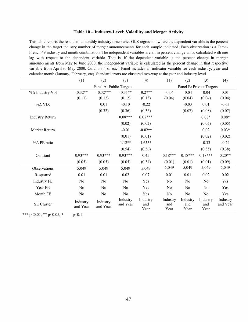
47

 

Table 10 – Industry-Level: Volatility and Merger Activity

This table reports the results of a monthly industry time-series OLS regression where the dependent variable is the percent change in the target industry number of merger announcements for each sample indicated. Each observation is a Fama-French 49 industry and month combination. The independent variables are all in percent change units, calculated with one lag with respect to the dependent variable. That is, if the dependent variable is the percent change in merger announcements from May to June 2000, the independent variable is calculated as the percent change in that respective variable from April to May 2000. Columns 4 of each Panel includes an indicator variable for each industry, year and calendar month (January, February, etc). Standard errors are clustered two-way at the year and industry level.

(1) (2) (3) (4) (1) (2) (3) (4)

Panel A: Public Targets Panel B: Private Targets

%Δ Industry Vol -0.32** -0.32*** -0.31** -0.27** -0.04 -0.04 -0.04 0.01 (0.11) (0.12) (0.12) (0.13) (0.04) (0.04) (0.04) (0.04)

%Δ VIX 0.01 -0.10 -0.22 -0.03 0.01 -0.03

(0.32) (0.36) (0.36) (0.07) (0.08) (0.07)

Industry Return 0.08*** 0.07*** 0.08* 0.08*

(0.02) (0.02) (0.05) (0.05)

Market Return -0.01 -0.02** 0.02 0.03*

(0.01) (0.01) (0.02) (0.02)

%Δ PE ratio 1.12** 1.65** -0.33 -0.24

(0.54) (0.56) (0.35) (0.38)

Constant 0.93*** 0.93*** 0.93*** 0.45 0.18*** 0.18*** 0.18*** 0.20**

(0.05) (0.05) (0.05) (0.34) (0.01) (0.01) (0.01) (0.09)

Observations 5,049 5,049 5,049 5,049 5,049 5,049 5,049 5,049

R-squared 0.01 0.01 0.02 0.07 0.01 0.01 0.02 0.02

Industry FE No No No Yes No No No Yes

Year FE No No No Yes No No No Yes

Month FE No No No Yes No No No Yes

SE Cluster Industry and Year

Industry and Year

Industry and Year

Industry and

Year

Industry and Year

Industry and Year

Industry and Year

Industry and Year

*** p<0.01, ** p<0.05, * p<0.1

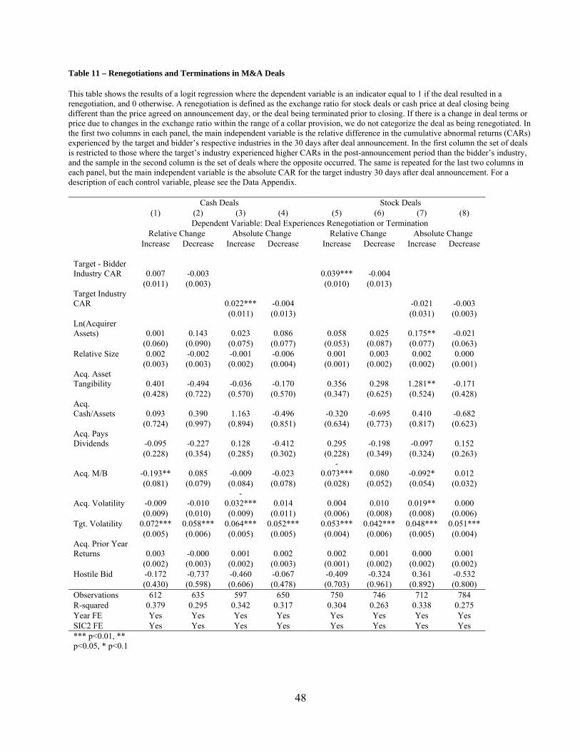
48

 

Table 11 – Renegotiations and Terminations in M&A Deals

This table shows the results of a logit regression where the dependent variable is an indicator equal to 1 if the deal resulted in a renegotiation, and 0 otherwise. A renegotiation is defined as the exchange ratio for stock deals or cash price at deal closing being different than the price agreed on announcement day, or the deal being terminated prior to closing. If there is a change in deal terms or price due to changes in the exchange ratio within the range of a collar provision, we do not categorize the deal as being renegotiated. In the first two columns in each panel, the main independent variable is the relative difference in the cumulative abnormal returns (CARs) experienced by the target and bidder’s respective industries in the 30 days after deal announcement. In the first column the set of deals is restricted to those where the target’s industry experienced higher CARs in the post-announcement period than the bidder’s industry, and the sample in the second column is the set of deals where the opposite occurred. The same is repeated for the last two columns in each panel, but the main independent variable is the absolute CAR for the target industry 30 days after deal announcement. For a description of each control variable, please see the Data Appendix.

Cash Deals Stock Deals (1) (2) (3) (4) (5) (6) (7) (8) Dependent Variable: Deal Experiences Renegotiation or Termination

Relative Change Absolute Change Relative Change Absolute Change Increase Decrease Increase Decrease Increase Decrease Increase Decrease

Target - Bidder Industry CAR 0.007 -0.003 0.039*** -0.004

(0.011) (0.003) (0.010) (0.013) Target Industry CAR 0.022*** -0.004 -0.021 -0.003

(0.011) (0.013) (0.031) (0.003) Ln(Acquirer Assets) 0.001 0.143 0.023 0.086 0.058 0.025 0.175** -0.021

(0.060) (0.090) (0.075) (0.077) (0.053) (0.087) (0.077) (0.063) Relative Size 0.002 -0.002 -0.001 -0.006 0.001 0.003 0.002 0.000

(0.003) (0.003) (0.002) (0.004) (0.001) (0.002) (0.002) (0.001) Acq. Asset Tangibility 0.401 -0.494 -0.036 -0.170 0.356 0.298 1.281** -0.171

(0.428) (0.722) (0.570) (0.570) (0.347) (0.625) (0.524) (0.428) Acq. Cash/Assets 0.093 0.390 1.163 -0.496 -0.320 -0.695 0.410 -0.682

(0.724) (0.997) (0.894) (0.851) (0.634) (0.773) (0.817) (0.623) Acq. Pays Dividends -0.095 -0.227 0.128 -0.412 0.295 -0.198 -0.097 0.152

(0.228) (0.354) (0.285) (0.302) (0.228) (0.349) (0.324) (0.263)

Acq. M/B -0.193** 0.085 -0.009 -0.023 -

0.073*** 0.080 -0.092* 0.012 (0.081) (0.079) (0.084) (0.078) (0.028) (0.052) (0.054) (0.032)

Acq. Volatility -0.009 -0.010 -

0.032*** 0.014 0.004 0.010 0.019** 0.000 (0.009) (0.010) (0.009) (0.011) (0.006) (0.008) (0.008) (0.006)

Tgt. Volatility 0.072*** 0.058*** 0.064*** 0.052*** 0.053*** 0.042*** 0.048*** 0.051*** (0.005) (0.006) (0.005) (0.005) (0.004) (0.006) (0.005) (0.004)

Acq. Prior Year Returns 0.003 -0.000 0.001 0.002 0.002 0.001 0.000 0.001

(0.002) (0.003) (0.002) (0.003) (0.001) (0.002) (0.002) (0.002) Hostile Bid -0.172 -0.737 -0.460 -0.067 -0.409 -0.324 0.361 -0.532

(0.430) (0.598) (0.606) (0.478) (0.703) (0.961) (0.892) (0.800) Observations 612 635 597 650 750 746 712 784 R-squared 0.379 0.295 0.342 0.317 0.304 0.263 0.338 0.275 Year FE Yes Yes Yes Yes Yes Yes Yes Yes SIC2 FE Yes Yes Yes Yes Yes Yes Yes Yes *** p<0.01, ** p<0.05, * p<0.1

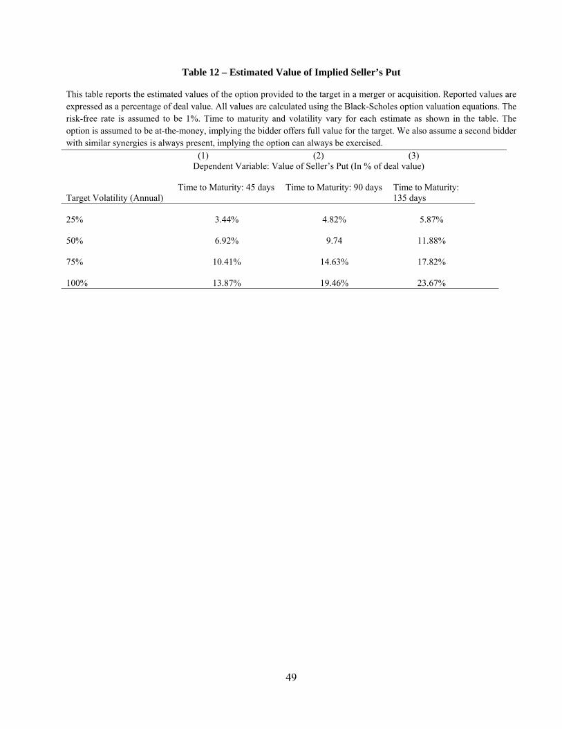
49

 

Table 12 – Estimated Value of Implied Seller’s Put

This table reports the estimated values of the option provided to the target in a merger or acquisition. Reported values are expressed as a percentage of deal value. All values are calculated using the Black-Scholes option valuation equations. The risk-free rate is assumed to be 1%. Time to maturity and volatility vary for each estimate as shown in the table. The option is assumed to be at-the-money, implying the bidder offers full value for the target. We also assume a second bidder with similar synergies is always present, implying the option can always be exercised.

(1) (2) (3) Dependent Variable: Value of Seller’s Put (In % of deal value)

Target Volatility (Annual)

Time to Maturity: 45 days Time to Maturity: 90 days Time to Maturity: 135 days

25% 3.44% 4.82% 5.87% 50% 6.92% 9.74 11.88% 75% 10.41% 14.63% 17.82% 100% 13.87% 19.46% 23.67%

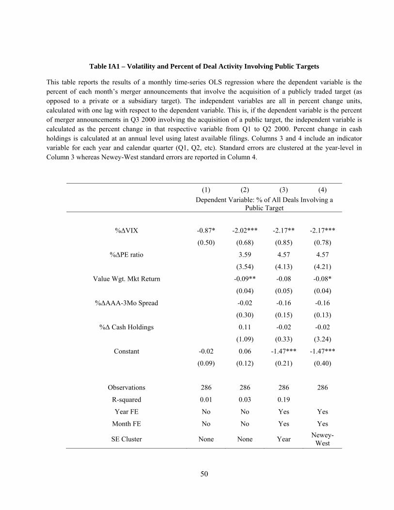
50

 

Table IA1 – Volatility and Percent of Deal Activity Involving Public Targets

This table reports the results of a monthly time-series OLS regression where the dependent variable is the percent of each month’s merger announcements that involve the acquisition of a publicly traded target (as opposed to a private or a subsidiary target). The independent variables are all in percent change units, calculated with one lag with respect to the dependent variable. This is, if the dependent variable is the percent of merger announcements in Q3 2000 involving the acquisition of a public target, the independent variable is calculated as the percent change in that respective variable from Q1 to Q2 2000. Percent change in cash holdings is calculated at an annual level using latest available filings. Columns 3 and 4 include an indicator variable for each year and calendar quarter (Q1, Q2, etc). Standard errors are clustered at the year-level in Column 3 whereas Newey-West standard errors are reported in Column 4.

(1) (2) (3) (4)

Dependent Variable: % of All Deals Involving a

Public Target

%ΔVIX -0.87* -2.02*** -2.17** -2.17***

(0.50) (0.68) (0.85) (0.78)

%ΔPE ratio 3.59 4.57 4.57

(3.54) (4.13) (4.21)

Value Wgt. Mkt Return -0.09** -0.08 -0.08*

(0.04) (0.05) (0.04)

%ΔAAA-3Mo Spread -0.02 -0.16 -0.16

(0.30) (0.15) (0.13)

%Δ Cash Holdings 0.11 -0.02 -0.02

(1.09) (0.33) (3.24)

Constant -0.02 0.06 -1.47*** -1.47***

(0.09) (0.12) (0.21) (0.40)

Observations 286 286 286 286

R-squared 0.01 0.03 0.19

Year FE No No Yes Yes

Month FE No No Yes Yes

SE Cluster None None Year Newey-

West

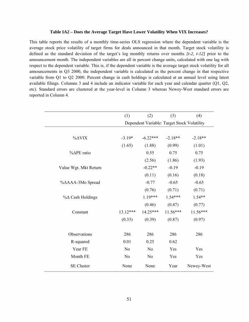
51

 

Table IA2 – Does the Average Target Have Lower Volatility When VIX Increases?

This table reports the results of a monthly time-series OLS regression where the dependent variable is the average stock price volatility of target firms for deals announced in that month. Target stock volatility is defined as the standard deviation of the target’s log monthly returns over months [t-2, t-12] prior to the announcement month. The independent variables are all in percent change units, calculated with one lag with respect to the dependent variable. This is, if the dependent variable is the average target stock volatility for all announcements in Q3 2000, the independent variable is calculated as the percent change in that respective variable from Q1 to Q2 2000. Percent change in cash holdings is calculated at an annual level using latest available filings. Columns 3 and 4 include an indicator variable for each year and calendar quarter (Q1, Q2, etc). Standard errors are clustered at the year-level in Column 3 whereas Newey-West standard errors are reported in Column 4.

(1) (2) (3) (4)

Dependent Variable: Target Stock Volatility

%ΔVIX -3.19* -6.22*** -2.18** -2.18**

(1.65) (1.88) (0.99) (1.01)

%ΔPE ratio 0.55 0.75 0.75

(2.56) (1.86) (1.93)

Value Wgt. Mkt Return -0.22** -0.19 -0.19

(0.11) (0.16) (0.18)

%ΔAAA-3Mo Spread -0.77 -0.65 -0.65

(0.76) (0.71) (0.71)

%Δ Cash Holdings 1.19*** 1.54*** 1.54**

(0.46) (0.47) (0.77)

Constant 13.12*** 14.25*** 11.56*** 11.56***

(0.33) (0.39) (0.87) (0.97)

Observations 286 286 286 286

R-squared 0.01 0.25 0.62

Year FE No No Yes Yes

Month FE No No Yes Yes

SE Cluster None None Year Newey-West

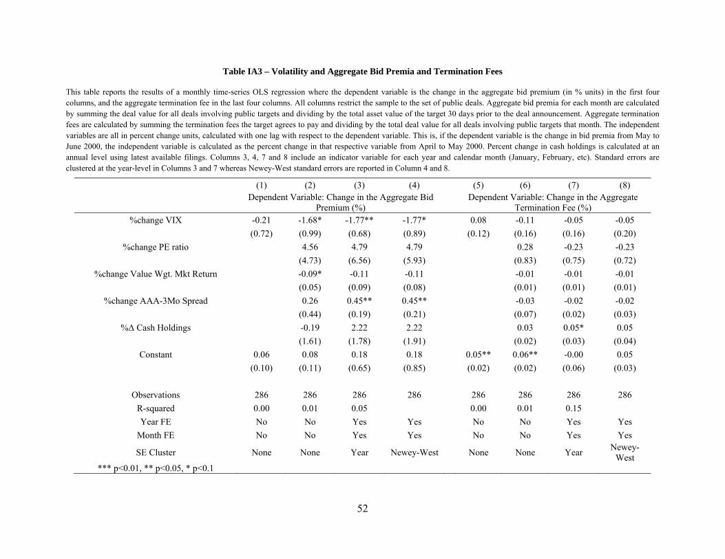
52

 

Table IA3 – Volatility and Aggregate Bid Premia and Termination Fees

This table reports the results of a monthly time-series OLS regression where the dependent variable is the change in the aggregate bid premium (in % units) in the first four columns, and the aggregate termination fee in the last four columns. All columns restrict the sample to the set of public deals. Aggregate bid premia for each month are calculated by summing the deal value for all deals involving public targets and dividing by the total asset value of the target 30 days prior to the deal announcement. Aggregate termination fees are calculated by summing the termination fees the target agrees to pay and dividing by the total deal value for all deals involving public targets that month. The independent variables are all in percent change units, calculated with one lag with respect to the dependent variable. This is, if the dependent variable is the change in bid premia from May to June 2000, the independent variable is calculated as the percent change in that respective variable from April to May 2000. Percent change in cash holdings is calculated at an annual level using latest available filings. Columns 3, 4, 7 and 8 include an indicator variable for each year and calendar month (January, February, etc). Standard errors are clustered at the year-level in Columns 3 and 7 whereas Newey-West standard errors are reported in Column 4 and 8.

(1) (2) (3) (4) (5) (6) (7) (8)

Dependent Variable: Change in the Aggregate Bid

Premium (%)

Dependent Variable: Change in the Aggregate Termination Fee (%)

%change VIX -0.21 -1.68* -1.77** -1.77* 0.08 -0.11 -0.05 -0.05

(0.72) (0.99) (0.68) (0.89) (0.12) (0.16) (0.16) (0.20)

%change PE ratio 4.56 4.79 4.79 0.28 -0.23 -0.23

(4.73) (6.56) (5.93) (0.83) (0.75) (0.72)

%change Value Wgt. Mkt Return -0.09* -0.11 -0.11 -0.01 -0.01 -0.01

(0.05) (0.09) (0.08) (0.01) (0.01) (0.01)

%change AAA-3Mo Spread 0.26 0.45** 0.45** -0.03 -0.02 -0.02

(0.44) (0.19) (0.21) (0.07) (0.02) (0.03)

%Δ Cash Holdings -0.19 2.22 2.22 0.03 0.05* 0.05

(1.61) (1.78) (1.91) (0.02) (0.03) (0.04)

Constant 0.06 0.08 0.18 0.18 0.05** 0.06** -0.00 0.05

(0.10) (0.11) (0.65) (0.85) (0.02) (0.02) (0.06) (0.03)

Observations 286 286 286 286 286 286 286 286

R-squared 0.00 0.01 0.05 0.00 0.01 0.15

Year FE No No Yes Yes No No Yes Yes

Month FE No No Yes Yes No No Yes Yes

SE Cluster None None Year Newey-West None None Year Newey-

West *** p<0.01, ** p<0.05, * p<0.1

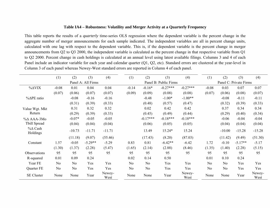
Table IA4 – Robustness: Volatility and Merger Activity at a Quarterly Frequency

This table reports the results of a quarterly time-series OLS regression where the dependent variable is the percent change in the aggregate number of merger announcements for each sample indicated. The independent variables are all in percent change units, calculated with one lag with respect to the dependent variable. This is, if the dependent variable is the percent change in merger announcements from Q2 to Q3 2000, the independent variable is calculated as the percent change in that respective variable from Q1 to Q2 2000. Percent change in cash holdings is calculated at an annual level using latest available filings. Columns 3 and 4 of each Panel include an indicator variable for each year and calendar quarter (Q1, Q2, etc). Standard errors are clustered at the year-level in Column 3 of each panel whereas Newey-West standard errors are reported in Column 4 of each panel.

(1) (2) (3) (4) (1) (2) (3) (4) (1) (2) (3) (4) Panel A: All Firms Panel B: Public Firms Panel C: Private Firms

%ΔVIX -0.08 0.01 0.04 0.04 -0.14 -0.16* -0.27*** -0.27*** -0.08 0.03 0.07 0.07 (0.07) (0.06) (0.07) (0.07) (0.09) (0.09) (0.08) (0.08) (0.07) (0.06) (0.08) (0.07)

%ΔPE ratio -0.08 -0.16 -0.16 -0.48 -1.00* -1.00** -0.08 -0.11 -0.11 (0.31) (0.39) (0.33) (0.48) (0.57) (0.47) (0.32) (0.39) (0.33)

Value Wgt. Mkt Return

0.31 0.32 0.32 0.02 0.42 0.42 0.37 0.34 0.34 (0.29) (0.39) (0.33) (0.45) (0.49) (0.44) (0.29) (0.40) (0.34)

%Δ AAA-3Mo Tbill Spread

-0.07* -0.05 -0.05 -0.17*** -0.18*** -0.18*** -0.06 -0.04 -0.04 (0.04) (0.04) (0.04) (0.06) (0.05) (0.05) (0.04) (0.04) (0.04)

%Δ Cash Holdings

-10.73 -11.71 -11.71 13.49 15.24* 15.24 -10.00 -15.28 -15.28

(11.18) (9.07) (55.46) (17.43) (8.20) (87.03) (11.42) (9.49) (51.30) Constant 1.57 -0.05 -5.29** -5.29 0.83 0.81 -6.42** -6.42 1.72 -0.10 -5.17** -5.17

(1.30) (1.37) (2.28) (5.47) (1.65) (2.14) (2.88) (8.46) (1.35) (1.40) (2.28) (5.15) Observations 95 95 95 95 95 95 95 95 95 95 95 95

R-squared 0.01 0.09 0.24 0.02 0.14 0.50 0.01 0.10 0.24 Year FE No No Yes Yes No No Yes Yes No No Yes Yes

Quarter FE No No Yes Yes No No Yes Yes No No Yes Yes

SE Cluster None None Year Newey-

West None None Year

Newey-West

None None Year Newey-

West

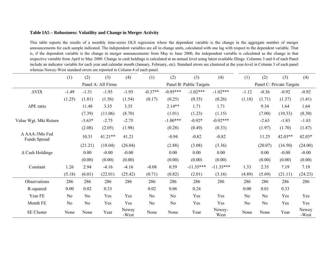
Table IA5 – Robustness: Volatility and Change in Merger Activity

This table reports the results of a monthly time-series OLS regression where the dependent variable is the change in the aggregate number of merger announcements for each sample indicated. The independent variables are all in change units, calculated with one lag with respect to the dependent variable. That is, if the dependent variable is the change in merger announcements from May to June 2000, the independent variable is calculated as the change in that respective variable from April to May 2000. Change in cash holdings is calculated at an annual level using latest available filings. Columns 3 and 4 of each Panel include an indicator variable for each year and calendar month (January, February, etc). Standard errors are clustered at the year-level in Column 3 of each panel whereas Newey-West standard errors are reported in Column 4 of each panel.

(1) (2) (3) (4) (1) (2) (3) (4) (1) (2) (3) (4)

Panel A: All Firms Panel B: Public Targets Panel C: Private Targets

ΔVIX -1.49 -1.31 -1.93 -1.93 -0.37** -0.95*** -1.02*** -1.02*** -1.12 -0.36 -0.92 -0.92

(1.25) (1.81) (1.56) (1.54) (0.17) (0.25) (0.35) (0.26) (1.18) (1.71) (1.37) (1.41)

ΔPE ratio 11.48 3.35 3.35 2.14** 1.71 1.71 9.34 1.64 1.64

(7.39) (11.06) (8.70) (1.01) (1.23) (1.15) (7.00) (10.33) (8.30)

Value Wgt. Mkt Return -3.63* -2.75 -2.75 -1.00*** -0.92* -0.92*** -2.63 -1.83 -1.83

(2.08) (2.05) (1.98) (0.28) (0.49) (0.33) (1.97) (1.70) (1.87) Δ AAA-3Mo Fed

Funds Spread 10.31 41.21** 41.21

-0.94 -0.82 -0.82

11.25 42.03** 42.03*

(21.21) (18.04) (26.04) (2.88) (3.08) (3.36) (20.07) (16.50) (24.00)

Δ Cash Holdings 0.00 -0.00 -0.00 0.00 0.00 0.00 0.00 -0.00 -0.00

(0.00) (0.00) (0.00) (0.00) (0.00) (0.00) (0.00) (0.00) (0.00)

Constant 1.26 2.94 -4.16 -4.16 -0.08 0.59 -11.35*** -11.35*** 1.33 2.35 7.19 7.19

(5.18) (6.01) (22.01) (25.42) (0.71) (0.82) (2.01) (3.16) (4.89) (5.69) (21.11) (24.23)

Observations 286 286 286 286 286 286 286 286 286 286 286 286

R-squared 0.00 0.02 0.33 0.02 0.06 0.24 0.00 0.01 0.33

Year FE No No Yes Yes No No Yes Yes No No Yes Yes

Month FE No No Yes Yes No No Yes Yes No No Yes Yes

SE Cluster None None Year Newey-West

None None Year Newey-

West None None Year

Newey-West

Internet Appendix

Here, we detail the additional tests and robustness checks summarized in Section 7 of the main

text.

A. The Effect of Volatility on the Mix of Private and Public Targets

We have hypothesized that increases in volatility increase the value of the put provided to

targets by bidders, and that this concern should affect public targets more than private targets.

This difference suggests an aggregate effect—the mix of public and private targets should tilt

away from public targets when volatility increases. In Table IA1, we estimate a specification

designed to explain the fraction of deal activity involving public targets. Again, the explanatory

variable of interest is the percent change in VIX. Consistent with a stronger effect of volatility on

the attractiveness of public targets, the fraction of deal activity involving public targets decreases

following an increase in VIX. In particular, a 1 percent increase in VIX is associated with a 2.17

percent decline in the share of announced deals consisting of a public target.

B. The Effect of Volatility on Target Selection

Just as the effect of an increase in volatility will have a larger impact on the value of the put

written to public shareholders, within public firms the effect should be larger for targets that

were more volatile to begin with, as these firms are more susceptible to overall increases in

uncertainty. In Table IA2, we explain the average volatility of targets in a given month as a

function of several variables, including our variable of interest, the change in VIX. We show that

following an increase in VIX, the average volatility (computed over months [t-13, t-2] prior to

announcement) of firms announced as targets significantly declines. A one percent increase in

VIX is associated with a 2.18 percent decline in the average target’s prior monthly volatility.

56

 

Thus, consistent with the findings on systematic risk exposure, the increase in aggregate price

volatility affects deals involving the most volatile firms, such that the distribution of observed

deals shifts toward more stable firms, as those deals should be less affected by the increased

uncertainty.

C. Interim Risk and Deal Terms

When market expectations of volatility increase, our mechanism predicts that the

marginal deal will become negative NPV regardless of the (a)symmetry of the risk, and so the

bidder will decide to delay the offer. However, the synergy in the average deal should still be

high enough to overcome the increased costs caused by the high volatility. However, if the

interim risk is at least somewhat asymmetrically borne, we expect other deal terms to adjust as

the amount of interim risk changes (Bhagwat and Dam, 2014). In this section, we assess whether

bid premia and termination fees adjust in a way that is consistent with some asymmetry in the

interim risk. In particular, we predict that increases in market-wide volatility will be associated

with decreases in average bid premia.

Similarly, acquirers may also demand a higher termination fee during times of high VIX.

However, the prevailing court precedents set 3-4% of deal value as an approximate upper bound

on the termination fee that a target must pay (Gilson and Schwartz, 2005). To the extent that this

is a binding constraint, we expect a smaller effect of VIX on termination fees.

Table IA3 presents the results of OLS time-series regressions where the dependent

variable is either the aggregate bid premium (Columns 1 through 4) or weighted average

termination fee (Columns 5 through 8) in all announced mergers in our sample in a given month

(both measures are weighted averages by deal value). We calculate bid premium as the total deal

57

 

value of all deals for public targets reported in SDC divided by the market value of assets of the

target 30 days prior to the announcement. Termination fee is calculated as the amount the target

agrees to pay if the deal is not consummated, as a percentage of the total deal value.

For univariate tests of bid premia, the coefficient on the percent change in VIX is

negative, albeit not statistically significant. However, after including our other controls, the

effect of volatility on aggregate bid premia is negative and statistically significant. The economic

magnitude is substantial as well: a 10% increase in VIX reduces bid premia in aggregate by

17.4%. For termination fees, the sign on the percent change is VIX is negative but is not

statistically significant in any of the specifications. As explained earlier, one reason for the

insignificant association between VIX and termination fees may be that the upper-bound on such

fees placed by prevailing court rulings is a binding constraint for firms.

The fact that market-wide volatility expectations affect bid premia is consistent with the

“seller’s put” having a real impact on not only deal activity, but also on deal terms for those

deals that are initiated (Bhagwat and Dam, 2014). In particular, the finding of lower offered

premiums during times of increased volatility is consistent with firms incorporating the value of

the option into deal terms. On the other hand, these findings are not consistent with a symmetric

view of the interim risk where both parties have the ability to back away from the deal ex post.

It may be surprising that the deal terms cannot fully adjust to leave the deal flow unaffected.

However, as we discuss, constraints such as precedent-driven restrictions on termination fees, a

floor of zero on feasible premiums (and likely higher given the need to satisfy a fairness

opinion), and the difficulty of assigning a value to a collar, along with enforcement uncertainty,

all limit the ability of the other deal terms to simply adjust to negate the effect of uncertainty.

58

 

D. Main Results at a Quarterly Frequency

Since our main analysis is at a monthly frequency while our size-matched results in

Section 4.D are at a quarterly frequency (due to lack of observations in some months), we re-

estimate our main analysis at a quarterly frequency as well to show our other results are robust at

that frequency.

The results, presented in Table IA4, show that we obtain a similar negative and

statistically significant relationship between percent change in VIX and quarterly percent change

in merger announcements, but again only for public targets. There is no statistically significant

effect of volatility on merger activity for the set of private target deals or for merger

announcements overall. Moreover, the estimated elasticity of quarterly merger activity with

respect to VIX is -0.27, virtually identical to the estimated elasticity at the monthly frequency (-

0.29). Note that in the full specification, we include all our controls and indicators for each year

and calendar quarter, and cluster standard errors at the year-level. We also conduct a Newey-

West standard error correction in the last column and obtain statistically significant results.

Thus, our main finding of a negative relationship between forward looking volatility and

aggregate merger activity is robust to using a monthly or quarterly frequency.

E. Change in Level of Deals Instead of Percent Change

Thus far we have analyzed deal activity as a percent change in the number of deals in

each month or quarter. An equally informative method to measure deal flow is to analyze the raw

change in the number of deals, as opposed to the percent change. While our mechanism is

59

 

agnostic to which measurement is more appropriate, we confirm in this subsection that our

results are robust to either method.

Table IA5 reports the results of an OLS monthly time-series regression where the

dependent variable is the change in the number of merger announcements for each month. The

sample consists of all merger announcements in Panel A, only public targets in Panel B, and only

private targets in Panel C. All independent variables are expressed as a change in their respective

variables, except for the value weighted market return (which is a percentage).

The results are very similar to our prior results in Table 2, where we employed the

percentage change in each variable. A change in VIX has no association with a change in

aggregate deal activity. It is only when the target is a publicly traded firm do we see that a

change in VIX is associated with a decline in the monthly number of merger announcements.

Confirming our earlier findings, we find no association between a change in VIX and deal

activity for privately held targets.

Our results are thus robust to measuring deal flow as either percentage changes or the

change in levels.