The pros and cons of the computational design of the

olfactory systemRamon Huerta

BioCircuits Institute,University California, San Diego

Deconstructing the Sense of Smell—June/19/2015

Looking at the problem as an engineer

• What’s the computational problem?• The role of fan-in/fan-out structure in the

brain.• The equivalence with machine learning

algorithms.• Gain control: What for and how?

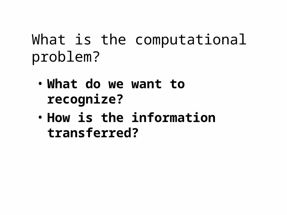
• What do we want to recognize?• How is the information transferred?

What is the computational problem?

100 200 300 400 500 600 700 800 900 1000 1100

2000

4000

6000

Se

nso

r

Re

spo

nse

()

100 200 300 400 500-1

0

1

em

a max

=

0.00

1

Features considered in the rising portionof the sensor response

100 200 300 400 500-2

0

2

em

a max

=

0.01

600 700 800 900 1000 1100-1

0

1

Features considered in the decaying portionof the sensor response

em

a min

=

0.00

1

600 700 800 900 1000 1100-2

0

2

em

a min

=

0.01

600 700 800 900 1000 1100-2

0

2

Time (s)

em

a min

=

0.1

100 200 300 400 500-2

0

2

em

a max

=

0.1

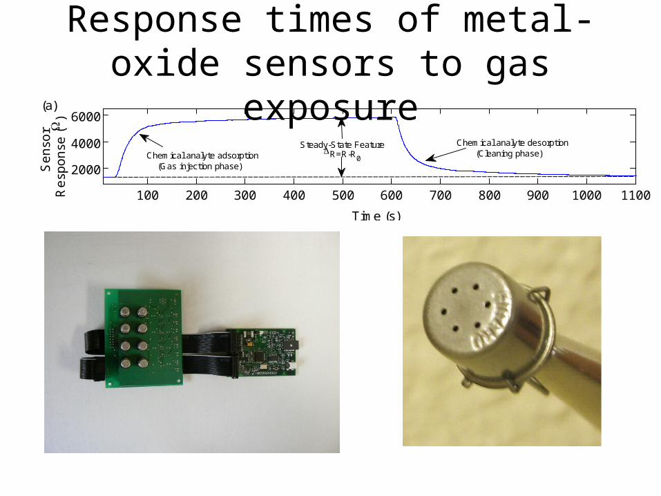
(a)

Chemical analyte adsorption (Gas injection phase)

Chemical analyte desorption (Cleaning phase)

max ema=0.1

max ema=0.01

Maximum values of the ema

max ema=0.001

min ema=0.1

min ema=0.01

(f)

min ema=0.001

Minimum values of the ema

(e)

(g)(d)

(b)

(c)

Steady-State FeatureR=R-R

0

100 200 300 400 500 600 700 800 900 1000 1100

2000

4000

6000

Se

nso

r

Re

spo

nse

()

100 200 300 400 500-1

0

1

em

a max

=

0.00

1

Features considered in the rising portionof the sensor response

100 200 300 400 500-2

0

2

em

a max

=

0.01

600 700 800 900 1000 1100-1

0

1

Features considered in the decaying portionof the sensor response

em

a min

=

0.00

1

600 700 800 900 1000 1100-2

0

2

em

a min

=

0.01

600 700 800 900 1000 1100-2

0

2

Time (s)

em

a min

=

0.1

100 200 300 400 500-2

0

2

em

a max

=

0.1

(a)

Chemical analyte adsorption (Gas injection phase)

Chemical analyte desorption (Cleaning phase)

max ema=0.1

max ema=0.01

Maximum values of the ema

max ema=0.001

min ema=0.1

min ema=0.01

(f)

min ema=0.001

Minimum values of the ema

(e)

(g)(d)

(b)

(c)

Steady-State FeatureR=R-R

0

Response times of metal-oxide sensors to gas exposure

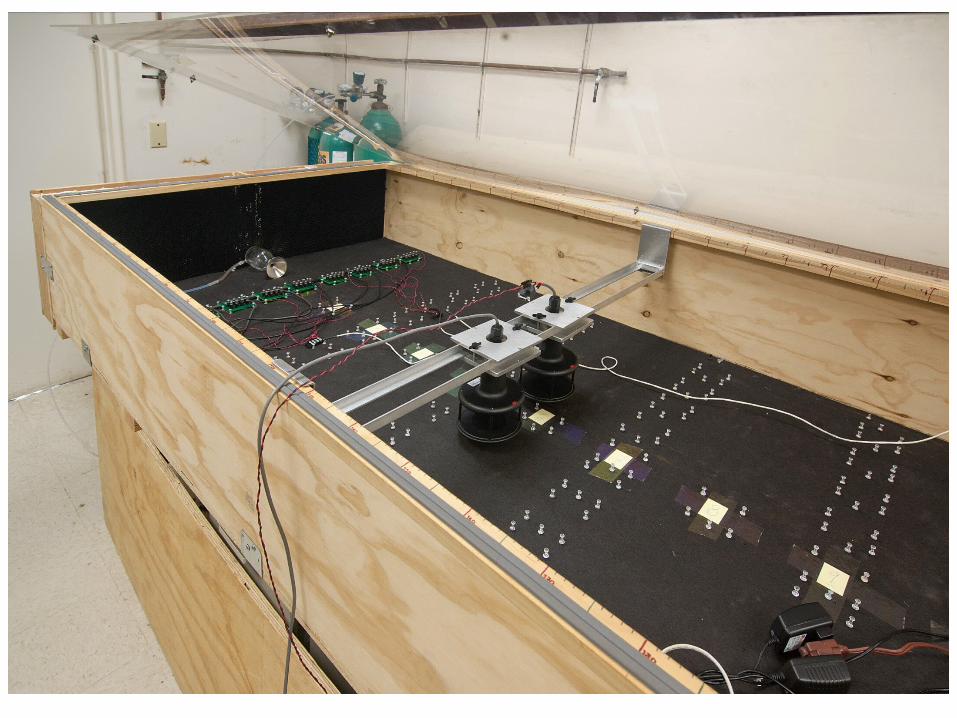
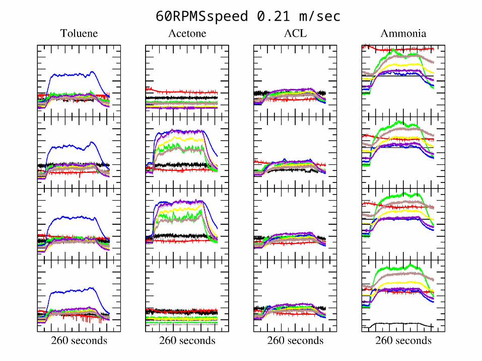
60RPMSspeed 0.21 m/sec

Fig. 7 Average accuracy of the models trained in one position landmark and validated in the rest of the positions. The models are trained and validated at the same sensors’ temperature and wind speed. Models trained in position lines # 1 and # 2 show poor ...

Alexander Vergara , Jordi Fonollosa , Jonas Mahiques , Marco Trincavelli , Nikolai Rulkov , Ramón Huerta

Sensors and Actuators B: Chemical, Volume 185, 2013, 462 - 477

http://dx.doi.org/10.1016/j.snb.2013.05.027

Sen

sor

resp

onse

Feature # / Sensor feature/ “Olfactory receptor”

ORN type

Evo

ked

Spi

ke R

ate

ORN population response (24 of 51 ORN types) to a single odor

Hallem and Carlson Cell 2005

Sensory neuron representations

Main computational tasks

• Classification: What is the machinery used for gas discrimination?

• Regression: How do they estimate gas concentration or distance to the source?

Feature Extraction:Spatio-temporal coding

High divergence-convergence ratiosfrom layer to layer.

Antennal Lobe (AL) Mushroom body (MB)

Antenna

Main location of learning

The simplified insect brain: model 0

Sparse code

Output neurons

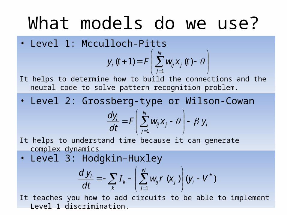
What models do we use?• Level 1: Mcculloch-Pitts

It helps to determine how to build the connections and the neural code to solve pattern recognition problem.

N

jjiji txwFty

1

)()1(

• Level 3: Hodgkin–Huxley

It teaches you how to add circuits to be able to implement Level 1 discrimination.

ki

N

jjijk

i VyxrwIdt

yd)()( *

1

• Level 2: Grossberg-type or Wilson-Cowan

It helps to understand time because it can generate complex dynamics

i

N

jjij

i yxwFdt

dy

1

PNs (2%) iKC(35%) Output(0.1%)

AL No learningrequired

Stage I: Transformation into a large display

Stage II: Learning “perception” of odors

CALYX

Display Layer

Kenyon Cells

MB lobes

Decision layer

Output neurons

Sparsecode

Sparsecode

InhibitionInhibition

HebbianplasticityHebbianplasticity

Fan-out systems

• PROS or CONS: What do you want to know first?

The inherent instability of the fan-out structure

ALN

jjiji txcFty

1

)()1(

Fan-out: solvable inconveniences

• The Projection from the PNs to KCs amplify noise.

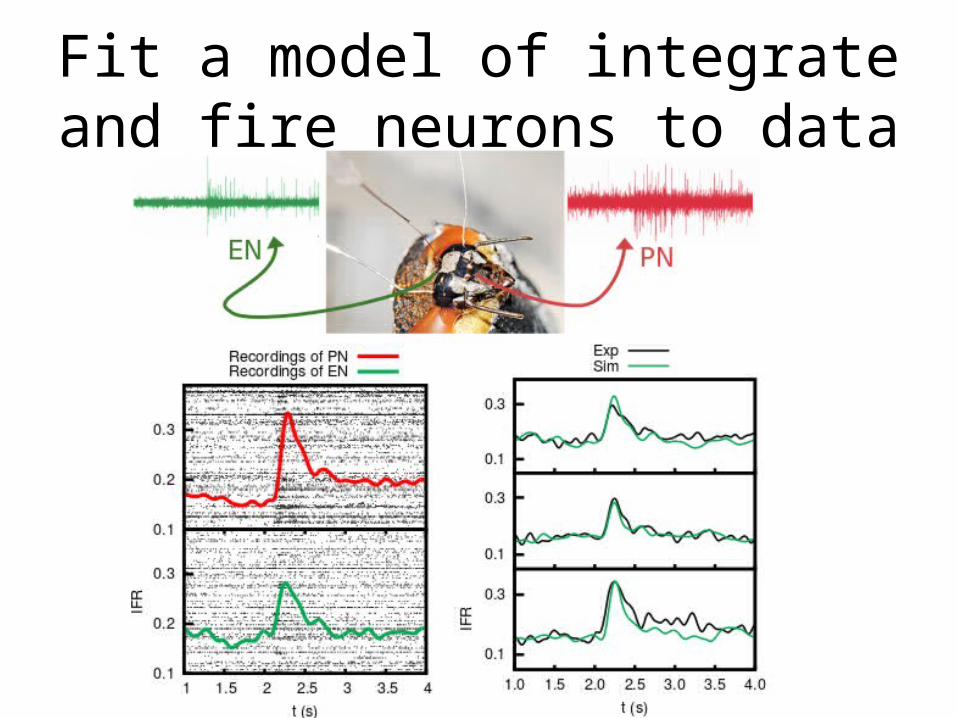
Fit a model of integrate and fire neurons to data

Main message of the cons

• Fan-out systems amplify everything even the bad stuff.

• Gain control or gain modulation systems are needed if one wants to use them.

PROS!

Classification is easier in higher dimensions

ALN

jjiji txcFty

1

)()1(

O

N

jjiji

KC

tywFtz 1

)1()2(

Linear versus nonlinear classifiers?Fernández-Delgado, M., Cernadas, E., Barro, S., & Amorim, D. (2014). Do we need hundreds of classifiers to solve real world classification problems?. The Journal of Machine Learning Research, 15(1), 3133-3181.

• The authors evaluate 179 classifiers arising from 17 families (discriminant analysis, Bayesian, neural networks, support vector machines, decision trees, rule-based classifiers, boosting, bagging, stacking, random forests and other ensembles, generalized linear models, nearest neighbors, partial least squares and principal component regression, logistic and multinomial regression, multiple adaptive regression splines and other methods).

• The authors use 121 data sets, which represent the whole UCI data base (excluding the large-scale problems) and other own real problems, in order to achieve

• The classifiers most likely to be the bests are the random forest (RF) versions, the best of which achieves 94.1% of the maximum accuracy overcoming 90% in the 84.3% of the data sets. The SVM with Gaussian kernel achieves 92.3% of the maximum accuracy.

What are the best known classification methods?

32.9 82.0 parRF t (RF) 33.1 82.3 rf t (RF) 36.8 81.8 svm C (SVM) 38.0 81.2 svmPoly t (SVM) 39.4 81.9 rforest R (RF) 39.6 82.0 elm kernel m (NNET) 40.3 81.4 svmRadialCost t (SVM)42.5 81.0 svmRadial t (SVM)

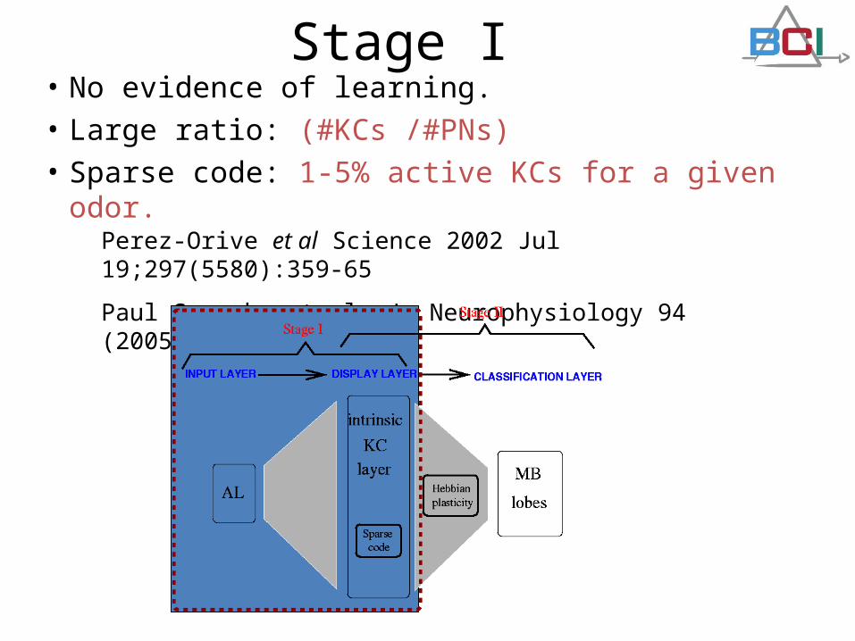
• No evidence of learning.• Large ratio: (#KCs /#PNs)• Sparse code: 1-5% active KCs for a given odor.

Stage I

Perez-Orive et al Science 2002 Jul 19;297(5580):359-65

Paul Szyszka et al, J. Neurophysiology 94 (2005).

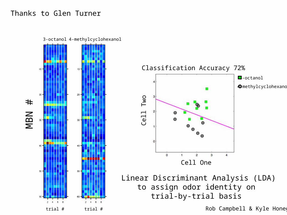
3-octanol 4-methylcyclohexanol

trial #trial #

MB

N #

Linear Discriminant Analysis (LDA)to assign odor identity on

trial-by-trial basis

Cell One

Cel

l Tw

o

3-octanol

4-methylcyclohexanol

Classification Accuracy 72%

Rob Campbell & Kyle Honegger

Thanks to Glen Turner

Evidence of learning in the MB: Heisenberg et al (1985) J Neurogenet 2 , pp. 1-30.

Mauelshagen J. (1993) J Neurophysiol. 69(2):609-25.Belle and Heisenberg,(1994) Science 263 , pp. 692-695. Connolly et al (1996) Science 274 (5295): 2104Zars et al (2000) Science 288(5466):672-5.Pascual and Preat (2001) Science 294(5544):1115-7. Dubnau et al (2001) Nature 411(6836):476-80.Menzel & Manz (2005) J. Experimental Biol. 208: 4317-4332Okada, Rybak, &Menzel (2007) J. of Neuroscience 27(43): 11736-47Stijn Cassenaer &Laurent (2007) Nature 448:709-713.Strube-Bloss MF, Nawrot MP and Menzel R (2011): Mushroom Body Output Neurons Encode Odor-Reward Association. The Journal of Neuroscience, 31(8): 3129-3140

Key elements:1. Hebbian plasticity in w.

2. Competition via inhibition (gain control).

LN1

LN2

Thanks to Stijn Cassenaer

So what about the inhibition?

rest

ePwitheRzytwtw ij

ijij

0

)(2

1sgn

)()1(

)(eR +1 positive reward and -1 negative reward

So, what about the plasticity? Hebbian rule

(Dehaene, Changeux, 2000) and (Houk, Adams, Barto 1995)

Ventral Unpaired Median cell mx1 (VUMmx1)

VUMmx1responds to Sucrose application to the proboscis and/or antennae

sucrose

Receives input from gustatory input regions

Broadly aroborizes brain regions associated with olfactory processing, sensory integration and premotor areas

So, what about the reinforcement?

Another Advantage

• Robustness

MB performance on MNIST dataset

•Huerta R, Nowotny T, Fast and robust learning by reinforcement signals: explorations in the insect brain. Neural Comput. 2009 Aug;21(8):2123-51.

Testing MB resilience on MNIST dataset

Proboscis extension

Retraction

Kenyon cells

Output neurons

Sucrose

Sucrose

Active Kenyon cell

ExtensionActive

RetractionActive

+

-

Sucrose

Active Kenyon cell

ExtensionActive

RetractionInactive

+

Option 1

Option 2

Bazhenov, Maxim, Ramon Huerta, and Brian H. Smith. "A computational framework for understanding decision making through integration of basic learning rules." The Journal of Neuroscience 33.13 (2013): 5686-5697.

Analogy with machine learning devices: Support Vector Machines (SVM)

• Given a training set

]1,1[,,,,1},,{ iM

iii yxNiyx

Odorant in the AL coding space

Good or bad? How many samples?

Good Bad

SVM• SVMs often use a expansion function (a Calyx)

with the feature space (the KC neural coding space).

,:)( M

• The classification function, the odor recognition function or the pattern recognition function is

)(,)( ii wf

The output neurons, the β-lobe neurons, or the extrinsic neurons

The output neurons, the β-lobe neurons, or the extrinsic neurons

The connections from the Calyx to the output neurons. what we are trying to learn.

The connections from the Calyx to the output neurons. what we are trying to learn.

The Calyx neural codingThe Calyx neural coding

The AL neural codingThe AL neural coding

CALYX

Display Layer

IntrinsicKenyon Cells

AL

MB lobes

Decision layer

ExtrinsicNeurons

Competition Viainhibition

codingAL,)( )(,)( ii wf

w

SVM• We want to solve the classification problem:

N

iiiw yfCw

1

2)0,)(1max(

2

1min

Minimize the strength of the connections

Minimize the errors

SVM stochastic gradient algorithm

correctstrongly 0

incorrrectalmost )( ii yCww

Make the connections as small as possible

Change the connections if the sample is not correctly classified

Connection removal is necessary to generalize better. To avoid overfitting.

rest

ePwitheRfxw ijij

0

)()(Hebbian

Remarkable similarities1. Structural organization: AL->Calyx ->ML Lobes2. Connection removal and Hebbian learning:

Perceptron rule3. Inhibition provides robustness and allow to learn

from fewer examples better.

1. Structural organization: AL->Calyx ->ML Lobes2. Connection removal and Hebbian learning:

Perceptron rule3. Inhibition provides robustness and allow to learn

from fewer examples better.

Kerem Muezzinoglu(UCSD-Biocircuits, now )Alex Vergara (UCSD-Biocircuits)Shankar Vembu(UCSD-Biocircuits)Thomas Nowotny(Sussex, UK)Amy Ryan (JPL-NASA)Margie Homer (JPL-NASA)Brian Smith (ASU)Gilles Laurent (CALTECH-Max Planck)Nikolai Rulkov (UCSD-Biocirucits)Mikhail Rabinovich (UCSD-Biocircuits)Travis Wong (ELINTRIX, San Diego)Drew Barnett (ELINTIRX, San Diego)Marco Trincavelli (Orebro, Sweden)Pablo Varona (UAM, Spain)Francisco Rodriguez (UAM, Spain)Marta Garcia Sanchez (UAM, Spain)

Thank you!