ARTICLE IN PRESS

Contents lists available at ScienceDirect

Int. J. Production Economics

Int. J. Production Economics 120 (2009) 115–124

0925-52

doi:10.1

� Cor

E-m

journal homepage: www.elsevier.com/locate/ijpe

The production, remanufacture and waste disposal modelwith lost sales

Mohamad Y. Jaber �, Ahmed M.A. El Saadany

Department of Mechanical and Industrial Engineering, Ryerson University, Toronto, ON, Canada M5B 2K3

a r t i c l e i n f o

Article history:

Received 1 September 2007

Accepted 1 July 2008Available online 17 October 2008

Keywords:

Production

EOQ model

Remanufacturing (repair)

Waste disposal

Lost sales

73/$ - see front matter & 2008 Elsevier B.V. A

016/j.ijpe.2008.07.016

responding author. Tel.: +416 979 5000x7623;

ail address: mjaber@ryerson.ca (M.Y. Jaber).

a b s t r a c t

Inventory management in reverse logistics has been receiving increasing attention in

recent years. One of the inventory problems that has been of interest to researchers is

the production, remanufacture (repair) and waste disposal model, where used items are

collected and remanufactured to ‘‘as-good-as new’’ state. The available models in the

literature assume that customers’ demand is satisfied from newly manufactured

(produced) items and from remanufactured (repaired) items. This may be true in few

industries, but not in other industries where customers do not consider ‘‘new’’

(‘‘manufactured’’) and ‘‘remanufactured’’ (‘‘repaired’’) items as being interchangeable.

This paper extends along this line of research and assumes that demand for

manufactured items is different from that for remanufactured (repaired) ones. This

assumption results in lost sales situations where there are stock-out periods for

manufactured and remanufactured items. Mathematical models are developed and

numerical examples provided with results discussed.

& 2008 Elsevier B.V. All rights reserved.

1. Introduction

Reverse logistics gave rise to the drive towardscollecting and remanufacturing used products to extendtheir useable lives and thus reduce waste and conservenatural resources; with remanufacturing being a collec-tive noun for processes such as repairing, reusing,refurbishing or recycling of products reaching theireconomic and/or end lives. Like supply chains, reverselogistics manage the flow of returned used products forremanufacturing or repairing or other purposes; however,in the opposite direction (i.e., from downstream toupstream), and therefore managing inventory in reverselogistics has been stressed in several studies (e.g.,Fleischmann et al., 1997; Minner, 2003).

Although reverse logistics is relatively a new businessterm, initial attempts to address the inventory of repaired

ll rights reserved.

fax: +416 979 5265.

items or products dates back to the 1960s. The firstreported work is that of Schrady (1967) who developed anEOQ model for repaired items where production andrepair rates are instantaneous with no disposal cost. Thework of Schrady has been extended by assuming a finiterepair rate (Nahmias and Rivera, 1979) and a multi-product case (Mabini et al., 1992).

As reverse logistics came to be a business term in the1990s, the research of the inventory and remanufacturingproblem took a new trend. Richter (1996a, b) investigatedthe EOQ model for stationary demand that is satisfiedfrom producing items of a certain product using newmaterial and components, and from repairing used itemsthat are collected from the market at some rate. In follow-up works, Richter (1997) and Richter and Dobos (1999)showed that a pure policy of either no waste disposal(total repair) or no repair (total waste disposal) is alwaysoptimal. Dobos and Richter (2003) investigated a produc-tion/recycling system with constant demand that issatisfied by non-instantaneous production and recyclingwith a single repair and a single production cycles per

ARTICLE IN PRESS

M.Y. Jaber, A.M.A. El Saadany / Int. J. Production Economics 120 (2009) 115–124116

time interval. In a subsequent paper, Dobos and Richter(2004) generalized their earlier model (Dobos and Richter,2003) to the case of multiple repair and production cycles.Recently, and along the same line of research, Dobosand Richter (2006) extended their previous work andassumed that the quality of collected used/returned itemsis not always suitable for further recycling, i.e. not allused/returned items can be reused.

Like Richter, Teunter has been researching along thesame line, but with different assumptions. Teunter (2001)extended the work of Schrady (1967) by considering morethan one production cycle and several repair cycles. In asubsequent paper, Teunter (2002) extended his earlierwork by considering discounted cost inventory systemwith stochastic demand and return where the lead-timesfor manufacturing and remanufacturing are negligible. Ina recent article, Teunter (2004) derived closed formexpressions to determine the optimal lot sizes for theproduction/procurement of new items and for the recov-ery/repair of returned items. Other researchers have alsodeveloped models along the same lines as Schrady,Richter, and Teunter, but with different assumptions.These works are, but not limited to, those of Inderfurthet al. (2005), Konstantaras and Papachristos (2006, 2007),Buscher and Lindner (2007), Choi et al. (2007), El Saadanyand Jaber (2008), and Jaber and Rosen (2008).

The above surveyed works assumed customer demandis satisfied from a stock of serviceable (manufacturedand remanufactured) items. In general, customers do notconsider newly manufactured (used interchangeably withthe word produced) items and remanufacture (repaired)ones as being interchangeable. Remanufactured goods sellat lower price points in secondary markets, or in differentchannels than new products that sell in primary markets.See for instance the works of Tibben-Lembke and Rogers(2002) and Blackburn et al. (2004). This paper extends thework of Richter (1996a, b) by assuming that demand formanufactured items is different from that for remanufac-tured (repaired) ones. This assumption results in lost salessituations where there are stock-out periods for manu-factured and remanufactured items, i.e., demand fornewly manufactured items is lost during remanufacturingcycles and vice versa.

The remainder of this paper is organized as follows.The next section, Section 2, presents the assumptions andnotations. Section 3 is for mathematical modelling.Section 4 is for numerical examples and discussion ofresults. Finally, the paper summarizes and concludes inSection 5.

2. Assumptions and notations

2.1. Assumptions

This paper assumes: (1) a single-product case with twodifferent qualities, (2) infinite production and recoveryrates, (3) remanufactured items are perceived by somecustomers to be of lower quality than newly manufac-tured items, (4) demand for produced and remanufac-tured items are known, constant but different, (5)

constant but different collection rates for previously usedmanufactured and remanufactured items, (6) lead timeis zero, (7) inventory stock-out occurs and unsatisfieddemand (manufactured or remanufactured) is lost, (8)unlimited storage capacity is available, and (9) infiniteplanning horizon. Furthermore, this paper assumes thatthe collection of used items from previously remanufac-tured ones occur in the remanufacturing period. Likewise,used items from previously produced items occur duringthe production period.

2.2. Notations

Decision variables:

n number of production cycles in an interval oflength T.

m number of remanufacturing cycles in an intervalof length T.

gp collection percentage of available returns ofnewly produced items (0ogpo1).

gr collection percentage of available returns ofpreviously remanufactured items (0ogro1).

Input parameters:

Dp demand rate for newly produced items (units/unit of time).

Dr demand rate for remanufactured items (units/unit of time), where Dr is not necessarily equalto Dp

Sp setup cost for a production cycle ($).Sr setup cost for a remanufacturing cycle ($).hp holding cost per unit per unit of time of a

produced item ($/unit/unit of time).hr holding cost per unit per unit of time of a

remanufactured item ($/unit/unit of time).hu holding cost per unit per unit of time of a used

item ($/unit/unit of time).cp cost per unit of a lost demand for a produced

item ($/unit).cr cost per unit of a lost demand for a remanu-

factured item ($/unit).bp percentage of available returns from the primary

market for produced items.br percentage of available returns from the

secondary market for remanufactured items(0obrpbpo1). Note that 1�br and 1�bp arethe waste disposal rates.

Decision variables dependent parameters

x2 lot size quantity (in units) to be remanufactured/repaired in an interval of length T.

x1 lot size quantity (in units) to be produced in aninterval of length T.

Tp length of a production interval (units of time),where Tp ¼ x1/Dp.

ARTICLE IN PRESS

M.Y. Jaber, A.M.A. El Saadany / Int. J. Production Economics 120 (2009) 115–124 117

Tr length of a remanufacturing interval (units oftime), where Tr ¼ x2/Dr.

T interval length (units of time), where T ¼ Tr+Tp.

It is reasonable to assume that it is less likely to recovercomponents from a used item that was previouslyremanufactured than from a previously produced one,and therefore, this paper assumes brpbp.

3. Mathematical modelling

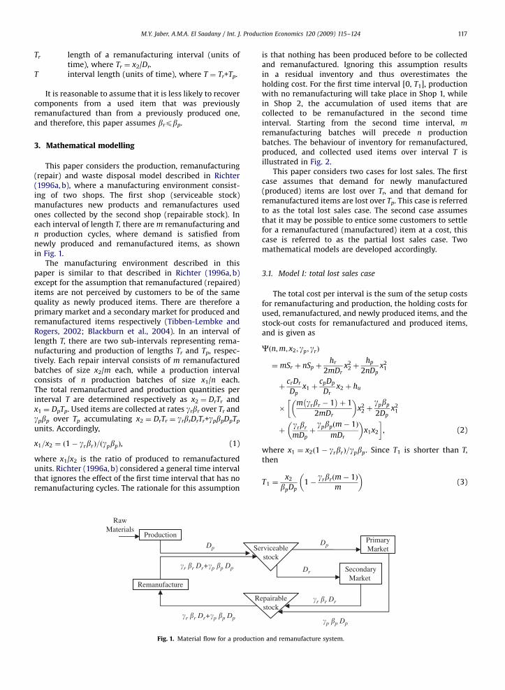
This paper considers the production, remanufacturing(repair) and waste disposal model described in Richter(1996a, b), where a manufacturing environment consist-ing of two shops. The first shop (serviceable stock)manufactures new products and remanufactures usedones collected by the second shop (repairable stock). Ineach interval of length T, there are m remanufacturing andn production cycles, where demand is satisfied fromnewly produced and remanufactured items, as shownin Fig. 1.

The manufacturing environment described in thispaper is similar to that described in Richter (1996a, b)except for the assumption that remanufactured (repaired)items are not perceived by customers to be of the samequality as newly produced items. There are therefore aprimary market and a secondary market for produced andremanufactured items respectively (Tibben-Lembke andRogers, 2002; Blackburn et al., 2004). In an interval oflength T, there are two sub-intervals representing rema-nufacturing and production of lengths Tr and Tp, respec-tively. Each repair interval consists of m remanufacturedbatches of size x2/m each, while a production intervalconsists of n production batches of size x1/n each.The total remanufactured and production quantities perinterval T are determined respectively as x2 ¼ DrTr andx1 ¼ DpTp. Used items are collected at rates grbr over Tr andgpbp over Tp accumulating x2 ¼ DrTr ¼ grbrDrTr+gpbpDpTp

units. Accordingly,

x1=x2 ¼ ð1� grbrÞ=ðgpbpÞ, (1)

where x1/x2 is the ratio of produced to remanufacturedunits. Richter (1996a, b) considered a general time intervalthat ignores the effect of the first time interval that has noremanufacturing cycles. The rationale for this assumption

Production

Remanufacture

R

RawMaterials

SeDp

�r �r Dr+�p �p Dp

�r �r Dr+�p �p Dp

Fig. 1. Material flow for a productio

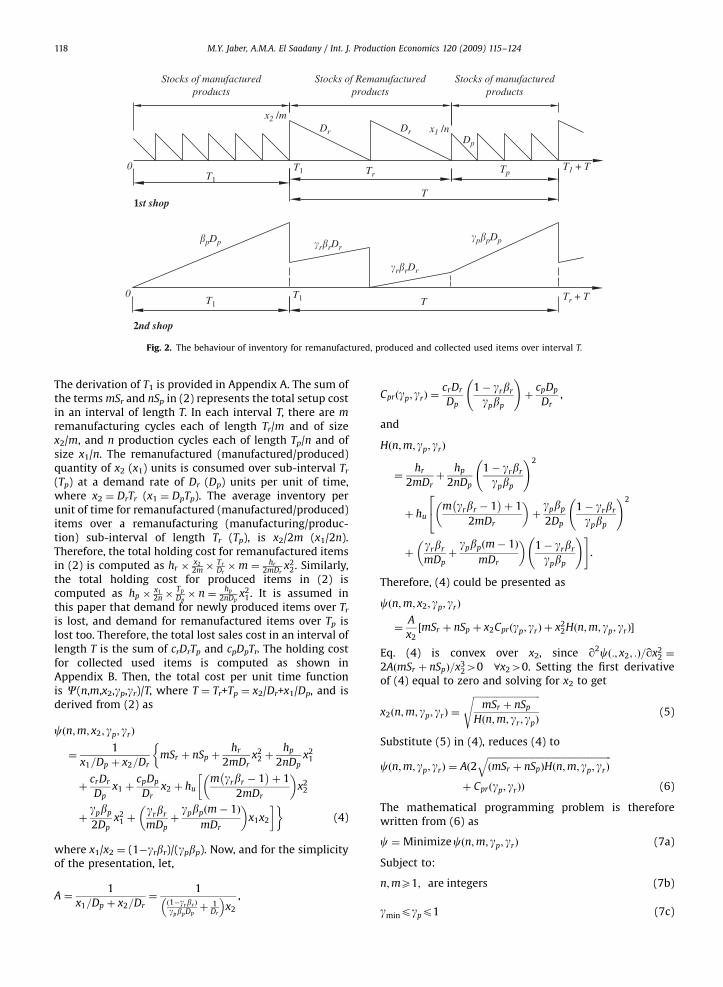
is that nothing has been produced before to be collectedand remanufactured. Ignoring this assumption resultsin a residual inventory and thus overestimates theholding cost. For the first time interval [0, T1], productionwith no remanufacturing will take place in Shop 1, whilein Shop 2, the accumulation of used items that arecollected to be remanufactured in the second timeinterval. Starting from the second time interval, m

remanufacturing batches will precede n productionbatches. The behaviour of inventory for remanufactured,produced, and collected used items over interval T isillustrated in Fig. 2.

This paper considers two cases for lost sales. The firstcase assumes that demand for newly manufactured(produced) items are lost over Tr, and that demand forremanufactured items are lost over Tp. This case is referredto as the total lost sales case. The second case assumesthat it may be possible to entice some customers to settlefor a remanufactured (manufactured) item at a cost, thiscase is referred to as the partial lost sales case. Twomathematical models are developed accordingly.

3.1. Model I: total lost sales case

The total cost per interval is the sum of the setup costsfor remanufacturing and production, the holding costs forused, remanufactured, and newly produced items, and thestock-out costs for remanufactured and produced items,and is given as

Cðn;m; x2; gp; grÞ

¼ mSr þ nSp þhr

2mDrx2

2 þhp

2nDpx2

1

þcrDr

Dpx1 þ

cpDp

Drx2 þ hu

�m grbr � 1� �

þ 1

2mDr

� �x2

2 þgpbp

2Dpx2

1

�

þgrbr

mDpþgpbp m� 1ð Þ

mDr

� �x1x2

�, (2)

where x1 ¼ x2ð1� grbrÞ=gpbp. Since T1 is shorter than T,then

T1 ¼x2

bpDp1�

grbrðm� 1Þ

m

� �(3)

SecondaryMarket

epairablestock

Dr

PrimaryMarketrviceable

stock

Dp

�r �r Dr

�p �p Dp

n and remanufacture system.

ARTICLE IN PRESS

1st shop

2nd shop

Stocks of manufacturedproducts

Stocks of Remanufacturedproducts

T

Stocks of manufacturedproducts

0 T1

0 T1T1

T1 T

T1 + T

x2 /mx1 /nDr Dr

Dp

Tr Tp

Tr + T

�pDp

�r�rDr

�r�rDr�p�pDp

Fig. 2. The behaviour of inventory for remanufactured, produced and collected used items over interval T.

M.Y. Jaber, A.M.A. El Saadany / Int. J. Production Economics 120 (2009) 115–124118

The derivation of T1 is provided in Appendix A. The sum ofthe terms mSr and nSp in (2) represents the total setup costin an interval of length T. In each interval T, there are m

remanufacturing cycles each of length Tr/m and of sizex2/m, and n production cycles each of length Tp/n and ofsize x1/n. The remanufactured (manufactured/produced)quantity of x2 (x1) units is consumed over sub-interval Tr

(Tp) at a demand rate of Dr (Dp) units per unit of time,where x2 ¼ DrTr (x1 ¼ DpTp). The average inventory perunit of time for remanufactured (manufactured/produced)items over a remanufacturing (manufacturing/produc-tion) sub-interval of length Tr (Tp), is x2/2m (x1/2n).Therefore, the total holding cost for remanufactured itemsin (2) is computed as hr �

x22m�

Tr

Dr�m ¼ hr

2mDrx2

2. Similarly,the total holding cost for produced items in (2) iscomputed as hp �

x12n�

Tp

Dp� n ¼ hp

2nDpx2

1. It is assumed inthis paper that demand for newly produced items over Tr

is lost, and demand for remanufactured items over Tp islost too. Therefore, the total lost sales cost in an interval oflength T is the sum of crDrTp and cpDpTr. The holding costfor collected used items is computed as shown inAppendix B. Then, the total cost per unit time functionis C(n,m,x2,gp,gr)/T, where T ¼ Tr+Tp ¼ x2/Dr+x1/Dp, and isderived from (2) as

cðn;m; x2; gp; grÞ

¼1

x1=Dp þ x2=DrmSr þ nSp þ

hr

2mDrx2

2 þhp

2nDpx2

1

�

þcrDr

Dpx1 þ

cpDp

Drx2 þ hu

m grbr � 1� �

þ 1

2mDr

� �x2

2

�

þgpbp

2Dpx2

1 þgrbr

mDpþgpbp m� 1ð Þ

mDr

� �x1x2

�(4)

where x1/x2 ¼ (1�grbr)/(gpbp). Now, and for the simplicityof the presentation, let,

A ¼1

x1=Dp þ x2=Dr¼

1ð1�grbr Þ

gpbpDpþ 1

Dr

�x2

,

Cprðgp; grÞ ¼crDr

Dp

1� grbr

gpbp

!þ

cpDp

Dr,

and

Hðn;m; gp; grÞ

¼hr

2mDrþ

hp

2nDp

1� grbr

gpbp

!2

þ hum grbr � 1� �

þ 1

2mDr

� �þgpbp

2Dp

1� grbr

gpbp

!224

þgrbr

mDpþgpbp m� 1ð Þ

mDr

� �1� grbr

gpbp

!#.

Therefore, (4) could be presented as

cðn;m; x2; gp; grÞ

¼A

x2½mSr þ nSp þ x2Cprðgp; grÞ þ x2

2Hðn;m; gp; grÞ�

Eq. (4) is convex over x2, since q2cð:; x2; :Þ=qx22 ¼

2AðmSr þ nSpÞ=x3240 8x240. Setting the first derivative

of (4) equal to zero and solving for x2 to get

x2ðn;m; gp; grÞ ¼

ffiffiffiffiffiffiffiffiffiffiffiffiffiffiffiffiffiffiffiffiffiffiffiffiffiffiffiffiffimSr þ nSp

Hðn;m; gr ; gpÞ

s(5)

Substitute (5) in (4), reduces (4) to

cðn;m; gp; grÞ ¼ Að2ffiffiffiffiffiffiffiffiffiffiffiffiffiffiffiffiffiffiffiffiffiffiffiffiffiffiffiffiffiffiffiffiffiffiffiffiffiffiffiffiffiffiffiffiffiffiffiffiffiffiffiffiffiffiðmSr þ nSpÞHðn;m; gp; grÞ

qþ Cprðgp; grÞÞ (6)

The mathematical programming problem is thereforewritten from (6) as

c ¼Minimizecðn;m; gp; grÞ (7a)

Subject to:

n;mX1; are integers (7b)

gminpgpp1 (7c)

ARTICLE IN PRESS

M.Y. Jaber, A.M.A. El Saadany / Int. J. Production Economics 120 (2009) 115–124 119

0pgrp1 (7d)

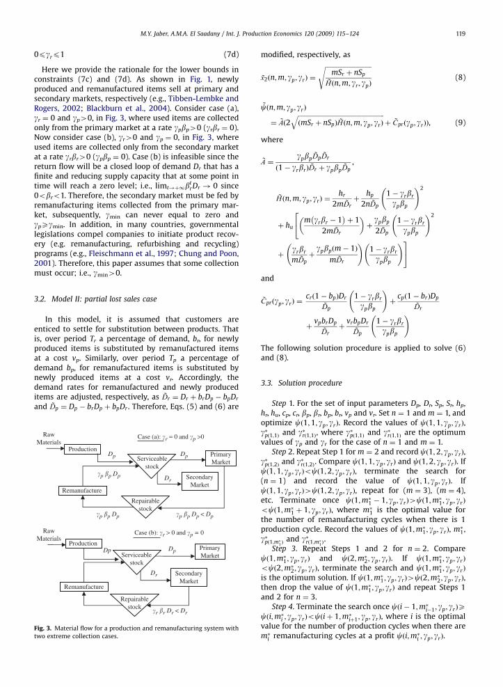
Here we provide the rationale for the lower bounds inconstraints (7c) and (7d). As shown in Fig. 1, newlyproduced and remanufactured items sell at primary andsecondary markets, respectively (e.g., Tibben-Lembke andRogers, 2002; Blackburn et al., 2004). Consider case (a),gr ¼ 0 and gp40, in Fig. 3, where used items are collectedonly from the primary market at a rate gpbp40 (grbr ¼ 0).Now consider case (b), gr40 and gp ¼ 0, in Fig. 3, whereused items are collected only from the secondary marketat a rate grbr40 (gpbp ¼ 0). Case (b) is infeasible since thereturn flow will be a closed loop of demand Dr that has afinite and reducing supply capacity that at some point intime will reach a zero level; i.e., limt!þ1b

trDr ! 0 since

0obro1. Therefore, the secondary market must be fed byremanufacturing items collected from the primary mar-ket, subsequently, gmin can never equal to zero andgpXgmin. In addition, in many countries, governmentallegislations compel companies to initiate product recov-ery (e.g. remanufacturing, refurbishing and recycling)programs (e.g., Fleischmann et al., 1997; Chung and Poon,2001). Therefore, this paper assumes that some collectionmust occur; i.e., gmin40.

3.2. Model II: partial lost sales case

In this model, it is assumed that customers areenticed to settle for substitution between products. Thatis, over period Tr a percentage of demand, br, for newlyproduced items is substituted by remanufactured itemsat a cost vp. Similarly, over period Tp a percentage ofdemand bp, for remanufactured items is substituted bynewly produced items at a cost vr. Accordingly, thedemand rates for remanufactured and newly produceditems are adjusted, respectively, as Dr ¼ Dr þ brDp � bpDr

and Dp ¼ Dp � brDp þ bpDr . Therefore, Eqs. (5) and (6) are

RawMaterials

Production

Remanufacture

Repairablestock

Serviceable stock

Dp

RawMaterials

�p �p Dp < Dp

�r �r Dr < Dr

�p �p Dp

�p �p Dp

Production

Remanufacture

SecondaryMarket

Repairablestock

Dr

PrimaryMarket

SecondaryMarket

PrimaryMarket

Serviceablestock

Dp Dp

Dr

Dp

Case (a): �r = 0 and �p >0

Case (b): �r > 0 and �p = 0

Fig. 3. Material flow for a production and remanufacturing system with

two extreme collection cases.

modified, respectively, as

x2ðn;m; gp; grÞ ¼

ffiffiffiffiffiffiffiffiffiffiffiffiffiffiffiffiffiffiffiffiffiffiffiffiffiffiffiffiffimSr þ nSp

Hðn;m; gr ; gpÞ

s(8)

cðn;m; gp; grÞ

¼ Að2ffiffiffiffiffiffiffiffiffiffiffiffiffiffiffiffiffiffiffiffiffiffiffiffiffiffiffiffiffiffiffiffiffiffiffiffiffiffiffiffiffiffiffiffiffiffiffiffiffiffiffiffiffiffiðmSr þ nSpÞHðn;m; gp; grÞ

qþ Cprðgp; grÞÞ, (9)

where

A ¼gpbpDpDr

ð1� grbrÞDr þ gpbpDp

,

Hðn;m; gp; grÞ ¼hr

2mDrþ

hp

2nDp

1� grbr

gpbp

!2

þ hum grbr � 1� �

þ 1

2mDr

� �þgpbp

2Dp

1� grbr

gpbp

!224

þgrbr

mDpþgpbp m� 1ð Þ

mDr

!1� grbr

gpbp

!35and

Cprðgp; grÞ ¼crð1� bpÞDr

Dp

1� grbr

gpbp

!þ

cpð1� brÞDp

Dr

þvpbrDp

Dr

þvrbpDr

Dp

1� grbr

gpbp

!

The following solution procedure is applied to solve (6)and (8).

3.3. Solution procedure

Step 1. For the set of input parameters Dp, Dr, Sp, Sr, hp,hr, hu, cp, cr, bp, br, bp, br, vp and vr. Set n ¼ 1 and m ¼ 1, andoptimize cð1;1; gp; grÞ. Record the values of cð1;1; gp; grÞ,g�pð1;1Þ and g�rð1;1Þ, where g�pð1;1Þ and g�rð1;1Þ are the optimumvalues of gp and gr for the case of n ¼ 1 and m ¼ 1.

Step 2. Repeat Step 1 for m ¼ 2 and record cð1;2; gp; grÞ,g�pð1;2Þ and g�rð1;2Þ. Compare cð1;1; gp; grÞ and cð1;2; gp; grÞ. Ifcð1;1; gp; grÞocð1;2; gp; grÞ, terminate the search for(n ¼ 1) and record the value of cð1;1; gp; grÞ. Ifcð1;1; gp; grÞ4cð1;2; gp; grÞ, repeat for (m ¼ 3), (m ¼ 4),etc. Terminate once cð1;m�1 � 1; gp; grÞ4cð1;m�1; gp; grÞ

ocð1;m�1 þ 1; gp; grÞ, where m�1 is the optimal value forthe number of remanufacturing cycles when there is 1production cycle. Record the values of cð1;m�1; gp; grÞ, m�1,g�pð1;m�

1Þ

and g�rð1;m�1Þ.

Step 3. Repeat Steps 1 and 2 for n ¼ 2. Comparecð1;m�1; gp; grÞ and cð2;m�2; gp; grÞ. If cð1;m�1; gp; grÞ

ocð2;m�2; gp; grÞ, terminate the search and cð1;m�1; gp; grÞ

is the optimum solution. If cð1;m�1; gp; grÞ4cð2;m�2; gp; grÞ,then drop the value of cð1;m�1; gp; grÞ and repeat Steps 1and 2 for n ¼ 3.

Step 4. Terminate the search once cði� 1;m�i�1; gp; grÞX

cði;m�i ; gp; grÞocðiþ 1;m�iþ1; gp; grÞ, where i is the optimalvalue for the number of production cycles when there arem�i remanufacturing cycles at a profit cði;m�i ; gp; grÞ.

ARTICLE IN PRESS

M.Y. Jaber, A.M.A. El Saadany / Int. J. Production Economics 120 (2009) 115–124120

4. Numerical results

In this section, several numerical examples are solvedwhose parameters were collected from the availableliterature. Three numerical examples were selected fromDobos and Richter (2003), Dobos and Richter (2004) andTeunter (2004). Note that these studies, like other studiesin the literature, assumed that the remanufactured itemsare as-good-as-new, i.e., D ¼ Dp ¼ Dr and b ¼ bp ¼ br, andthere is no need for substitution between products.Subsequently, these studies also assumed hp ¼ hr andcp ¼ cr ¼ 0. Therefore, when solving the above indi-cated numerical examples, it is necessary to assumevalues for hr, cp, cr and br. After solving these numericalexamples, a simulation study to further investigate thebehaviour of Model I was conducted where its inputparameters were randomized each over its range(of minimum and maximum values). These minimum/maximum values were determined from the abovementioned studies.

4.1. Model I

Example 1. (Dobos and Richter, 2003; p. 44): LetDp ¼ Dr ¼ 200, Sp ¼ 144, Sr ¼ 72, hp ¼ 12, hr ¼ 3, hu ¼ 3,cp ¼ 5, cr ¼ 5, and bp ¼ br ¼ 0.667. In this numerical

Table 1A numerical example illustrating the solution procedure

Trial n m gp gr

1 1 1 1 0.995

2 1 2 1 1

3 1 3 1 1

4 2 1 1 0

5 2 2 1 1

6 2 3 1 1

7 2 4 1 1

8

Table 2Optimal policies for changing values of Sr and Sp

m n gr (%)

Sr 1 14 1 100

226 1 1 100

227 1 2 0

291 1 3 0

292 1 35 0

500 1 45 0

Sp 1 1 206 0

35 1 35 0

36 1 3 0

45 1 2 0

46 1 1 100

500 3 1 100

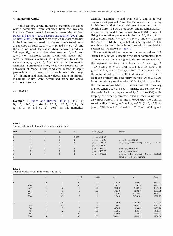
example (Example 1) and Examples 2 and 3, it wasassumed that gmin ¼ 0.01 (or 1%). The reason for assumingit this low is that the model may favour an optimalsolution closer to a pure production and no remanufactur-ing, where the model moves closer to an EPQ/EOQ model.Using the solution procedure in Section 3.3, the optimalpolicy occurs when gr ¼ 1, gp ¼ 1, m ¼ 2, and n ¼ 1, wherethe cost is 1,619.68, x2 ¼ 123.94, and x1 ¼ 61.97. Thesearch results from the solution procedure described inSection 3.3 are shown in Table 1.

The sensitivity of the model for increasing values of Sr

(from 1 to 500) while keeping the other parameters fixed

at their values was investigated. The results showed that

the optimal solution flips from gr ¼ 1 and gp ¼ 1

(1pSrp226), to gr ¼ 0 and gp ¼ 1 (227pSrp291), to

gr ¼ 0 and gp ¼ 0.01 (292pSrp500). This suggests that

the optimal policy is to collect all available used items

from the primary and secondary markets when Srp226,

from the primary market when 227pSrp291, and collect

the minimum available used items from the primary

market when 292pSrp500. Similarly, the sensitivity of

the model for increasing values of Sp (from 1 to 500) while

keeping the other parameters fixed at their values was

also investigated. The results showed that the optimal

solution flips from gr ¼ 0 and gp ¼ 0.01 (1pSpp35), to

gr ¼ 0 and gp ¼ 1 (36pSrp45), to gr ¼ 1 and gp ¼ 1

Cost (cn,m) Notes

c1,1 ¼ 1634.99

c1,2 ¼ 1619.98 c1,14c1,2, continue

c1,3 ¼ 1644.98 c1,2oc1,3, therefore m�1 ¼ 2, c1,2 ¼ 1619.98

c2,1 ¼ 1695.59

c2,2 ¼ 1678.82 c2,14c2,2 continue

c2,3 ¼ 1669.33 c2,24c2,3 continue

c2,4 ¼ 1678.82 c2,3oc2,4 therefore m�2 ¼ 3, c2,3 ¼ 1669.33

Since c1,2oc2,3, terminate

gp (%) x2 x1 cn,m

100 113.24 56.62 1372.07

100 118.72 59.36 1831.07

100 99.04 148.56 1831.96

100 132.39 198.59 1873.78

1 16.16 2423.97 1874.05

1 20.80 3120.10 1888.92

1 7.94 1191.06 1092.74

1 7.97 1195.51 1431.08

100 66.06 99.09 1435.98

100 55.55 83.32 1466.61

100 67.04 33.53 1469.34

100 209.91 104.95 1909.60

ARTICLE IN PRESS

Table 3Optimal policies for changing values of hr, hp, cr and cp

m m n gr (%) gp (%) x2 x1 cn,m

hr 3 2 1 100 100 123.94 61.96 1619.66

11.1 3 1 100 100 125.12 62.55 1767.32

11.2 1 1 0 100 44.98 67.47 1768.30

12 1 1 0 100 44.57 66.85 1775.46

hp 3 1 9 0 1 8.29 1244.22 1436.88

3.2 1 9 0 1 8.05 1206.87 1450.40

3.3 1 1 0 100 76.09 114.13 1454.23

6.6 1 1 0 100 62.18 93.26 1555.85

6.7 1 1 2 100 62.32 92.34 1558.63

6.8 1 1 7 100 63.37 90.54 1561.34

6.9 1 1 12 100 64.38 88.82 1563.96

7 2 1 100 100 135.76 67.88 1565.69

12 2 1 100 100 123.94 61.97 1619.68

cr 0.1 1 17 0 1 7.86 1178.30 876.29

2.9 1 17 0 1 7.86 1178.30 1432.58

3 1 1 0 100 50.08 75.05 1450.60

3.1 1 1 9 100 52.49 73.75 1462.44

3.2 1 1 18 100 54.85 72.43 1473.97

3.3 1 1 26 100 57.17 71.09 1485.20

3.4 1 1 33 100 59.44 69.73 1496.14

3.5 1 1 39 100 61.68 68.34 1506.80

3.6 1 1 45 100 63.88 66.94 1517.17

3.7 1 1 51 100 66.03 65.52 1527.27

3.8 1 1 56 100 68.15 64.08 1537.09

3.9 2 1 100 100 123.94 61.97 1546.35

10 2 1 100 100 123.94 61.97 1953.01

cp 0.1 2 1 100 100 123.94 61.97 966.35

6.1 2 1 100 100 123.94 61.97 1766.35

6.2 1 1 56 100 68.15 64.08 1777.09

6.3 1 1 51 100 66.03 65.52 1787.27

6.4 1 1 45 100 63.88 66.94 1797.17

6.5 1 1 39 100 61.68 68.34 1806.80

6.6 1 1 33 100 59.44 69.73 1816.14

6.7 1 1 26 100 57.17 71.09 1825.20

6.8 1 1 18 100 54.85 72.43 1833.97

6.9 1 1 9 100 52.49 73.75 1842.44

7 1 1 0 100 50.08 75.05 1850.60

7.1 1 17 0 1 7.86 1178.30 1852.58

10 1 17 0 1 7.86 1178.30 1856.42

Table 4

Optimal policies for changing values of Dr, Dp, bp and br

m n gr (%) gp (%) x2 x1 cn.m

Dr 50 1 17 0 1 7.85 1177.98 1102.96

100 1 1 0 100 48.00 72.00 1300.00

150 2 1 100 100 116.42 58.21 1471.57

1000 1 1 100 100 115.29 57.65 4927.72

Dp 50 1 1 100 100 56.57 28.28 1259.12

250 2 1 100 100 132.12 66.06 1801.40

300 1 1 13 100 63.69 87.40 1969.55

350 1 17 0 1 10.39 1558.64 2127.35

1000 1 17 0 1 17.56 2633.80 2980.89

bp 1% 1 140 0 1 0.97 9699.83 1834.24

7% 1 53 0 1 2.57 3672.23 1838.58

8% 1 2 100 100 33.28 138.68 1837.42

67% 2 1 100 100 123.94 61.97 1619.68

br 1% 1 1 100 100 50.42 74.87 1689.64

67% 2 1 100 100 123.94 61.97 1619.68

M.Y. Jaber, A.M.A. El Saadany / Int. J. Production Economics 120 (2009) 115–124 121

(46pSrp500). The above results and the corresponding

values of m, n, x2, x1 and cn,m are summarized in Table 2.

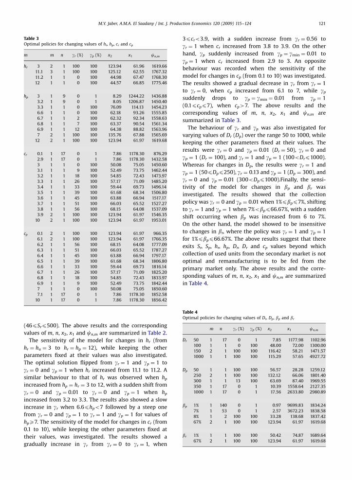
The sensitivity of the model for changes in hr (from

hr ¼ hu ¼ 3 to hr ¼ hp ¼ 12), while keeping the other

parameters fixed at their values was also investigated.

The optimal solution flipped from gr ¼ 1 and gp ¼ 1 to

gr ¼ 0 and gp ¼ 1 when hr increased from 11.1 to 11.2. A

similar behaviour to that of hr was observed when hp

increased from hp ¼ hr ¼ 3 to 12, with a sudden shift from

gr ¼ 0 and gp ¼ 0.01 to gr ¼ 0 and gp ¼ 1 when hp

increased from 3.2 to 3.3. The results also showed a slow

increase in gr when 6.6phpo7 followed by a steep one

from gr ¼ 0 and gp ¼ 1 to gr ¼ 1 and gp ¼ 1 for values of

hpX7. The sensitivity of the model for changes in cr (from

0.1 to 10), while keeping the other parameters fixed at

their values, was investigated. The results showed a

gradually increase in gr from gr ¼ 0 to gr ¼ 1, when

3pcro3.9, with a sudden increase from gr ¼ 0.56 to

gr ¼ 1 when cr increased from 3.8 to 3.9. On the other

hand, gp suddenly increased from gp ¼ gmin ¼ 0.01 to

gp ¼ 1 when cr increased from 2.9 to 3. An opposite

behaviour was recorded when the sensitivity of the

model for changes in cp (from 0.1 to 10) was investigated.

The results showed a gradual decrease in gr from gr ¼ 1

to gr ¼ 0, when cp increased from 6.1 to 7, while gp

suddenly drops to gp ¼ gmin ¼ 0.01 from gp ¼ 1

(0.1pcpp7), when cp47. The above results and the

corresponding values of m, n, x2, x1 and cn,m are

summarized in Table 3.

The behaviour of gr and gp was also investigated for

varying values of Dr (Dp) over the range 50 to 1000, while

keeping the other parameters fixed at their values. The

results were gr ¼ 0 and gp ¼ 0.01 (Dr ¼ 50), gr ¼ 0 and

gp ¼ 1 (Dr ¼ 100), and gr ¼ 1 and gp ¼ 1 (100oDrp1000).

Whereas for changes in Dp, the results were gr ¼ 1 and

gp ¼ 1 (50pDpp250), gr ¼ 0.13 and gp ¼ 1 (Dp ¼ 300), and

gr ¼ 0 and gp ¼ 0.01 (300oDpp1000).Finally, the sensi-

tivity of the model for changes in bp and br was

investigated. The results showed that the collection

policy was gr ¼ 0 and gp ¼ 0.01 when 1%pbpp7%, shifting

to gr ¼ 1 and gp ¼ 1 when 7%obpp66.67%, with a sudden

shift occurring when bp was increased from 6 to 7%.

On the other hand, the model showed to be insensitive

to changes in br, where the policy was gr ¼ 1 and gp ¼ 1

for 1%pbpp66.67%. The above results suggest that there

exits Sr, Sp, hr, hp, Dr, Dr and cp values beyond which

collection of used units from the secondary market is not

optimal and remanufacturing is to be fed from the

primary market only. The above results and the corre-

sponding values of m, n, x2, x1 and cn,m are summarized

in Table 4.

ARTICLE IN PRESS

M.Y. Jaber, A.M.A. El Saadany / Int. J. Production Economics 120 (2009) 115–124122

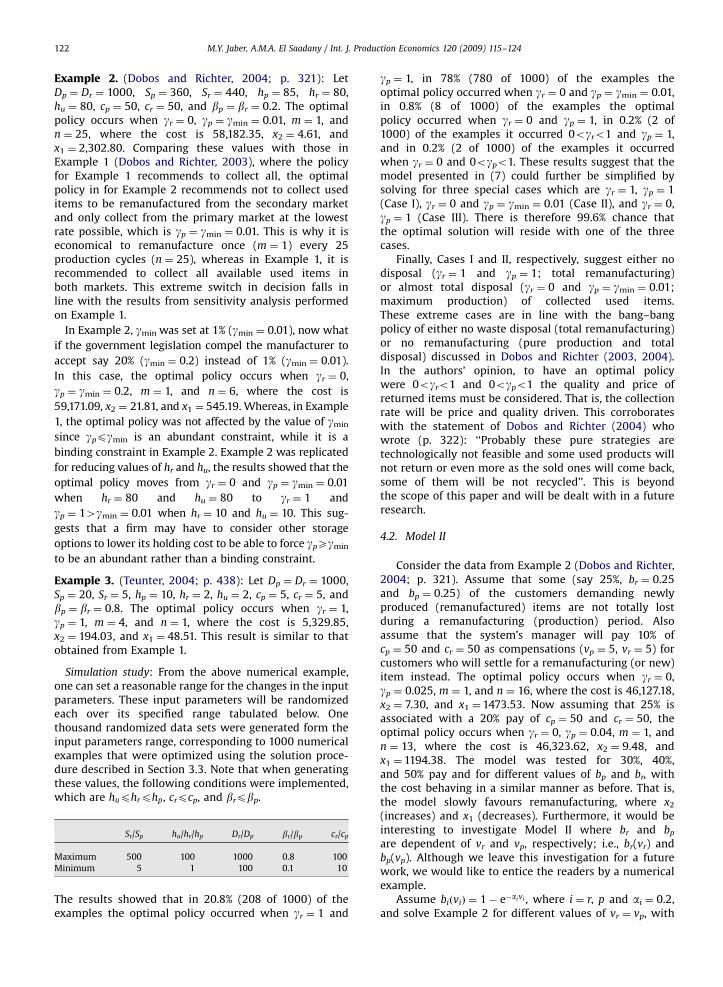
Example 2. (Dobos and Richter, 2004; p. 321): LetDp ¼ Dr ¼ 1000, Sp ¼ 360, Sr ¼ 440, hp ¼ 85, hr ¼ 80,hu ¼ 80, cp ¼ 50, cr ¼ 50, and bp ¼ br ¼ 0.2. The optimalpolicy occurs when gr ¼ 0, gp ¼ gmin ¼ 0.01, m ¼ 1, andn ¼ 25, where the cost is 58,182.35, x2 ¼ 4.61, andx1 ¼ 2,302.80. Comparing these values with those inExample 1 (Dobos and Richter, 2003), where the policyfor Example 1 recommends to collect all, the optimalpolicy in for Example 2 recommends not to collect useditems to be remanufactured from the secondary marketand only collect from the primary market at the lowestrate possible, which is gp ¼ gmin ¼ 0.01. This is why it iseconomical to remanufacture once (m ¼ 1) every 25production cycles (n ¼ 25), whereas in Example 1, it isrecommended to collect all available used items inboth markets. This extreme switch in decision falls inline with the results from sensitivity analysis performedon Example 1.

In Example 2, gmin was set at 1% (gmin ¼ 0.01), now what

if the government legislation compel the manufacturer to

accept say 20% (gmin ¼ 0.2) instead of 1% (gmin ¼ 0.01).

In this case, the optimal policy occurs when gr ¼ 0,

gp ¼ gmin ¼ 0.2, m ¼ 1, and n ¼ 6, where the cost is

59,171.09, x2 ¼ 21.81, and x1 ¼ 545.19. Whereas, in Example

1, the optimal policy was not affected by the value of gmin

since gppgmin is an abundant constraint, while it is a

binding constraint in Example 2. Example 2 was replicated

for reducing values of hr and hu, the results showed that the

optimal policy moves from gr ¼ 0 and gp ¼ gmin ¼ 0.01

when hr ¼ 80 and hu ¼ 80 to gr ¼ 1 and

gp ¼ 14gmin ¼ 0.01 when hr ¼ 10 and hu ¼ 10. This sug-

gests that a firm may have to consider other storage

options to lower its holding cost to be able to force gpXgmin

to be an abundant rather than a binding constraint.

Example 3. (Teunter, 2004; p. 438): Let Dp ¼ Dr ¼ 1000,Sp ¼ 20, Sr ¼ 5, hp ¼ 10, hr ¼ 2, hu ¼ 2, cp ¼ 5, cr ¼ 5, andbp ¼ br ¼ 0.8. The optimal policy occurs when gr ¼ 1,gp ¼ 1, m ¼ 4, and n ¼ 1, where the cost is 5,329.85,x2 ¼ 194.03, and x1 ¼ 48.51. This result is similar to thatobtained from Example 1.

Simulation study: From the above numerical example,one can set a reasonable range for the changes in the inputparameters. These input parameters will be randomizedeach over its specified range tabulated below. Onethousand randomized data sets were generated form theinput parameters range, corresponding to 1000 numericalexamples that were optimized using the solution proce-dure described in Section 3.3. Note that when generatingthese values, the following conditions were implemented,which are huphrphp, crpcp, and brpbp.

Sr/Sp

hu/hr/hp Dr/Dp br/bp cr/cp

Maximum

500 100 1000 0.8 100

Minimum

5 1 100 0.1 10

The results showed that in 20.8% (208 of 1000) of theexamples the optimal policy occurred when gr ¼ 1 and

gp ¼ 1, in 78% (780 of 1000) of the examples theoptimal policy occurred when gr ¼ 0 and gp ¼ gmin ¼ 0.01,in 0.8% (8 of 1000) of the examples the optimalpolicy occurred when gr ¼ 0 and gp ¼ 1, in 0.2% (2 of1000) of the examples it occurred 0ogro1 and gp ¼ 1,and in 0.2% (2 of 1000) of the examples it occurredwhen gr ¼ 0 and 0ogpo1. These results suggest that themodel presented in (7) could further be simplified bysolving for three special cases which are gr ¼ 1, gp ¼ 1(Case I), gr ¼ 0 and gp ¼ gmin ¼ 0.01 (Case II), and gr ¼ 0,gp ¼ 1 (Case III). There is therefore 99.6% chance thatthe optimal solution will reside with one of the threecases.

Finally, Cases I and II, respectively, suggest either nodisposal (gr ¼ 1 and gp ¼ 1; total remanufacturing)or almost total disposal (gr ¼ 0 and gp ¼ gmin ¼ 0.01;maximum production) of collected used items.These extreme cases are in line with the bang–bangpolicy of either no waste disposal (total remanufacturing)or no remanufacturing (pure production and totaldisposal) discussed in Dobos and Richter (2003, 2004).In the authors’ opinion, to have an optimal policywere 0ogro1 and 0ogpo1 the quality and price ofreturned items must be considered. That is, the collectionrate will be price and quality driven. This corroborateswith the statement of Dobos and Richter (2004) whowrote (p. 322): ‘‘Probably these pure strategies aretechnologically not feasible and some used products willnot return or even more as the sold ones will come back,some of them will be not recycled’’. This is beyondthe scope of this paper and will be dealt with in a futureresearch.

4.2. Model II

Consider the data from Example 2 (Dobos and Richter,2004; p. 321). Assume that some (say 25%, br ¼ 0.25and bp ¼ 0.25) of the customers demanding newlyproduced (remanufactured) items are not totally lostduring a remanufacturing (production) period. Alsoassume that the system’s manager will pay 10% ofcp ¼ 50 and cr ¼ 50 as compensations (vp ¼ 5, vr ¼ 5) forcustomers who will settle for a remanufacturing (or new)item instead. The optimal policy occurs when gr ¼ 0,gp ¼ 0.025, m ¼ 1, and n ¼ 16, where the cost is 46,127.18,x2 ¼ 7.30, and x1 ¼ 1473.53. Now assuming that 25% isassociated with a 20% pay of cp ¼ 50 and cr ¼ 50, theoptimal policy occurs when gr ¼ 0, gp ¼ 0.04, m ¼ 1, andn ¼ 13, where the cost is 46,323.62, x2 ¼ 9.48, andx1 ¼ 1194.38. The model was tested for 30%, 40%,and 50% pay and for different values of bp and br, withthe cost behaving in a similar manner as before. That is,the model slowly favours remanufacturing, where x2

(increases) and x1 (decreases). Furthermore, it would beinteresting to investigate Model II where br and bp

are dependent of vr and vp, respectively; i.e., br(vr) andbp(vp). Although we leave this investigation for a futurework, we would like to entice the readers by a numericalexample.

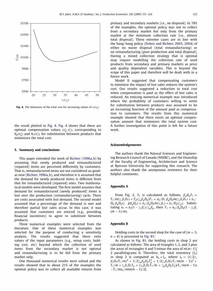
Assume biðviÞ ¼ 1� e�aivi , where i ¼ r, p and ai ¼ 0.2,and solve Example 2 for different values of vr ¼ vp, with

ARTICLE IN PRESS

9500

9700

9900

10100

10300

10500

10700

20

Cost

vr(vp)

25 30 35 40 45 50

Fig. 4. The behaviour of the total cost for increasing values of vr(vp).

M.Y. Jaber, A.M.A. El Saadany / Int. J. Production Economics 120 (2009) 115–124 123

the result plotted in Fig. 4. Fig. 4 shows that there areoptimal compensation values ðv�p; v

�r Þ, corresponding to

bpðv�pÞ and brðv�r Þ, for substitution between products thatminimizes the total cost.

5. Summary and conclusions

This paper extended the work of Richter (1996a, b) byassuming that newly produced and remanufactured(repaired) items are perceived differently by customers.That is, remanufactured items are not considered as-good-as new (Richter, 1996a, b), and therefore it is assumed thatthe demand for newly produced items is different fromthat for remanufactured (repaired) ones. Two mathema-tical models were developed. The first model assumes thatdemand for remanufactured (newly produced) items islost over the production (remanufacturing) cycle. Thereare costs associated with lost demand. The second modelassumed that a percentage of the demand is met andtherefore partial lost sales occur. In this case, it wasassumed that customers are enticed (e.g., providingfinancial incentives) to agree to substitute betweenproducts.

Three numerical examples were selected from theliterature. One of these numerical examples wasselected for the purpose of conducting a sensitivityanalysis. The results suggested that there exitsvalues of the input parameters (e.g., setup costs, hold-ing cost, etc) beyond which the collection of useditems from the secondary market is not optimaland remanufacturing is to be fed from the primarymarket only.

One thousand numerical results were solved and theresults showed that in about 21% of the examples theoptimal policy was to collect all available returns from

primary and secondary markets (i.e., no disposal). In 78%of the examples, the optimal policy was not to collectfrom a secondary market but only from the primarymarket at the minimum collection rate (i.e., almosttotal disposal). These extreme cases are in line withthe bang–bang policy (Dobos and Richter, 2003, 2004) ofeither no waste disposal (total remanufacturing) orno remanufacturing (pure production and total disposal).Having a mixed collection strategy that is optimalmay require modelling the collection rate of usedproducts from secondary and primary markets as priceand quality dependent variables. This is beyond thescope of this paper and therefore will be dealt with in afuture work.

Model II suggested that compensating customersto minimize the impact of lost sales reduces the system’scost. Our results suggested a reduction in total costwhen compensation is paid as the effect of lost sales isreduced. An enticing numerical example was introducedwhere the probability of customers willing to settlefor substitution between products was assumed to bean increasing function of the amount paid as compensa-tion to customers. The results from this numericalexample showed that there exists an optimal compen-sation amount that minimizes the total system cost.A further investigation of this point is left for a futurework.

Acknowledgements

The authors thank the Natural Sciences and Engineer-ing Research Council of Canada (NSERC), and the Deanshipof the Faculty of Engineering, Architecture and Scienceat Ryerson University for supporting this research. Theauthors also thank the anonymous reviewers for theirhelpful comments.

Appendix A

From Fig. 2, T1 is calculated as follows, bpDpT1 ¼

Tr=mðgrbrDrÞ þ TpðgpbpDpÞT1 ¼ x2=Dr :bpDpmðgrbrDrÞ þ x1=

Dp:bpDpðg pbpDpÞ ¼ x2=bpDpmðgrbrÞ þ x1=DpðgpÞ. Substi-tuting x1 ¼ x2ð1� grbrÞ=gpbp, then T1 ¼ x2=bpDpð1� grbr

ðm� 1Þ=mÞ.

Appendix B

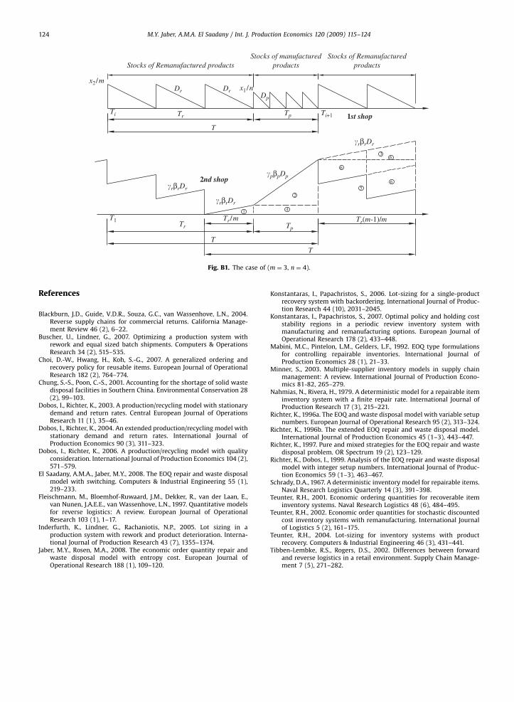
Holding costs in the second shop for the case of (m ¼ 3,n ¼ 4) is presented in Fig. B1:

As shown in Fig. B1, the holding costs in shop 2 arecalculated as follows: The area of triangles 1, 2, and 3 plusthe areas of rectangles 4 and 5 minus the area of m(m�1)/2 parallelograms 6. Therefore, the total inventory (Iu)in shop 2 is computed as hu� Iu, where Iu ¼ ½1=2gr

brDrðTr=mÞ2 þ 1=2gpbpDpT2p þ 1=2grbrDrðTr=mðm � 1ÞÞ2þ

Tr=mþ grbrDrTp þ ðgrbrDrTr=m þ gpbpDpTpÞðTr=mðm� 1ÞÞ�Tr=mx2=mmðm� 1Þ=2�.

ARTICLE IN PRESS

1st shop

2nd shop

Stocks of Remanufactured products

T

Stocks of manufacturedproducts

T1

Ti

x1/n

T

Ti+1

x2/mDr Dr

Dp

Tr Tp

T

Tr Tp

Tr/m1 4

2

65

3

Tr(m-1)/m

Stocks of Remanufacturedproducts

�rβrDr

�rβrDr

�rβrDr

�pβpDp

6

6

Fig. B1. The case of (m ¼ 3, n ¼ 4).

M.Y. Jaber, A.M.A. El Saadany / Int. J. Production Economics 120 (2009) 115–124124

References

Blackburn, J.D., Guide, V.D.R., Souza, G.C., van Wassenhove, L.N., 2004.Reverse supply chains for commercial returns. California Manage-ment Review 46 (2), 6–22.

Buscher, U., Lindner, G., 2007. Optimizing a production system withrework and equal sized batch shipments. Computers & OperationsResearch 34 (2), 515–535.

Choi, D.-W., Hwang, H., Koh, S.-G., 2007. A generalized ordering andrecovery policy for reusable items. European Journal of OperationalResearch 182 (2), 764–774.

Chung, S.-S., Poon, C.-S., 2001. Accounting for the shortage of solid wastedisposal facilities in Southern China. Environmental Conservation 28(2), 99–103.

Dobos, I., Richter, K., 2003. A production/recycling model with stationarydemand and return rates. Central European Journal of OperationsResearch 11 (1), 35–46.

Dobos, I., Richter, K., 2004. An extended production/recycling model withstationary demand and return rates. International Journal ofProduction Economics 90 (3), 311–323.

Dobos, I., Richter, K., 2006. A production/recycling model with qualityconsideration. International Journal of Production Economics 104 (2),571–579.

El Saadany, A.M.A., Jaber, M.Y., 2008. The EOQ repair and waste disposalmodel with switching. Computers & Industrial Engineering 55 (1),219–233.

Fleischmann, M., Bloemhof-Ruwaard, J.M., Dekker, R., van der Laan, E.,van Nunen, J.A.E.E., van Wassenhove, L.N., 1997. Quantitative modelsfor reverse logistics: A review. European Journal of OperationalResearch 103 (1), 1–17.

Inderfurth, K., Lindner, G., Rachaniotis, N.P., 2005. Lot sizing in aproduction system with rework and product deterioration. Interna-tional Journal of Production Research 43 (7), 1355–1374.

Jaber, M.Y., Rosen, M.A., 2008. The economic order quantity repair andwaste disposal model with entropy cost. European Journal ofOperational Research 188 (1), 109–120.

Konstantaras, I., Papachristos, S., 2006. Lot-sizing for a single-productrecovery system with backordering. International Journal of Produc-tion Research 44 (10), 2031–2045.

Konstantaras, I., Papachristos, S., 2007. Optimal policy and holding coststability regions in a periodic review inventory system withmanufacturing and remanufacturing options. European Journal ofOperational Research 178 (2), 433–448.

Mabini, M.C., Pintelon, L.M., Gelders, L.F., 1992. EOQ type formulationsfor controlling repairable inventories. International Journal ofProduction Economics 28 (1), 21–33.

Minner, S., 2003. Multiple-supplier inventory models in supply chainmanagement: A review. International Journal of Production Econo-mics 81-82, 265–279.

Nahmias, N., Rivera, H., 1979. A deterministic model for a repairable iteminventory system with a finite repair rate. International Journal ofProduction Research 17 (3), 215–221.

Richter, K., 1996a. The EOQ and waste disposal model with variable setupnumbers. European Journal of Operational Research 95 (2), 313–324.

Richter, K., 1996b. The extended EOQ repair and waste disposal model.International Journal of Production Economics 45 (1–3), 443–447.

Richter, K., 1997. Pure and mixed strategies for the EOQ repair and wastedisposal problem. OR Spectrum 19 (2), 123–129.

Richter, K., Dobos, I., 1999. Analysis of the EOQ repair and waste disposalmodel with integer setup numbers. International Journal of Produc-tion Economics 59 (1–3), 463–467.

Schrady, D.A., 1967. A deterministic inventory model for repairable items.Naval Research Logistics Quarterly 14 (3), 391–398.

Teunter, R.H., 2001. Economic ordering quantities for recoverable iteminventory systems. Naval Research Logistics 48 (6), 484–495.

Teunter, R.H., 2002. Economic order quantities for stochastic discountedcost inventory systems with remanufacturing. International Journalof Logistics 5 (2), 161–175.

Teunter, R.H., 2004. Lot-sizing for inventory systems with productrecovery. Computers & Industrial Engineering 46 (3), 431–441.

Tibben-Lembke, R.S., Rogers, D.S., 2002. Differences between forwardand reverse logistics in a retail environment. Supply Chain Manage-ment 7 (5), 271–282.