The Price of Inefficiency in Indian Agriculture

Flavius Badau

Economic Research Service, USDA

flavius.badau@ers.usda.gov

Nicholas E. Rada

Economic Research Service, USDA

nrada@ers.usda.gov

Selected Paper prepared for presentation at the Agricultural & Applied Economics

Association’s 2016 AAEA Meeting, Boston, MA, July 31 - Aug 2.

Copyright 2016 by Flavius Badau and Nicholas E. Rada. All rights reserved. Readers may make

verbatim copies of this document for non-commercial purposes by any means, provided this

copyright notice appears on all such copies.

All views expressed are those of the authors and not necessarily those of the Economic Research

Service or the U.S. Department of Agriculture.

1

1. Introduction/Motivation

Indian agriculture has, since the 1980s, increasingly shifted its output mix towards high value

commodities such as animal products and horticulture. The dominant share of this new-

commodity diversification occurred outside of North Indian, the epicenter of the country’s

intensive grain production model (Rada, 2016). India’s regional agricultural specialization is in

part due to national agricultural policies that are themselves highly regionalized and commodity-

specific, especially concerning output price supports, input subsidies, and commodity

procurement programs (Shreedhar, et al. 2012). For example, Minimum Support Prices – a

primary public policy lever to support remunerative prices for farmers – are applied to only

select commodities (predominately rice, wheat, and cotton) in a subset of producer states (NITI

Aayog, 2015).

India’s regional specialization may also be due to a misalignment of federal and state

agricultural policies. For example, in 2003 India’s national government passed the “Model Act”

to address market integration concerns stemming largely from the Essential Commodities Act

(ECA) and the Agricultural Product Marketing Committees (APMCs). As noted in World Bank

(2014), market reforms at the state-level have been only partially implemented; 12 of 18 states

have yet to fully adopt all key provisions of the Model Act. The combined effect of strong

national production priorities and imperfect policy adoption at the state level has led to

fragmented markets and distorted producer incentives. The World Bank (2014) suggests 68% of

potential short-run agricultural profits in India are lost to inefficiency, predominately from

farmers’ crop choice.

2

Our purpose is to predict farmer revenues if producers faced undistorted shadow prices and could

reallocate production to minimize technical inefficiency. To that end, we employ a newly

constructed 1980-2008 state-level production account of Indian agriculture, a distance frontier

specification, and an innovative output-reallocation predictive model to test whether India’s

farmers have achieved maximum potential revenues from their choice of crop mix given the

various policy, environmental, and input supply constraints.

2. Methodology

We model India’s agricultural technology, i.e. the tradeoff between agricultural commodities

produced, through an output set. Let P(x) denote this output set comprised of the vector of

outputsM

M Ryyy ),...,( 1 given by the inputs N

N Rxxx ),...,( 1 such that

yproducecanxyxP :)( . (1)

Standard properties stemming from an axiomatic framework include the free disposability of

inputs and outputs, and convexity and compactness of the output set P(x). Chambers et al.

(1996) discusses these properties in greater detail.

In order to examine the potential tradeoffs in producers’ output mix, a multi-output

representation of the technology is needed. We choose the directional output distance function

(DDF) because it offers a complete characterization of the output set as well as relative

performance measures. The DDF is defined as

)()(:max);,( xPgygyxD yyo

, (2)

with outputs expanded along a given directional vectorM

y Rg . In addition to representing the

agricultural production technology, the DDF also measures an observation’s distance to the best-

3

practice frontier, i.e. technical efficiency. If 0);,( yo gyxD

, that observation is located on the

frontier, the outer boundary of the output set, and is considered technically efficient. If

0);,( yo gyxD

, that observation is located inside the best-practice frontier and is considered

technically inefficient.

The DDF inherits its properties, i.e. Representation, Translation, Monotonicity, from the output

set.1 Representation says that the DDF completely characterizes the technology. The Translation

property is the additive analog of Shephard’s output distance function’s homogeneity property.

Monotonicity with respect to inputs is assumed to be non-negative, i.e. 0/);,( xgyxD yo

,

while monotonicity with respect to outputs is assumed to be non-positive, 0/);,( ygyxD yo

,

i.e. increasing outputs while holding inputs fixed decreases the value of the DDF, or decreases

the distance to the frontier (i.e. decreases inefficiency). Figure 1 illustrates the output set along

with the DDF, where point (y1, y2) is technically inefficient.

Fig. 1. Directional Output Distance Function

1 Please see Chambers et al. (1998) for greater detail of these properties.

P(x)

Y2

(y1+β*gy1, y2 β*gy2)

gy = (gy1, gy2)

(y1, y2)

Y1

4

From the DDF, parameter estimate β measures this observation’s distance to the frontier along

the direction vector, gy. In essence, it shows how much outputs would need to be scaled in order

for observation (y1, y2) to achieve technical efficiency.

2.1. Shadow pricing outputs

Assessing potential gains from improved efficiency requires two steps. The first step calculates

output shadow prices from the representative technology. The second step re-allocates outputs to

achieve technical efficiency. These new re-allocated values are then employed to predict

revenue. This section presents the first step while the next section presents the second step.

Exploiting the duality between the revenue function and the directional output distance function,

shadow prices for the output can be obtained provided that one of the output prices are known or

that observed total revenue stemming from the production of the outputs is known. In this study

we choose to employ the revenue approach following Fӓre, et al. (2015). Cross, et al. (2013)

have also employed this approach in the framework of an input requirement set exploiting the

duality between the cost function and the directional input distance function.

Following Fӓre et al. (2015), the duality between the revenue function and the directional output

distance function can be summarized as follows

0);,(:)(:),(11

yo

M

m

mmy

M

m

mmy

gyxDypmaxxPyypmaxpxR

(3)

In Lagrangian form, equation (3) becomes

yyoy

pggyxDpymaxpxR equaltoshownwaswhere));,((),(

.

Using ypg in the first order conditions (FOC) yields

5

),,( yoyy gyxDpgp

. (4)

Multiplying both sides by output vector y and using actual revenue (r) = py yields

ygyxD

rpg

yoy

y),,(

(5)

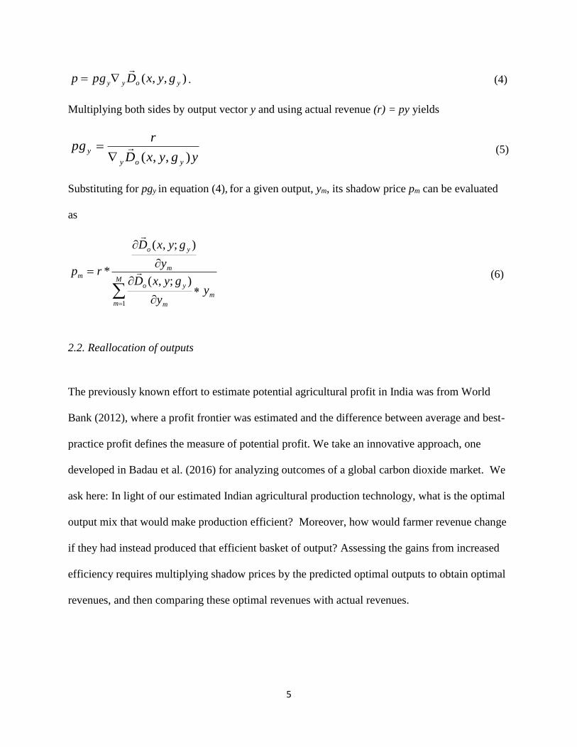
Substituting for pgy in equation (4), for a given output, ym, its shadow price pm can be evaluated

as

M

m

m

m

yo

m

yo

m

yy

gyxD

y

gyxD

rp

1

);,(

);,(

*

(6)

2.2. Reallocation of outputs

The previously known effort to estimate potential agricultural profit in India was from World

Bank (2012), where a profit frontier was estimated and the difference between average and best-

practice profit defines the measure of potential profit. We take an innovative approach, one

developed in Badau et al. (2016) for analyzing outcomes of a global carbon dioxide market. We

ask here: In light of our estimated Indian agricultural production technology, what is the optimal

output mix that would make production efficient? Moreover, how would farmer revenue change

if they had instead produced that efficient basket of output? Assessing the gains from increased

efficiency requires multiplying shadow prices by the predicted optimal outputs to obtain optimal

revenues, and then comparing these optimal revenues with actual revenues.

6

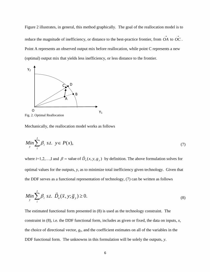
Figure 2 illustrates, in general, this method graphically. The goal of the reallocation model is to

reduce the magnitude of inefficiency, or distance to the best-practice frontier, from OA

to OC

.

Point A represents an observed output mix before reallocation, while point C represents a new

(optimal) output mix that yields less inefficiency, or less distance to the frontier.

Fig. 2. Optimal Reallocation

Mechanically, the reallocation model works as follows

. . ( ), I

iy

i

Min s t y P x (7)

where i=1,2,…,I and ),,(ofvalue yo gyxD

by definition. The above formulation solves for

optimal values for the outputs, y, as to minimize total inefficiency given technology. Given that

the DDF serves as a functional representation of technology, (7) can be written as follows

. . ( , ; ) 0.I

i o yy

i

Min s t D x y g (8)

The estimated functional form presented in (8) is used as the technology constraint. The

constraint in (8), i.e. the DDF functional form, includes as given or fixed, the data on inputs, x,

the choice of directional vector, gy, and the coefficient estimates on all of the variables in the

DDF functional form. The unknowns in this formulation will be solely the outputs, y.

B

D C

Y2

A

Y1 O

7

3. Estimation Strategy

We model India’s agriculture technology deterministically using a parametric directional output

distance function. Functional forms for directional distance functions have generally been

restricted to those functions that are linear in parameters which are referred to as the class of

transformed quadratic functions (Färe, et al. 2010). Färe and Lundberg (2005) solved for

functions that satisfy the directional distance function’s translation property and that are

simultaneously linear in parameters. They find as one of the two solutions the quadratic

function. The quadratic function has been suggested as a functional form that can accommodate

the translation property earlier by Chambers (1998).

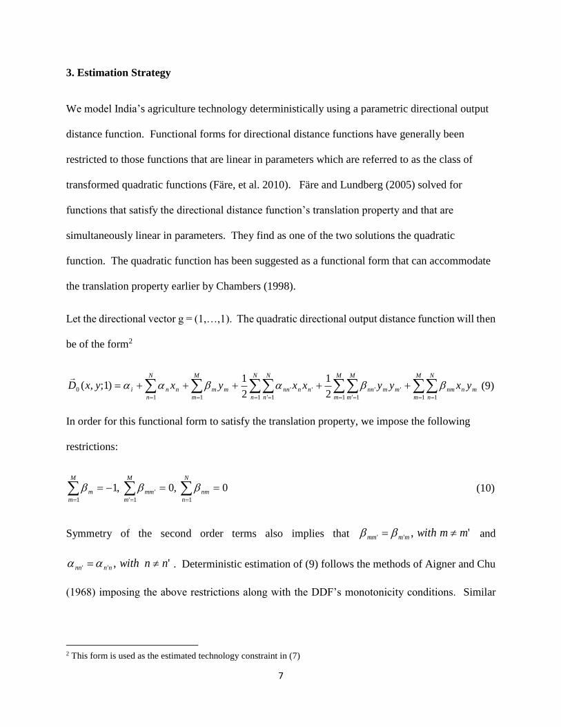
Let the directional vector g = (1,…,1). The quadratic directional output distance function will then

be of the form2

mn

M

m

N

n

nmmm

M

m

M

m

nnnn

N

n

N

n

nn

M

m

mmn

N

n

ni yxyyxxyxyxD

1 1

'

1 1'

''

1 1'

'

11

02

1

2

1)1;,(

(9)

In order for this functional form to satisfy the translation property, we impose the following

restrictions:

N

n

nm

M

m

mm

M

m

m

11'

'

1

0,0,1 (10)

Symmetry of the second order terms also implies that ','' mmwithmmmm and

','' nnwithnnnn . Deterministic estimation of (9) follows the methods of Aigner and Chu

(1968) imposing the above restrictions along with the DDF’s monotonicity conditions. Similar

2 This form is used as the estimated technology constraint in (7)

8

deterministic estimation of DDFs has been employed recently by Cross et al. (2013) and Bostian

and Herlihy (2014).

4. Data

In estimating our models, we make use of data on 63 outputs and 7 inputs, across 16 Indian states

and over the 1980-2008 period. The 63 outputs are aggregated into 6 output groups: grains,

pulses, horticulture, oilseeds, specialty products, and livestock products.3 We further control for

state-wise variations in rainfall and public agricultural research, as well as other state specific

unobservable, time-invariant heterogeneity. Bihar is grouped with Jharkhand to form Old Bihar,

Madhya Pradesh with Chhattisgarh to form Old Madhya Pradesh (Old MP), and Uttar Pradesh

with Uttaranchal to form Old Uttar Pradesh (Old UP) because these states split in year 2000. All

output and input data are measured in metric tons, and all prices are real (2004) prices, deflated

by the World Bank’s World Development Indicators GDP deflator specific to India. For our

present purposes, we have aggregated Old Madhya Pradesh, Assam, West Bengal, Old Bihar,

and Orissa into the C/E/NE region.

The 7 inputs include labor, land, materials, machinery capital, animal capital, energy, and time.

Labor reflects the total days worked per year in the agricultural sector by male and female

laborers. Net hectares of land are recorded annually and quality-differentiated into four groups:

irrigated cropland, rainfed cropland, pasture, and fallow land. Following Rada (2016), we

aggregate land into quality adjusted hectares of rainfed-equivalents using the following weights:

irrigated cropland (3.83), rainfed cropland (1.00), pasture (0.36), and fallow land (0.15).

Materials consist of total tonnage of N, P, and K applied by farms and specified in active

3 For more detail, please see Rada and Schimmelpfennig (2015).

9

ingredients. Machinery capital reflects the total stock of tractors, and animal capital the total

stock of animals on-farm. Energy is the total kilo-watt used by the agricultural sector, and time is

a general time trend which formally reflects the contribution of all unmeasured trending

variables.

Two control variables include state-wise rainfall variations and state agricultural research stocks.

The rainfall variable is specified as average annual means in millimeters. The agricultural

research stock includes state agricultural university (SAU) as well as ICAR research

expenditures, and follows the trapezoidal structure estimated in Rada and Schimmelpfennig

(2015). To control for state specific unobservable characteristics we also include indicator

variables for every Indian state.

5. Estimation Results

In predicting India’s optimal agricultural revenues, we first determine the level of technical

inefficiency present over the 1980-2008 period. We then estimate shadow prices and predict

optimal output allocations and revenues. To conserve space, the 158 estimated parameters of the

quadratic DDF are not presented here but are available upon request. All estimations (the DDF

and the reallocation model) took place using the software GAMS.

5.1 Shadow Prices

Over the entire study period we find that, on average at the national level, in order to be efficient,

i.e. produce on the frontier of the output set, the average observation needed to add 0.186 to each

of the 6 outputs (Y1+0.186, Y2+0.186,…). In other words, we find 18.6% technical inefficiency

in India’s agricultural production over the 1980-2008 time period.

10

Given DDF parameter estimates, data on the inputs and the outputs, and data on actual observed

revenues, we calculate output shadow prices based on equation (6). Recalling equation (6),

shadow prices are calculated using actual observed real revenue, adjusting for each output’s

impact on technology (.) / 0o mD y and normalized by the combined outputs’ impact on

technology.

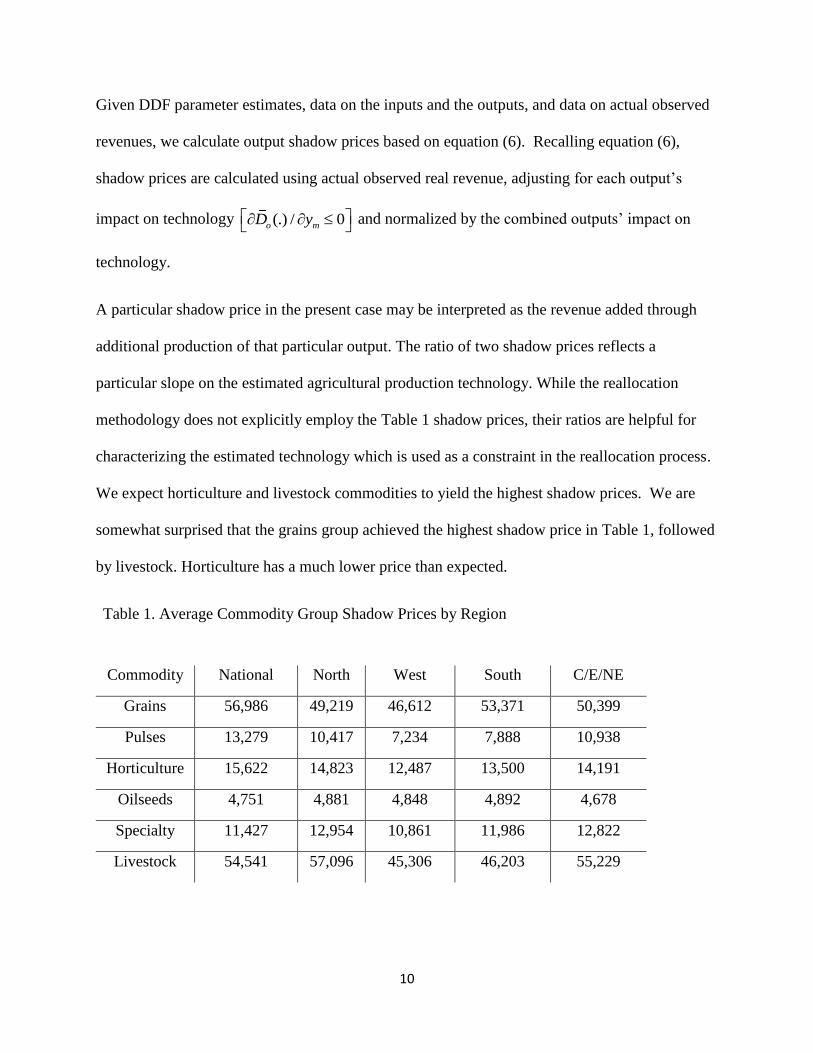
A particular shadow price in the present case may be interpreted as the revenue added through

additional production of that particular output. The ratio of two shadow prices reflects a

particular slope on the estimated agricultural production technology. While the reallocation

methodology does not explicitly employ the Table 1 shadow prices, their ratios are helpful for

characterizing the estimated technology which is used as a constraint in the reallocation process.

We expect horticulture and livestock commodities to yield the highest shadow prices. We are

somewhat surprised that the grains group achieved the highest shadow price in Table 1, followed

by livestock. Horticulture has a much lower price than expected.

Table 1. Average Commodity Group Shadow Prices by Region

Commodity National North West South C/E/NE

Grains 56,986 49,219 46,612 53,371 50,399

Pulses 13,279 10,417 7,234 7,888 10,938

Horticulture 15,622 14,823 12,487 13,500 14,191

Oilseeds 4,751 4,881 4,848 4,892 4,678

Specialty 11,427 12,954 10,861 11,986 12,822

Livestock 54,541 57,096 45,306 46,203 55,229

11

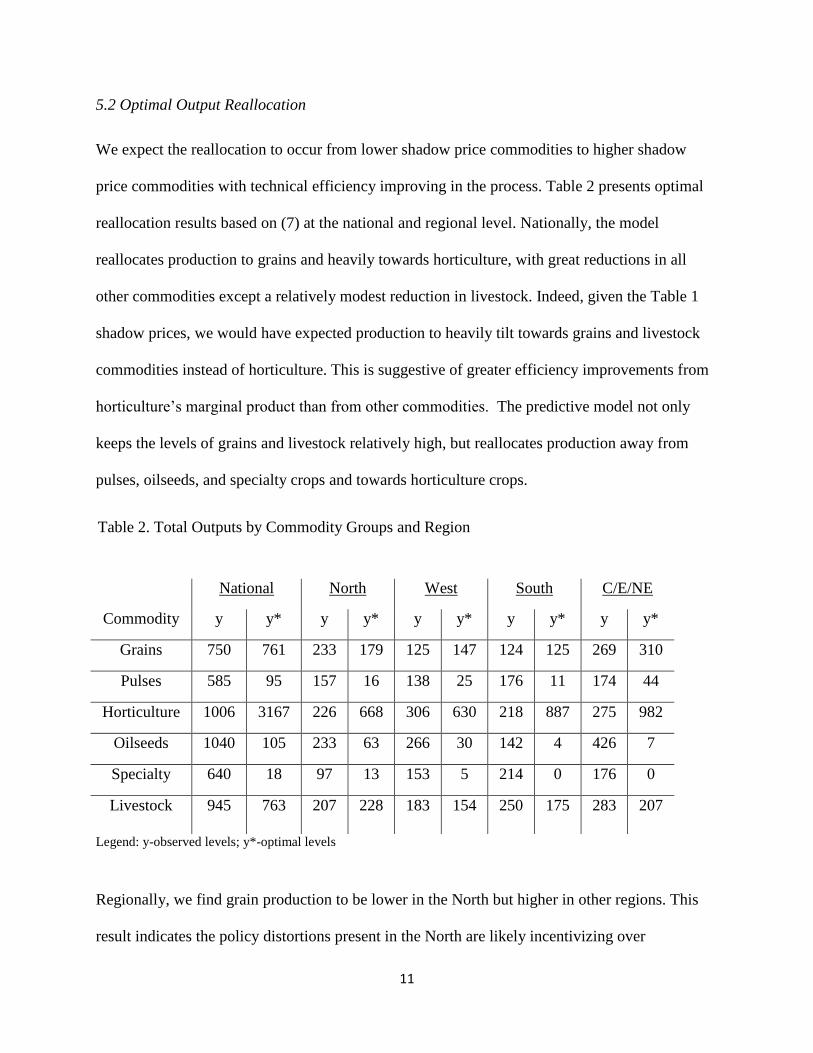
5.2 Optimal Output Reallocation

We expect the reallocation to occur from lower shadow price commodities to higher shadow

price commodities with technical efficiency improving in the process. Table 2 presents optimal

reallocation results based on (7) at the national and regional level. Nationally, the model

reallocates production to grains and heavily towards horticulture, with great reductions in all

other commodities except a relatively modest reduction in livestock. Indeed, given the Table 1

shadow prices, we would have expected production to heavily tilt towards grains and livestock

commodities instead of horticulture. This is suggestive of greater efficiency improvements from

horticulture’s marginal product than from other commodities. The predictive model not only

keeps the levels of grains and livestock relatively high, but reallocates production away from

pulses, oilseeds, and specialty crops and towards horticulture crops.

Table 2. Total Outputs by Commodity Groups and Region

National North West South C/E/NE

Commodity y y* y y* y y* y y* y y*

Grains 750 761 233 179 125 147 124 125 269 310

Pulses 585 95 157 16 138 25 176 11 174 44

Horticulture 1006 3167 226 668 306 630 218 887 275 982

Oilseeds 1040 105 233 63 266 30 142 4 426 7

Specialty 640 18 97 13 153 5 214 0 176 0

Livestock 945 763 207 228 183 154 250 175 283 207

Legend: y-observed levels; y*-optimal levels

Regionally, we find grain production to be lower in the North but higher in other regions. This

result indicates the policy distortions present in the North are likely incentivizing over

12

production of grains, which is consistent with evidence that northern India’s intensive grain

production have suffered significant natural resource degradation (Murgai et al., 2001) and

excessive groundwater exploitation (Akermann, 2012). The model predicts that to minimize

inefficiency the North would move towards commodities of higher value, such as horticulture

and to a lesser extent towards animal products such as milk. But the North is not unique, all

regions would need to substantial increase horticulture production. Livestock production, on the

other hand, would decline in all regions apart from the North.

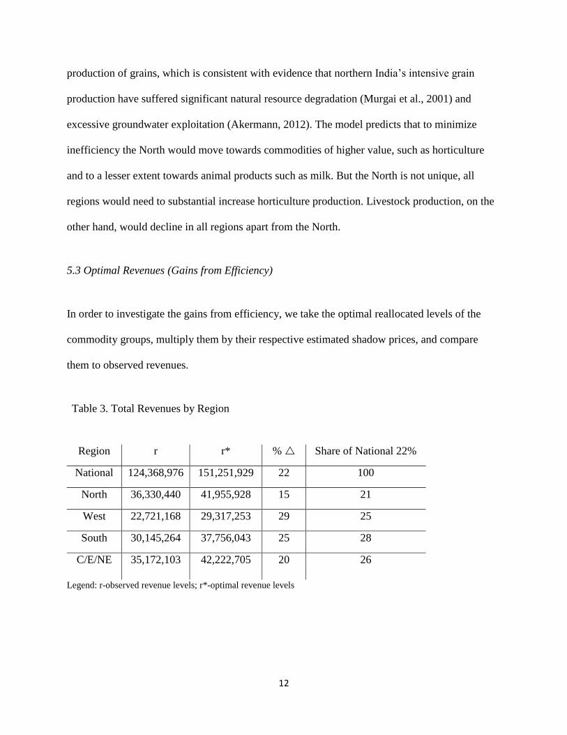
5.3 Optimal Revenues (Gains from Efficiency)

In order to investigate the gains from efficiency, we take the optimal reallocated levels of the

commodity groups, multiply them by their respective estimated shadow prices, and compare

them to observed revenues.

Table 3. Total Revenues by Region

Region r r* % Share of National 22%

National 124,368,976 151,251,929 22 100

North 36,330,440 41,955,928 15 21

West 22,721,168 29,317,253 29 25

South 30,145,264 37,756,043 25 28

C/E/NE 35,172,103 42,222,705 20 26

Legend: r-observed revenue levels; r*-optimal revenue levels

13

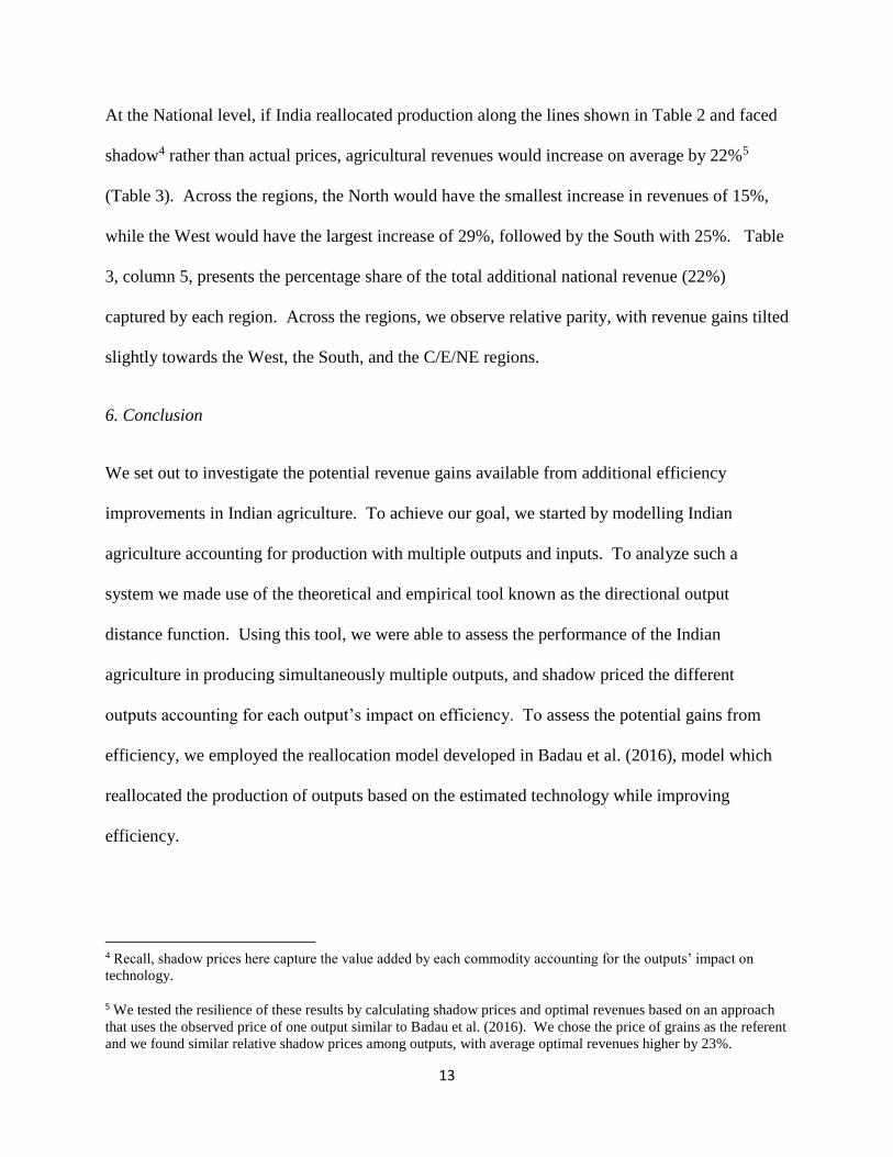
At the National level, if India reallocated production along the lines shown in Table 2 and faced

shadow4 rather than actual prices, agricultural revenues would increase on average by 22%5

(Table 3). Across the regions, the North would have the smallest increase in revenues of 15%,

while the West would have the largest increase of 29%, followed by the South with 25%. Table

3, column 5, presents the percentage share of the total additional national revenue (22%)

captured by each region. Across the regions, we observe relative parity, with revenue gains tilted

slightly towards the West, the South, and the C/E/NE regions.

6. Conclusion

We set out to investigate the potential revenue gains available from additional efficiency

improvements in Indian agriculture. To achieve our goal, we started by modelling Indian

agriculture accounting for production with multiple outputs and inputs. To analyze such a

system we made use of the theoretical and empirical tool known as the directional output

distance function. Using this tool, we were able to assess the performance of the Indian

agriculture in producing simultaneously multiple outputs, and shadow priced the different

outputs accounting for each output’s impact on efficiency. To assess the potential gains from

efficiency, we employed the reallocation model developed in Badau et al. (2016), model which

reallocated the production of outputs based on the estimated technology while improving

efficiency.

4 Recall, shadow prices here capture the value added by each commodity accounting for the outputs’ impact on

technology.

5 We tested the resilience of these results by calculating shadow prices and optimal revenues based on an approach

that uses the observed price of one output similar to Badau et al. (2016). We chose the price of grains as the referent

and we found similar relative shadow prices among outputs, with average optimal revenues higher by 23%.

14

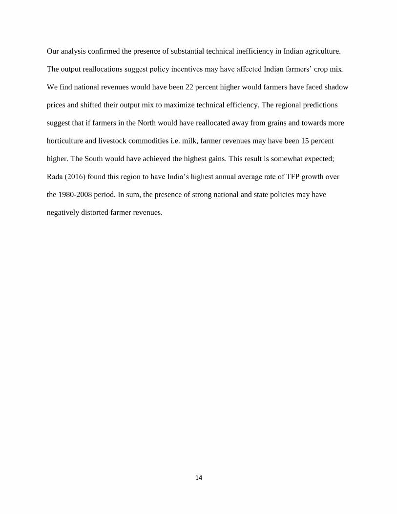
Our analysis confirmed the presence of substantial technical inefficiency in Indian agriculture.

The output reallocations suggest policy incentives may have affected Indian farmers’ crop mix.

We find national revenues would have been 22 percent higher would farmers have faced shadow

prices and shifted their output mix to maximize technical efficiency. The regional predictions

suggest that if farmers in the North would have reallocated away from grains and towards more

horticulture and livestock commodities i.e. milk, farmer revenues may have been 15 percent

higher. The South would have achieved the highest gains. This result is somewhat expected;

Rada (2016) found this region to have India’s highest annual average rate of TFP growth over

the 1980-2008 period. In sum, the presence of strong national and state policies may have

negatively distorted farmer revenues.

15

References

1. Akermann, R. 2012. New directions for water management in Indian agriculture. Global

Journal of Emerging Market Economies 4(2):227-288.

2. Badau, F., Fӓre, R., M. Gopinath (2016). Global resilience to climate change: Examining

global economic and environmental performance resulting from a global carbon dioxide

market. Resource and Energy Economics, forthcoming.

3. Bostian, M., Herlihy, A. (2014). Valuing tradeoffs between agricultural production and

wetland condition in the U.S. Mid-Atlantic region. Ecological Economics, 105, 284-291.

4. Chambers, R. (1998). Input and output indicators. In: Färe, R., Grosskopf, S., Russell,

R.R. (Eds.), Index Numbers in Honour of Sten Malmquist (pp. 241-272). Boston: Kluwer

Academic Publishers.

5. Chambers, R., Chung, Y., Färe, R. (1998). Profit, directional distance functions, and

Nerlovian efficiency. Journal of Optimization Theory and Applications, 98, 351–364.

6. Cross, R., Fӓre, R., Grosskopf, S., Weber, W. (2013). Valuing Vineyards: A Directional

Distance Function Approach. Journal of Wine Economics, 8 (1), 69-82.

7. Färe, R., Grosskopf, S., Margaritis, D. (2015). Pricing Nonmarketed Goods using

Distance Functions. Mimeo. Oregon State University and University of Auckland.

8. Färe, R., Lundberg, A. (2005). Parameterizing the Shortage (Directional Distance)

Function. Oregon State University Working Paper.

9. Färe, R., Martins-Filho, C., and Vardanyan, M. (2010). On Functional Form

Representation of Multi-Output Production Technologies. Journal of Productivity

Analysis, 33, 81-96.

16

10. Murgai, R., Ali, M., and Byerlee, D., 2001. Productivity growth and sustainability in

post-green revolution agriculture: The case of the Indian and Pakistan Punjabs. World

Bank Res. Obs. 16 (2), 199–218.

11. NITI Aayog (2015). Raising Agricultural Productivity and Making Farming

Remunerative for Farmers. An Occasional Paper, National Institution for Transforming

India (NITI) Aayog, Government of India, December 2015.

12. Rada, N., and Schimmelpfennig, D. (2015). Propellers of Agricultural Productivity

Growth in India. ERR-203, Economic Research Service, U.S. Department of Agriculture.

Available at: http://www.ers.usda.gov/publications/err-economic-research-

report/err203.aspx

13. Rada, N. (2016). India’s Post-Green-Revolution Agricultural Performance: What is

Driving Growth? Agricultural Economics, 47 (3). Available at:

http://onlinelibrary.wiley.com/doi/10.1111/agec.12234/abstract

14. Shreedhar, G., N. Gupta, H. Pullabhotla, A. Ganesh-Kumar, and A. Gulati, 2012. A

Review of Input and Output Policies for Cereals Production in India. International Food

Policy Research Institute (IFPRI) Discussion Paper 01159. New Delhi, India.

15. World Bank (2014). Republic of India: Accelerating Agricultural Productivity Growth.

World Bank Report No. 88093-IN, May, 2014, Washington, DC. Available at:

https://openknowledge.worldbank.org/handle/10986/18736

17